Curvature-driven instabilities in thin active shells

Elastic structures under load are often susceptible to dramatic instabilities such as the buckling of a column under compression[1, 2], or the collapse of a vessel under pressure [3, 4]. Traditionally, engineers have studied instabilities to avoid them as they lead to softening, fracture and failure. However, recently, the study of instabilities has been revitalised by the growing interest in soft materials such as gels, elastomers and biological tissues. Soft materials can undergo large strains without failing, meaning they survive instabilities and are thus capable of dramatic shape changes [5]. Furthermore, many soft materials can undergo active strain deformations, including swelling gels [6, 7, 8, 9, 10], growth in biological tissues [11, 12, 13, 14], uniaxial contraction in liquid crystal elastomerss [15, 16, 17, 18] and biological muscles, and inflation in barromorphs [19, 20] and other pneumatic systems[21]. When these active strain are homogeneous across the material, one obtains simple shape changes. However, when they are inhomogeneous, they are also often geometrically incompatible, meaning that there is no corresponding displacement field that allows the system to fully relax, leading to internal stresses even in the energy minimising state.

Such incompatible spontaneous deformations can trigger spontaneous elastic instabilities, in which the system suddenly adopts a new and more complex shape. For example, a growing layer on a soft substrate can wrinkle due to the inter-facial mismatch between the length of the layer and the substrate it is attached to[22, 23, 24, 25, 26]. Biology uses such growth-induced wrinkling to form brain folds [27, 28], villi [29], and gut loops [30]. In thin shell-like structures, incompatible active deformations generate instabilities such as the snap of a Venus fly-trap [31], the folding of a pollen grain [32, 33, 34] and the bistability of a cyclists snap-band [35]. These different shell instabilities have been addressed individually, but a clear and intuitive overview of their behaviour is still lacking. Here, we make a start by presenting a complete and simple treatment of incompatibility driven instabilities and states in thin and shallow shells, highlighting the different behaviours of positive, zero and negative Gauss curvature geometries.

Due to their slenderness, thin shells can be represented by a 2D surface. Any surface in 3D euclidean space can be described by its intrinsic and extrinsic properties. The intrinsic geometry is characterised by distances between points on the surface, captured by the metric tensor ${{\bm{a}}}$. The extrinsic geometry is locally described by the two principal curvatures $\kappa_{1}$ and $\kappa_{2}$, identified by inscribing the largest and smallest possible circles tangent to the surface, as shown in Fig. 1a). Mathematically, aligning the coordinate system with the curvature directions, means the curvature is described by the tensor ${{\bm{\kappa}}}=\text{diag}(\kappa_{1},\kappa_{2})$. However, crucially, ${{\bm{a}}}$ and ${{\bm{\kappa}}}$ cannot be chosen independently — in any real surface, they must satisfy geometric compatibility conditions. Most famously, they must satisfy Gauss’s theorema egregium,stating that the Gauss curvature $K=\det{{{\bm{\kappa}}}}=\kappa_{1}\kappa_{2}$ is an intrinsic property of the surface and can be computed directly from the metric [36].

In physical shells, active shape changes can separately modify the locally preferred metric $\bar{{{\bm{a}}}}$ by changing in-plane distances [7, 9, 10, 15, 16, 17, 18, 19, 37, 38], and the locally preferred curvature $\bar{{{\bm{\kappa}}}}$ via in-thickness variations, reminiscent of the bending of a bi-metal strip [39, 37]. However, given they are controlled by independent mechanisms, it is possible for $\bar{{{\bm{\kappa}}}}$ and $\bar{{{\bm{a}}}}$ to not satisfy the compatibility conditions, meaning that there is no surface that achieves all the preferred characteristics. Such incompatibility between $\bar{{{\bm{\kappa}}}}$ and $\bar{{{\bm{a}}}}$ is the appropriate dimensionally reduced version of general geometric incompatibility in bulk elasticity [40] and results in the physical shell always being internally stressed, even in their energy minimizing state. These internal stresses in turn underpin the instabilities observed in active shells. A key aspect of the mechanics of thin shells is that deforming the metric from $\bar{{{\bm{a}}}}$ requires stretching, with an energetic penalty proportional to thickness $t$, while deforming the extrinsic curvature from $\bar{{{\bm{\kappa}}}}$ only incurs a much smaller bending energy cost proportional to $t^{3}$. Thus in thin shells, isometric bending deformations are favoured wherever possible.

A simple example of incompatibility and instability arises in a spherical bi-layer gel cap. If we assume the cap was prepared by casting directly in the spherical state, it will have two equal principal curvatures, $1/R$, and homogeneous positive Gauss curvature $K=1/R^{2}$. These curvatures will also be the preferred values, meaning the cap is compatible and unstressed. The hallmark of this compatibility is that, if we dissect a thin strip from the cap, it will not relax in shape, but retain the same curvature it had whilst part of the cap. However, if we now imagine the upper layer swells mildly (or thermally expands) relative to the lower layer, this will increase the preferred extrinsic curvature beyond $1/R$ whilst having a negligible effect on the metric. Unfortunately, the shell cannot adopt this increased curvature without also increasing the Gauss curvature, which would require an energetically prohibitive stretch. Instead, it will remain in the same shape, but now with internal stresses; if we now dissect out a thin strip, it will be released from its metric constraints and relax to its preferred curvature, as illustrated in Fig. 1b). In this case, further swelling of the top layer ultimately triggers an instability in which the spherical cap looses rotational symmetry and ultimately folds [41], as shown in Fig. 1b). Conversely, large swelling of the bottom layer promotes bends with opposite sign to the original state, as shown in Fig. 1c). These will eventually drive the snap inversion of the cap, reminiscent of the inversion of a bimetallic dome used in kettle switches, and the snap of a rubber-popper toy [42]. Thus, even in this simple case, we may see two different instabilities, driven by different senses of incompatibility between extrinsic and intrinsic preferred curvature.

Importantly, different instabilities involve different mechanics, as some may proceed purely isometrically, while others require stretching. This difference is reflected in the thickness dependence of the buckling threshold. For example, the folding of the spherical cap subject to a curvature load proceeds via isometries, so the stretching energy is zero, and the threshold is thus thickness independent, requiring only a mild excess curvature $\delta\bar{\kappa}=\kappa-\bar{\kappa}\sim 1/R$. Conversely, the inside-out snapping of the cap inevitably requires stretching and is thus non-isometric. In reality, this instability nucleates at the boundary of the system where bend and stretch compete in a layer of width $\sim 1/\sqrt{Rt}$, leading to a much higher buckling threshold that scales like $\delta\bar{\kappa}\sim 1/\sqrt{Rt}$ [41]. Finally, a fully closed spherical shells has no isometries available and there is no boundary, leading to a yet-higher buckling threshold scaling like $\delta\bar{\kappa}\sim 1/t$ [41].

By combining casting with initial preferred curvature, gel-like swelling spontaneous shape changes, and nematic-elastomer/muscle-like uniaxial spontaneous shape changes, a shell may undergo almost arbitrary programmed changes to ${{\bm{\bar{a}}}}$ and ${{\bm{\bar{\kappa}}}}$ [16, 17, 18, 37]. In this article, we offer a simple and comprehensive treatment of curvature driven instabilities in thin, shallow shells with arbitrary but homogeneous preferred curvatures. In such very-thin shells, the different scaling of stretching and bending means that the stretching energy turns into a constraint on the metric and hence the Gauss curvature, so one only has instabilities that proceed isometrically, with mild threshold curvature loads $\delta\bar{\kappa}\sim\sqrt{K}$. Nevertheless, despite this limitation, the model includes a wide variety of instabilities, in which the principle curvatures of the shell break-symmetry, rotate and invert. The first type of instability is associated with supercritical spontaneous symmetry breaking and comes in two flavours: the continuous symmetry breaking of isotropy, and discrete breaking of up/down symmetry. The rotation instability is a 90 degree rotation between states of broken isotropy which occurs via a Goldstone-like mode, characterised by a change in configuration but not in energy. Conversely, the inversion instability occur as a subcritical jump between states of broken up/down symmetry and are associated with bi-stability.

We summarise these results by plotting phase diagrams for active shells with zero, positive and negative Gauss curvature, which show how the state of the shell changes with preferred curvature, and where the different instabilities arise. Importantly, our model uncovers new instabilities, especially in the previously little discussed negative Gauss curvature systems. It also offers a much simpler perspective on several known instabilities which had previously been understood using more-complicated boundary layer physics and/or ad-hoc assumptions. Finally, although our model is for shallow shells, in the final section, we show that the threshold it predicts for the folding of a shallow spherical cap also extends to deep spherical caps.

Our task is to find the achieved shape of a shallow and thin shell with a homogeneous preferred curvature $\bar{{{\bm{\kappa}}}}$, and also a preferred metric $\bar{{{\bm{a}}}}$ that, via the theoroma egregium, encodes a homogeneous Gauss curvature $K$. Since the shell is thin, we may assume it adopts a final form that exactly achieves $\bar{{{\bm{a}}}}$, and hence bears no stretch energy. Furthermore, since the shell is shallow, the achieved surface is approximated by a quadratic form $r(x,y)=(x,y,{\textstyle\frac{1}{2}}\kappa_{1}x^{2}+{\textstyle\frac{1}{2}}\kappa_{2}y^{2}),$ where $\kappa_{1}$ and $\kappa_{2}$ are the achieved principal curvatures, and $(x,y)$ are Cartesian coordinates in a tangent plane at the origin, aligned with the curvature tensor ${{\bm{\kappa}}}=\text{diag}(\kappa_{1},\kappa_{2})$. If the preferred curvature is ${{\bm{\bar{\kappa}}}}$, then the bending energy of the shell will be [40]:

$$\mathcal{E}_{b}=\frac{Et^{3}}{24(1+\nu^{2})}\int\left[(1-\nu){\text{Tr}{({{\bm{\kappa}}}-\bar{{{\bm{\kappa}}}})}}^{2}+\nu\left({\text{Tr}{({{\bm{\kappa}}}-\bar{{{\bm{\kappa}}}})}}\right)^{2}\right]\,dA.$$

(1)

Since the shell bears no stretch energy, the curvature, and thus shape achieved by the shell, corresponds to a minimum of this bend energy. However, the minimisation is constrained by the theorema egregium, which dictates that the Gauss curvature $\kappa_{1}\kappa_{2}$ of the surface is an intrinsic property of the metric, and hence must match $K$ as encoded by ${{\bm{\bar{a}}}}$, giving a compatibility constraint between curvature and metric:

$$K=\det{{{\bm{\kappa}}}}=\kappa_{1}\kappa_{2}.$$

(2)

Formally, there are two further compatibility equations, known as the Codazzi-Mainardi equations, which also feature the metric connection computed from ${{\bm{\bar{a}}}}$. However, the Cartesian coordinate system ($x,y$) forms a normal coordinate system for ${{\bm{\bar{a}}}}$, meaning it is not only orthonormal, but all the connections vanish at the origin, so the Codazzi-Mainardi are automatically satisfied near the origin (and hence throughout our shallow shell) provided ${{\bm{\kappa}}}$ too is homogeneous, as it is in our quadratic surface. Furthermore, since both ${{\bm{\kappa}}}$ and $\bar{{{\bm{\kappa}}}}$ are homogeneous, we can trivially evaluate the integral in 1 to get

$$\mathcal{E}_{b}=\frac{AEt^{3}}{24(1+\nu^{2})}\left[(1-\nu){\text{Tr}{({{\bm{\kappa}}}-\bar{{{\bm{\kappa}}}})}}^{2}+\nu\left({\text{Tr}{({{\bm{\kappa}}}-\bar{{{\bm{\kappa}}}})}}\right)^{2}\right]$$

(3)

where $A$ is the area of the shell. Therefore, our task is simply to minimise Eq. 3 over ${{\bm{\kappa}}}$, subject to Eq. 2. Before we proceed, it is convenient to further simplify the problem by introducing

$$H={\textstyle\frac{1}{2}}{\text{Tr}{({{\bm{\kappa}}})}}={\textstyle\frac{1}{2}}(\kappa_{1}+\kappa_{2})\,\,\,\,\,\,\,\,\text{and}\,\,\,\,\,\,\,\,\,D={\textstyle\frac{1}{2}}(\kappa_{1}-\kappa_{2}),$$

which represent the mean achieved curvature and mean difference in achieved curvature of the shell, and the corresponding quantities $\bar{H}={\textstyle\frac{1}{2}}(\bar{\kappa}_{1}+\bar{\kappa}_{2})$ and $\bar{D}={\textstyle\frac{1}{2}}(\bar{\kappa}_{1}-\bar{\kappa}_{2})$ for the preferred curvature. Substituting these into eqn. 3 and re-scaling to eliminate the prefactor, we see the problem is equivalent to minimising

$$\tilde{\mathcal{E}_{b}}=(H-\bar{H})^{2}+\gamma(D-\bar{D})^{2}+4D\bar{D}\sin^{2}\theta,$$

(4)

where $\theta$ is the angle between the principal directions of ${{\bm{\kappa}}}$ and $\bar{{{\bm{\kappa}}}}$, and $\gamma=(1+\nu)/(1-\nu)\geq 1$ captures Poisson effects. Minimisation over ${{\bm{\kappa}}}$ is now represented by minimisation over $H$, $D$ and $\theta$, while $\bar{D}$ and $\bar{H}$, (preferred curvature) are held constant. Minimisation is subject to the reformulated Gauss constraint:

$$K=H^{2}-D^{2}.$$

(5)

Before minimising the energy, we clarify two subtleties in the new parameterization. First, a rotation of the achieved curvature by $\theta=\pi/2$ is equivalent to inverting the roles of $\kappa_{1}$ and $\kappa_{2}$, which is also achieved by sending $D\to-D$ without changing $H$ and $\theta$. Although this might appear as a redundancy, it is helpful to maintain both $D$ and $\theta$ when studying the stability of an equilibrium. Secondly, flipping the signs of $D$, $\bar{D}$, $H$ and $\bar{H}$ leaves the energy unchanged. This is a consequence of the arbitrary definition of positive vs negative curvature. Thus, when studying instabilities, we can often concentrate on a restricted set of values of $\bar{D}$ and $\bar{H}$, then use these facts to extend our theory to all values of the preferred bend.

In the remainder of this section, we shall discuss this minimisation explicitly for the cases when $K=0$, $K>0$ and $K<0$. In each case, we shall present a 2D phase diagram, showing the achieved states of the shell as a function of $\bar{H}$ and $\bar{D}$. Active changes in the shell are then represented by changes in the preferred curvatures, $\bar{H}$ and $\bar{D}$, causing the shell to trace out a path on the phase diagram, and instabilities occur when this line passes from one region to another, indicating a qualitative change in the shape of the shell.

As discussed in section 33.23.2.1, a shallow spherical cap subject to an excess preferred curvature looses rotational symmetry and folds when the preferred curvature exceeds a critical value $\bar{\kappa}_{c}=\frac{2}{1+\nu}\sqrt{K}$, promoting the folding of the structure. In this section, we show that critical buckling load and the 2-fold symmetric buckled shape predicted by the simple shallow model are correct even in deep shells, highlighting the shallow model’s value.

We start by considering a spherical shell with angular depth $\theta_{0}$, and described with spherical coordinates $(R,\theta,\phi)$ as shown in Fig. 5a). We take an isotropic preferred curvature ${{\bm{\bar{\kappa}}}}=\bar{\kappa}{{\bm{I}}}$, as would result in a bilayer gel shell, and, without loss of generality, we set $K=1$. Following our work for the shallow shell, let us write the principal curvatures as:

	$\displaystyle\kappa_{1}(\theta,\phi)$	$\displaystyle=H(\theta,\phi)+D(\theta,\phi)$		(28)
	$\displaystyle\kappa_{2}(\theta,\phi)$	$\displaystyle=H(\theta,\phi)-D(\theta,\phi)$		(29)

where $H={\textstyle\frac{1}{2}}(\kappa_{1}+\kappa_{2})>0$ is the mean curvature and $D={\textstyle\frac{1}{2}}(\kappa_{1}-\kappa_{2})$ is the curvature asymmetry. Note that $H$ and $D$ now depend on the position of the shell via $\theta$ and $\phi$. However, for sake of conciseness, we will avoid writing explicitly the dependence. The Gauss constraint requires:

$$K=H^{2}-D^{2}=1$$

(30)

which we satisfy by setting $H=\sqrt{1+D^{2}}$. This allows us to write the bending energy in the simple form:

$$\mathcal{E}_{b}=\frac{Et^{3}}{12(1-\nu^{2})}\int\left[(\nu+1)\left(\bar{\kappa}-\sqrt{1+D^{2}}\right)^{2}-(\nu-1)D^{2}\right]dA.$$

(31)

Note that such a simple form is only possible when the preferred bend is isotropic, as it does not require us to specify the orientation of the achieved curvature frame with respect to the preferred one.

Before instability the shell is spherical, so we have $D=0$, and we may conduct the integral to find the energy is $\mathcal{E}_{b}=\frac{Et^{3}}{12(1-\nu^{2})}(\nu+1)\left(\bar{\kappa}-1\right)^{2}A$ where $A$ is the area of the shell. If we now consider a small amplitude perturbation from this spherical state, giving rise to a small $D(\theta,\phi)\neq 0$, the principal curvatures take the form:

	$\displaystyle\kappa_{1}(\theta,\phi)$	$\displaystyle=1+D(\theta,\phi)+{\textstyle\frac{1}{2}}D(\theta,\phi)^{2}+...$		(32)
	$\displaystyle\kappa_{2}(\theta,\phi)$	$\displaystyle=1-D(\theta,\phi)+{\textstyle\frac{1}{2}}D(\theta,\phi)^{2}+...$		(33)

Similarly, inserting $D$ into the enery and expanding, we obtain:

$$\mathcal{E}_{b}=\frac{Et^{3}}{12(1-\nu^{2})}\int\left[(\nu+1)\left(\bar{\kappa}-1\right)^{2}+\left(2-(1+\nu)\bar{\kappa}\right)D^{2}+\frac{1}{4}(1+\nu)\bar{\kappa}D^{4}+...\right]dA.$$

(34)

Crucially, the coefficient of the second order term changes sign at the critical curvature load

$$\bar{\kappa}_{c}=\frac{2}{1+\nu}.$$

(35)

Beyond this threshold, any perturbing function $D(\theta,\phi)$ will save energy compared to the spherical state, so the system has become unstable. Looking at the fourth order term, we see that beyond the threshold, we expect $|D|=\sqrt{\bar{\kappa}-\bar{\kappa}_{C}}$. Both these results make no assumptions about the depth of the shell, but exactly coincide with the those obtained earlier for shallow shells.

Formally, the above argument is not quite sufficient to prove instability, as not every form of $D(\theta,\phi)$ corresponds to a real isometry of the surface. The issue arises because, although we have ensured the Gauss equation is satisfied, in deep shells, the curvatures must also satisfy the Codazzi Mainardi compatibility equations to ensure they describe a real surface. However, fortunately, a buckling isometry does indeed exist, as was identified by Lord Rayleigh in the study of vibration modes of shells [52]. In the case of a sphere with a hole around the south pole, the first order isometry is given by:

	$\displaystyle\delta R$	$\displaystyle=R\sum_{n}^{\infty}(n+\cos\theta)\tan({\textstyle\frac{1}{2}}\theta)^{n}\left(A_{n}\cos(n\phi)+B_{n}\sin(n\phi)\right),$		(36)
	$\displaystyle\delta\phi$	$\displaystyle=\sum_{n}^{\infty}\tan({\textstyle\frac{1}{2}}\theta)^{n}\left(B_{n}\cos(n\phi)-A_{n}\sin(n\phi)\right),$		(37)
	$\displaystyle\delta\theta$	$\displaystyle=-\sin\theta\sum_{n}^{\infty}\tan({\textstyle\frac{1}{2}}\theta)^{n}\left(A_{n}\cos(s\phi)+B_{n}\sin(n\phi)\right).$		(38)

where $n$ is an integer which corresponds to the mode number of the solution, while $A_{s}$ and $B_{s}$ are amplitudes that may be fixed to any small value. We also note that modes with $n=0,\,1$ are solid body motion and rotation respectively, with no deformation. However, every mode with $n\geq 2$ gives $D\neq 0$, and hence becomes unstable at our buckling threshold. In Fig. 5b) we show the folding deformation induced by the mode $n=2$ isometry. A direct computation reveals that the $n=2$ mode indeed achieves the lowest energy of all the pure modes, in agreement with numerically and experimental observations.

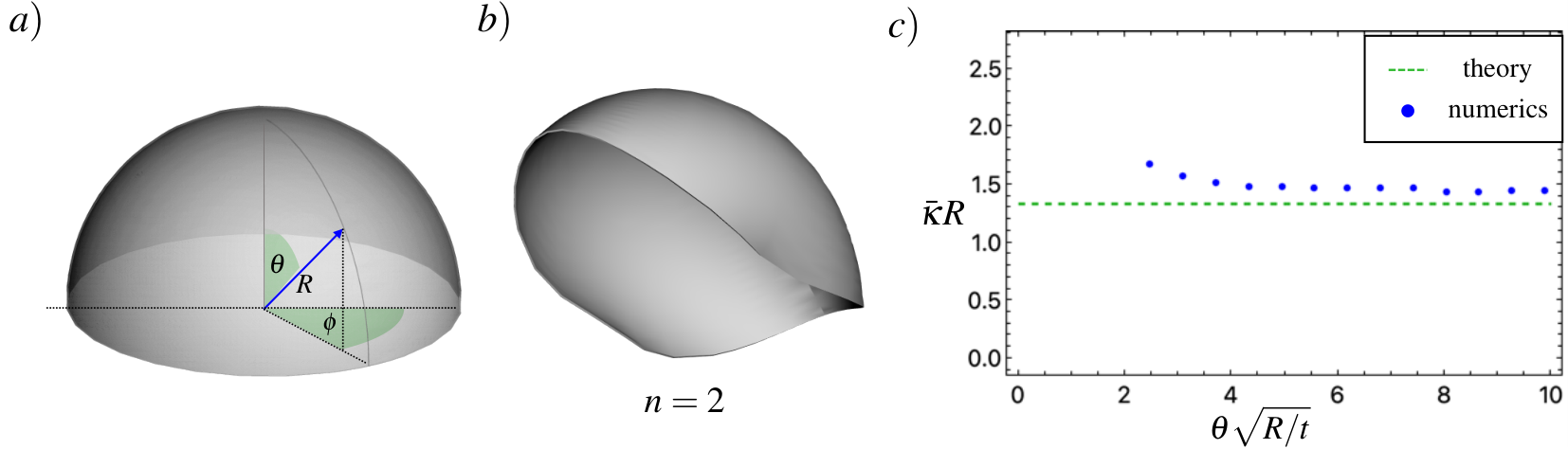
A detailed numerical and experimental study of this curvature induced instabilities in bi-layer spherical shells was recently presented by Pezzulla et. al. [41]. The authors use a combination of theoretical arguments and fitting to propose that the folding of a spherical cap with angular size $\theta_{0}$ occurs at the threshold curvature

$$\bar{\kappa}R=\frac{a}{\theta_{0}^{2}}\left(\frac{t}{R}\right)-c-\frac{b}{\pi-\theta_{0}}\sqrt{\frac{t}{R}}$$

where the parameter $a=\sqrt{10+7\sqrt{2}}$ was found by matching the theory to the flat plate case, while $b=3.6$ and $c=-0.98$ were found fitting experimental/numerical data with $\nu=0.5$. This result is more ambitious than the current work, as it aims to also capture the effect of boundary layer stretching, leading to a thickness dependent result, whereas we focus on the truly thin isometric limit. However, taking this limit of their result, in which $t/R$ vanishes, the predicted threshold would be $\bar{\kappa}=-c=0.98$, which contrasts with ours at $\bar{\kappa}R=4/3\approx 1.33$. In Fig. 5c, we compare our result with the thinnest data available in [41] ($t/R=10^{-3}$) for a range of angular depths of shell. We see an extremely encouraging level of agreement, particularly for the deeper shells. Agreement for shallower shells is actually somewhat worse because the shallow shells enter a regime where the boundary layer extent, $\sqrt{Rt}$, covers a large fraction of the shell. We thus see that shallow theory actually applies in a delicate limit where the shell is geometrically shallow, but large and thin enough that the boundary layer is still negligible.

In this paper, we have studied a simple model of instabilities in active shells that arise from the geometric incompatibility of their intrinsic and extrinsic curvatures. We have proposed a simple model, based on the requirements that the shell: (1) be geometrically shallow, (2) be thin enough to only deform isometrically, (3) has metric encoding homogeneous Gauss curvature $K$, and (4) is subject to thickness variation encoding homogeneous preferred curvature tensor ${{\bm{\bar{\kappa}}}}$. If these conditions are met, the configuration of the shell is simply given by the minimisation of the bending energy over achieved homogeneous curvature ${{\bm{\kappa}}}$, subject to the constraint that the achieved Gauss curvature is $K$.

The resultant model has three cases delineated by Gauss curvature, $K<0$, $K=0$ and $K>0$. In each case, we have given a full phase diagram showing the achieved state of the shell as a function of the prefered curvature. The phase diagrams reveal three types of curvature driven instabilities, in which the principal achieved curvatures of the shell rotate, symmetry-break and invert, as summarised in Fig. 6. The model predicts modest and thickness independent threshold-curvatures $\propto\sqrt{K}$ for all the instabilities, except inversion in the $K>0$ case, which cannot proceed isometrically, and hence has a thickness dependent threshold that diverges in the thin limit, and is beyond the reach of the simple model.

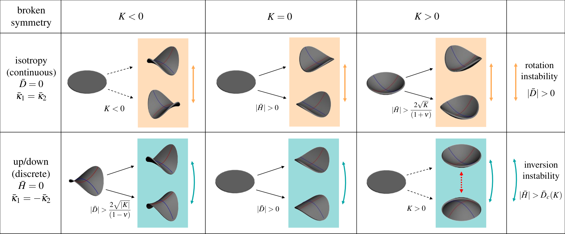
Symmetry-breaking transitions arise in two flavours. In one case, we have isotropic preferred curvature $\bar{\kappa_{1}}=\bar{\kappa_{2}}$ ($\bar{D}=0$) that is larger than permitted by the Gauss constraint, $\kappa_{1}\kappa_{2}=K$. It eventually becomes favourable for one achieved curvature to grow at the expense of the other, to better fit the preferred curvature while maintaining $K$. For $K=0$ this occurs for any finite preferred curvature, and the system rolls up in an arbitrary direction, while for $K>0$ this involves a spherical cap folding along an arbitrary direction, and occurs super-critically past a threshold preferred curvature. For $K<0$ isotropy is always broken by the shell due to the Gauss requirement to form a saddle, even when the preferred curvature is actually zero, so this type of instability is not observed by changing preferred curvatures at fixed $K<0$. However, the symmetry broken state is present, and the instability can be observed by an active change in the the metric from flat to $K<0$ [40], in which case the saddle must “decide" an orientation as it forms. Since this symmetry breaking is associated with breaking of a countinuous (rotationally invariant) symmetry, we call a continuous symmetry breaking instability.

The second symmetry-breaking case arises with equal and opposite preferred curvatures, $\bar{\kappa_{1}}=-\bar{\kappa_{2}}$ ($\bar{H}=0$) encoding a preferred symmetric saddle. In the $K=0$ case, the sheet will roll up in one of these two ways, while, for $K<0$ it will form a symmetric saddle for low preferred curvatures, and either of two asymmetric saddles beyond a threshold. The energetic motivation is the same as the continuous case, but this time a discrete up-down symmetry is broken, yielding bistability. We thus call it a discrete symmetry breaking instability. In the $K>0$ case, up-down symmetry is always broken by the Gauss requirement to have both curvatures with the same sign, but the instability can again be observed by an active change in the the metric from flat to $K>0$ [40], in which case the cap must “decide" whether to pop up or down as it forms. Curiously, breaking isotropy for $K>0$ and breaking up-down symmetry for $K<0$ are described by almost identical threshold and amplitude equations, except with $D$ and $H$ as the order parameter, and $\bar{H}$ and $\bar{D}$ as the control parameter.

The buckling threshold of symmetry breaking instabilities in both negative and positive Gauss curved systems depends on the magnitude of the preferred curvature load relative to that of the Gauss curvature. Throughout, we have discussed instabilities in terms of changing extrinsic preferred curvature, $\bar{\kappa}_{1}$ and $\bar{\kappa}_{2}$, at constant $K$, indicating active shape changes that vary through the thickness. However, one may achieve the same ends by varying $K$ at fixed $\bar{\kappa}_{1}$ and $\bar{\kappa}_{2}$ indicating active shape changes to the metric. In such a case, the shell will move along a diagonal line radiating out from the origin on any of the phase diagrams, which suffices to trigger either symmetry breaking transition by moving along the $\bar{D}=0$ and $\bar{H}=0$ axes respectively.

The rotation instabilities arise as a consequence of states that break isotropy. This angular symmetry breaking leads to Mexican-hat style energies in which the curvature frame may rotate without penalty. Applying a small bias to such a potential, by traversing the $\bar{D}=0$ line, will break the degeneracy and produce a large rotation without an energy change. All three Gauss cases have such states, and hence show rotation instabilities. Finally, the inversion instabilities arise from changing the sign of $\bar{H}$ to apply an up-down bias to the bistability generated by the discrete symmetry-breaking transitions. In this case, a finite amount of $\bar{H}$ is required to eliminate a minima, leading to a sub-critical inversion of the shell at the limit of bistability. For $K<0$ cases, this occurs at a modest thickness-independent threshold, while for $K>0$ it does not, so the instability is not present in the model, though it does occur in real shells via boundary layer stretching [41, 51].

Rotation and inversion instabilities are not naturally triggered by manipulating $K$ rather than $\bar{D}$ and $\bar{H}$, as they occur by crossing the $\bar{D}=0$ and $\bar{H}=0$ axes on the phase diagram, which no line radiating from the origin will do. However, for $K<0$, if a shell is in the local minima of the bistable region, it can exit the bistable region and invert via changes in $K$, as illustrated by the grey line in the phase diagram of Fig. 4.

The omission of stretch effects and boundary-layer mechanics underpins the simplicity of our model, but is also its key limitation. Although the boundary layer may be safely neglected in suitably thin shells, where the extent of the boundary layer, $\propto\sqrt{t}$, is negligible compared to the shell’s extent, the boundary layer is of considerable importance in many physical shells. Firstly, the boundary layer permits the $K>0$ inversion instability. Moreover, even in very thin shells, the boundary layer can allow the shape of the shell’s perimeter to couple its achieved curvature, particularly in the situations of a continuous broken symmetry; for example a Gauss flat bilayer square always rolls up along a diagonal [35, 46, 47], rather than being truly degenerate. In modest thickness shells, the boundary layer can also nucleate or delay even those instabilities which could proceed isometrically [47, 41]. However, the simple isometric model nevertheless gives considerable insight into why these instabilities occur, and when the boundary layer is a complication rather than an essential ingredient. It also clarifies when we should expect thickness independent thresholds, and is asymptotically correct at small thickness.

In contrast, the shallowness assumption in our model does not appear to be a major limitation. Indeed, we have shown that the threshold for the symmetry-breaking folding of a spherical cap subject to excessive preferred curvature is also correct for a deep spherical shell. Here the Rayleigh isometry of the sphere potentially allows a much deeper and richer exploration of the response of such a shell to excessive curvature, which we reserve for future work.

JSB is supported by a UKRI Future Leaders Fellowship, grant number MR/S017186/1. AG thanks the EPSRC for funding, project 2108804.

References

- [1] Euler L. 1744 Opera Omnia vol. I.
- [2] Yoo CH, Lee S. 2011 Stability of structures: principles and applications. Elsevier.
- [3] Zoley R. 1915 Über ein Knickproblem an der Kugelschale. PhD thesis Zurich.
- [4] Hutchinson JW. 2016 Buckling of spherical shells revisited. Proceedings of the Royal Society A: Mathematical, Physical and Engineering Sciences 472.
- [5] Kochmann DM, Bertoldi K. 2017 Exploiting microstructural instabilities in solids and structures: from metamaterials to structural transitions. Applied mechanics reviews 69.
- [6] Hirokawa Y, Tanaka T. 1984 Volume phase transition in a non-ionic gel. In AIP Conference Proceedings vol. 107 pp. 203–208. American Institute of Physics.
- [7] Klein Y, Efrati E, Sharon E. 2007 Shaping of elastic sheets by prescription of non-Euclidean metrics. Science 315, 1116–1120.
- [8] Kim J, Hanna JA, Byun M, Santangelo CD, Hayward RC. 2012 Designing responsive buckled surfaces by halftone gel lithography. Science 335, 1201–1205.
- [9] Na JH, Bende NP, Bae J, Santangelo CD, Hayward RC. 2016 Grayscale gel lithography for programmed buckling of non-Euclidean hydrogel plates. Soft Matter 12, 4985–4990.
- [10] Gladman AS, Matsumoto EA, Nuzzo RG, Mahadevan L, Lewis JA. 2016 Biomimetic 4D printing. Nature materials 15, 413–418.
- [11] Thompson DW, Thompson DW. 1942 On growth and form vol. 2. Cambridge university press Cambridge.
- [12] Savin T, Kurpios NA, Shyer AE, Florescu P, Liang H, Mahadevan L, Tabin CJ. 2011 On the growth and form of the gut. Nature 476, 57–62.
- [13] Shyer AE, Tallinen T, Nerurkar NL, Wei Z, Gil ES, Kaplan DL, Tabin CJ, Mahadevan L. 2013 Villification: how the gut gets its villi. Science 342, 212–218.
- [14] Goriely A. 2017 The mathematics and mechanics of biological growth vol. 45. Springer.
- [15] de Haan LT, Sánchez-Somolinos C, Bastiaansen CM, Schenning AP, Broer DJ. 2012 Engineering of complex order and the macroscopic deformation of liquid crystal polymer networks. Angewandte Chemie International Edition 51, 12469–12472.
- [16] Ware TH, McConney ME, Wie JJ, Tondiglia VP, White TJ. 2015 Voxelated liquid crystal elastomers. Science 347, 982–984.
- [17] Aharoni H, Xia Y, Zhang X, Kamien RD, Yang S. 2018 Universal inverse design of surfaces with thin nematic elastomer sheets. Proceedings of the National Academy of Sciences 115, 7206–7211.
- [18] Barnes M, Verduzco R. 2019 Direct shape programming of liquid crystal elastomers. Soft matter 15, 870–879.
- [19] Siéfert E, Reyssat E, Bico J, Roman B. 2019 Bio-inspired pneumatic shape-morphing elastomers. Nature materials 18, 24–28.
- [20] Warner M, Siéfert E. 2020 Inflationary routes to Gaussian curved topography. Proc. R. Soc. A 476, 20200047.
- [21] Mosadegh B, Polygerinos P, Keplinger C, Wennstedt S, Shepherd RF, Gupta U, Shim J, Bertoldi K, Walsh CJ, Whitesides GM. 2014 Pneumatic networks for soft robotics that actuate rapidly. Advanced functional materials 24, 2163–2170.
- [22] Bowden N, Brittain S, Evans AG, Hutchinson JW, Whitesides GM. 1998 Spontaneous formation of ordered structures in thin films of metals supported on an elastomeric polymer. nature 393, 146–149.
- [23] Jiang H, Khang DY, Song J, Sun Y, Huang Y, Rogers JA. 2007 Finite deformation mechanics in buckled thin films on compliant supports. Proceedings of the National Academy of Sciences 104, 15607–15612.
- [24] Sultan E, Boudaoud A. 2008 The buckling of a swollen thin gel layer bound to a compliant substrate. Journal of applied mechanics 75.
- [25] Huang Z, Hong W, Suo Z. 2005 Nonlinear analyses of wrinkles in a film bonded to a compliant substrate. Journal of the Mechanics and Physics of Solids 53, 2101–2118.
- [26] Audoly B, Boudaoud A. 2007 Buckling of a thin film bound to a compliant substrate (part I). Formulation, linear stability of cylindrical patterns, secondary bifurcations. Submitted to Journal of the Mechanics and Physics of Solids.
- [27] Tallinen T, Chung JY, Rosseau F, Girard N, Lefevre J, Mahadevan L. 2016 On the growth and form of cortical convolutions. Nature Phys. 12, 588–593.
- [28] Tallinen T, Chung JY, Biggins JS, Mahadevan L. 2014 Gyrification from constrained cortical expansion. PNAS 111, 12667–12672.
- [29] Shyer AE, Tallinen T, Nerurkar NL, Wei Z, Gil ES, Kaplan. DL, Tabin CJ, Mahadevan L. 2013 Villification: How the Gut Gets Its Villi. Science 342, 212–218.
- [30] Savin T, Kurpios NA, Shyer AE, Florescu P, Liang H, Mahadevan L, Tabin CJ. 2011 On the growth and form of the gut. Nature 476, 57–63.
- [31] Forterre Y, Skotheim JM, Dumais J, Mahadevan L. 2005 How the Venus flytrap snaps. Nature 433, 421–425.
- [32] Katifori E, Alben S, Cerda E, Nelson DR, Dumais J. 2010 Foldable structures and the natural design of pollen grains. Proceedings of the National Academy of Sciences of the United States of America 107, 7635–7639.
- [33] Couturier E, Dumais J, Cerda E, Katifori E. 2013 Folding of an opened spherical shell. Soft Matter 9, 8359–8367.
- [34] Božič A, Šiber A. 2020 Mechanical design of apertures and the infolding of pollen grain. Proceedings of the National Academy of Sciences of the United States of America 117, 26600–26607.
- [35] Seffen K, Pellegrino S. 1999 Deployment dynamics of tape springs. Proceedings of the Royal Society of London. Series A: Mathematical, Physical and Engineering Sciences 455, 1003–1048.
- [36] Kühnel W. 2015 Differential geometry vol. 77. American Mathematical Soc.
- [37] van Rees WM, Vouga E, Mahadevan L. 2017 Growth patterns for shape-shifting elastic bilayers. Proceedings of the National Academy of Sciences 114, 11597–11602.
- [38] Warner M. 2020 Topographic mechanics and applications of liquid crystalline solids. Annual Review of Condensed Matter Physics 11, 125–145.
- [39] Timoshenko S. 1925 Analysis of bi-metal thermostats. Josa 11, 233–255.
- [40] Efrati E, Sharon E, Kupferman R. 2009 Elastic theory of unconstrained non-Euclidean plates. Journal of the Mechanics and Physics of Solids 57, 762–775.
- [41] Pezzulla M, Stoop N, Steranka MP, Bade AJ, Holmes DP. 2018 Curvature-Induced Instabilities of Shells. Physical Review Letters 120, 48002.
- [42] Pandey A, Moulton DE, Vella D, Holmes DP. 2014 Dynamics of snapping beams and jumping poppers. EPL (Europhysics Letters) 105, 24001.
- [43] Mansfield EH. 1989 The bending and stretching of plates.
- [44] Kebadze E, Guest S, Pellegrino S. 2004 Bistable prestressed shell structures. International Journal of Solids and Structures 41, 2801–2820.
- [45] Pezzulla M, Smith GP, Nardinocchi P, Holmes DP. 2016 Geometry and mechanics of thin growing bilayers. Soft Matter 12, 4435–4442.
- [46] Pezzulla M, Stoop N, Jiang X, Holmes DP. 2017 Curvature-driven morphing of non-Euclidean shells Subject Areas :. Proceedings of the Royal Society A: Mathematical, Physical and Engineering Sciences.
- [47] Jiang X, Pezzulla M, Shao H, Ghosh TK, Holmes DP. 2018 Snapping of bistable, prestressed cylindrical shells. Epl 122.
- [48] Sawa Y, Ye F, Urayama K, Takigawa T, Gimenez-Pinto V, Selinger RL, Selinger JV. 2011 Shape selection of twist-nematic-elastomer ribbons. Proceedings of the National Academy of Sciences 108, 6364–6368.
- [49] Efrati E, Irvine WT. 2014 Orientation-dependent handedness and chiral design. Physical Review X 4, 011003.
- [50] Gao J, Clement A, Tabrizi M, Shankar MR. 2021 Molecularly Directed, Geometrically Latched, Impulsive Actuation Powers Sub-Gram Scale Motility. Advanced Materials Technologies p. 2100979.
- [51] Taffetani M, Jiang X, Holmes DP, Vella D. 2018 Static bistability of spherical caps. arXiv.
- [52] Strutt JW, Rayleigh JWSB. 1894 The theory of sound vol. 1. Macmillan.