Time-Range FDA Beampattern Characteristics Note: This work was supported in part by National Natural Science Foundation of China 62171092, in part by Sichuan Science and Technology Program under grant 2018RZ0141, and in part by the Swedish SRA ESSENCE (grant no. 2020 6:2). Journal: arXiv
Abstract
Current literature show that frequency diverse arrays (FDAs) are able of producing range-angle-dependent and time-variant transmit beampatterns, but the resulting time and range dependencies and their characteristics are still not well understood. This paper examines the FDA transmission model and the model for the FDA array factor, considering their time-range relationship. We develop two FDA transmit beampatterns, both yielding the auto-scanning capability of the FDA transmit beams. The scan speed, scan volume, and initial mainlobe direction of the beams are also analyzed. In addition, the equivalent conditions for the FDA integral transmit beampattern and the multiple-input multiple-output (MIMO) beampattern are investigated. Various numerical simulations illustrate the auto-scanning property of the FDA beampattern and the proposed equivalent relationship with the MIMO beampattern, providing the basis for an improved understanding and design of the FDA transmit beampattern.
Keywords:
Frequency diverse array (FDA), transmit beampattern, time-variant beampattern, auto-scanning capability, range-time relations1 Introduction
The concept of a frequency diverse array (FDA) was first proposed in 2006 2006Frequency, and was patented by Wicks and Antonik in 2008Frequency. As compared to a phased-array, FDA employs different carrier frequencies across the array elements to generate a transmit beampattern which is a function of the range, angle, and time 2008Frequenc, 2009Developments, jia2023waveform. This interesting fusion of frequency and spatial diversities provides FDA with broad application prospects and the topic has attracted notable interest since wang2016moving, 9161264, 9440819, 9944910. As the standard FDA usually produces an S-shaped beampattern in the range-angle plane jia2023joint, logarithmic 6951408, time-modulated 2014Frequency, 2016Range, random 2017The, and optimized 2016Frequency frequency offsets (FOs) have been suggested to decouple the beampattern. Combining co-located multiple-input multiple-output (MIMO) with waveform diversity li2007mimo, distributed MIMO with spatial diversity haimovich2007mimo, a focused transmit beampattern has also been synthesized by optimizing the transmitted baseband waveform 2013Frequency. Furthermore, to obtain the desired dot-shaped time-invariant beampattern, the alternating direction method of multipliers (ADMM) algorithm was adopted to design the transmitted weight matrix in 2021Transmit. On the other hand, multiple methods have been proposed to explore the range-angle-dependent property of the FDA transmit beampattern, such as dual-pulse FDA 2014Rge, FDA-MIMO 2014Transmit, and FDA subarrays 2014Subarray. Basit et al 2019Rnge studied the use of FDA with nonlinearly progressive FOs for joint radar and communication functionalities. Xu et al. proposed an FDA strategy for identifying and suppressing deceptive mainlobe interference and for suppressing range-ambiguous clutter 2015Deceptive, which was shown to yield better performance than that of a phased-array 7181636. Additionally, the use of FDA for low probability of intercept (LPI) transmit beamforming 2016Overview, 2017Cognitive, secure communications 2016Artificial, and target detection 9212375 have been reported.
Since the angle-time coupling is the aspect of an FDA antenna that differs it from a conventional phased-array or MIMO systems, it is more meaningful to effectively utilize the time variance to improve the performance than to strive to decouple the beampattern. It is not only that the FDA antenna’s time-variant property cannot be adequately suppressed, but the obtained pseudo-static or focused FDA would lose its advantage in comparison to phased-array and MIMO antennas. The time variance of the FDA transmit beampattern was analyzed in 2020Enhanced and 8074796, but the time-range relations are still not sufficiently detailed.
In this paper, considering its time-range dependencies, an accurate model of the FDA instantaneous transmit beampattern (FITB) is formulated and then used to detail the auto-scanning capability of an FDA transmit beam. Auto-scanning here refers to autonomously and continuously changing the direction of the mainlobe of the beam within the pulse duration without electronically adjusting the phase shifters. The scan speed, scan volume, and initial mainlobe direction of the beam are also detailed. Comparing the resulting beampattern with that of a phased-array, it can be seen that the uniform linear FO is the optimal choice for FDA. In addition, we present the FDA integral transmit beampattern model (FGTB), which provides a method to calculate the amount of energy radiated by the FDA to a certain azimuth angle during the pulse duration. The relation between the FGTB and the MIMO beampatterns are also investigated, revealing the conditions for equivalence for these systems.
The remaining sections are organized as follows. Section 2 reformulate the FDA transmitted electric field model considering the underlying time-range dependencies. In Section 3, the proposed FITB is derived and its scan speed, scan volume, and initial mainlobe direction are derived. In Section 4, the influence of the FO on the proposed FITB and the relationship between the FDA and a phased-array are discussed. Next, the FGTB model is derived in Section 5, followed by a comparison with the MIMO beampattern. Finally, conclusions are drawn in Section 6.
2 Signal Model

The transmitted electric field at a given far-field point target for a range-angle pair with the target slant range , using the first element as the reference, is the sum of the field components radiated by the individual FDA elements, as illustrated in Fig. 1, such that 7740083
| (1) |
for , where is the beamformer weight of the -th element with denoting the number of transmit elements. Furthermore, represents the radiation pattern of the -th element evaluated at its carrier frequency , denotes the slant range from the -th element to the target, the factor accounts for the free space loss, and is the baseband complex waveform with unit energy, i.e., , where and are the pulse duration and the conjugate operators, respectively. It is reasonable to assume that the radiation patterns are nearly the same within the FDA’s transmission bandwidth, i.e., , where is the center carrier frequency. In addition, under far-field conditions, since , it may be assumed that the distance attenuation has an identical influence on the electric field amplitudes of all array elements. Therefore, the FDA transmitted electric field can be well modeled as
| (2) |
for , where based on the narrowband assumption
| (3) |
with being the bandwidth of the baseband envelope . In order to admit to a closed-form representation, uniform linear frequency increments are adopted (the effect of nonlinear FO on the beampattern will be analyzed in Section 4, i.e.,
| (4) |
for , where denotes the FO. Then, the FDA transmitted electric field can be reformulated as
| (5) | ||||
for , where , , and denote the transpose, conjugate transpose, and Hadamard operators, respectively, and
| (6a) | |||
| (6b) | |||
| (6c) | |||
| (6d) |
Using uniform weighting, i.e., , the FDA array factor can be rewritten as wang2013range, 2016Frequency, 2016Fruency, 2021Transmit
| (7) | ||||
where the approximation
| (8) |
for , has been used. One observes from (7) that, different from phased-arrays, the obtained array factor features an additional dependence on the range and the time as well as the angle, a property which renders the field of an FDA different from that of a phased-array. However, the range of the time variable , , is inadvertently ignored in (7). In order to fully explore the characteristics of the beampattern, one may use the variable substitution , yielding
| (9) |
where
| (10) |
for . It must be emphasized that the time uniqueness should be guaranteed. For a given target distance, the trip delay is constant. It may be noted from (9) that the new array factor formulation is time-angle-dependent within the pulse duration, which also exhibits a considerable difference from the static beampattern (array factor) of a conventional phased-array. As the array factor is time-variant, we here term this the FDA instantaneous transmit beampattern (FITB). However, it is worth noting that the range-dependent property proposed in 2016Frequency, 2016Fruency, 2021Transmit will not hold for the FDA transmit beampattern.
Current research on the FDA transmit beampattern mainly focuses on the static range-angle-dependent beampattern by fixing the time variable at the instantaneous moment in (7), see, e.g., 2014Frequency, 2016Range, 2017Sutions. As alternatives, the focused transmit beampatterns in the range-angle plane has also been synthesized using designed logarithmic 6951408, time-modulated 2014Frequency, 2016Range, random 2017The, or optimized 2016Frequency FOs. However, the range-dependent theory of the FDA beampatterns was challenged by the consideration of the Huygens-Fresnel principle urone1998college. Since the time variable belongs to , the conclusion of a range-dependent array factor is not convincing, This in turn implies that the characteristics of the FDA transmit beampattern are still in need of further clarification.
3 the characteristics of FITB
3.1 Zero-time Cut
Although the proposed FITB is time-variant, it is still meaningful to analyze its characteristics at a given time instant. When in (9), the zero-time cut of FITB can be expressed as
| (11) |
where the zero-time cut refers to the beampattern at the instantaneous moment . This can be understood as the electric field radiated by the FDA antenna elements combine in phase at this time. Then, the first null beamwidth, i.e., the mainbeam width, is
| (12) |
with its peak being located at
| (13) |
where denote the integer set. Fig. 2 shows the zero-time cut of the FITB, using , , and . It may be seen that the larger the inter-element spacing , the narrower the beamwidth is. If exceeds half the reference wavelength , the grating lobes will appear around .

3.2 Auto-scanning
According to (9), the FITB has peaks at locations satisfying
| (14) |
for and . Therefore, the mainbeam at time instant will be equivalently steered to direction
| (15) |
Taking the derivative of both sides of (15) with respect to , the spatial scan speed of FITB can be obtained as
| (16) | ||||
Furthermore, the beamwidth or resolution of the field at a given time instant satisfies
| (17) | ||||
Adopting the convenient 4-dB Rayleigh width criterion, selecting in (17), yields
| (18) |
It may be noted that relates to the effective angular extension of the field, being linked to the azimuth resolution as
| (19) | ||||
implying that
| (20) |
From (16) and (20), one may conclude that
- 1)
Since a delay increment along the azimuth dimension does not translate to a relative phase difference for identical sources, evidenced by the lack of any radial gradients along the time axis for , a phased-array can only control the direction of the mainlobe by electronically adjusting the phase shifters. The generated field is therefore static, exhibiting maxima (minima) when the radiated element fields add constructively (destructively). However, due to the existence of FO, the phase progression between the FDA elements grows in time, such that the auto-scanning behavior occurs without any phase shifters. Since is a decreasing function, the scan speed is nonlinear, directly proportional to the FO and the current azimuth angle. This auto-scanning ability allows the beam to spend more time at boresite and less at extreme angles, which can be quite useful in practical applications.
- 2)
The resolution of the beam is time-invariant. Within the pulse duration, the beam coverage (scan volume) is
(21) which is thus dependent on the FO and the pulse duration . In particular, if , the FDA can scan through the whole visible azimuth sector within one pulse duration. As a result, the presence of a small FO enables the FDA to transmit automatically scanning beams.
3.3 Initial Mainlobe Direction
For phased arrays, the transmit weight vector ensures that the transmit beam is steered in the desired direction. However, due to the auto-scanning capability of the FDA beam, the vector will mainly affect the initial mainlobe direction. For example, setting as
| (22) |
and substituting (22) into (5) yields
| (23) | ||||
Thus, the weight-dependent FITB at can be expressed as
| (24) |
with its peak appearing at .
3.4 Numerical Simulation
In this section, various numerical simulations are presented to evaluate the auto-scanning behavior of the FDA transmitted beampattern. For a given far field distance, we first verify the relationship between the FO and the beam scan volume. Then, we examine the angular extension of the beam over different time periods. Next, we illustrate the effect of the transmit weight vector on the initial mainlobe direction of the beam. Finally, to explain the difference between the range dependent characteristics used in 2014Frequency, 2014Rge, 2016Frequency, 2017Joint, 2017The and that of the auto-scanning property proposed in this paper, these two beampatterns are compared, at two different far-field distances. In all simulations, we assumed that the number of FDA transmit array elements is , the reference carrier frequency is , and that the inter-element spacing is (for a phased-array this implies ). For simplicity, a rectangular pulse with pulse duration is considered as the baseband waveform.
3.4.1 Scan volume
Fig. 3 illustrates the simulated FDA electric fields for different FO configurations using a uniform weight vector, at a given far-field distance , with the field of the phased-array () acting as a benchmark. It can be seen that for a phased-array, the field is static, i.e., it is not spatially scanned over time. Unlike for a phased-array, the field formed by the FDA is dynamic. Small FO produces limited beam coverage, almost the same as the phased-array field, although the scan volume becomes larger as the FO increases. The results also show that the FDA can scan the entire visible azimuth sector within one pulse duration when the FO satisfies , corresponding to the results in Fig. 3(c). This observation agrees with the results discussed in Section 3.2. It can also be found that if the FO is larger than , the FDA is sufficient to scan through the entire visible azimuth sector multiple times within one pulse period. As shown in Fig. 3(d), for this example, the beam scans the entire sector twice. It is worth reiterating that the auto-scanning behavior of the FDA occurs without any phase shifters. However, as compared to the phased-array, the radiated energy is also dispersed in the entire observed airspace, which will inevitably lead to a loss of transmission gain.


3.4.2 Scan speed
Evidenced by the derivation in (15), the beam scanning is nonlinear with time. Fig. 4 shows the energy distribution of the FDA along the azimuth dimension for the same duration () at the far-field distance , where the resulting scan time in Fig. 4(a) and Fig. 4(b) are and , respectively. Here, a uniform weight vector has been used, with the FO being set to . In the figure, the black straight lines mark the mainbeam extension. One may note from Fig. 4 that, despite having the same duration, Fig. 4(b) exhibits a larger beam coverage than Fig. 4(a). To be more precise, the beam coverage is about in Fig. 4(a), and in Fig. 4(b). The reason for this is that wider beam coverage results in faster scans over time, a result that is consistent with the derivation in (16).


3.4.3 Initial mainlobe direction
As shown, a uniform transmit weight vector causes the beam to scan from an azimuth of . Fig. 5 illustrates the resulting beampatterns for different weight vectors, where the FO is . Here, the transmit weight vector is set to in Fig. 5(a), and to in Fig. 5(b). As expected, the mainbeam starts scanning from the and , respectively, indicating that the simulation results are consistent with results discussed in Section 3.3.


3.4.4 Beampatterns at different distances
Existing studies using the array factor represented by (7) blur the relationship between time and range, holding that the FDA transmit beampattern is not only a function of time, but also a function of the target distance. However, as our proposed FITB in (9) shows, it is angle-time-dependent but not range-dependent. Fig. 6 compares the beampatterns formed by the FDA array factors in (7) and the proposed FITB given in (9), for the case when the same transmitted pulse travels to a range of and , respectively, with the FO set to . Comparing Figs. 6(a) and 6(c), the simulation results of Figs. 6(b) and 6(d) reveal that when the same pulse propagates to different distances in free space, the direction of the mainlobe of the beam formed by the FDA changes. This phenomenon clearly violates the law of electromagnetic wave propagation. Furthermore, as can be seen from Figs. 6(a) and 6(c), for a given distance in free space, the FDA beam automatically scans along the azimuth dimension for the duration of the pulse. Then, the identical auto-scanning process propagates forward at the speed of light. In conclusion, our proposed FITB model is deemed to be more accurately representing the actual FDA beam transmission process than the one presented in (7).


4 FDA and phased-array
Considering the range-time-angle-dependent array factor in (7), most conventional studies typically concentrate on designing FOs striving to decouple the time-variant transmit beampattern 2014Subarray, 2016Frequency. A significant transmission gain can then be obtained by focusing the energy on the desired target in the range-angle space. However, by analyzing the relationship between distance and time, it can be seen that the FDA transmit beam has auto-scanning properties. In this sector, the influence of FO on the proposed FITB and the relationship between the FDA and the phased-array will be discussed.
4.1 Different FOs
As the beampattern formed by the linear FO can be expressed in closed-form, its characteristics is possible to analyze in detail, with even nonlinear FOs, such as logarithmic 6951408 FO and random 2017The FO, having been investigated in the FDA literature. Consider the nonlinear FOs , for which the electric field can be expressed as
| (25) | ||||
for . Then, the FITB can be expressed as
| (26) |
where
| (27a) | |||
| (27b) |
Similarly, for time-dependent or time-modulated FOs 2014Frequency, shao2016time, yao2016solutions, yao2016synthesis. the FITB has the form
| (28) |
for , where
| (29) |
where , is a function of , such as , , , or yao2016solutions, yao2016synthesis.
4.2 FDA and phased-array
In general, FDA can be regarded as a phased-array with time-variant weight vector. If the weight vector
| (30) |
an auto-scanning transmit beam with zero initial direction will be generated. Applying a time-variant weight vector in FDA, the FITB can be approximated as
| (31) |
for , where is a slowly varying phase function. The function in (31) has peaks at locations satisfying
| (32) |
for . Note that any desired beam scanning scheme can be realized by appropriately designing . For example, if one expect the beam to be steered to at and to at , one can for and , set
| (33) |
whereas for and ,
| (34) |
At other times and angles, one sets
| (35) |
Interestingly, the array system designed in this scheme is very similar to the traditional phased-array, while it has only a weak connection to FDA. Generally, phased-arrays use fixed transmit weights to steer the beam in the desired direction, whereas the designed array uses time-variant weights within the desired steering interval. This also illustrates how the FDA solution to achieve the desired beam steering makes the designed array system converge to the time-variant phased-array, suggesting that using a uniform FO is the optimal choice for the FDA transmit beampattern. We also note that a uniform FO can be realized using direct digital synthesis (DDS) technology cordesses2004directtt.
4.3 Numerical Simulation
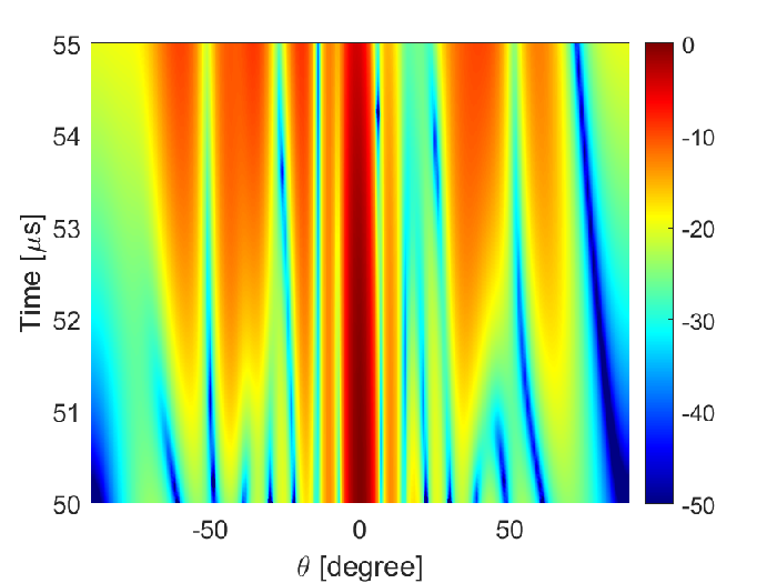


We proceed to consider the FDA simulation parameters detailed in Section 3.4. Fig. 7 depicts the FITB for different types of FOs, including the random 2017The, Costas-coded wang2016range, logarithmic 6951408, and square FOs yao2016synthesis. The FOs used above are widely used to design the FDA transmit beampattern focused in the range-angele domain. It may be seen that whether configured with nonlinear FOs or time-modulated FOs, the resulting FDA always produces a beampattern with its mainlobe focusing in the initial direction (in these simulation, the uniform weight vector results in the beam steering to azimuth ), similar to the static beampattern of a phased-array. This is due to the fact that the FDA using these FOs will generate a focused beampattern without considering the range-time relationship. Therefore, the range-time relationship will appear to be static (approximatively).
5 FDA integral transmit beampattern
As the proposed FITB is time-dependent, it may be viewed as obtaining all the energy radiated to a certain azimuth during the pulse duration, i.e., as a FDA integral transmit beampattern (FGTB), defined as
| (36) | ||||
where
| (37a) | |||
| (37b) |
and
| (38) |
denotes the covariance matrix of the FDA transmitted signal, with being the trace operator, and
| (39) |
is the baseband waveform vector, with , denoting the baseband envelope of the -th array element. This implies that the FGTB can be considered as the result of integrating the proposed FITB over the entire pulse duration. For a co-located MIMO array, the FGTB transmit beampattern li2007mimo, liii2008mimo can be expressed as
| (40) |
where denotes the covariance matrix of the MIMO waveform vector . It is worth noting that the derived FGTB has a form consistent with the conventional MIMO radar beampattern. The only difference is in the steering vectors and . Consider that the MIMO and FDA transmit signals can be expressed as
| (41) |
and
| (42) |
respectively. Therefore, if the contribution of the FO-dependent steering vector can be neglected in FGTB, the problem of FGTB synthesis based on waveform optimization is equivalent to the beampattern design of co-located MIMO. Then, by replacing the designed waveform equivalently with the FDA transmit waveform, massive MIMO transmit beampattern design techniques (see, e.g., stoica2007probing, ahmed2014mimo, zhang2015mimo, aubry2016mimo) can be applied to the FGTB synthesis in parallel. Notably, if
| (43) |
for , the contribution of the vector to the FGTB can be neglected. Combined with the narrowband assumption in (3), the FO is required to satisfy the condition
| (44) |
for . Therefore, the FO-dependent steering vector should be taken into account for scenarios with large array apertures and high range resolution requirements. In particular, this holds for FDA-MIMO systems sammartino2013frequency, 7181636, as their configuration requires that each element transmits the baseband waveforms with non-overlapping spectra, i.e., . In this case, the FOs will not meet the requirements in (44), and FO effects must be considered.
It is interesting to examine two extreme cases, for which the properties of the FGTB can be explained analytically. For , , the FGTB can be approximately expressed as
| (45) |
which is thus similar to the beampattern of a coherent MIMO array. For , with denoting the identity matrix, the FGTB can be approximated as
| (46) |
where denotes the norm, indicating that the FGTB acts in a omnidirectional manner, corresponding to an orthogonal MIMO beampattern.
5.1 Numerical Simulation
5.1.1 FGTB
Fig. 8 depicts the FGTB, where the bandwidth of the baseband waveform transmitted by each array element is , with the remaining simulation parameters being same as in Section 3.4.

It is noted that as the FO increases, the coherent gain decreases, whereas the mainlobe width of the beam grows. For , the transmitted waveforms are orthogonal, resulting in an omnidirectional energy radiation, such that the coherent gain does not exist. These results can also be explained from the perspective of beam scanning as analyzed in Section 3.4. For small FOs, the beam coverage is negligible during the pulse duration, so the FGTB is similar to the conventional coherent MIMO array. That is, there will be a clear peak at azimuth . When , the FDA scans though the whole visible azimuth sector within one pulse duration, which corresponds to the omnidirectional FGTB in (44).
5.1.2 The influence of the FO on the FGTB
To achieve the transmit waveform analogy for a co-located MIMO, a chirp signal with an additional uniform FOs is depolyed. Then, the basedband waveform transmitted by the -th element of the MIMO array can be written as
| (47a) |
where
| (48) |
and , for , denotes the chirp rate of the th waveform. For FDA, the -th baseband waveform is
| (49) |
It should be emphasized that, for MIMO, the beampattern is calculated based on (40), while for FDA, the calculation is based on (36). As an example, consider a case with transmit array elements, with all other simulation parameters are as given in 3.4. Fig. 9 shows the simulation of the FGTB and the co-located MIMO beampatterns, where the reference bandwidth is . As can be seen in Fig. 9(a), in the case of uniform weights and a small FO, the beampattern still has a clear peak at azimuth . The increase in FO causes the coherence of the transmitted waveform to decrease, resulting in a gradually flat beampattern and the disappearance of peaks. As shown in Fig. 9(b), this condition exists regardless of the transmit weights. Most importantly, it can still be clearly observed that there is no obvious difference between the FGTB and MIMO beampatterns regardless of FOs being small or large (the curves overlap). This shows that theoretically, although the large FO does not satisfy the equivalent conditions in (44), the two beampatterns are equivalent. In fact, this reveals that the FDA can be regarded as a MIMO radar for which the phase change is caused by the FO. However, the resulting phase has a negligible effect on the energy distribution at a given location in free space, as expected for the proposed FGTB. At the same time, if the energy distribution of the whole space is considered, the presence of FOs causes the beam to automatically scan, which corresponds to the proposed FITB.


6 Conclusion
In this paper, the time-range characteristics of the FDA transmit beampattern has been detailed.
Two FDA transmit beampattern models, namely, the instantaneous transmit beampattern and the integral transmit beampattern, have been formulated and analyzed.
Numerical simulations show that the presence of a small FO gives the FDA the ability to transmit scanning beams automatically.
Furthermore, we show that the often made assumption of range-angle-time dependent FDA transmit beampattern is not accurate.
In addition, it is shown that the FO-dependent steering vector constitutes the only difference between the proposed FGTB and the MIMO beampattern, creating a better understanding of the FDA range-time relations.
References
- [1] Paul Antonik, Michael C Wicks, Hugh D Griffiths, and Christopher J Baker. Frequency diverse array radars. In 2006 IEEE Conference on Radar, pages 3–pp. IEEE, 2006.
- [2] Michael C Wicks and Paul Antonik. Method and apparatus for a frequency diverse array, March 31 2009. US Patent 7,511,665.
- [3] Jingjing Huang, Kin-Fai Tong, and CJ Baker. Frequency diverse array with beam scanning feature. In 2008 IEEE Antennas and Propagation Society International Symposium, pages 1–4. IEEE, 2008.
- [4] PF Sammartino and CJ Baker. Developments in the frequency diverse bistatic system. In 2009 IEEE Radar Conference, pages 1–5. IEEE, 2009.
- [5] Wenkai Jia, Andreas Jakobsson, and Wen-Qin Wang. Waveform optimization with SINR criteria for FDA radar in the presence of signal-dependent mainlobe interference. Signal Processing, 204:108851, 2023.
- [6] Wen-Qin Wang. Moving-target tracking by cognitive RF stealth radar using frequency diverse array antenna. IEEE Transactions on Geoscience and Remote Sensing, 54(7):3764–3773, 2016.
- [7] Lan Lan, Jingwei Xu, Guisheng Liao, Yuhong Zhang, Francesco Fioranelli, and Hing Cheung So. Suppression of mainbeam deceptive jammer with FDA-MIMO radar. IEEE Transactions on Vehicular Technology, 69(10):11584–11598, 2020.
- [8] Lan Lan, Massimo Rosamilia, Augusto Aubry, Antonio De Maio, and Guisheng Liao. Single-snapshot angle and incremental range estimation for FDA-MIMO radar. IEEE Transactions on Aerospace and Electronic Systems, 57(6):3705–3718, 2021.
- [9] Wenkai Jia, Andreas Jakobsson, and Wen-Qin Wang. Designing FDA radars robust to contaminated shared spectra. IEEE Transactions on Aerospace and Electronic Systems, pages 1–13, 2022.
- [10] Wenkai Jia, Wen-Qin Wang, and Shunsheng Zhang. Joint design of the transmit and receive weights for coherent FDA radar. Signal Processing, 204:108834, 2023.
- [11] Waseem Khan, Ijaz Mansoor Qureshi, and Sarah Saeed. Frequency diverse array radar with logarithmically increasing frequency offset. IEEE antennas and wireless propagation letters, 14:499–502, 2014.
- [12] Waseem Khan and Ijaz Mansoor Qureshi. Frequency diverse array radar with time-dependent frequency offset. IEEE Antennas and Wireless Propagation Letters, 13:758–761, 2014.
- [13] Wasim Khan, Ijaz Mansoor Qureshi, Abdul Basit, and Waseem Khan. Range-bins-based MIMO frequency diverse array radar with logarithmic frequency offset. IEEE Antennas and Wireless Propagation Letters, 15:885–888, 2015.
- [14] Y. Liu, R. Hang, L. Wang, and A. Nehorai. The random frequency diverse array: A new antenna structure for uncoupled direction-range indication in active sensing. IEEE Journal of Selected Topics in Signal Processing, 11(2):295–308, 2017.
- [15] Jie Xiong, Wen-Qin Wang, Huaizong Shao, and Hui Chen. Frequency diverse array transmit beampattern optimization with genetic algorithm. IEEE Antennas and Wireless Propagation Letters, 16:469–472, 2016.
- [16] Jian Li and Petre Stoica. MIMO radar with colocated antennas. IEEE Signal Processing Magazine, 24(5):106–114, 2007.
- [17] Alexander M Haimovich, Rick S Blum, and Leonard J Cimini. MIMO radar with widely separated antennas. IEEE Signal Processing Magazine, 25(1):116–129, 2007.
- [18] P. F. Sammartino, C. J. Baker, and H. D. Griffiths. Frequency diverse MIMO techniques for radar. IEEE Transactions on Aerospace and Electronic Systems, 49(1):201–222, 2013.
- [19] Abdul Basit, Wen-Qin Wang, Samad Wali, and Shaddrack Yaw Nusenu. Transmit beamspace design for FDA-MIMO radar with alternating direction method of multipliers. Signal Processing, 180:107832, 2021.
- [20] W. Q Wang and H. Shao. Range-angle localization of targets by a double-pulse frequency diverse array radar. IEEE Journal of Selected Topics in Signal Processing, 8(1):106–114, 2014.
- [21] W. Q. Wang and H. C. So. Transmit subaperturing for range and angle estimation in frequency diverse array radar. IEEE Transactions on Signal Processing, 62(8):2000–2011, 2014.
- [22] W. Q Wang. Subarray-based frequency diverse array radar for target range-angle estimation. Aerospace & Electronic Systems IEEE Transactions on, 50(4):3057–3067, 2014.
- [23] A. Basit, W. Q. Wang, S. Y. Nusenu, and S. Zhang. Range-angle-dependent beampattern synthesis with null depth control for joint radar communication. IEEE Antennas and Wireless Propagation Letters, 18(9):1741–1745, 2019.
- [24] Jingwei Xu, Guisheng Liao, Shengqi Zhu, and Hing Cheung So. Deceptive jamming suppression with frequency diverse MIMO radar. Signal Processing, 113:9–17, 2015.
- [25] Jingwei Xu, Shengqi Zhu, and Guisheng Liao. Range ambiguous clutter suppression for airborne FDA-STAP radar. IEEE Journal of Selected Topics in Signal Processing, 9(8):1620–1631, 2015.
- [26] W. Q. Wang. Overview of frequency diverse array in radar and navigation applications. IET Radar Sonar & Navigation, 10(6):1001–1012, 2016.
- [27] J. Xiong, W. Q. Wang, C. Cui, and K. Gao. Cognitive FDA-MIMO radar for LPI transmit beamforming. IET Radar Sonar & Navigation, 11(10):1574–1580, 2017.
- [28] Jinsong Hu, Shihao Yan, Feng Shu, Jiangzhou Wang, Jun Li, and Yijin Zhang. Artificial-noise-aided secure transmission with directional modulation based on random frequency diverse arrays. IEEE Access, 5:1658–1667, 2017.
- [29] Lan Lan, Angela Marino, Augusto Aubry, Antonio De Maio, Guisheng Liao, Jingwei Xu, and Yuhong Zhang. GLRT-based adaptive target detection in FDA-MIMO radar. IEEE Transactions on Aerospace and Electronic Systems, 57(1):597–613, 2021.
- [30] Yanhong Xu and Kwai-Man Luk. Enhanced transmit–receive beamforming for frequency diverse array. IEEE Transactions on Antennas and Propagation, 68(7):5344–5352, 2020.
- [31] Ronghua Gui, Wen-Qin Wang, Can Cui, and Hing Cheung So. Coherent pulsed-FDA radar receiver design with time-variance consideration: Sinr and crb analysis. IEEE Transactions on Signal Processing, 66(1):200–214, 2018.
- [32] Wen-Qin Wang, Hing Cheung So, and Alfonso Farina. An overview on time/frequency modulated array processing. IEEE Journal of Selected Topics in Signal Processing, 11(2):228–246, 2017.
- [33] Wen-Qin Wang. Range-angle dependent transmit beampattern synthesis for linear frequency diverse arrays. IEEE transactions on antennas and propagation, 61(8):4073–4081, 2013.
- [34] A-Min Yao, Wen Wu, and Da-Gang Fang. Frequency diverse array antenna using time-modulated optimized frequency offset to obtain time-invariant spatial fine focusing beampattern. IEEE Transactions on Antennas and Propagation, 64(10):4434–4446, 2016.
- [35] A. M. Yao, W. Wu, and D. G. Fang. Solutions of time-invariant spatial focusing for multi-targets using time modulated frequency diverse antenna arrays. IEEE Transactions on Antennas and Propagation, 65(2):552–566, 2017.
- [36] Paul Urone and Roger Hinrichs. College physics. 1998.
- [37] Hui Chen, Huai-Zong Shao, and Wen-Qin Wang. Joint sparsity-based range-angle-dependent beampattern synthesis for frequency diverse array. IEEE Access, 5:15152–15161, 2017.
- [38] Huaizong Shao, Xiong Li, Wen-Qin Wang, Jie Xiong, and Hui Chen. Time-invariant transmit beampattern synthesis via weight design for FDA radar. In 2016 IEEE Radar Conference (RadarConf), pages 1–4. IEEE, 2016.
- [39] A-Min Yao, Wen Wu, and Da-Gang Fang. Solutions of time-invariant spatial focusing for multi-targets using time modulated frequency diverse antenna arrays. IEEE Transactions on Antennas and Propagation, 65(2):552–566, 2016.
- [40] A-Min Yao, Paolo Rocca, Wen Wu, Andrea Massa, and Da-Gang Fang. Synthesis of time-modulated frequency diverse arrays for short-range multi-focusing. IEEE Journal of Selected Topics in Signal Processing, 11(2):282–294, 2016.
- [41] Lionel Cordesses. Direct digital synthesis: A tool for periodic wave generation (part 1). IEEE Signal processing magazine, 21(4):50–54, 2004.
- [42] Zhe Wang, Wen-Qin Wang, and Huaizong Shao. Range-azimuth decouple beamforming for frequency diverse array with costas-sequence modulated frequency offsets. EURASIP Journal on Advances in Signal Processing, 2016(1):1–9, 2016.
- [43] Jian Li and Petre Stoica. MIMO radar signal processing. John Wiley & Sons, 2008.
- [44] Petre Stoica, Jian Li, and Yao Xie. On probing signal design for MIMO radar. IEEE Transactions on Signal Processing, 55(8):4151–4161, 2007.
- [45] Sajid Ahmed and Mohamed-Slim Alouini. MIMO radar transmit beampattern design without synthesising the covariance matrix. IEEE Transactions on Signal Processing, 62(9):2278–2289, 2014.
- [46] Xiaojun Zhang, Zishu He, Lez Rayman-Bacchus, and Jihong Yan. MIMO radar transmit beampattern matching design. IEEE Transactions on Signal Processing, 63(8):2049–2056, 2015.
- [47] Augusto Aubry, Antonio De Maio, and Yongwei Huang. MIMO radar beampattern design via psl/isl optimization. IEEE Transactions on Signal processing, 64(15):3955–3967, 2016.
- [48] Pier Francesco Sammartino, Christopher J Baker, and Hugh D Griffiths. Frequency diverse MIMO techniques for radar. IEEE Transactions on Aerospace and Electronic Systems, 49(1):201–222, 2013.