Reputation and Audit Bit Based Distributed Detection in the Presence of Byzantines
Abstract
In this paper, two reputation based algorithms called Reputation and audit based clustering (RAC) algorithm and Reputation and audit based clustering with auxiliary anchor node (RACA) algorithm are proposed to defend against Byzantine attacks in distributed detection networks when the fusion center (FC) has no prior knowledge of the attacking strategy of Byzantine nodes. By updating the reputation index of the sensors in cluster-based networks, the system can accurately identify Byzantine nodes. The simulation results show that both proposed algorithms have superior detection performance compared with other algorithms. The proposed RACA algorithm works well even when the number of Byzantine nodes exceeds half of the total number of sensors in the network. Furthermore, the robustness of our proposed algorithms is evaluated in a dynamically changing scenario, where the attacking parameters change over time. We show that our algorithms can still achieve superior detection performance.
Index Terms:
Audit bit, reputation scheme, Byzantines, distributed detectionI Introduction
In distributed wireless sensor networks (WSNs), local sensors send their decisions regarding the presence or absence of the phenomenon of interest (PoI) to the fusion center (FC) and the FC makes a final decision regarding the presence or absence of the PoI. Due to its energy-efficiency, distributed framework is widely adopted in many bandwidth-limited scenarios, e.g., IoT, cognitive radio networks and military surveillance systems. However, the open nature of WSNs makes the distributed system vulnerable to various attacks such as Byzantine attacks[1, 2], wiretap, jamming and spoofing [3, 4]. In this paper, we focus on Byzantine attacks where the sensors in a network may be compromised and controlled by adversaries and send falsified decisions to the FC.
The Byzantine attack problem in distributed detection systems has been studied in the literature [5, 6, 7, 8, 9, 10, 11, 12, 13]. For example, in order to enhance detection performance and improve robustness, some reputation based schemes have been proposed in spectrum sensing networks [5, 6]. In [10], the optimal attacking strategies are analyzed for two cases where the FC has knowledge of the attackers’ strategy and where the FC does not know the attackers’ strategy. Moreover, the authors in [11, 12, 13] developed the audit bit based distributed detection scheme to combat Byzantines, where each sensor sends one additional audit bit to the FC which gives more information about the behavioral identity of each sensor.
Different from previous works, we consider that the FC does not have prior knowledge of the attacking strategy of Byzantine nodes, namely the flipping probabilities. We propose two reputation based algorithms to mitigate the effect of Byzantine attacks. In both proposed algorithms, we utilize the reputation indexes of sensors to represent the trustworthiness of sensors in the network. The reputation indexes of sensors are updated at each time step according to their behaviors. Sensors with low reputation indexes are usually identified as Byzantine nodes and are excluded from the decision-making process. In particular, the audit bit based mechanism and the Partitioning Around Medoid (PAM) algorithm are developed to update the reputation indexes of sensors in the network and to identify potential Byzantine nodes. The ability to identify Byzantine nodes can be further enhanced by the use of anchor nodes even when the number of Byzantine nodes exceeds half of the total number of sensors in the networks. The robustness of proposed algorithms is tested both in dynamic (attacking parameters change dynamically over time) and static (attacking parameters remain the same) scenarios. Simulation results show that our proposed algorithms are capable of defending against attackers in both scenarios.
II System model
Consider a binary hypothesis testing problem with the two hypotheses denoted by and . A WSN is comprised of sensors and one FC, where the FC makes a final decision on which hypothesis is true based on the sensor’s local decisions. The sensors are divided into groups of two and there are a total of groups in the network. The sensors make binary decisions on whether or is true by utilizing the likelihood ratio (LR) test. For ease of notation, let us assume that each sensor has the same probabilities of detection and false alarm, i.e., and for , where is the decision made by sensor . In addition to its local decision , each sensor also sends one more decision, which comes from its group member, to the FC and we call this additional decision the audit bit as described in [11, 12, 13].
For simplicity, let and represent the sensors in the same group. As shown in Fig. 1(a), after making its own decision , sensor sends (i) directly to the FC; (ii) to the sensor in the same group; (iii) , corresponding to coming from the sensor in the same group, to the FC. Similarly, sensor also sends two decisions and to the FC. If sensor is a Byzantine node, i.e., , the decisions , and are not necessarily the same and are also not necessarily equal to . If sensor is honest, i.e., , it sends genuine or uncorrupted information to the FC. Hence, given a Byzantine node , the attacking parameters and are given by and . Given an honest node , we have and . In other words, and represent the probabilities that a node flips its own decision and flips the decision coming from its group member, respectively. If , we have a ‘match’ for sensor , otherwise, we have a ‘mismatch’ for sensor . Similarly, for sensor , we have a ‘match’ when and a ‘mismatch’ when . We assume that a fraction of the sensors are Byzantine nodes and they attack independently. The FC is not aware of the identity or the attacking strategy of Byzantine nodes in the network. Hence, each node has the probability to be a Byzantine node and the FC does not know the values of and . We consider the more general and practical attacking strategy as stated in [13] which allows the Byzantines to be strategic by optimally employing unequal probabilities and .


III Proposed Reputation and Audit Bit Based Clustering Algorithms
In this section, we present the proposed robust defense algorithms for the system under attack when the FC does not possess the knowledge of the attacking strategy, namely and , used by Byzantine nodes. We also evaluate the performance of our proposed algorithms in this section.
III-A Proposed Algorithms
Upon receiving measurements and , the FC is able to determine the match and mismatch (MMS) results ( or ) for all the sensors in the network. Based on the received measurements and the MMS results, we propose a robust reputation based algorithm to defend against Byzantine attacks. The proposed reputation and audit bit based clustering (RAC) algorithm consists of four successive phases and the flow chart is shown in Fig.1(b).
Macro clustering phase
At time step , most recent decisions of each node are utilized. The FC keeps a dimensional vector11 1 The information of each sensor consists of local decisions, MMS results, and one reputation index. to store the information corresponding to each sensor in the network, which consists of the records of local decisions, the records of MMS results and the updated reputation index. We make use of the MMS results to cluster or partition the sensors into two different sets, which are and . If the MMS results for both sensors in the same group are always ’match’, the sensors in this group are placed in set , otherwise, they are placed in set .
Micro clustering phase
After partitioning all the sensors into two sets, in each set, we employ the Partitioning Around Medoid (PAM) algorithm22 2 PAM is one possible algorithm to implement K-medoid clustering. K-medoid clustering is a prominent clustering technique which attempts to minimize the distance between points assigned to a cluster and a point designated as the center of that cluster, namely the medoid of that cluster.[14] to partition the sensors in the same set into several clusters or subsets based on the decisions . We assume that the sensors are grouped into clusters in each set via PAM.33 3 The number of clusters in different sets are assumed to be the same for simplicity. Hence, we have a total clusters in the network.
Voting phase
The Voting phase contains two successive steps, i.e., Intra-cluster voting and Inter-cluster voting.
Intra-cluster voting
After each sensor makes the decision at time step , we perform cluster voting by weighting the decisions of the sensors in that cluster with their impact factors. Let denote the impact factor of sensor at time step that is given as
where denotes the Hamming distance between the decision record of sensor and the decision record of the medoid of that cluster for the most recent time steps, and, represents the index of the medoid of cluster . Note that the first clusters consist of the sensors in set and the rest of the clusters consist of the sensors in set . The cluster vote for cluster at time is given by
| (3) |
where means rounding to the nearest integer. is either 0 or 1 to represent the absence or presence of the PoI, respectively, at the cluster level.
Inter-cluster voting
After receiving all the cluster decisions, the FC makes a decision regarding the behavioral status, i. e., Byzantine or not, of each cluster based on the cluster reputation index. The cluster reputation index is defined as the averaged reputation indexes of the sensors in that cluster. Initially, we assume that the sensors are equally trustworthy. We, therefore, set the initial reputation indexes for all sensors in the network to be . Based on reputation indexes of all the sensors, we are able to calculate the cluster reputation indexes for all clusters. If the cluster reputation index is below a threshold , the cluster is temporarily considered to be Byzantine and the cluster decision from that cluster is not taken into consideration when the FC makes the final decision regarding the hypothesis that is true. The decision rule used by the FC is expressed as
| (4) |
where is the threshold used by the FC, is the final decision at time step , and, and are the weights of the cluster decisions for the first clusters (clusters in set ) and the ones for the rest of the clusters, respectively. Based on Lemma III.1, we give appropriate values to and to emphasize different importance of the cluster decisions from different sets. is the weight of decisions from cluster in the corresponding set and it is given by
| (5) |
where , is the number of sensors in cluster and is the cluster behavioral identity indicator for cluster . represents the fact that the cluster is not considered Byzantine and represents that the cluster is considered Byzantine. We set to emphasize that the importance of cluster decisions coming from set is greater than the ones coming from set according to Lemma III.1.
Lemma III.1.
The sensors in set have higher probabilities to be Byzantine nodes than the sensors in set if .
Proof:
The proof is relegated to Appendix A. ∎
Reputation updating phase
At the end of each time step, the reputation indexes of all the sensors are updated. The final decision of the FC is propagated back to the clusters and further to the individual sensors to update the reputation index of each sensor. If the final decision is the same as a cluster decision, that cluster gets a positive feedback; otherwise, it gets a negative feedback. Similarly, if the cluster decision is the same as a sensor decision in that cluster, that sensor gets a positive feedback; otherwise, it gets a negative feedback. The reputation updating rule of sensor is given as
| (6) |
where represents the step size to penalize or reward a sensor in cluster and is an indicator function that returns 1 if equals and returns -1 otherwise. Let denote the reputation impact factor of sensor at time step and it is given by
| (7) |
where is the Hamming distance between the MMS result record of sensor and the MMS result record of the medoid of that cluster for the most recent time steps. The reputation index of cluster is updated via for , where is the set of indices of the sensors in cluster . If is smaller than a threshold , we temporarily remove all the sensors in cluster and repeat step c).44 4 Because it is possible that several honest nodes are grouped into a Byzantine cluster or the cluster is wrongly identified as Byzantine, we just temporarily remove all the sensors in that cluster.
However, as we will see later, the simulation results in Fig. 3 shows that the system employing the RAC algorithm breaks down when the Byzantine nodes adopt the strategy that approaches 1, approaches 0 and . Hence, we further propose an algorithm with auxiliary anchor nodes to overcome that problem. We use the same procedure as in the above algorithm except the Reputation updating phase. Assume there are () anchor nodes in the network which can be trusted by the FC, and and are the same as the other sensors in the network. Let represent the final decision according to the local decisions from anchor nodes at time step and the final decision is decided by a majority vote if more than 1 anchor node is used. The reputation updating rule of sensor given in (6) is reformulated as , with auxiliary anchor node, where . can be regarded as a reward (or punishment) step size of the reputation index when the decision of the anchor node is the same as the final decision (or different from the final decision). is an indicator function that returns 1 if equals and returns 0 otherwise.
III-B Performance Analysis
We evaluate the attacking strategy of Byzantines that makes the FC totally blind when we employ our proposed algorithms. Since Macro clustering is performed, we need to consider two cases: (i) The sensors are in set ; (ii) The sensors are in set . The probabilities of detection and false alarm are different for the sensors in different sets. Let , , ans , denote the probabilities of detection and false alarm for the sensors in set and the sensors in set , respectively. We have , , and . is the probability that one sensor in set is a Byzantine node and is the probability that one sensor in set is a Byzantine node and they are given by
| (8a) | ||||
| (8b) | ||||
where and . To totally blind the FC, the adversaries need to ensure that the following equalities simultaneously hold.
| (9a) | ||||
| (9b) | ||||
where is the Kullback–Leibler divergence (KLD), and and . The equations (9a) and (9b) always hold only when and , respectively, which yields and . Moreover, since we assign different weights to different cluster decisions, i.e., and , according to the fusion rule shown in (), the optimal attacking strategy is , , and .
Let and denote the probabilities that two honest nodes differ in their sensing reports and the probability that one honest node and one Byzantine node differ in their sensing reports, respectively, at any time step . Obviously, and are given as
where and are the probabilities of detection and false alarm for the Byzantine nodes in the network. If the adversaries want to totally deceive the FC so that the FC misplaces Byzantine nodes and honest nodes in the same cluster in the Micro clustering phase, we should have
| (10) |
where is the KLD. The solutions of equation (10) are or which means that the adversaries can totally deceive the FC in the Micro clustering phase only when or .
So in conclusion, the proposed mechanism pushes the Byzantine nodes to choose a large and a small to blind the FC in the Macro clustering phase. It is due to the fact that a small increases the probability that the Byzantine nodes are placed into set , whose sensor decisions have more impact on the final decision. However, a large also increases the exposure to our defense mechanism in the Micro clustering phase which guarantees a good detection performance. Benefiting from our proposed scheme, we are also able to achieve a good detection performance even when . It should also be noted that in prior work (for e.g.,[7, 9, 11, 12, 15]), the FC can be made blind with only of Byzantine nodes in the network.
IV Simulation Results and Discussion
Some numerical results are presented in this section. We assume that identical sensors are utilized in the networks. Hence, we have , for sensor and anchor node . We set , , , , , and . The starting dimension is set to be 20 in this paper.


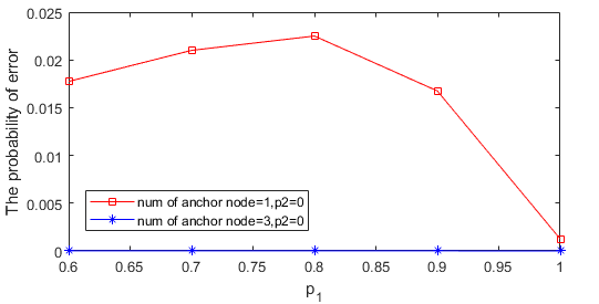
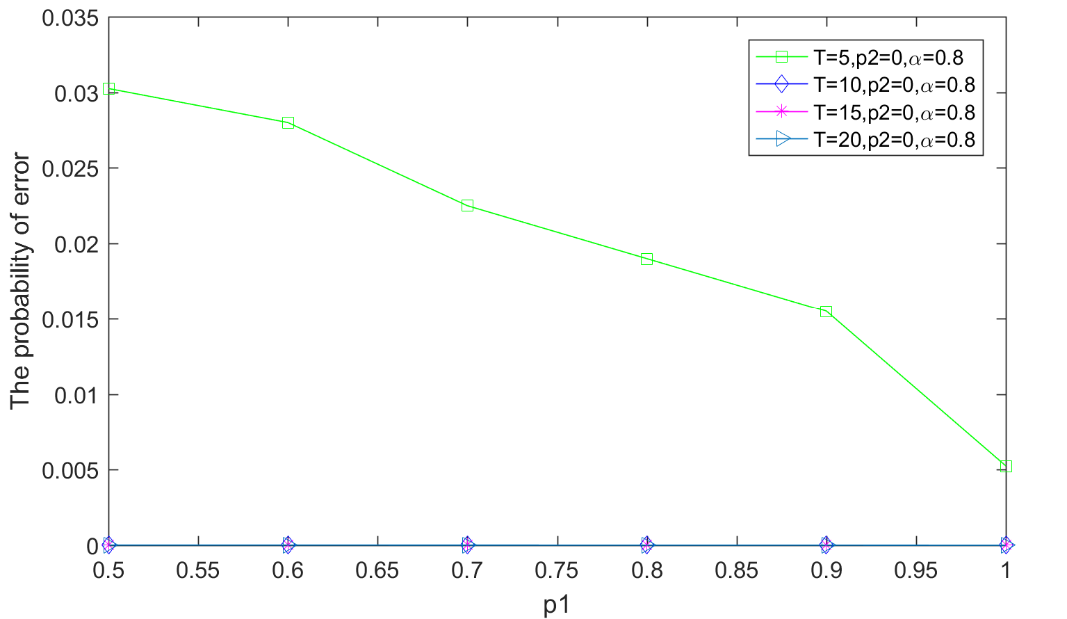
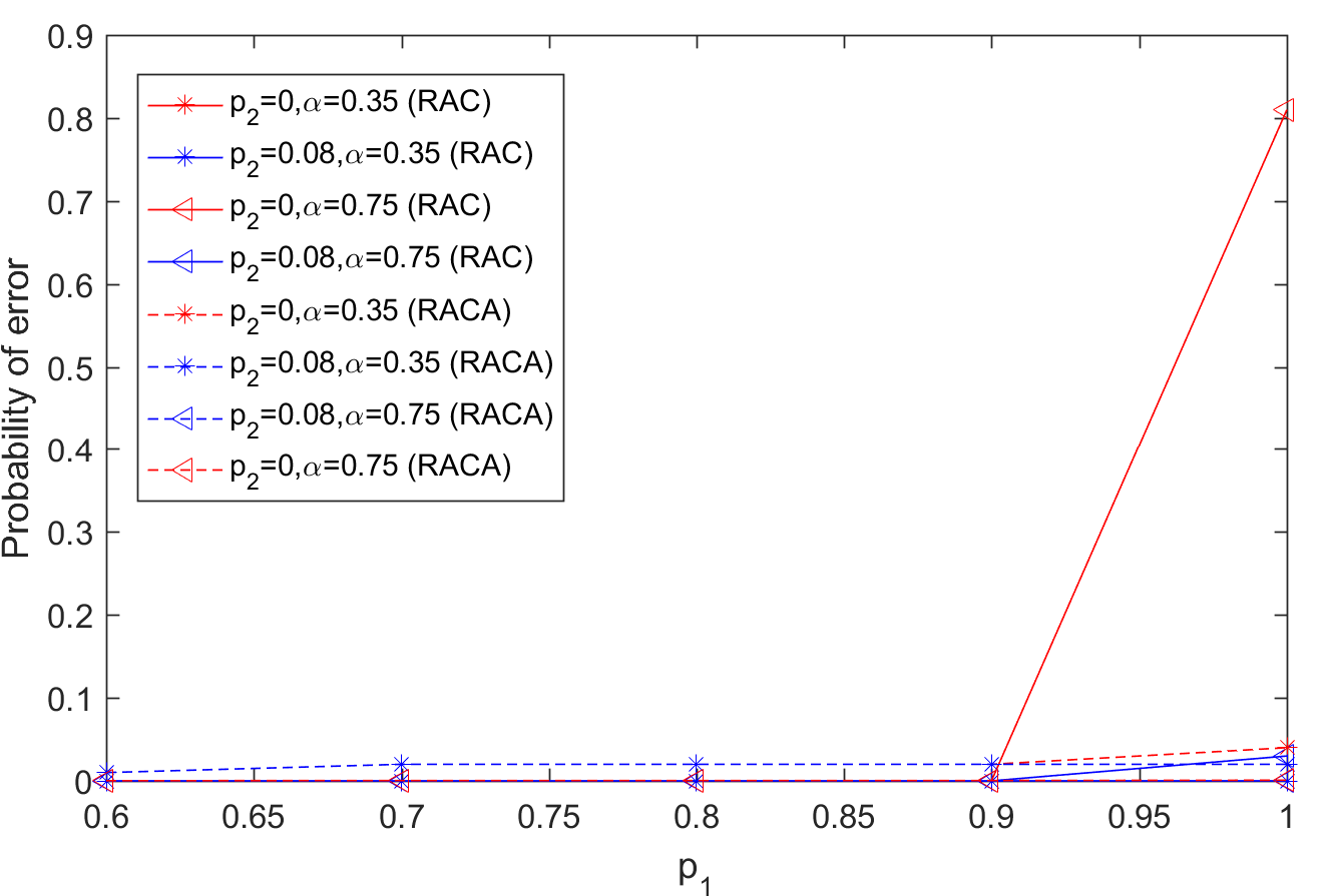
In Fig. 2(a), we can observe that the proposed algorithm with one anchor node (i.e., RACA) and the one without anchor nodes (i.e., RAC) both have outstanding detection performance when the fraction of Byzantine nodes . Fig. 2(b) shows that the system can still obtain a good detection performance with the help of anchor nodes even when the fraction of Byzantine nodes is greater than . It can be observed that the detection performance of the RAC degrades significantly only when approaches 1 and approaches 0 if the fraction of Byzantine nodes is greater than 0.5. We compare our proposed algorithms with other two algorithms in Fig. 2(a). It shows that our proposed algorithms outperform Adaptive reputation clustering algorithm (ARC) proposed in [9] and Reputation based algorithm (RBA) proposed in [7]. Note that those algorithms (ARC and RBA) immediately break down when over half of the sensors are Byzantine nodes. In Fig. 3, we show that our proposed algorithms are able to quickly identify Byzantine nodes so that we can obtain an excellent detection performance. Furthermore, we examined the impact of the number of anchor nodes used on the performance of the system in Fig. 4. It shows that an increasing number of anchor nodes significantly enhances the detection performance of the system since a larger number of anchor nodes could provide the FC better reference decisions to identify the Byzantine nodes. In Fig. 5, we show that at least 10 decision records, i.e., , are needed to guarantee a relatively good detection performance.
Fig. 6 shows the detection performance of our proposed algorithms under Byzantine attacks with dynamically changing attacking parameter . In each time step, we assume that the real value of is uniformly generated from in order to represent the dynamically changing attacking parameter . The average error probability we obtain for a specific dynamically changing is the error probability that corresponds to in Fig. 6. We can observe that our proposed algorithms are able to defend against attackers whose attacking parameters are dynamically changing. It is due to the fact that the performance improvement of our proposed algorithms is directly affected by the deviation of Byzantine nodes’ decision records from those of honest nodes, and the deviation is the reflection of and in the system. Hence, the dynamically changing attacking parameters in each iteration do not result in a significant impact on the ability of our proposed algorithms to defend against attacks.
V CONCLUSION
In this paper, we proposed the RAC algorithm and the RACA algorithm to defend against Byzantine attacks in sensor networks when the FC is not aware of the attacking strategy. We utilized the history of local decisions and MMS results to update the reputation index of sensors and help the system accurately identify Byzantine nodes. Our simulation results showed that we are able to achieve superior detection performance and the enhanced ability of identifying Byzantine nodes by employing anchor nodes even when the Byzantines exceed half of the total number of sensors in the network. Furthermore, we showed that our algorithms are capable of defending against attackers whose attacking parameters change dynamically over time.
Appendix A Proof of Lemma III.1
We have the following four cases when we consider the MMS results of the sensors in the same group. Let and represent the sensors in the same group.
If and
is a Byzantine node with probability
| (11) |
where , and .
If and
is a Byzantine node with probability
| (12) |
where , , and .
If and
is a Byzantine node with probability
| (13) |
where , , and .
If and
is a Byzantine node with probability
| (14) |
where , and .
According to the above results, we have
| (15a) | ||||
| (15b) | ||||
The derivative of with respect to is given by (note that )
| (16) |
where , , and . Let , we have
| (17) |
due to the fact that , where
| (18) | ||||
| (19) |
We can easily obtain that makes the equation (17) always hold for any specific . In other words, we can obtain that could minimize or maximize given a specify . Correspondingly, could also maximize or minimize . Table I shows all the possible maximum or minimum values of given a specific .
According to Table I, we have
| (20) |
for and
| (21) |
for or . Let represent the difference between and , and it is given by
| (22) |
for , and it is given by
| (23) |
for or . Because we only care about the sign of and the numerator is always positive. Let denote the numerator of . We have
| (24) |
We can easily obtained that for and for given . According to (24), We can prove that always holds for . When , also holds for .
When and , the value of that guarantees should be smaller than . can be obtained from letting and it is given by
| (25) |
for and . Note that implies such that . Hence, if the fraction of Byzantine nodes in the network is smaller than 0.8, i.e., , is always smaller than . In other words, we always have a lower probability of existence of Byzantine nodes in set when . The detailed proof for this part is omitted here. Fig. 7 corroborates the results in (25).

References
- [1] L. Zhang, G. Ding, Q. Wu, Y. Zou, Z. Han, and J. Wang, “Byzantine attack and defense in cognitive radio networks: A survey,” IEEE Communications Surveys & Tutorials, vol. 17, no. 3, pp. 1342–1363, 2015.
- [2] L. Lamport, R. Shostak, and M. Pease, “The Byzantine generals problem,” in Concurrency: the Works of Leslie Lamport, 2019, pp. 203–226.
- [3] R. P. Jover, J. Lackey, and A. Raghavan, “Enhancing the security of lte networks against jamming attacks,” EURASIP Journal on Information Security, vol. 2014, no. 1, pp. 1–14, 2014.
- [4] K. Gai, M. Qiu, Z. Ming, H. Zhao, and L. Qiu, “Spoofing-jamming attack strategy using optimal power distributions in wireless smart grid networks,” IEEE Transactions on Smart Grid, vol. 8, no. 5, pp. 2431–2439, 2017.
- [5] J. Sonnek, A. Chandra, and J. Weissman, “Adaptive reputation-based scheduling on unreliable distributed infrastructures,” IEEE Transactions on Parallel and Distributed Systems, vol. 18, no. 11, pp. 1551–1564, 2007.
- [6] K. Zeng, P. Pawelczak, and D. Cabric, “Reputation-based cooperative spectrum sensing with trusted nodes assistance,” IEEE communications letters, vol. 14, no. 3, pp. 226–228, 2010.
- [7] A. S. Rawat, P. Anand, H. Chen, and P. K. Varshney, “Collaborative spectrum sensing in the presence of Byzantine attacks in cognitive radio networks,” IEEE Transactions on Signal Processing, vol. 59, no. 2, pp. 774–786, 2010.
- [8] B. Kailkhura, Y. S. Han, S. Brahma, and P. K. Varshney, “On covert data falsification attacks on distributed detection systems,” in 2013 13th International Symposium on Communications and Information Technologies (ISCIT). IEEE, 2013, pp. 412–417.
- [9] A. Vempaty, P. Ray, and P. K. Varshney, “False discovery rate based distributed detection in the presence of Byzantines,” IEEE Transactions on Aerospace and Electronic Systems, vol. 50, no. 3, pp. 1826–1840, 2014.
- [10] B. Kailkhura, Y. S. Han, S. Brahma, and P. K. Varshney, “Distributed Bayesian detection in the presence of Byzantine data,” IEEE transactions on signal processing, vol. 63, no. 19, pp. 5250–5263, 2015.
- [11] W. Hashlamoun, S. Brahma, and P. K. Varshney, “Mitigation of Byzantine attacks on distributed detection systems using audit bits,” IEEE Transactions on Signal and Information Processing over Networks, vol. 4, no. 1, pp. 18–32, 2017.
- [12] ——, “Audit bit based distributed Bayesian detection in the presence of Byzantines,” IEEE Transactions on Signal and Information Processing over Networks, vol. 4, no. 4, pp. 643–655, 2018.
- [13] C. Quan, B. Geng, Y. Han, and P. K. Varshney, “Enhanced audit bit based distributed Bayesian detection in the presence of strategic attacks,” IEEE Transactions on Signal and Information Processing over Networks, 2022.
- [14] L. Kaufman and P. J. Rousseeuw, Finding groups in data: an introduction to cluster analysis. John Wiley & Sons, 2009, vol. 344.
- [15] B. Kailkhura, S. Brahma, and P. Varshney, “On the performance analysis of data fusion schemes with Byzantines,” in 2014 IEEE International Conference on Acoustics, Speech and Signal Processing (ICASSP). IEEE, 2014, pp. 7411–7415.