Hierarchical Embedded Bayesian Additive Regression TreesPublication type: Article Type
Abstract
We propose a simple yet powerful extension of Bayesian Additive Regression Trees which we name Hierarchical Embedded BART (HEBART). The model allows for random effects to be included at the terminal node level of a set of regression trees, making HEBART a non-parametric alternative to mixed effects models which avoids the need for the user to specify the structure of the random effects in the model, whilst maintaining the prediction and uncertainty calibration properties of standard BART. Using simulated and real-world examples, we demonstrate that this new extension yields superior predictions for some of the standard mixed effects models’ example data sets, and yet still provides consistent estimates of the random effect variances. We illustrate the new tool with example data sets from widely-used mixed effects model packages.
keywords
Bayesian Additive Regression Trees, hierarchical models, hierarchical trees, mixed modelsInitialize: \algnewcommand\Init
Wundervald et al.
Maynooth, Kildare, Ireland.
1 Introduction
Bayesian Additive Regression Trees (Chipman \BOthers. \APACyear2010, BART;) is a commonly-used probabilistic machine learning approach that produces predictions based on sums of regression trees. Like most standard machine learning approaches, however, BART is not mathematically designed to deal with hierarchical structures in the data. For example, certain observations may share common grouping characteristics e.g. repeated measures and grouped data (Gelman \BBA Hill \APACyear2006), where there is an intra-group variance that needs to be accounted for when fitting the model. There are, of course, some algorithm options that can fit statistical methods to grouped data (Bates \BOthers. \APACyear2011, e.g.), but they are often not flexible or able to adapt to data that has been generated by a complicated underlying structure. It might also happen that certain observations have their grouping information missing (Vallejo \BOthers. \APACyear2011), or predictions might be required at different levels of the data hierarchy, which leads to even more complicated scenarios. Occasionally it is of interest to estimate and/or remove the variability associated with the structured component of the data. The user is often left with a difficult model selection task, as they must choose whether the random effects go into an intercept or a slope or an interaction. Due to the complexity of this task, the model space is not usually well-explored. Literature has arisen on the need to explore and check hierarchical models (Gelman \BBA Hill \APACyear2006, see e.g. Chapter 24 of).
With this in mind, Hierarchical Embedded BART (HEBART) introduces a hierarchical component in order to properly model grouped data and estimate the manner through which the hierarchical component of the data enters into the predictions using Bayesian Additive Regression Trees. This is substantially different to the original means by which random effects have been proposed as an inclusion to the BART model; see Section 7 of Chipman \BOthers. \APACyear2010. By contrast, in the simplest version of our model, the hierarchical component is a single categorical predictor variable that adjusts all the predictions in the terminal nodes of each tree. Thus the effects are no longer confined to individual components of the model (e.g. intercept terms) and so, give much greater flexibility whilst still providing the predictions at multiple layers of the hierarchy. Moreover, we do not make it a requirement for the grouping information to exist when calculating the predictions, which allows us to predict for observations where the group is missing, or when the variability associated with the grouping information should be removed, bringing even more flexibility to our approach. We provide full technical details of our extension below.
Our paper is structured as follows. In Section 2 we introduce the BART model mathematically, and discuss the fitting algorithm and some extensions that have already been proposed. In Section 3 we outline our new HEBART approach and discuss how this extends BART into a generalized model for hierarchical data structures, whilst retaining the attractive properties and algorithmic efficiency that BART exhibits. In Section 4 we demonstrate the performance of the method on simulated and real-world data. Finally, Section 5 discusses some of the potential future research areas and drawbacks of our approach. An appendix contains some of the more detailed mathematics behind the fitting algorithm.
2 Introduction to Bayesian Additive Regression Trees
2.1 The BART model
The initial Bayesian Regression Tree model was first proposed over 20 years ago (Chipman \BOthers. \APACyear1998), and consists of an algorithm that fits CART decision trees using Bayesian inference. The same authors extended this method to create the Bayesian Additive Regression Tree (Chipman \BOthers. \APACyear2010) approach, which assumes that the generating system of a continuous random variable can be approximated by a sum of regression trees. In a standard regression setting the BART model is usually written as:
| (1) |
for observations , and trees with the total (fixed) number of trees, represents the set of covariates; is a tree structure, and represents a set of terminal node parameters. The function returns a terminal node prediction from by passing through the tree . consists of a set of parameters for each of the terminal nodes in tree . These values provide the tree-level predictions which are summed together to give an overall predicted value. The residual term is assumed normal with residual precision . Figure 1 (left panel) shows a standard single tree that a BART model may use.
We write the set of all trees and parameters as and respectively. The joint posterior distribution of the trees and all the parameters is then given by:
| (2) |
where is the normally distributed likelihood as defined in Equation 1, represents the regions in the covariates space (e.g. tree nodes), and indexes the terminal nodes in tree . The term is the prior distribution on the terminal node parameters across each terminal node in each tree . is the prior distribution on the tree structure, and is the prior on the residual precision. We detail all these terms below.
The prior distribution on the trees proposed by Chipman \BOthers. \APACyear2010 involves applying a separate term for each node in the tree and considering both the probability of a split as well as the probability of a new splitting variable being chosen. For an entire tree , we have:
where and represent the sets of terminal and internal nodes, respectively, represents a generic splitting value, and represents a node in the tree. The probability of a node being non-terminal is given by , where denotes the depth of the node . The recommended values for the hyperparameters are and , which control the depth and bushiness of the trees. For the probability of the new splits, where represents how many predictors are still available to split on in node , and how many values in a given predictor are still available.
The prior distribution for the terminal node and overall parameters in the standard regression case is denoted by . This is given a prior with a standard conjugate form:
where and are chosen such that a high density of this distribution is apportioned to the range interval, by setting and , for some value of . The response is usually standardized before the model is run which allows for reasonable guesses as to the hyper-parameter values of and , though these too can be estimable parameters.
The residual precision prior is set as where and are fixed. An oft-used tactic is to set the two hyper-parameters such that the BART residual precision is greater than an equivalent precision value from a standard linear regression model applied to the same data with a high probability. We follow the same guidance in our extension to the model as outlined below.
Since its creation, BART has been applied in a wide variety of different application areas. The model has been shown to be useful for credit risk modeling (Zhang \BBA Härdle \APACyear2010), survival data analysis (R\BPBIA. Sparapani \BOthers. \APACyear2016; R. Sparapani \BOthers. \APACyear2020), ecology and evolution modelling (Carlson \APACyear2020), weather and avalanche forecasting (Blattenberger \BBA Fowles \APACyear2014), and genetics (Waldmann \APACyear2016). A popular approach is its use in causal inference (Hill \APACyear2011; Hahn \BOthers. \APACyear2020), where BART produces accurate estimates of average treatment effects and is competitive even with the true data generating model.
Beyond applications, many fundamental extensions to the standard BART model have been proposed. Some of the first include adapting BART for categorical, count, and multinomial regression (Murray \APACyear2017; Kindo, Wang\BCBL \BBA Peña \APACyear2016) and quantile regression (Kindo, Wang, Hanson\BCBL \BBA Pena \APACyear2016). This was followed by the proposal of BART that adapts to smoothness and sparsity (Linero \BBA Yang \APACyear2018\APACexlab\BCnt1), models for high-dimensional data and variable selection (Linero \APACyear2018\APACexlab\BCnt1), BART for zero-inflated and semi-continuous responses (Linero \BOthers. \APACyear2020) and an extension proposed by (Hernández \BOthers. \APACyear2018), where the authors combine BART with Bayesian Model Averaging to obtain posterior distribution more efficiently when there is a large number of variables available. More recently BART has been extended for use with heterocedastic data (Pratola \BOthers. \APACyear2020), for the estimation of monotone and smooth surfaces, (Starling \BOthers. \APACyear2020), varying coefficient models (Deshpande \BOthers. \APACyear2020), semiparametric BART (Prado, Parnell\BCBL \BOthers. \APACyear2021), and a combination of BART with model-trees (Prado, Moral\BCBL \BBA Parnell \APACyear2021). As this is a fairly new class of machine learning algorithm, progress on the theoretical performance of BART has only just begun. Some of the mathematical properties of BART, including a deep review of the BART methodology can be found in Linero \APACyear2017, and some more general theoretical results in Ročková \BBA van der Pas \APACyear2020; Ročková \BBA Saha \APACyear2019.
2.2 Fitting algorithm
The BART model is fitted via a backfitting MCMC algorithm (Hastie \BBA Tibshirani \APACyear2000) that holds all other trees constant while the current one is being updated. This involves calculating the full conditional distribution , where represents the set of all trees except for tree (the definition of is analogous). This conditional depends on only via the current state of the residuals, defined as
meaning these partial residuals include the sum of the predictions for all trees except . The choice of prior distributions on the trees and terminal nodes allows for the term to be calculated in closed form which avoids the need to trans-dimensional MCMC methods, and greatly simplifies the resulting algorithm.
The algorithm samples from via two main steps:
- 1.
propose a new tree through one of 4 proposal moves and calculate , and
- 2.
sample a new set of terminal node parameters via , for the new tree
The new trees are proposed using a Metropolis-Hastings sampler (Brooks \BOthers. \APACyear2011), where the candidate tree is obtained via: GROW (a terminal node is selected uniformly from the set of terminal nodes and split into two, with a new split variable and split value chosen analogously), PRUNE (a pair of terminal nodes with a common parent are collapsed together), CHANGE (a splitting rule is chosen uniformly across the tree and is changed to a new split variable and split value) or SWAP (a parent-child pair of internal nodes is chosen uniformly and swapped in the tree). The movement choice requires probabilities for each move, which can be equal or depend on prior beliefs about moves that should be prioritized. The means by which the splitting variable and value are chosen are slightly different across the implementations of BART in the literature. Pratola \APACyear2016 propose even more detailed moves for the generation of new candidate trees, and (Linero \APACyear2018\APACexlab\BCnt2) puts a Dirichlet hyperprior on the splitting rules, such that the algorithm keeps track of which variables are most useful for splits and avoid using too many variables.
3 Hierarchical Embedded Bayesian Additive Regression Trees (HEBART)
Our HEBART approach merges the ideas from traditional Bayesian hierarchical modeling (Gelman \BBA Hill \APACyear2006) and linear mixed effects models (Pinheiro \BBA Bates \APACyear2000) with BART. We allow each tree to have an extra split on each terminal node corresponding, in the simplest version, to a random intercept for each member of a categorical predictor variable which takes values according to the group membership of observation . Thus we introduce intra-group node parameters which we write as as the estimate for group in terminal node . We refer to these parameters as the sub-terminal node level. Here, the term ‘embedded’ is used to represent the inclusion of the grouping variable into the BART model at the terminal node level rather than as a simple addition on the BART mean, as was originally proposed as an extension to BART in Chipman \BOthers. \APACyear2010. The new parameters allow us to have a group-specific prediction for each node, as well as an overall terminal node prediction . The flexibility of this structure means that there is no requirement for the user to specify where the random effect is included, for example as an intercept or as a regression slope. With HEBART we can fit Bayesian Additive Regression Trees to any kind of grouped data where there is such a categorical predictor, such as longitudinal data, repeated measures data, multilevel data, and block designs. In addition, having the two levels of predictions is advantageous for scenarios where the group information is not available for all or a subset of the new data. The Bayesian paradigm allows for imputation of any missing groups at any of the terminal nodes. In Figure 1 we show a standard BART tree alongside that of our new HEBART trees.

To define the HEBART model, let be the number of trees, to be the total number of groups, and the set of node parameters at both the terminal node and sub-terminal node level. More fully, we have one set which are terminal node predictions for each tree, and one set for each group within each sub-terminal node for tree , . Assuming we have a continuous variable of interest, the fundamental HEBART appears similar to the standard BART approach:
| (3) |
for observation with grouping variable taking values from to . In this specification, we have that is the tree look-up function which allows for predictions based on covariates and categorical grouping values ; by default will return a sub-terminal node prediction value . If the grouping variable is not provided it will return a terminal node estimate , which we may write as for clarity. In other words, is the function that maps each estimated tree structure to the corresponding values of the covariates and finds in which terminal node of the tree each observation falls into (see, e.g, Figure 1, right panel, for an example). With this, the function uses the tree structures to attribute the correct predicted value for each observation. Similar to an LME model, the parameters associated with the categorical grouping variable provide shifts away from the overall means and are constrained using a normally distributed prior. As before is the tree structure, but now contains both the terminal node parameters () and the sub-terminal node group parameters () for tree . As with standard BART, the noise is assumed to be distributed as , where is the overall residual precision.
The and sets contain, respectively, the overall terminal-node mean parameters and the intra-group sub-terminal node mean parameters. In other words, for each tree we will have one set for each of their terminal nodes, and for each group within each terminal node we will have another set . All parameters in receive priors and have their corresponding posteriors, from which we sample from in the fitting algorithm. In Figure 1 the terminal circles represent the terminal nodes, which all have their own parameters. In the HEBART tree, however, we have the addition of the intra-group parameters, represented by the hexagonal symbols at the sub-terminal node level.
In standard BART a minimum node size is usually set on the number of data points that fall into each terminal node. We retain that restriction in our approach but require no such restriction for the sub-terminal node levels. As shown below, the Gibbs update for the terms is still available even when no residuals fall into that particular group so we can still provide group-level predictions which can be summed over trees to produce group-level predictions from every tree.
3.1 Prior distributions
Many of the standard BART prior distributions carry over to our situation, which desirably means that certain parametric restrictions in our model will yield an exact BART model. Specifically, we have as usual for the terminal nodes (ignoring node index subscripts for simplicity). As in standard BART, we standardize so that and is simple to calibrate using the heuristics outlined above. We have for the residual precision. We keep the tree prior and its hyper-parameters to control the shape and structure of trees. For the sub-terminal node parameters, we simply set which forces each sub-terminal node to vary according to around the terminal node parameter, scaled by the number of trees. Unlike we treat as a parameter to be estimated, and provide more details of this below.
For HEBART, a single sub-terminal node in tree has partial residuals:
| (4) |
for observation with cateogorical variable . Now, let represent the full set of residuals for those observations where , where we drop the dependence on terminal node and tree for simplicity of notation, and vectorize it again so we can write . In this fashion, represents all observations in that particular terminal node for that particular tree now across all groups, is a binary matrix that allocates observations in the terminal node to groups, and represents the stacked vector of terminal node parameters for all groups in that terminal node. Marginalising first over and then over , we obtain a distribution on the partial residuals as , where . This variance matrix is symmetric and can be inverted quickly when required using Woodbury and related formulae.
We give the parameter, responsible for capturing the intra-group precision, a prior. Since the value of is analogous to that of a standard LME model we first fit a random intercept model to the same data using the lme4 package (Bates \BOthers. \APACyear2014) and write this estimated precision as . We further extract the variance of this estimate via the parameters package (Lüdecke \BOthers. \APACyear2020) which we write as . The given mean and variance then provide simple point estimates of and using the standard method of moments, where we find those values such that . Our approach is analogous to the argument used in standard BART to set via the residual variance of a linear model fit, though there the BART residual variance is expected to fall below the linear model fit with high probability. To set our prior for , we calibrate the hyper-parameter values using the same rule as BART, but via the residual variance of the above lme4 model fit rather than the standard linear model. In this case, our strategy aims to yield a high probability that is bigger than , so we find prior hyperparameters such that .
3.2 Links with standard hierarchical models
Conditional on the trees, the model can be written as a standard linear mixed effects model. We abuse the above notation slightly to write:
| (5) |
where is the vector of all observations and is a binary matrix that allocates each observation to its correct tree and sub-terminal node. The number of columns of can be large when the number of trees and/or terminal nodes is large, and changes dimension when the conditioning on the trees is removed. here is the stacked vector of all sub-terminal node parameters sorted over all trees. This parameter too can be marginalized over since, within each tree, all components come from a distribution. This second marginalization yields:
| (6) |
where now is the stacked terminal node values across all trees and . is a binary allocation matrix that allocates each observation to the terminal nodes associated with its trees. With this second marginalization there are several links with standard Bayesian mixed effects models frameworks. The model can be seen as a Gaussian Process with kernel autocorrelation function given by , or as a standard mixed effects model with with a prior on centered on zero. The standard theory of LMEs (Pinheiro \BBA Bates \APACyear2000, e.g.) follows directly, and in the Bayesian framework, the updates for sub-terminal node parameters yields the usual partial pooling estimates exemplified by Gelman \BBA Hill \APACyear2006; see updates for below. However, the mixing over the trees makes any further theory considerably more complex, and we leave this as a challenge for future research.
3.3 Updating parameters
We use MCMC methods to update the parameters, using direct Gibbs sampling for updating the terminal node and residual precision parameters, and Metropolis updates for those for which a tractable Gibbs update is unavailable. The updates for an individual tree arise by considering the distribution of the partial residuals in a single terminal node, whilst integrating out the mean and variance parameters. We use the marginalized version of above to find an MH update for a single terminal node in a tree (on the log scale, and summed over terminal nodes ) as:
For , we use the non-marginalised prior for and the prior on to obtain the full conditional:
which is used to directly sampled values for the parameters. In this equation, we have that . Similarly, we also obtain a closed-form posterior distribution for :
After all trees are updated we can update . The update comes directly from the non-marginalised prior for combined with the prior on :
Last, we use a random-walk Metropolis-Hastings update for , which we found to be reliable for sampling from this posterior (Brooks \BOthers. \APACyear2011). We use a standard Normal for the proposal value to create and decide to accept or reject it based on the acceptance probability , where represents the CDF of the standard Normal distribution. This is used to account for the fact that we are using a proposal distribution with full support for a target with limited support.
[ht] HEBART Algorithm
Type: Metropolis within GIBBS for a hierarchical BART model
y, X, grouping variable \EnsurePosterior distribution of trees , , , and \InitInitial values for , , , , number of trees P, stumps , number of observations N, number of MCMC iterations , initial residual set \For to \For to P
- 1.
Grow a new tree tree by either growing, pruning, changing or swapping a root node
- 2.
Calculate
- 3.
Sample
- 4.
if then do
to : Sample \For to : sample \EndFor\EndFor\StateUpdate
Update
Sample \StateSample : \State Sample a value and make \State Calculate \State Sample \Stateif then do
4 Applications & Results
This section describes the fitting of HEBART to some example data sets as we compare across different models, including: a Linear Mixed-Effects (LME) model, fitted using the lme4 (Bates \BOthers. \APACyear2011) package; in R (R Core Team \APACyear2020) and standard BART, fitted using the dbarts (Dorie \APACyear2021) R package, with the default values for the number of trees (200), number of posterior samples (1000), number of burn-in samples (100). The main performance results presented are calculated on out-of-sample values for a certain number of test sets. Since BART cannot incorporate mixed effects, other than as part of the main covariate set, we partition the results into BART including grouping information, which we expect to perform well though it does not solve the hierarchical modeling problem, versus BART without grouping information, which usually performs worse than our approach since it lacks all the data.
The package created to run our HEBART algorithm is available in R (R Core Team \APACyear2020). All functions are available at https://github.com/brunaw/hebartBase, where the main package is stored, and https://github.com/brunaw/hebart-experiments contains the code for replicating all the examples shown here, with their corresponding auxiliary files.
4.1 Simulation experiments
We first experiment with HEBART on a simple simulation scenario, where the response variable is simulated as a sum of a tree structure and an intra-group parameter, which here we call and are simulated from a to create highly variant values. By splitting the simulated covariates at random points, we sample values as
| (7) |
where we have for all 5 groups and are randomly sampled from a . This experiment uses 10 different train and test sets as our cross-validation setting (Refaeilzadeh \BOthers. \APACyear2009).
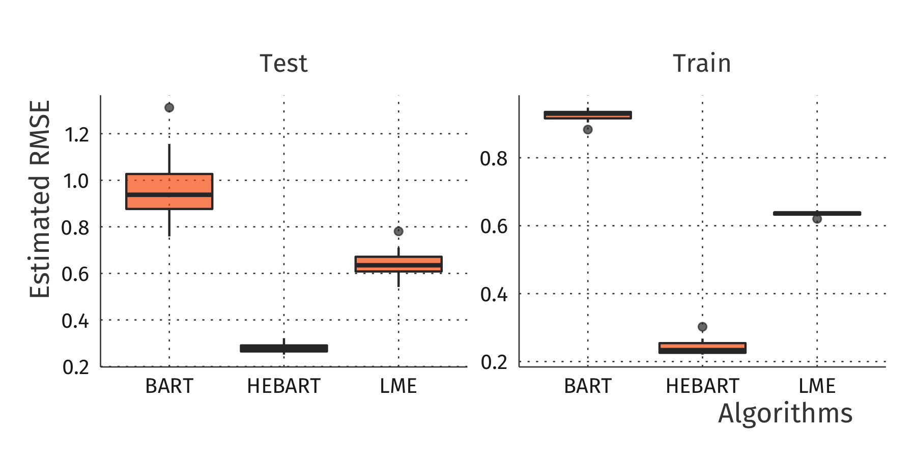
To these simulated datasets, we apply three different algorithms (LME, Standard BART and HEBART) to the 10 training sets and make predictions for the 10 testing sets. In Figure 2, we can see that HEBART produces the smallest root mean squared errors for both the train and test sets, as its averages are the closest to zero, followed by LME and standard BART. We also observe that HEBART has the least varying RMSE values on the test set, implying there is less uncertainty around the predictions for new data.
In a second simulation setting we create with a direct HEBART structure, by first sampling a value for each terminal node, along with one value for each group within the created terminal nodes, where and . The tree structure uses the sum of two simple trees, which are both based on two covariates , and uses the previously sampled parameters to create the simulated response . By splitting the simulated covariates at random points, we sample values as
| (8) |
where . Tree consists of three terminal nodes with the partitions , , respectively, having terminal node values sampled from a , and group terminal node values sampled from a , , as we have 3 terminal nodes. For tree the partitions are only and , having terminal node values sampled from a , and and group terminal node values sampled from a , .
The results of this simulation are shown in Figure 3. Once again, we observe HEBART to be the best-performing algorithm, as its test RMSE average is lower than its competitors. We also include here the prior and posterior densities of one of the runs of the HEBART model. The two densities are markedly different, with the posterior having a distinctly larger variance (lower precision) associated with the grouping information. This is not necessarily surprising given that the grouping information for this simulation scenario is specified at the sub-terminal node level rather than through an additive effect as is used in an LME.
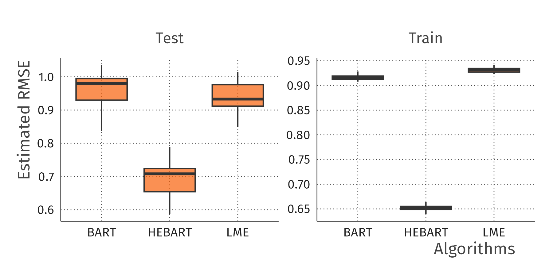 |
| (a) Boxplots of RMSE for testing and training sets for the 3 algorithms fitted on simulated data |
 |
| (b) Prior and posterior densities for for one run of HEBART |
4.2 Real data sets
4.2.1 Sleep study data
This dataset consists of the first 10 days of a sleep study (Belenky \BOthers. \APACyear2003). The response variable is the average reaction time per day (in milliseconds), and the covariate is the number of days of sleep deprivation, for 18 subjects. Linear mixed-effect models (Pinheiro \BBA Bates \APACyear2000) are often applied to this data (Bates \BOthers. \APACyear2011), so we can directly compare our results.
We create a 20-fold cross-validation and evaluate the model on the left-out data. Our HEBART model is set to use 10 trees, has hyperparameters = 0.95 and = 2, and all the other prior hyperparameters are set as described above. For the MCMC sampling, we use 1500 iterations with 250 iterations of burn-in. We also fit an LME (Pinheiro \BBA Bates \APACyear2000) and a standard BART model (Chipman \BOthers. \APACyear2010) to compare our results. Our main interest is in the performance of the predictions and the estimate of the group-level random effect standard error, though this is not available in the BART model since it has no such parameter. However, as described above the grouping variable is sub-optimally included as one of the covariates.
In Figure 4 we show the HEBART, BART and LME predictions for each group ID, for predictions created when those observations were not included in the training set. In other words, we are seeing the average predictions for the test sets, split by group ID. The plot also shows the true observations as green dots for comparison. We can see for almost all IDs, the HEBART predictions are the ones closest to the true values, especially for more difficult cases, such as IDs 335, 332, 351 and 351. Overall, HEBART is able to adapt better to changes in each of the individual group patterns. In the same Figure, we also have the RMSE table for each model, with their corresponding empirical 95% confidence intervals, calculated using the results from the 20 train and test sets. From this table it is clear that HEBART produces the best results, as both the train and test RMSEs are the lowest of the three methods, with similarly low values for the confidence intervals.
 |
| (a) Average predictions for the groups in the sleep study dataset |
| Source | HEBART | LME | BART+Group |
|---|---|---|---|
| Test set | 27.7 [8.22, 47.2] | 32.4 [15.8,49] | 32.3 [13.3, 51.2] |
| Train set | 16.9 [10.1,23.7] | 29.3 [28.3,30.3] | 28.1 [26.6,29.6] |
| (b) Average train and test set RMSE values, with the corresponding empirical 95% confidence intervals |
4.2.2 Gapminder data
Another standard dataset used to exemplify mixed effects modeling is the Gapminder data (Lang \APACyear2011). For our experiment, the subset of the data consists of the life expectancy values (in years) for 20 different countries, from 1950 to 2018. We use life expectancy as the response and country as the grouping variable with year as the sole covariate. We separate the dataset into 10 different training and test sets, where the testing set is composed of all the observations for 15 sampled years (for all countries), and the corresponding training set is composed of the observations for the remaining data. The idea behind this is, for each resample, to fully remove a set of years from the training set to make it harder for the model to predict for such years, since it has no information about what happened in the removed years. We also compare our model against LME, BART and BART using the country as a covariate. We expect the latter to perform well since it has all the information, but we remind the reader that this method does not have the added advantage of HEBART in being able to predict with fully or partially missing grouping values.
Figure 5 shows the results for this experiment as an RMSE table and the depiction of the predicted values in comparison to the true observations. Note that we have 10 training and test sets, and what we show in the Figure are the average predictions for the 10 test sets. So, when we bind all the predictions for all the 10 test sets, we have at least one prediction for each year of all countries. As above, the HEBART prediction is very close to the actual values due to the increase in flexibility of the predictions from the non-parametric structure. The performance of the BART model that uses the country as a covariate (BART+Group) is slightly superior but as stated above, this is not unexpected since the BART+Group misses the fundamental advantage of HEBART in separating out (and potentially removing) the country-level variability. Our model, on the other hand has the advantage of being able to predict when grouping variable information is missing, but still retains the prediction performance.
 |
| (a) Average out of sample predictions for selected countries in the gapminder dataset |
| Source | HEBART | LME | BART | BART+Group |
|---|---|---|---|---|
| Test set | 1.33 [0.77, 1.88] | 3.59 [2.84, 4.33] | 7.53 [6.53, 8.52] | 0.815 [0.43, 1.20] |
| Train set | 0.793 [0.162, 1.42] | 3.57 [3.38 , 3.77] | 7.47 [7.20, 7.73] | 0.351 [0.310, 0.391] |
| (b) Average training and test RMSE values, with the corresponding empirical 95% confidence intervals |
5 Conclusions
We have provided a new extension of Bayesian Additive Regression Trees that allows for structured data to be used appropriately at the model fitting and prediction stage. Where a grouping variable is present, we are able to provide predictions at both the group level and the level above it. The flexible tree structure thus allows us to produce excellent predictions without the need to specify how the grouping variable is included in the model structure. However, we still retain the ability to report and remove the group-level variability by having a parameter that represents the group-level standard deviation.
In simulation-based and real data studies we have shown that the model performs better than other common linear and mixed effects approaches or BART itself. Our approach is not comparable to many other standard Bayesian machine learning methods due to their inability to handle the grouping information other than as a naïve covariate. In the real data examples of Section 4.2.1 and 4.2.2 we have demonstrated that HEBART performs well against LME modelling strategies despite these being the archetypal examples of datasets where linear mixed-effects models would fit well. Finally, We see many potential extensions of our approach, including: (1) extending the hierarchical data structure to multiple or nested grouping variables; (2) explicitly modeling joint random effects using the multivariate normal distribution and so estimating covariances between grouping variables; (3) including recent BART extensions, such as SOFT-BART (Linero \APACyear2018\APACexlab\BCnt1) and MOTR-BART (Prado, Moral\BCBL \BBA Parnell \APACyear2021) which can substantially enhance the predictive capabilities of the model;
Acknowledgments
00footnotetext: Abbreviations: BART, Bayesian Additive Regression Trees; HEBART, Hierarchical Embedded Bayesian Additive Regression Trees; MH, Metropolis-Hastings; MCMC, Monte Carlo Markov Chain; RMSE, Root Mean Squared Error; LME, Linear Mixed-Effects;Acknowledgments
This work was supported by the Science Foundation Ireland Career Development Award grant number: 17/CDA/4695. Andrew Parnell’s work was also supported by: a Science Foundation Ireland investigator award (16/IA/4520); a Marine Research Programme funded by the Irish Government, co-financed by the European Regional Development Fund (Grant-Aid Agreement No. PBA/CC/18/01); European Union’s Horizon 2020 research and innovation programme InnoVar under grant agreement No 818144; SFI Centre for Research Training in Foundations of Data Science 18/CRT/6049, and SFI Research Centre awards I-Form 16/RC/3872 and Insight 12/RC/2289_P2. For the purpose of Open Access, the author has applied a CC BY public copyright licence to any Author Accepted Manuscript version arising from this submission.
Author contributions
Bruna Wundervald has contributed to the project ideation, mathematical development, code implementation, production and evaluation of results. Andrew Parnell has contributed to the project ideation, mathematical development, code implementation, and evaluation of results. Katarina Domijan has contributed to the project ideation, mathematical development, and evaluation of results.
Financial disclosure
This work was supported by the Science Foundation Ireland Career Development Award grant number: 17/CDA/4695.
Conflict of interest
The authors declare no potential conflict of interest.
References
- Bates \BOthers. (\APACyear2014) \APACinsertmetastarbates2014fitting{APACrefauthors}Bates, D., Mächler, M., Bolker, B.\BCBL \BBA Walker, S. \APACrefYearMonthDay2014. \BBOQ\APACrefatitleFitting linear mixed-effects models using lme4 Fitting linear mixed-effects models using lme4.\BBCQ \APACjournalVolNumPagesarXiv preprint arXiv:1406.5823. \PrintBackRefs\CurrentBib
- Bates \BOthers. (\APACyear2011) \APACinsertmetastarbates2011package{APACrefauthors}Bates, D., Maechler, M., Bolker, B., Walker, S., Christensen, R\BPBIH\BPBIB., Singmann, H.\BDBLGrothendieck, G. \APACrefYearMonthDay2011. \BBOQ\APACrefatitlePackage ‘lme4’ Package ‘lme4’.\BBCQ \APACjournalVolNumPagesLinear mixed-effects models using S4 classes. R package version16. \PrintBackRefs\CurrentBib
- Belenky \BOthers. (\APACyear2003) \APACinsertmetastarbelenky2003patterns{APACrefauthors}Belenky, G., Wesensten, N\BPBIJ., Thorne, D\BPBIR., Thomas, M\BPBIL., Sing, H\BPBIC., Redmond, D\BPBIP.\BDBLBalkin, T\BPBIJ. \APACrefYearMonthDay2003. \BBOQ\APACrefatitlePatterns of performance degradation and restoration during sleep restriction and subsequent recovery: A sleep dose-response study Patterns of performance degradation and restoration during sleep restriction and subsequent recovery: A sleep dose-response study.\BBCQ \APACjournalVolNumPagesJournal of sleep research1211–12. \PrintBackRefs\CurrentBib
- Blattenberger \BBA Fowles (\APACyear2014) \APACinsertmetastarblattenberger2014avalanche{APACrefauthors}Blattenberger, G.\BCBT \BBA Fowles, R. \APACrefYearMonthDay2014. \BBOQ\APACrefatitleAvalanche forecasting: Using bayesian additive regression trees (BART) Avalanche forecasting: Using bayesian additive regression trees (bart).\BBCQ \BIn \APACrefbtitleDemand for Communications Services–Insights and Perspectives Demand for communications services–insights and perspectives (\BPGS 211–227). \APACaddressPublisherSpringer. \PrintBackRefs\CurrentBib
- Brooks \BOthers. (\APACyear2011) \APACinsertmetastarbrooks2011handbook{APACrefauthors}Brooks, S., Gelman, A., Jones, G.\BCBL \BBA Meng, X\BHBIL. \APACrefYear2011. \APACrefbtitleHandbook of markov chain monte carlo Handbook of markov chain monte carlo. \APACaddressPublisherCRC press. \PrintBackRefs\CurrentBib
- Bürkner (\APACyear2017) \APACinsertmetastarburkner2017brms{APACrefauthors}Bürkner, P\BHBIC. \APACrefYearMonthDay2017. \BBOQ\APACrefatitlebrms: An R package for Bayesian multilevel models using Stan brms: An r package for bayesian multilevel models using stan.\BBCQ \APACjournalVolNumPagesJournal of statistical software801–28. \PrintBackRefs\CurrentBib
- Carlson (\APACyear2020) \APACinsertmetastarcarlson2020embarcadero{APACrefauthors}Carlson, C\BPBIJ. \APACrefYearMonthDay2020. \BBOQ\APACrefatitleembarcadero: Species distribution modelling with Bayesian additive regression trees in r embarcadero: Species distribution modelling with bayesian additive regression trees in r.\BBCQ \APACjournalVolNumPagesMethods in Ecology and Evolution117850–858. \PrintBackRefs\CurrentBib
- Chib \BBA Greenberg (\APACyear1995) \APACinsertmetastarchib1995understanding{APACrefauthors}Chib, S.\BCBT \BBA Greenberg, E. \APACrefYearMonthDay1995. \BBOQ\APACrefatitleUnderstanding the metropolis-hastings algorithm Understanding the metropolis-hastings algorithm.\BBCQ \APACjournalVolNumPagesThe american statistician494327–335. \PrintBackRefs\CurrentBib
- Chipman \BOthers. (\APACyear1998) \APACinsertmetastarchipman1998bayesian{APACrefauthors}Chipman, H\BPBIA., George, E\BPBII.\BCBL \BBA McCulloch, R\BPBIE. \APACrefYearMonthDay1998. \BBOQ\APACrefatitleBayesian CART model search Bayesian cart model search.\BBCQ \APACjournalVolNumPagesJournal of the American Statistical Association93443935–948. \PrintBackRefs\CurrentBib
- Chipman \BOthers. (\APACyear2010) \APACinsertmetastarchipman2010bart{APACrefauthors}Chipman, H\BPBIA., George, E\BPBII.\BCBL \BBA McCulloch, R\BPBIE. \APACrefYearMonthDay2010. \BBOQ\APACrefatitleBART: Bayesian additive regression trees Bart: Bayesian additive regression trees.\BBCQ \APACjournalVolNumPagesThe Annals of Applied Statistics41266–298. \PrintBackRefs\CurrentBib
- Deshpande \BOthers. (\APACyear2020) \APACinsertmetastardeshpande2020vcbart{APACrefauthors}Deshpande, S\BPBIK., Bai, R., Balocchi, C., Starling, J\BPBIE.\BCBL \BBA Weiss, J. \APACrefYearMonthDay2020. \BBOQ\APACrefatitleVCBART: Bayesian trees for varying coefficients Vcbart: Bayesian trees for varying coefficients.\BBCQ \APACjournalVolNumPagesarXiv preprint arXiv:2003.06416. \PrintBackRefs\CurrentBib
- Dorie (\APACyear2021) \APACinsertmetastardbarts{APACrefauthors}Dorie, V. \APACrefYearMonthDay2021. \APACrefbtitledbarts: Discrete Bayesian Additive Regression Trees Sampler. dbarts: Discrete bayesian additive regression trees sampler. {APACrefURL} https://CRAN.R-project.org/package=dbarts \APACrefnoteR package version 0.9-20 \PrintBackRefs\CurrentBib
- Gelman \BBA Hill (\APACyear2006) \APACinsertmetastargelman2006data{APACrefauthors}Gelman, A.\BCBT \BBA Hill, J. \APACrefYear2006. \APACrefbtitleData analysis using regression and multilevel/hierarchical models Data analysis using regression and multilevel/hierarchical models. \APACaddressPublisherCambridge university press. \PrintBackRefs\CurrentBib
- Guo (\APACyear2005) \APACinsertmetastarguo2005analyzing{APACrefauthors}Guo, S. \APACrefYearMonthDay2005. \BBOQ\APACrefatitleAnalyzing grouped data with hierarchical linear modeling Analyzing grouped data with hierarchical linear modeling.\BBCQ \APACjournalVolNumPagesChildren and Youth Services Review276637–652. \PrintBackRefs\CurrentBib
- Hahn \BOthers. (\APACyear2020) \APACinsertmetastarhahn2020bayesian{APACrefauthors}Hahn, P\BPBIR., Murray, J\BPBIS.\BCBL \BBA Carvalho, C\BPBIM. \APACrefYearMonthDay2020. \BBOQ\APACrefatitleBayesian regression tree models for causal inference: Regularization, confounding, and heterogeneous effects (with discussion) Bayesian regression tree models for causal inference: Regularization, confounding, and heterogeneous effects (with discussion).\BBCQ \APACjournalVolNumPagesBayesian Analysis153965–1056. \PrintBackRefs\CurrentBib
- Hastie \BBA Tibshirani (\APACyear2000) \APACinsertmetastarhastie2000bayesian{APACrefauthors}Hastie, T.\BCBT \BBA Tibshirani, R. \APACrefYearMonthDay2000. \BBOQ\APACrefatitleBayesian backfitting (with comments and a rejoinder by the authors Bayesian backfitting (with comments and a rejoinder by the authors.\BBCQ \APACjournalVolNumPagesStatistical Science153196–223. \PrintBackRefs\CurrentBib
- Hernández \BOthers. (\APACyear2018) \APACinsertmetastarhernandez2018bayesian{APACrefauthors}Hernández, B., Raftery, A\BPBIE., Pennington, S\BPBIR.\BCBL \BBA Parnell, A\BPBIC. \APACrefYearMonthDay2018. \BBOQ\APACrefatitleBayesian additive regression trees using Bayesian model averaging Bayesian additive regression trees using bayesian model averaging.\BBCQ \APACjournalVolNumPagesStatistics and computing284869–890. \PrintBackRefs\CurrentBib
- Hill (\APACyear2011) \APACinsertmetastarhill2011bayesian{APACrefauthors}Hill, J\BPBIL. \APACrefYearMonthDay2011. \BBOQ\APACrefatitleBayesian nonparametric modeling for causal inference Bayesian nonparametric modeling for causal inference.\BBCQ \APACjournalVolNumPagesJournal of Computational and Graphical Statistics201217–240. \PrintBackRefs\CurrentBib
- Kindo, Wang, Hanson\BCBL \BBA Pena (\APACyear2016) \APACinsertmetastarkindo2016bayesian{APACrefauthors}Kindo, B\BPBIP., Wang, H., Hanson, T.\BCBL \BBA Pena, E\BPBIA. \APACrefYearMonthDay2016. \BBOQ\APACrefatitleBayesian quantile additive regression trees Bayesian quantile additive regression trees.\BBCQ \APACjournalVolNumPagesarXiv preprint arXiv:1607.02676. \PrintBackRefs\CurrentBib
- Kindo, Wang\BCBL \BBA Peña (\APACyear2016) \APACinsertmetastarkindo2016multinomial{APACrefauthors}Kindo, B\BPBIP., Wang, H.\BCBL \BBA Peña, E\BPBIA. \APACrefYearMonthDay2016. \BBOQ\APACrefatitleMultinomial probit Bayesian additive regression trees Multinomial probit bayesian additive regression trees.\BBCQ \APACjournalVolNumPagesStat51119–131. \PrintBackRefs\CurrentBib
- Lang (\APACyear2011) \APACinsertmetastarlang2011gapminder{APACrefauthors}Lang, B. \APACrefYearMonthDay2011. \BBOQ\APACrefatitleGapminder: bringing statistics to life Gapminder: bringing statistics to life.\BBCQ \APACjournalVolNumPagesTeaching Geography36117. \PrintBackRefs\CurrentBib
- Linero (\APACyear2017) \APACinsertmetastarlinero2017review{APACrefauthors}Linero, A\BPBIR. \APACrefYearMonthDay2017. \BBOQ\APACrefatitleA review of tree-based Bayesian methods A review of tree-based bayesian methods.\BBCQ \APACjournalVolNumPagesCommunications for Statistical Applications and Methods246543–559. \PrintBackRefs\CurrentBib
- Linero (\APACyear2018\APACexlab\BCnt1) \APACinsertmetastarlinero2018abayesian{APACrefauthors}Linero, A\BPBIR. \APACrefYearMonthDay2018\BCnt1. \BBOQ\APACrefatitleBayesian regression trees for high-dimensional prediction and variable selection Bayesian regression trees for high-dimensional prediction and variable selection.\BBCQ \APACjournalVolNumPagesJournal of the American Statistical Association113522626–636. \PrintBackRefs\CurrentBib
- Linero (\APACyear2018\APACexlab\BCnt2) \APACinsertmetastarlinero2018bayesian{APACrefauthors}Linero, A\BPBIR. \APACrefYearMonthDay2018\BCnt2. \BBOQ\APACrefatitleBayesian regression trees for high-dimensional prediction and variable selection Bayesian regression trees for high-dimensional prediction and variable selection.\BBCQ \APACjournalVolNumPagesJournal of the American Statistical Association113522626–636. \PrintBackRefs\CurrentBib
- Linero \BOthers. (\APACyear2020) \APACinsertmetastarlinero2020semiparametric{APACrefauthors}Linero, A\BPBIR., Sinha, D.\BCBL \BBA Lipsitz, S\BPBIR. \APACrefYearMonthDay2020. \BBOQ\APACrefatitleSemiparametric mixed-scale models using shared Bayesian forests Semiparametric mixed-scale models using shared bayesian forests.\BBCQ \APACjournalVolNumPagesBiometrics761131–144. \PrintBackRefs\CurrentBib
- Linero \BBA Yang (\APACyear2018\APACexlab\BCnt1) \APACinsertmetastarlinero2018bbayesian{APACrefauthors}Linero, A\BPBIR.\BCBT \BBA Yang, Y. \APACrefYearMonthDay2018\BCnt1. \BBOQ\APACrefatitleBayesian regression tree ensembles that adapt to smoothness and sparsity Bayesian regression tree ensembles that adapt to smoothness and sparsity.\BBCQ \APACjournalVolNumPagesJournal of the Royal Statistical Society: Series B (Statistical Methodology)8051087–1110. \PrintBackRefs\CurrentBib
- Linero \BBA Yang (\APACyear2018\APACexlab\BCnt2) \APACinsertmetastarlinero2018bayesianb{APACrefauthors}Linero, A\BPBIR.\BCBT \BBA Yang, Y. \APACrefYearMonthDay2018\BCnt2. \BBOQ\APACrefatitleBayesian regression tree ensembles that adapt to smoothness and sparsity Bayesian regression tree ensembles that adapt to smoothness and sparsity.\BBCQ \APACjournalVolNumPagesJournal of the Royal Statistical Society: Series B (Statistical Methodology)8051087–1110. \PrintBackRefs\CurrentBib
- Lüdecke \BOthers. (\APACyear2020) \APACinsertmetastarparameters{APACrefauthors}Lüdecke, D., Ben-Shachar, M\BPBIS., Patil, I.\BCBL \BBA Makowski, D. \APACrefYearMonthDay2020. \BBOQ\APACrefatitleExtracting, Computing and Exploring the Parameters of Statistical Models using R. Extracting, computing and exploring the parameters of statistical models using R.\BBCQ \APACjournalVolNumPagesJournal of Open Source Software5532445. {APACrefDOI} 10.21105/joss.02445 \PrintBackRefs\CurrentBib
- Murray (\APACyear2017) \APACinsertmetastarmurray2017log{APACrefauthors}Murray, J\BPBIS. \APACrefYearMonthDay2017. \BBOQ\APACrefatitleLog-linear Bayesian additive regression trees for categorical and count responses Log-linear bayesian additive regression trees for categorical and count responses.\BBCQ \APACjournalVolNumPagesarXiv preprint arXiv:1701.015033. \PrintBackRefs\CurrentBib
- Pinheiro \BBA Bates (\APACyear2000) \APACinsertmetastarpinheiro2000linear{APACrefauthors}Pinheiro, J\BPBIC.\BCBT \BBA Bates, D\BPBIM. \APACrefYearMonthDay2000. \BBOQ\APACrefatitleLinear mixed-effects models: basic concepts and examples Linear mixed-effects models: basic concepts and examples.\BBCQ \APACjournalVolNumPagesMixed-effects models in S and S-Plus3–56. \PrintBackRefs\CurrentBib
- Prado, Moral\BCBL \BBA Parnell (\APACyear2021) \APACinsertmetastarprado2021bayesian{APACrefauthors}Prado, E\BPBIB., Moral, R\BPBIA.\BCBL \BBA Parnell, A\BPBIC. \APACrefYearMonthDay2021. \BBOQ\APACrefatitleBayesian additive regression trees with model trees Bayesian additive regression trees with model trees.\BBCQ \APACjournalVolNumPagesStatistics and Computing3131–13. \PrintBackRefs\CurrentBib
- Prado, Parnell\BCBL \BOthers. (\APACyear2021) \APACinsertmetastarprado2021semi{APACrefauthors}Prado, E\BPBIB., Parnell, A\BPBIC., McJames, N., O’Shea, A.\BCBL \BBA Moral, R\BPBIA. \APACrefYearMonthDay2021. \BBOQ\APACrefatitleSemi-parametric Bayesian additive regression trees Semi-parametric bayesian additive regression trees.\BBCQ \APACjournalVolNumPagesarXiv preprint arXiv:2108.07636. \PrintBackRefs\CurrentBib
- Pratola (\APACyear2016) \APACinsertmetastarpratola2016efficient{APACrefauthors}Pratola, M\BPBIT. \APACrefYearMonthDay2016. \BBOQ\APACrefatitleEfficient Metropolis–Hastings proposal mechanisms for Bayesian regression tree models Efficient metropolis–hastings proposal mechanisms for bayesian regression tree models.\BBCQ \APACjournalVolNumPagesBayesian analysis113885–911. \PrintBackRefs\CurrentBib
- Pratola \BOthers. (\APACyear2020) \APACinsertmetastarpratola2020heteroscedastic{APACrefauthors}Pratola, M\BPBIT., Chipman, H\BPBIA., George, E\BPBII.\BCBL \BBA McCulloch, R\BPBIE. \APACrefYearMonthDay2020. \BBOQ\APACrefatitleHeteroscedastic BART via multiplicative regression trees Heteroscedastic bart via multiplicative regression trees.\BBCQ \APACjournalVolNumPagesJournal of Computational and Graphical Statistics292405–417. \PrintBackRefs\CurrentBib
- R Core Team (\APACyear2020) \APACinsertmetastarrcite{APACrefauthors}R Core Team. \APACrefYearMonthDay2020. \BBOQ\APACrefatitleR: A Language and Environment for Statistical Computing R: A language and environment for statistical computing\BBCQ [\bibcomputersoftwaremanual]. \APACaddressPublisherVienna, Austria. {APACrefURL} https://www.R-project.org/ \PrintBackRefs\CurrentBib
- Refaeilzadeh \BOthers. (\APACyear2009) \APACinsertmetastarrefaeilzadeh2009cross{APACrefauthors}Refaeilzadeh, P., Tang, L.\BCBL \BBA Liu, H. \APACrefYearMonthDay2009. \BBOQ\APACrefatitleCross-validation. Cross-validation.\BBCQ \APACjournalVolNumPagesEncyclopedia of database systems5532–538. \PrintBackRefs\CurrentBib
- Ročková \BBA Saha (\APACyear2019) \APACinsertmetastarrovckova2019theory{APACrefauthors}Ročková, V.\BCBT \BBA Saha, E. \APACrefYearMonthDay2019. \BBOQ\APACrefatitleOn theory for BART On theory for bart.\BBCQ \BIn \APACrefbtitleThe 22nd International Conference on Artificial Intelligence and Statistics The 22nd international conference on artificial intelligence and statistics (\BPGS 2839–2848). \PrintBackRefs\CurrentBib
- Ročková \BBA van der Pas (\APACyear2020) \APACinsertmetastarrovckova2020posterior{APACrefauthors}Ročková, V.\BCBT \BBA van der Pas, S. \APACrefYearMonthDay2020. \BBOQ\APACrefatitlePosterior concentration for Bayesian regression trees and forests Posterior concentration for bayesian regression trees and forests.\BBCQ \APACjournalVolNumPagesThe Annals of Statistics4842108–2131. \PrintBackRefs\CurrentBib
- Simpson \BOthers. (\APACyear2017) \APACinsertmetastarsimpson2017penalising{APACrefauthors}Simpson, D., Rue, H., Riebler, A., Martins, T\BPBIG.\BCBL \BBA Sørbye, S\BPBIH. \APACrefYearMonthDay2017. \BBOQ\APACrefatitlePenalising model component complexity: A principled, practical approach to constructing priors Penalising model component complexity: A principled, practical approach to constructing priors.\BBCQ \APACjournalVolNumPagesStatistical science3211–28. \PrintBackRefs\CurrentBib
- R. Sparapani \BOthers. (\APACyear2020) \APACinsertmetastarsparapani2020nonparametric{APACrefauthors}Sparapani, R., Logan, B\BPBIR., McCulloch, R\BPBIE.\BCBL \BBA Laud, P\BPBIW. \APACrefYearMonthDay2020. \BBOQ\APACrefatitleNonparametric competing risks analysis using bayesian additive regression trees Nonparametric competing risks analysis using bayesian additive regression trees.\BBCQ \APACjournalVolNumPagesStatistical methods in medical research29157–77. \PrintBackRefs\CurrentBib
- R\BPBIA. Sparapani \BOthers. (\APACyear2016) \APACinsertmetastarsparapani2016nonparametric{APACrefauthors}Sparapani, R\BPBIA., Logan, B\BPBIR., McCulloch, R\BPBIE.\BCBL \BBA Laud, P\BPBIW. \APACrefYearMonthDay2016. \BBOQ\APACrefatitleNonparametric survival analysis using Bayesian additive regression trees (BART) Nonparametric survival analysis using bayesian additive regression trees (bart).\BBCQ \APACjournalVolNumPagesStatistics in medicine35162741–2753. \PrintBackRefs\CurrentBib
- Starling \BOthers. (\APACyear2020) \APACinsertmetastarstarling2020bart{APACrefauthors}Starling, J\BPBIE., Murray, J\BPBIS., Carvalho, C\BPBIM., Bukowski, R\BPBIK.\BCBL \BBA Scott, J\BPBIG. \APACrefYearMonthDay2020. \BBOQ\APACrefatitleBART with targeted smoothing: An analysis of patient-specific stillbirth risk Bart with targeted smoothing: An analysis of patient-specific stillbirth risk.\BBCQ \APACjournalVolNumPagesThe Annals of Applied Statistics14128–50. \PrintBackRefs\CurrentBib
- Vallejo \BOthers. (\APACyear2011) \APACinsertmetastarvallejo2011comparison{APACrefauthors}Vallejo, G., Fernández, M., Livacic-Rojas, P.\BCBL \BBA Tuero-Herrero, E. \APACrefYearMonthDay2011. \BBOQ\APACrefatitleComparison of modern methods for analyzing repeated measures data with missing values Comparison of modern methods for analyzing repeated measures data with missing values.\BBCQ \APACjournalVolNumPagesMultivariate Behavioral Research466900–937. \PrintBackRefs\CurrentBib
- Waldmann (\APACyear2016) \APACinsertmetastarwaldmann2016genome{APACrefauthors}Waldmann, P. \APACrefYearMonthDay2016. \BBOQ\APACrefatitleGenome-wide prediction using Bayesian additive regression trees Genome-wide prediction using bayesian additive regression trees.\BBCQ \APACjournalVolNumPagesGenetics Selection Evolution4811–12. \PrintBackRefs\CurrentBib
- Zhang \BBA Härdle (\APACyear2010) \APACinsertmetastarzhang2010bayesian{APACrefauthors}Zhang, J\BPBIL.\BCBT \BBA Härdle, W\BPBIK. \APACrefYearMonthDay2010. \BBOQ\APACrefatitleThe Bayesian additive classification tree applied to credit risk modelling The bayesian additive classification tree applied to credit risk modelling.\BBCQ \APACjournalVolNumPagesComputational Statistics & Data Analysis5451197–1205. \PrintBackRefs\CurrentBib
*