De-projecting the EFThedron

Li-Yuan Chiang Affiliation: Department of Physics and Center for Theoretical Physics, National Taiwan University, Taipei 10617, Taiwan Email: yutinyt@gmail.com Yu-tin Huang Affiliation: Department of Physics and Center for Theoretical Physics, National Taiwan University, Taipei 10617, Taiwan Affiliation: Physics Division, National Center for Theoretical Sciences, Taipei 10617, Taiwan Laurentiu Rodina Affiliation: Department of Physics and Center for Theoretical Physics, National Taiwan University, Taipei 10617, Taiwan He-Chen Weng Affiliation: Department of Physics and Center for Theoretical Physics, National Taiwan University, Taipei 10617, Taiwan

Abstract

The space of Wilson coefficients of EFT that can be UV completed into consistent theories was recently shown to be described analytically by a positive geometry, termed the EFThedron. However, this geometry, as well as complementary numerical methods of semi-definite programming, have so far focused on the positivity of the partial wave expansion, which allows bounding only ratios of couplings. In this paper we describe how the unitarity upper bound of the partial waves can be incorporated. This new problem can be formulated in terms of the well known $L$ -moment problem, which we generalize and solve from a geometrical perspective. We find the non-projective generalization of the EFThedron has an infinite number of non-linear facets, which in some cases have remarkably simple descriptions. We use these results to derive bounds on single couplings, finding that the leading derivative operators are bounded by unity, when normalized by the cut-off scale and loop factors. For general operators of mass dimension $2k$ we find the upper bound is heavily suppressed at large $k$ , with an $1/k$ fall-off.

1 Introduction

One of the original motivations for the modern revival of the conformal bootstrap (see Rychkov:2016iqz; Simmons-Duffin:2016gjk; Poland:2018epd; Poland:2022qrs for reviews) was the question whether there exists an upper bound on the interaction strength of a relativistic quantum field theory Caracciolo:2009bx. An effective field theory version of this question can be framed as follows: given a dimension $2k{+}4$ operator, can we show that its corresponding Wilson coefficient $g$ is bounded by (naive dimensional analysis of Manohar:1983md)

\frac{g}{(4\pi)^{2}}\leq\frac{\mathcal{O}(1)}{M^{2k}}\,,

(1)

where the coefficient is normalized by a standard loop factor and $M$ is the cut-off scale for UV physics. Note that in principle this statement is a tautology since any EFT coupling saturating the $\mathcal{O}(1)$ bound at the cut-off will already be strongly coupled below the cut-off scale, and not a valid description. However, a direct derivation of the bound from axioms of quantum field theory can be viewed as a proof that dimensional analysis of EFT couplings is a theorem. Furthermore, as the couplings can be equally expressed as dispersive integrals linear in the S-matrix, such upper bounds are then applicable for observables whose low energy limit reduces to the couplings Caron-Huot:2020cmc.

The fact that higher dimension operators are constrained by their dispersive representation was known long ago as “positivity bounds” of leading higher dimension operators Adams:2006sv (see Pham:1985cr; Ananthanarayan:1994hf), where the forward limit dispersion relations related the Wilson coefficient to a definite positive integral. In recent years, progress has been made in extending beyond the forward limit, including to scattering of particles with spin or mass Bellazzini:2014waa; Bellazzini:2016xrt; deRham:2017avq; deRham:2017zjm; deRham:2018qqo; Bellazzini:2019bzh; Alberte:2019zhd; Bellazzini:2020cot; Tolley:2020gtv; Caron-Huot:2020cmc; Arkani-Hamed:2020blm; Green:2019tpt; Huang:2020nqy; Sinha:2020win; Wang:2020xlt; Trott:2020ebl; Wang:2020jxr; Hebbar:2020ukp; EliasMiro:2021nul; Alberte:2021dnj; Chowdhury:2021ynh; Raman:2021pkf; Haldar:2021rri; Zahed:2021fkp; Du:2021byy; Li:2021lpe; Zhang:2021eeo; Albert:2022oes; Bern:2021ppb; Henriksson:2021ymi; Davighi:2021osh; Melville:2022ykg. Importantly, the linchpin of gravitational EFTs, the graviton pole reflecting its long-range nature, was successfully incorporated through impact parameter space dispersion relations Caron-Huot:2021rmr; Caron-Huot:2022ugt; Henriksson:2022oeu; Haring:2022cyf. See also Kruczenski:2022lot; deRham:2022hpx for recent reviews.

To set up the problem we will be exploring in this paper, let us begin with the partial wave representation of the four-scalar amplitude (see Correia:2020xtr for a detailed discussion)

M(s,t)=s^{\frac{D{-}4}{2}}\sum_{\ell=even}n^{D}_{\ell}f_{\ell}(s)P^{D}_{\ell}\left(1+\frac{2t}{s}\right)\,,

(2)

where $P^{D}_{\ell}$ are the $D$ -dimensional Gegenbauer polynomial and

n^{d}_{\ell}=\frac{(4\pi)^{\frac{D}{2}}(d{+}2\ell{-}3)\Gamma[d{+}\ell{-}3]}{\pi\Gamma[\frac{d{-}2}{2}]\Gamma[\ell{+}1]}\,.

(3)

At low energy, where the theory admits an EFT description, the amplitude is given by a polynomial in $s$ and $t$ ,

M^{\rm IR}(s,t)=\sum_{k,q}\;g_{k,q}\,s^{k{-}q}t^{q}\,.

(4)

These Taylor coefficients are linearly related to the Wilson coefficients of the on-shell action, with $2k$ counting the total number of derivatives. The coefficients can be analytically defined from the full amplitude via

g_{k,q}\equiv\frac{1}{2\pi i(q!)}\partial^{q}_{t}\oint_{s=0}\frac{ds}{s^{k{-}q{+}1}}M(s,t)

(5)

This can be viewed as an on-shell definition of the EFT coefficients. Here we are neglecting the effects of massless loops, which can be incorporated by defining the coefficients on “arcs” on the $s$ -plane Bellazzini:2020cot; Bellazzini:2021oaj. Through the dispersion relation, these EFT couplings are related the imaginary part of the amplitude:

	$\displaystyle g_{k,q}$	$\displaystyle=$	$\displaystyle\frac{1}{2\pi(q!)}\partial^{q}_{t}\left(\int_{M^{2}}^{\infty}\frac{ds^{\prime}}{s^{\prime{k{-}q{+}1}}}{+}\int_{-M^{2}{-}t}^{\infty}\frac{ds^{\prime}}{s^{\prime{k{-}q{+}1}}}\right){\rm Im}[M(s^{\prime},t)]$		(6)
		$\displaystyle=$	$\displaystyle\frac{1}{2\pi}\sum_{\ell}\;n^{D}_{\ell}\lambda^{D}_{\ell,k,q}\,\int_{M^{2}}^{\infty}\frac{ds^{\prime}}{s^{\prime{k{+}1}}}\;\rho_{\ell}(s^{\prime})\;,$		(6)

where unitarity bounds the spectral parameters to $0\leq\rho_{\ell}(s)\equiv{\rm Im}[f_{\ell}(s)]\leq 2$ and the coefficients $\lambda^{D}_{\ell,k,q}$ receive contributions from both $s$ - and $u$ -channel thresholds and are given by:

\lambda^{D}_{\ell,k,q}\equiv\frac{1}{q!}\partial^{q}_{t}\left[\left(1{-}\frac{1}{(k{-}q)!}\partial^{k{-}q}_{s}\frac{1}{s{+}t{+}1}\right)P^{D}_{\ell}(1{+}2t)\right]\bigg|_{s,t{=}0}\,.

(7)

Note that $\lambda_{\ell,k,q}$ is always a function of the spin Casimir $\mathcal{J}^{2}=\ell(\ell{+}D{-}3)$ . In the remainder of the paper we will consider only $D=4$ . Bounds in other dimensions can be just as easily derived. We next set the cut-off $M^{2}=1$ and define $z=1/s^{\prime}$ to write

g_{k,q}=\sum_{\ell}v_{\ell,k,q}\int_{0}^{1}\rho_{\ell}(z)z^{k{-}1}dz,\quad 0\leq\rho_{\ell}(z)\leq 2\,,

(8)

where $v_{\ell,k,q}=16(2\ell{+}1)\lambda_{\ell,k,q}$ . This form of the dispersion relation will be the central object of our study. Finally, extra constraints on the couplings can be derived by requiring the dispersion relation to be consistent with permutation invariance. This translates to null constraints, expressing the fact that various couplings at equal mass dimension must be linearly related.

So far most of the focus in the literature has been on projective bounds, where one only bounds ratios of $g_{k,q}$ . This is a reflection that when using either numerical semi-definite programming (SDP) Simmons-Duffin:2015qma; Landry:2019qug, pioneered for the EFT bootstrap in Caron-Huot:2020cmc, or analytical convex geometry (EFThedron) Arkani-Hamed:2020blm; Chiang:2021ziz, one only uses $0\leq\rho_{\ell}(s)$ . To obtain non-projective bounds, imposing the upper bound on $\rho_{\ell}(s)$ is required. In Caron-Huot:2020cmc, the $\rho_{\ell}(s)\leq 2$ was implemented for $g_{2,0}$ with a single null constraint at $k=4$ .¹¹ 1 Non-perturbative unitarity bounds have also been implemented in the gravitational EFT context using an ansatz approach Guerrieri:2021ivu, where the EFT is scaled with respect to $M_{pl}$ , and thus those not assume a perturbative scale $M$ .

We will study this problem from a geometrical perspective.²² 2 Some of the results presented here have been implemented by the authors in the gravitation context in Chiang:2022jep, where a numerical approach using linear programming was also introduced. Ignoring the upper bound on $\rho(z)$ first, the space of couplings can be viewed as a projective positive geometry, defined by the “moment problem” Bellazzini:2020cot; Chiang:2021ziz; Bellazzini:2021oaj. In its most basic form, the moment problem asks what sequences of numbers $a_{1},a_{2},a_{3},\ldots$ can be expressed as

a_{k}=\int_{-\infty}^{\infty}\rho(z)z^{k-1}dz,\quad\rho(z)\geq 0\,.

(9)

The solution is that the Hankel matrices

H=\begin{pmatrix}a_{1}&a_{2}&a_{3}&\\ a_{2}&a_{3}&a_{4}&\cdots\\ a_{3}&a_{4}&a_{5}&\\ &\vdots&&\ddots\end{pmatrix}\,,

(10)

must be positive semi-definite. Different integration domains for $z$ will translate to positivity of various generalizations of the Hankel matrix. The dispersion relation is a more general form of the moment problem, asking what sequences of numbers $a_{k_{1},q_{1}},a_{k_{2},q_{2}},\ldots$ satisfy

a_{k,q}=\sum_{\ell}\lambda_{\ell,k,q}\int_{0}^{1}\rho_{\ell}(z)z^{k-1}dz,\quad\rho(z)\geq 0\,.

(11)

In Arkani-Hamed:2020blm this problem was treated as a product geometry between a single moment problem and a cyclic polytope, and was termed the EFThedron, adding yet another facet to our understanding of scattering amplitudes through geometry Herrmann:2022nkh. In Chiang:2021ziz the complete solution to this problem was formulated by treating it as a double moment problem, whose solution involves a generalization of the Hankel matrices, called moment matrices, together with positivity constraints enforcing $\ell\in\mathbb{N}$ . One can alternatively view eq.(11) not as a double moment, but as a Minkowski sum of individual single moments, one for each spin. Since the boundaries of single moments are usually much easier to establish, the problem is reduced to computing the Minkowski sum of individually simple geometrical objects. This is the approach we will take in this paper.

We will introduce a systematic way of implementing the unitarity upper bound in the dispersion relation, revealing a fascinating geometric structure, of which the EFThedron was only a limiting case. At the core of this new geometry is the bounded version of eq.(9), where now we also have the constraint $\rho(z)\leq L$ . This generalization is known as the $L$ moment problem, and was first solved a century ago Hausdorff:1923uf, with generalizations and new approaches developed since (see eg. Kren1977TheMM; PUTINAR1990288; article). The solution can be expressed in terms of more general Hankel-type matrices, but the boundaries themselves are parameterized by simple functions. For example, in 2D, for a space of moments $(a_{k_{1}},a_{k_{2}})$ , the allowed region is bounded by two curves

	$\displaystyle\textrm{lower bdy: }(a_{k_{1}},a_{k_{2}})$	$\displaystyle=$	$\displaystyle\left(L\frac{m^{k_{1}}}{k_{1}},L\frac{m^{k_{2}}}{k_{2}}\right)\,,$
	$\displaystyle\textrm{upper bdy: }(a_{k_{1}},a_{k_{2}})$	$\displaystyle=$	$\displaystyle\left(L\frac{1-m^{k_{1}}}{k_{1}},L\frac{1-m^{k_{2}}}{k_{2}}\right)\,,$		(12)

where $m$ is a parameter $\in[0,1]$ . As we take $L\rightarrow\infty$ we are left only with projective boundaries. We sketch this in Figure 1.

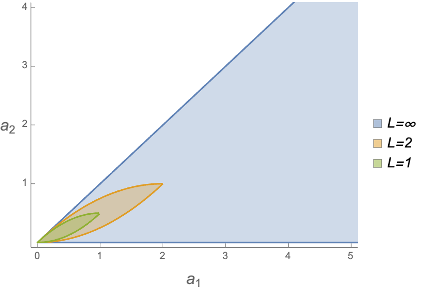
Refer to caption — Figure 1: The allowed space for single $L$ -moments, for $L=1,2,\infty$ . For $L=\infty$ only the projective bounds $0\leq a_{2}/a_{1}\leq 1$ are left.

The next step is to compute the dispersion relation as the Minkowski sum of single $L$ -moments, one for each spin and rescaled by the $\lambda_{\ell,k,q}$ factors. Since the boundary of a Minkowski sum $A+B$ is contained in the Minkowski sum of the boundaries of $A$ and $B$ , we simply take a sum of boundary parametric curves such as eq.(1) and extremize with respect to the parameters. For example, the Minkowski sum of two moments is shown in Figure 2(a).

Remarkably, we find that the Minkowski sum of an infinite number of moments converges in many of our cases of interest, leading to the non-projective EFThedron. This geometric object has an infinite number of distinct facets, each resulting from the Minkowski sum of different subsets of spins. We sketch an example in Figure 2(b).

Using this analytic geometry, we can now derive bounds for individual couplings. For example, for $g_{k,0}$ with $k\in even$ , imposing permutation invariance at eighth derivative order ( $k=4$ ) we reproduce the result for $g_{2,0}$ in Caron-Huot:2020cmc, while for $4\leq k\leq 256$ we find

\frac{g_{k,0}}{(4\pi)^{2}}\leq\frac{2}{k}\left(30-18\left(\frac{35}{36}\right)^{\frac{k}{4}}\right)\frac{1}{\pi^{2}M^{2k}}\,.

(13)

with small corrections for higher $k$ , illustrated in Figure 3. While the leading derivative operators are bounded by $\mathcal{O}(1)$ , subsequent operators are in fact suppressed as $1/k$ for $k\gg 1$ . Such results are stronger than the combination of non-projective bounds for a single operator and projective bounds for the remaining, which would only imply $g_{k,0}\leq g_{k,2}$ . In Figure 4 we compare this bound with the EFT coefficients arising from the UV amplitude of a massive scalar at one loop.

The massive scalar satisfies the bound due to combinatorics from expanding the loop integrand at low energies. Similar to the projective geometry, in higher dimensional spaces we can derive analytic expressions for the boundaries, which we compare to numerical results from linear programming (LP), as well as previously known projective bounds. For example, with permutation invariance imposed at $k=4$ , we obtain Figure 5.

The paper is organized as follows. In Section 2 we find the non-projective polytope resulting from the Minkowski sum of finite segments. In addition to describing the space of couplings at equal mass dimension, we then show how this result can be used to solve the single $L$ -moment problem. We present other aspects of the $L$ moment problem, including Hankel constraints, in Appendix A. In Section 3 we compute the Minkowski sum of single $L$ moments. This is carried out by extremizing the sum using Lagrange multipliers, but we also discuss an alternative solution in Appendix B. We solve this problem completely in 2D. For higher dimensions we present closed form solutions for particular cases. In Appendix C we discuss how this approach could be extended to more general cases. In Section 4 we apply the results to obtain physical bounds on the scattering amplitude of four massless scalars. Although not directly applicable to our four scalar amplitude, in Appendix D we show how the previous results can be used to impose the low spin dominance condition. We conclude in Section 5.

2 De-projection of convex hulls

As reviewed in the previous section, the dispersive representation of EFT coefficients generally takes the form

a_{k,q}=\sum_{\ell\in\mathbb{N}}v_{\ell,k,q}\int_{0}^{1}\rho_{\ell}(z)z^{k-1}dz,\quad 0\leq\rho_{\ell}(z)\leq 2\,.

(14)

When we neglect the upper bound on $\rho_{\ell}$ , the space for allowed $a_{k,q}$ is projective and one can only bound the ratios of $a_{k,q}$ . The corresponding projective space is characterized by the convex hull of product moments as described in Arkani-Hamed:2020blm; Chiang:2021ziz.

To incorporate the effects of the upper bound, we will view the geometry as the Minkowski sum of convex hulls. To illustrate this point, we will first consider a simplified version of eq.(14) where the coefficients $v_{\ell,k,q}$ are independent of $k$ , and the vectors

{\bf v}_{\ell}=\begin{pmatrix}v_{\ell,q_{1}}\\ v_{\ell,q_{2}}\\ \vdots\\ v_{\ell,q_{D}}\end{pmatrix}\,,

(15)

are cyclically ordered by $\ell$ in the sense that,

\textrm{det}\begin{pmatrix}{\bf v}_{i_{1}}&{\bf v}_{i_{2}}&{\bf v}_{i_{3}}&\ldots\end{pmatrix}\equiv\langle i_{1},i_{2},i_{3},\cdots i_{D}\rangle\geq 0,\quad\forall i_{1}<i_{2}<i_{3}\cdots<i_{D}\,.

(16)

We begin with the space of couplings with equal $k$ (“same mass-dimension”),

(a_{k,q_{1}},a_{k,q_{2}},\cdots)\,,

(17)

whose projective geometry is simply that of a cyclic polytope. We will show that the “de-projected” space can be constructed by taking the Minkowski sum of line segments, resulting in a convex polytope whose vertices are given by linear sums of successive ${\bf v}_{\ell}$ s.

This result will allow us to derive the boundaries for a closely related geometry: the $L$ -moment problem. This concerns the space of $a_{k}$ given by

a_{k}=\int_{0}^{1}\rho_{\ell}(z)z^{k-1}dz,\quad 0\leq\rho_{\ell}(z)\leq L\,.

(18)

The limit $L\rightarrow\infty$ corresponds to the Hausdorff moment problem, whose solution is given by the positivity of Hankel matrices constructed from $a_{k}$ . We will derive the solutions for finite $L$ .

2.1 Minkowski sums

In this section we review some basic notions related to Minkowski sums. Let us consider two regions $A,B$ with each point inside the regions defined by a vector. The Minkowski sum of the two regions is then given by all possible pairs of vectors, one from $A$ and one from $B$ , and taking their sum:

A{+}B=\{a{+}b,\forall a\in A,\forall b\in B\}\,.

(19)

It can be understood as translating the region $B$ by all vectors $a\in A$ , or vice versa. As an example consider $A$ and $B$ to be separate disks shown in Figure 6. Their Minkowski sum is then displayed as the light blue region, which contains any vector in $B$ shifted by all vectors in $A$ .

We will be interested in characterizing this sum in terms of its boundaries $\partial(A{+}B)$ , which are determined by the individual boundaries $\partial A$ and $\partial B$ . More precisely, any vector on $\partial(A{+}B)$ must be comprised by the sum of a vector on $\partial A$ and a vector on $\partial B$ . However the reverse is not necessarily true, as illustrated in the above figure, where a sum of boundary vectors sits inside the Minkowski sum. In fact, the boundary of the Minkowski sum $A{+}B$ is a subset of boundaries for the Minkowski sum $\partial A{+}\partial B$ . Indeed for our example in Figure 7, the Minkowski sum of $\partial A$ (denoted by the red contour) and $\partial B$ (denoted by the blue contour) covers a subregion of $A{+}B$ which contains two boundaries, with the outer one being $\partial(A{+}B)$ . Thus when one is interested in the boundary of the Minkowski sum, only the boundaries of the individual sets are relevant.

Let us take a simpler example which will be of immediate use. Consider the Minkowski sum of three segments labeled $1,2,3$ in Figure 8. The boundary of each segment is given by the end points. Thus following the discussion above, the boundary of the Minkowski sum is given by the Minkowski sum of the end points, i.e. three vectors. In this case, the vectors are labeled according to their slope, and thus the boundary can be sequentially constructed by starting with the vector with the smallest slope, and successively adding the next vector until all vectors are included. Then one starts subtracting the first vector and so forth until one is left with the vector of the largest slope.

2.2 De-projecting the cyclic polytope

Let us begin with

a_{k,q}=\sum_{\ell}v_{\ell,q}\int_{0}^{1}\rho(z)z^{k-1}dz=\sum_{\ell}v_{\ell,q}a_{k}^{(\ell)}=\sum_{\ell}a_{k,q}^{(\ell)}\,,

(20)

where $\rho(z)$ is bounded as $0\leq\rho(z)\leq L$ . Note that each $a_{k}^{(\ell)}$ is a 1D segment, $0\leq a_{k}^{(\ell)}\leq\frac{L}{k}$ . For later convenience we will parameterize the segments as

a_{k}^{(\ell)}=m_{\ell}\frac{L}{k},\quad m_{\ell}\in[0,1]\,.

(21)

The combination

{\bf a}^{(\ell)}=\begin{pmatrix}a_{k,q_{1}}^{(\ell)}\\ a_{k,q_{2}}^{(\ell)}\\ \vdots\\ a_{k,q_{D}}^{(\ell)}\end{pmatrix}=m_{\ell}\frac{L}{k}\begin{pmatrix}v_{\ell,q_{1}}\\ v_{\ell,q_{2}}\\ \vdots\\ v_{\ell,q_{D}}\end{pmatrix}=m_{\ell}{\bf v}_{\ell}\,,

(22)

then represents a segment in $D$ dimensions, also parameterized by $m_{\ell}$ . Eq.(20) is therefore

{\bf a}\equiv\sum_{\ell}m_{\ell}{\bf v}_{\ell}

(23)

that is, ${\bf a}$ corresponds to a Minkowski sum of segments, with endpoints $(0,0,\cdots,0)$ and ${\bf v}_{\ell}=\frac{L}{k}(v_{\ell,q_{1}},v_{\ell,q_{2}},\cdots,v_{\ell,q_{D}})$ in $D$ dimensions. As discussed previously, the boundary of the Minkowski sum ${\bf a}$ is found from the Minkowski sum of the boundaries of ${\bf a}^{(\ell)}$ . Therefore the endpoints of the segments, represented by vectors ${\bf v}_{\ell}$ will be what is relevant to the problem.

Two dimensions

Let us start in two dimensions, where the $N$ ordered vectors ${\bf v}_{\ell}$ satisfy

\langle i_{1},i_{2}\rangle>0,\quad\forall i_{1}<i_{2}\,.

(24)

As a consequence the relative angle of any two vectors is less than $\pi$ , and they span at most a half space. From the example in the beginning of this section, it is straightforward to determine that the Minkowski sum is a polygon with $2N$ ordered vertices ${\bf V}_{i}=\sum_{j<i}{\bf v}_{j}$ and $\bar{\bf V}_{i}=\sum_{j>i}{\bf v}_{j}$ , $1\leq i\leq N$ . This region can be characterized by the inequalities

{\rm det}\left(\begin{array}[]{ccc}1&1&1\\ {\bf a}&{\bf V}_{i}&{\bf V}_{i+1}\end{array}\right),\quad{\rm det}\left(\begin{array}[]{ccc}1&1&1\\ {\bf a}&\bar{{\bf V}}_{i}&\bar{{\bf V}}_{i+1}\end{array}\right)\geq 0,\quad\,1\leq i\leq N\,.

(25)

where we have ${\bf V}_{1}=\bar{{\bf V}}_{N{+}1}={\bf 0}$ . Note that the boundaries are non-linear in ${\bf a}$ , since the geometry is non-projective. As an example the Minkowski sum with $N=2,3,4$ vectors are displayed in Figure 9.

In higher dimensions we can derive the boundaries by projecting the Minkowski sum to 1D. Each projection will give necessary constraints corresponding to two of the co-dimension 1 boundaries. Let us use the 2D example as an illustration. We project all the vectors ${\bf v}_{\ell}$ to the one-dimensional line orthogonal to one of the vectors, say ${\bf v}_{i}$ . The end-points of the projected segments are now given by $0$ and

v_{j}^{(i)}\equiv\frac{1}{|{\bf v}_{i}|}\langle j,i\rangle\,.

(26)

If the vectors satisfy eq.(24), the projections are oriented according to the ordering: segments corresponding to $1\leq j\leq i$ are in the negative direction, while segments corresponding to $i\leq j\leq N$ are in the positive direction.³³ 3 Note that for notational simplicity, we are considering ${\bf v}_{i}$ to be part of both sets. Including it or not does not change any of the equations, since ${\bf v}_{i}^{(i)}=0$ . This projection is shown in Figure 10.

The end points of the 1D Minkowski sum are then simply the sum over the 1D vectors on either side respectively:

	$\displaystyle{V}^{(i)}_{1,i}$	$\displaystyle\equiv$	$\displaystyle\sum_{j\leq i}{v}_{j}^{(i)}=\sum_{j\leq i}\frac{1}{\|{\bf v}_{i}\|}\langle j,i\rangle=\frac{1}{\|{\bf v}_{i}\|}\langle{\bf V}_{1,i},i\rangle\,,$
	$\displaystyle{V}_{i,N}^{(i)}$	$\displaystyle\equiv$	$\displaystyle\sum_{j\geq i}{v}_{j}^{(i)}=\frac{1}{\|{\bf v}_{i}\|}\langle{\bf V}_{i,N},i\rangle\,,$		(27)

where we have defined ${\bf V}_{i_{1},i_{2}}=\sum_{j=i_{1}}^{i_{2}}{\bf v}_{j}\,$ . The last form indicates that a 1D end point is the projection of one of the vertices of the whole 2D Minkowski sum, as it must. Now a necessary condition for any point ${\bf a}$ to be inside the Minkowski sum is that its projection through ${\bf v}_{i}$ must lie within the $1D$ boundaries. This implies

\langle{\bf V}_{i,N},i\rangle\leq\langle{\bf a},i\rangle\leq\langle{\bf V}_{1,i},i\rangle\,.

(28)

We obtain two boundaries, which we denote as

	$\displaystyle P_{i}^{\textrm{lower}}$	$\displaystyle\equiv$	$\displaystyle-\langle{\bf a}{-}{\bf V}_{1,i},i\rangle=\textrm{det}\begin{pmatrix}1&1&1\\ {\bf a}&{\bf V}_{1,i}&{\bf V}_{1,i}\end{pmatrix}_{3\times 3}\geq 0\,,$
	$\displaystyle{P}_{i}^{\textrm{upper}}$	$\displaystyle\equiv$	$\displaystyle\langle{\bf a}{-}{{\bf V}}_{i,N},i\rangle=\textrm{det}\begin{pmatrix}1&1&1\\ {\bf a}&{{\bf V}}_{i,N}&{{\bf V}}_{i,N}\end{pmatrix}_{3\times 3}\geq 0\,,$		(29)

matching the boundaries in eq.(25). Successively repeating the same operation for each vector ${\bf v}_{i}$ then yields the complete set of boundaries. Throughout this paper, we will often refer to boundaries as either upper or lower, labeled in terms of how they would appear in plots. There is however a more invariant definition: given a set of ordered segments, the vertices of the lower boundary are obtained from the successive sum starting from the beginning of the ordering, while the upper boundaries are from the successive sum starting from the end of the ordering. This is apparent from eq.(28). In higher dimensions the equivalent distinction will be such that the upper boundary is the one containing ${\bf V}_{i,N}$ (regardless of whether it also contains ${\bf V}_{1,i}$ ).

To check these boundaries are correct and can also be saturated, we can substitute ${\bf a}$ by its general form in eq.(23), ${\bf a}=\sum_{j}m_{j}{\bf v}_{j}$ , where $0\leq m_{j}\leq 1$ . Since ${\bf a}{-}{\bf V}_{1,i}=\sum_{j<i}(m_{j}{-}1){\bf v}_{j}{+}\sum_{i\geq j}m_{j}{\bf v}_{j}$ , the determinant in eq.(2.2) then becomes

P_{i}=\sum_{j<i}(1-m_{j})\langle j,i\rangle-\sum_{j>i}m_{j}\langle j,i\rangle\,.

(30)

Due to the cyclic condition, we have that $\langle j,i\rangle$ is positive for $j<i$ , and negative for $j>i$ , therefore the expression above is non-negative term by term. These are true boundaries since the equality $P_{i}=0$ can be saturated by taking $m_{j}=1$ for $j<i$ and $m_{j}=0$ for $j>i$ , while $m_{i}$ can be any value between 0 and 1, parameterizing the edge between vertices $i$ and $i+1$ .

3D

We next consider three-dimensional vectors, which we again assume satisfy the ordering of eq.(16). We will derive the boundary by considering two successive projections down to 1D, through two vectors ${\bf v}_{i_{1}}$ and ${\bf v}_{i_{2}}$ , for $i_{1}<i_{2}$ . Since the vectors are ordered, we deduce:

\displaystyle\begin{array}[]{c}\langle j,i_{1},i_{2}\rangle>0\,,\quad j{<}i_{1}{<}i_{2}\,,\\ \langle j,i_{1},i_{2}\rangle<0\,,\quad i_{1}{<}j{<}i_{2}\,,\\ \langle j,i_{1},i_{2}\rangle>0\,,\quad i_{1}{<}i_{2}{<}j\,.\end{array}

That is, when projecting twice down to 1D, the remaining $N{-}2$ vectors will be split into two sets: the vectors ${\bf v}_{i_{1}{+}1},{\bf v}_{i_{1}{+}2},\ldots,{\bf v}_{i_{2}{-}1}$ yield points on one side, and ${\bf v}_{i_{2}{+}1},{\bf v}_{i_{2}{+}2},\ldots,{\bf v}_{i_{1}{-}1}$ on the other.⁴⁴ 4 The ordering is cyclic, thus ${\bf v}_{N{+}1}\equiv{\bf v}_{1}$ . The resulting end points of the one-dimensional Minkowski sum are then given by summing over the vectors in the respective sets. By requiring any point in the Minkowski sum to lie between the two endpoints we obtain

\langle{\bf V}_{i_{1},i_{2}},i_{1},i_{2}\rangle\leq\langle{\bf a},i_{1},i_{2}\rangle\leq\langle{\bf V}_{1,i_{1}}{+}{\bf V}_{i_{2},N},i_{1},i_{2}\rangle\,,

(35)

	$\displaystyle P_{i_{1},i_{2}}$	$\displaystyle\equiv$	$\displaystyle\langle{\bf a}{-}{\bf V}_{i_{1},i_{2}},i_{1},i_{2}\rangle\geq 0,\,$
	$\displaystyle\overline{P}_{i_{1},i_{2}}$	$\displaystyle\equiv$	$\displaystyle{-}\langle{\bf a}{-}{\bf V}_{1,i_{1}}{-}{\bf V}_{i_{2},N},i_{1},i_{2}\rangle\geq 0\,.$		(36)

The complete boundary is then given by the collection of $P_{i_{1},i_{2}},\overline{P}_{i_{1},i_{2}}$ for all pairs of $\{i_{1}<i_{2}\}$ . We present an example with $N=5$ vectors in Figure 11. Note that in this case we refer to $\overline{P}$ as the upper boundary, as it contains ${\bf V}_{i_{2},N}$ .

General dimension

In $D$ dimensions each boundary is labeled by $D{-}1$ indices, corresponding to the $D-1$ vectors we use to project. We denote this set as $I=(i_{1},i_{2},i_{3},\ldots i_{D-1})$ , $1{\leq}i_{1}{<}i_{2}{<}\ldots{<}i_{D-1}{\leq}N$ . Now we must compute, for a given set of projections $I$ , whether a vector ${\bf v}_{j}$ has positive or negative projection. Let

\displaystyle\mathcal{I}^{-}=\{j|v_{j}^{(I)}\leq 0\},\quad\mathcal{I}^{+}=\{j|v_{j}^{(I)}\geq 0\},

(37)

If the ${\bf v}$ are ordered, we have, for $D=\textrm{even}$ :

	$\displaystyle\mathcal{I}^{-}$	$\displaystyle=$	$\displaystyle[1,i_{1}]\cup[i_{2},i_{3}]\cup\ldots\cup[i_{D-2},i_{D-1}]$
	$\displaystyle\mathcal{I}^{+}$	$\displaystyle=$	$\displaystyle[i_{1},i_{2}]\cup[i_{3},i_{4}]\cup\ldots\cup[i_{D-1},i_{D}]$		(38)

and for $D=\textrm{odd}$ :

	$\displaystyle\mathcal{I}^{-}$	$\displaystyle=$	$\displaystyle[i_{1},i_{2}]\cup[i_{3},i_{4}]\cup\ldots\cup[i_{D-2},i_{D-1}]$
	$\displaystyle\mathcal{I}^{+}$	$\displaystyle=$	$\displaystyle[1,i_{1}]\cup[i_{2},i_{3}]\cup\ldots\cup[i_{D-1},i_{N}]$		(39)

To maintain our convention that the upper boundary, corresponding to the $\overline{P}_{I}\geq 0$ , is the one containing ${\bf v}_{N}$ , we then define ${\bf V}_{I}$ and ${\bf\overline{V}}_{I}$ such that for $D=\textrm{even}$ :

	$\displaystyle\textrm{lower:}\quad{\bf V}_{I}$	$\displaystyle\equiv\displaystyle\sum_{i\in\mathcal{I}^{+}}{\bf v}_{j}=$	$\displaystyle{\bf V}_{1,i_{1}}+{\bf V}_{i_{2},i_{3}}+\ldots{\bf V}_{i_{D-2},i_{D-1}}\,,$
	$\displaystyle\textrm{upper:}\quad{\bf\overline{V}}_{I}$	$\displaystyle\equiv\displaystyle\sum_{i\in\mathcal{I}^{-}}{\bf v}_{j}=$	$\displaystyle{\bf V}_{i_{1},i_{2}}+{\bf V}_{i_{3},i_{4}}+\ldots{\bf V}_{i_{D-1},N}\,,$		(40)

and for $D=\textrm{odd}$ :

	$\displaystyle\textrm{lower:}\quad{\bf V}_{I}$	$\displaystyle\equiv\displaystyle\sum_{i\in\mathcal{I}^{-}}{\bf v}_{j}=$	$\displaystyle{\bf V}_{i_{1},i_{2}}+{\bf V}_{i_{3},i_{4}}+\ldots{\bf V}_{i_{D-2},i_{D-1}}\,,$
	$\displaystyle\textrm{upper:}\quad{\bf\overline{V}}_{I}$	$\displaystyle\equiv\displaystyle\sum_{i\in\mathcal{I}^{+}}{\bf v}_{j}=$	$\displaystyle{\bf V}_{1,i_{1}}+{\bf V}_{i_{2},i_{3}}+\ldots{\bf V}_{i_{D-1},N}\,.$		(41)

Then we have the constraints

	$\displaystyle P_{I}$	$\displaystyle=$	$\displaystyle(-1)^{D+1}\langle{\bf a}{-}{\bf V}_{I},i_{1},i_{2},\ldots,i_{D{-}1}\rangle\,,$
	$\displaystyle\overline{P}_{I}$	$\displaystyle=$	$\displaystyle(-1)^{D}\langle{\bf a}{-}{\bf\overline{V}}_{I},i_{1},i_{2},\ldots,{i_{D{-}1}}\rangle\,.$		(42)

By considering all possible choices $1\leq i_{1}{<}i_{2}{<}\ldots{<}i_{D-1}{\leq}N$ we obtain the complete boundary.

Non-cyclic vectors

In the case where the ${\bf v}$ s cannot be cyclically ordered, then we no longer know beforehand whether the 1D projection of any vector will be positive or negative. Therefore, eqns.(2.2) and (2.2) no longer necessarily follow from the definition in eq.(37). In such case one has to individually check, for every sequence $I$ , which vectors ${\bf v}$ belong to which set, $\mathcal{I}^{+}$ or $\mathcal{I}^{-}$ , and use this to compute ${\bf V}$ and ${\bf\overline{V}}$ . In practice, since we are usually interested in intersecting the geometry with a null constraint, typically this means only a finite number of boundaries are relevant, so this is a trivial computational task.

In two dimensions only vectors spanning more than a half-plane cannot be cyclically ordered, and the problem can be solved straightforwardly. We first pick a half-plane,⁵⁵ 5 In the physical problem, there will be an infinite number of vectors, but always accumulating in a single quadrant. In this case we must pick the half-plane including this quadrant. and name the vectors in this half-plane ${\bf v}$ , and the remaining ${\bf\tilde{v}}$ . The Minkowski sum is now

{\bf a}=\sum_{i}m_{i}{\bf v_{i}}+\sum_{i}m_{i}{\bf\tilde{v}_{i}}\,.

(43)

Next we add and subtract $\sum_{i}{\bf\tilde{v}}_{i}$ . Since the sum is associative, we can group this as

{\bf a}=\left(\sum_{i}m_{i}{\bf v_{i}}+\sum_{i}(m_{i}-1){\bf\tilde{v}_{i}}\right)+\sum_{i}{\bf\tilde{v}_{i}}\,.

(44)

The combinations $(m_{i}-1){\bf\tilde{v}_{i}}$ are now segments in the same half-plane as the ${\bf v}$ , so the sum in parantheses can be computed as before, simply ordering the vectors according to their slope $v_{\ell,k_{2},q_{2}}/v_{\ell,k_{1},q_{1}}$ , regardless of what half-plane they are in. Finally we translate the whole boundary by $\sum_{i}{\bf\tilde{v}_{i}}$ .

2.3 De-projecting the moment problem: The $L$ -moment

Let us now consider a different problem, where our previous result will guide us to the answer. We want to find the allowed space of moments $(a_{k_{1}},a_{k_{2}},\ldots)$ that satisfy

a_{k}=\int_{0}^{1}\rho(z)z^{k-1}dz,\quad 0\leq\rho(z)\leq L\,.

(45)

This is known as the “ $L$ -moment problem” akhiezer1934fouriersche; akhiezer1962some. We will solve it in a straightforward fashion by taking the continuous limit of the polytope discussed in the previous section. To relate the two we express the above integral as a Riemann sum

a_{k}=\int_{0}^{1}\rho(z)z^{k-1}dz\;\rightarrow\;\sum_{i=1}^{N}\rho_{i}\frac{i^{k-1}}{N^{k}}\,,

(46)

where $\rho_{i}\equiv\rho(i/N)\leq L$ , which again we can consider to be a segments of length $L$ , parameterized by $m_{i}\in[0,1]$ . We can then write the above as

a_{k}=\sum_{i=1}^{N}m_{i}v_{i,k}

(47)

where $v_{i,k}=Li^{k-1}/N^{k}$ . Expressed as a discrete sum the $L$ moment problem is equivalent to a Minkowski sum of segments, with endpoints at 0 and $L(v_{i,k_{1}},v_{i,k_{2}},\ldots)$ . Furthermore, the $v_{i,k}$ are ordered, as taking a collection of $N$ such vectors the resulting $N\times N$ determinant will be proportional to the Vandermonde determinant, and thus eq.(16) holds. The results in the previous section therefore apply to this case, so the vertices of the Minkowski sum in eq.(47) are given by eq.(2.2). As we take $N\rightarrow\infty$ , the infinite number of polytope boundaries merge into a smooth curve and each vertex is a point on the curve.

Two dimensions Let us take the two dimensional space $(a_{k_{1}},a_{k_{2}})$ as an example. From the previous subsection, the vertices are

{V}_{1,i|k}=L\sum_{j=1}^{i}v_{j,k}=L\sum_{j=1}^{i}\frac{j^{k-1}}{N^{k}}\,.

(48)

Now we define $m\equiv\frac{i}{N}\in[0,1]$ and $z\equiv\frac{j}{N}\in[0,m]$ , which in the $N\rightarrow\infty$ limit can be treated as continuous parameters. The sum in eq.(48) simply becomes an integral

{V}_{1,i|k}=L\sum_{j=1}^{i}\frac{j^{k-1}}{N^{k}}\rightarrow L\int_{0}^{m}z^{k-1}dz=L\frac{m^{k}}{k}\,,

(49)

and the boundary vertex becomes a point on the parametric curve

(a_{k_{1}},a_{k_{2}})=({U}_{k_{1}}(m),{U}_{k_{2}}(m)),\quad{U}_{k}(m)\equiv L\frac{m^{k}}{k}\,.

(50)

Similarly for the vertices of type ${\bf V}_{i,N}$ in the continuous limit we obtain:

(a_{k_{1}},a_{k_{2}})=(\overline{U}_{k_{1}}(m),\overline{U}_{k_{2}}(m)),\quad\overline{U}_{k}(m)\equiv L\frac{1-m^{k}}{k}\,.

(51)

Note that we can rephrase the boundary as a particular solution for $\rho(z)$ . It is not hard to work out that the solution for lower and upper boundary are given by

	$\displaystyle{\rm lower}:\quad\rho(z)$	$\displaystyle=$	$\displaystyle\chi_{I}(z),\;\;I=[0,m]$
	$\displaystyle{\rm upper}:\quad\rho(z)$	$\displaystyle=$	$\displaystyle\chi_{I}(z),\;\;I=[m,1]$

where $\chi_{I}(z)=L$ for $z\in I$ and zero otherwise. In other words, the boundary solutions are constants along some region in $z$ ! To find the constraint equations in $a_{k}$ that describe the boundary, we simply combine the couplings in such a way that removes the boundary parameter. Then the allowed space can be expressed as an inequality

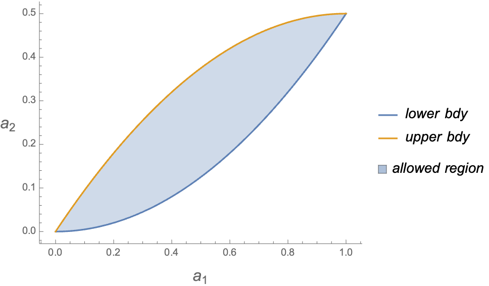
\displaystyle\frac{L}{k_{2}}\left(\frac{k_{1}}{L}a_{k_{1}}\right)^{\frac{k_{2}}{k_{1}}}\leq a_{k_{2}}\leq\frac{L}{k_{2}}\bigg(1-\left(1-\frac{k_{1}}{L}a_{k_{1}}\right)^{\frac{k_{2}}{k_{1}}}\bigg)\,.

(52)

This represents the allowed space for the 2D $L$ moment problem. We plot this in Figure 12, for $k_{1}=1,k_{2}=2$ and for $L=1,2,\infty$ , observing the $L=\infty$ limit reproduces the projective bounds of the usual moment problem, namely $0\leq\frac{a_{k_{2}}}{a_{k_{1}}}\leq 1$ .

Three dimensions In 3D the same procedure gives the boundary as a parametric surface. Taking the continuous limit of a vertex ${\bf V}_{i_{1},i_{2}}$ we find the boundary is

	$\displaystyle(a_{k_{1}},a_{k_{2}},a_{k_{3}})$	$\displaystyle=$	$\displaystyle(U_{k_{1}}(m_{1},m_{2}),U_{k_{2}}(m_{1},m_{2}),U_{k_{3}}(m_{1},m_{2})),$
	$\displaystyle U_{k}(m_{1},m_{2})$	$\displaystyle\equiv$	$\displaystyle\frac{L}{k}\left(m_{2}^{k}{-}m_{1}^{k}\right)\,,$		(53)

while for the upper boundary one has $\overline{U}_{k}(m_{1},m_{2})\equiv\frac{L}{k}\left(1{-}m_{2}^{k}{+}m_{1}^{k}\right)$ . The boundary distribution is given by

	$\displaystyle{\rm Lower}:\quad\rho(z)$	$\displaystyle=$	$\displaystyle\chi_{I}(z),\;\;I=[m_{1},m_{2}],$
	$\displaystyle{\rm Upper}:\quad\rho(z)$	$\displaystyle=$	$\displaystyle\chi_{I_{1}}(z){+}\chi_{I_{2}}(z),\;\;I_{1}=[0,m_{1}],\;\;I_{2}=[m_{2},1],\,.$

For a space $(a_{1},a_{2},a_{3})$ the two boundaries lead to the inequalities:

\displaystyle\frac{a_{1}^{4}+12L^{2}a_{2}^{2}}{12L^{2}a_{1}}\leq a_{3}\leq\frac{a_{1}^{4}-4La_{1}^{3}+6L^{2}a_{1}^{2}+12L^{2}a_{2}^{2}-12L^{3}a_{2}}{12L^{2}(a_{1}-L)}\,.

(54)

The explicit region is shown in Figure 13. The generalization to higher dimensions can be readily obtained from eqs.(2.2) and (2.2), by replacing all terms ${\bf V}_{i_{1},i_{2}}\rightarrow{\bf U}(m_{1},m_{2})$ . Explicitly, we obtain

	$\displaystyle\textrm{lower: }U_{k}$	$\displaystyle=$	$\displaystyle\frac{L}{k}\sum_{i=1}^{D-1}(-1)^{i+1}m_{i}^{k}\,$
	$\displaystyle\textrm{upper: }\overline{U}_{k}$	$\displaystyle=$	$\displaystyle\frac{L}{k}\left(1-\sum_{i=1}^{D-1}(-1)^{i+1}m_{i}^{k}\right)\,.$		(55)

Note that the inequalities above are non-projective, i.e. they involve polynomials of $a_{k}$ with different degrees. This is different from the usual moment problem where the constraints are given by the positivity of Hankel matrices, which are homogenous in the degree of couplings. However, through a set of non-linear (exponential) maps to new couplings, the constraints can again be expressed through the positivity of Hankel matrices. In fact this is how the solution to the $L$ -moment problem is usually given in the literature, which we review in Appendix A. For our purpose, the parametric form of the boundary will be more useful, as we will perform further Minkowski sums for the general problem.

3 Minkowski sums of single $L$ -moments

We now return to the our general problem

a_{k,q}=\sum_{\ell}v_{\ell,k,q}\int_{0}^{1}\rho_{\ell}(z)z^{k-1},\quad 0\leq\rho_{\ell}\leq L\,.

(56)

We will solve this problem by treating the $a_{k,q}$ as yet another Minkowski sum. We can write the above as

\begin{pmatrix}a_{k_{1},q_{1}}\\ a_{k_{1},q_{2}}\\ \vdots\\ a_{k_{D},q_{D}}\end{pmatrix}=\sum_{\ell}\begin{pmatrix}a_{k_{1},q_{1}}^{(\ell)}\\ a_{k_{2},q_{2}}^{(\ell)}\\ \vdots\\ a_{k_{D},q_{D}}^{(\ell)}\end{pmatrix}=\sum_{\ell}\begin{pmatrix}a_{k_{1}}^{(\ell)}v_{\ell,k_{1},q_{1}}\\ a_{k_{2}}^{(\ell)}v_{\ell,k_{2},q_{2}}\\ \vdots\\ a_{k_{D}}^{(\ell)}v_{\ell,k_{D},q_{D}}\end{pmatrix}\,.

(57)

where for each spin, the $a_{k,q}^{(\ell)}$ is identified as the solution to the $L$ -moment problem $a_{k}=(a_{k_{1}},a_{k_{2}},\ldots,a_{k_{D}})$ , with each component $a_{k_{i}}$ rescaled by some number $v_{\ell,k_{i},q_{i}}$ . The full geometry is then given by the Minkowski sum over all spins of such geometries.

As discussed in the beginning of the previous section, to compute the boundary of the Minkowski sum, one first computes the Minkowski sum of the boundaries. The final boundary can be found by extremizing this result, most simply using Lagrange multipliers, as we will discuss shortly. Alternatively we can revert the $L$ -moment problem to its discrete version, and simply consider the whole problem as a double Minkowski sum of segments. We will explore this view point in detail in appendix B. Here we will present the result from the Lagrange method.

We first solve the problem for any 2D space $(a_{k_{1},q_{1}},a_{k_{2},q_{2}})$ , for any $v_{\ell,k,q}$ . This will be sufficient to derive optimal bounds on any 2D space of couplings without imposing null constraints, or bounds on any single coupling with one null constraint.

To implement more null constraints, or to obtain obtain the space of more couplings, would require us to solve the geometry in higher dimensions. In this case we only obtain partial results. First, we can easily derive boundaries when only a a finite number of spins are relevant. When the sum over infinite spins cannot be avoided, we are only able to find closed form expressions for spaces $(a_{k_{1},q_{1}},a_{k_{2},q_{2}},\ldots)$ satisfying $k_{i+1}{-}k_{i}{=}\Delta_{k}$ , $q_{i+1}{-}q_{i}{=}\Delta_{q}$ , and when $v_{\ell,k,q}{=}v_{\ell,q}{=}g(\ell)f(\ell)^{q}$ , where $g(\ell)$ and $f(\ell)$ can be general polynomials of $\ell$ .

For the entire space of couplings, the problem can be formulated in terms of envelopes of various moment constraints. This is more amendable to numerical approaches which we explore in appendix C.

3.1 Extremizing the Minkowski sum

In this section we briefly explain how the boundary of a Minkowski sum can be obtained by extremizing. Let us use the example of the disks in Figure 7 to introduce this method. We can describe the boundaries of disks A and B as

	$\displaystyle\partial A(\theta_{A})$	$\displaystyle=$	$\displaystyle(a_{x},a_{y})+r_{A}(\textrm{sin}\theta_{A},\textrm{cos}\theta_{A})\,,$
	$\displaystyle\partial B(\theta_{B})$	$\displaystyle=$	$\displaystyle(b_{x},b_{y})+r_{B}(\textrm{sin}\theta_{B},\textrm{cos}\theta_{B})\,,$		(58)

The Minkowski sum of boundaries $\partial A(\theta_{A})+\partial B(\theta_{B})$ is then a 2D region, with the two components given by

	$\displaystyle f_{x}(\theta_{A},\theta_{B})$	$\displaystyle=$	$\displaystyle(a_{x}{+}b_{x}){+}r_{A}\textrm{sin}\,\theta_{A}{+}r_{B}\textrm{sin}\,\theta_{B}$
	$\displaystyle f_{y}(\theta_{A},\theta_{B})$	$\displaystyle=$	$\displaystyle(a_{y}{+}b_{y}){+}r_{A}\textrm{cos}\,\theta_{A}{+}r_{B}\textrm{cos}\,\theta_{B}\,.$		(59)

To find the boundary of this region we can consider extremizing in one coordinate while the other is held fixed. This gives a constraint equation that will allow us to solve one parameter in terms of the remaining, giving the co-dimension one boundaries of the Minkowski sum $\partial A(\theta_{A})+\partial B(\theta_{B})$ . More precisely, fixing the $x$ -coordinate while extremizing in $y$ , one solves

\left(\begin{array}[]{c}\partial_{\theta_{A}}f_{x}(\theta_{A},\theta_{B})\\ \partial_{\theta_{B}}f_{x}(\theta_{A},\theta_{B})\end{array}\right)=\lambda\left(\begin{array}[]{c}\partial_{\theta_{A}}f_{y}(\theta_{A},\theta_{B})\\ \partial_{\theta_{B}}f_{y}(\theta_{A},\theta_{B})\end{array}\right)\,,

(60)

where $\lambda$ is the Lagrangian multiplier. Note that this is simply saying that the two component vectors are proportional and hence

{\rm det}\left(\begin{array}[]{cc}\partial_{\theta_{A}}f_{x}(\theta_{A},\theta_{B})&\partial_{\theta_{A}}f_{y}(\theta_{A},\theta_{B})\\ \partial_{\theta_{B}}f_{x}(\theta_{A},\theta_{B})&\partial_{\theta_{B}}f_{y}(\theta_{A},\theta_{B})\end{array}\right)=0\;\;\rightarrow\;\;\cos\theta_{A}\sin\theta_{B}=\cos\theta_{B}\sin\theta_{A}\,.

(61)

We find two solutions: $\theta_{A}=\theta_{B}$ and $\theta_{A}=\theta_{B}+\pi$ . These precisely correspond to the outer and inner boundaries in Figure 7, given by

\partial(\partial A+\partial B)=(a_{x}+b_{x},a_{y}+b_{y})+(r_{A}\pm r_{B})(\textrm{sin}\phi_{A},\textrm{cos}\phi_{A})\,.

(62)

This generalizes to higher dimensions. Consider the combination of two $D$ -dimensional regions. We find the boundary of their Minkowski sum by taking the Minkowski sum of the boundary $(f_{x_{1}},f_{x_{2}},\cdots,f_{x_{D}})$ , where $f_{x_{i}}$ is a function of $2(D{-}1)$ boundary variables, $(\theta_{1},\theta_{2},\cdots,\theta_{2D{-}2})$ . Holding $(f_{x_{2}},\cdots,f_{x_{D}})$ fixed and extremizing $f_{x_{1}}$ we solve

\left(\begin{array}[]{c}\partial_{\theta_{1}}f_{x_{1}}\\ \partial_{\theta_{2}}f_{x_{1}}\\ \vdots\\ \partial_{\theta_{2(D{-}1)}}f_{x_{1}}\end{array}\right)=\sum_{i=2}^{D}\lambda_{i}\left(\begin{array}[]{c}\partial_{\theta_{1}}f_{x_{i}}\\ \partial_{\theta_{2}}f_{x_{i}}\\ \vdots\\ \partial_{\theta_{2(D{-}1)}}f_{x_{i}}\end{array}\right)\,.

(63)

This gives us $2D{-}2$ constraints on $D{-}1$ Lagrangian multipliers $\lambda_{i}$ and $2(D{-}1)$ boundary variables $\theta_{i}$ , giving us $D{-}1$ -dimensional boundaries.

Finally we comment that since the Lagrange method relies on the variation of the individual boundaries, it will miss boundaries coming from the end points (or boundary of boundaries). These end point contributions must be analyzed by hand, which we will demonstrate through explicit examples.

3.2 Two dimensions with $k_{1}{\neq}k_{2}$

Let us consider first the sum of two moments

a_{k,q}=v_{\ell_{1},k,q}a_{k}^{(\ell_{1})}+v_{\ell_{2},k,q}a_{k}^{(\ell_{1})}=a_{k,q}^{(\ell_{1})}+a_{k,q}^{(\ell_{2})}\,,

(64)

where $a_{k}^{(\ell)}$ takes the form of eq.(45). First, we note that $a_{k,q}^{(\ell)}$ simply represents a single $L$ -moment $a_{k}$ , with each component rescaled by some number $v_{\ell,k,q}$ . This implies the boundaries of $a_{k,q}^{(\ell)}$ are also the original boundaries of $a_{k}$ that we found in Section 2.3, with each component rescaled. We will be considering arbitrary two couplings, $(a_{k_{1},q_{1}},a_{k_{2},q_{2}})$ . The boundary for the $L$ -moment problem in a 2D space $(a_{k_{1}},a_{k_{2}})$ is given by the two curves in eqs.(50) and (51). After the rescaling, we now have:

	lower bdy:		$\displaystyle\quad(a_{k_{1},q_{1}}^{(\ell)},a_{k_{2},q_{2}}^{(\ell)})=L\bigg(\frac{v_{\ell,k_{1},q_{1}}}{k_{1}}m^{k_{1}},\frac{v_{\ell,k_{2},q_{2}}}{k_{2}}m^{k_{2}}\bigg)\,,$
	upper bdy:		$\displaystyle\quad(a_{k_{1},q_{1}}^{(\ell)},a_{k_{2},q_{2}}^{(\ell)})=L\bigg(\frac{v_{\ell,k_{1},q_{1}}}{k_{1}}\left(1{-}m^{k_{1}}\right),\frac{v_{\ell,k_{2},q_{2}}}{k_{2}}\left(1-m^{k_{2}}\right)\bigg)\,.$		(65)

Now eq.(64) requires us to compute the Minkowski sum of such boundaries for different $\ell$ , which we sketch in Figure 14. Note that in principle, we simply need to order the points on the boundaries of $a_{k,q}^{(\ell)}$ , and we can obtain the 2D boundary using the result of the previous section. However for the problem in hand, the proper ordering of points on multiple moments is a cumbersome task. Instead, we will take the boundaries of each $a_{k,q}^{(\ell)}$ and extremize using the Lagrange multiplier as discussed previously. If we assume that all $v_{\ell,k,q}$ s have the same sign, then each moment is oriented in the same “quadrant” and the lower boundary of the Minkowski sum $a_{k,q}$ is contained in the sum of lower boundaries of $a_{k,q}^{(\ell)}$ , and similarly for the upper boundary. If some of the $v_{\ell,k,q}$ have different sign, then special care is needed. We will return to this issue at the end of this section.

Using eq.(3.2) we therefore have that the lower boundary we are after is contained in the 2D region

a_{k,q}(m_{1},m_{2})=\frac{L}{k}\left(v_{\ell_{1},k_{,}q}m_{1}^{k_{1}}+v_{\ell_{2},k_{,}q}m_{2}^{k_{1}}\right),\quad m_{1},m_{2}\in[0,1]\,.

(66)

We can now employ the Lagrange method to find the relation between $m_{1}$ and $m_{2}$ that corresponds to a boundary. The Lagrange equation reads

\nabla_{m_{1},m_{2}}a_{k_{1},q_{1}}=\alpha\nabla_{m_{1},m_{2}}a_{k_{2},q_{2}}\,,

(67)

which implies a remarkably simple relation between the parameters

\frac{m_{1}}{m_{2}}=\left(\frac{v_{\ell_{1},k_{1},q_{1}}}{v_{\ell_{1},k_{2},q_{2}}}\frac{v_{\ell_{2},k_{2},q_{2}}}{v_{\ell_{2},k_{1},q_{1}}}\right)^{\frac{1}{k_{2}-k_{1}}}\equiv r_{1,2}\,.

(68)

Note that $r_{i,j}=r_{j,i}^{-1}$ . If the vectors

{\bf v}_{\ell}=\left(\begin{array}[]{c}v_{\ell,k_{1},q_{1}}\\ v_{\ell,k_{2},q_{2}}\end{array}\right)\,,

(69)

are ordered with respect to spin- $\ell$ , then $r_{i,i-1}\leq 1$ . We can use this to write $m_{2}=r_{2,1}m_{1}$ , which plugging into eq.(66) leads to a boundary curve

a_{k,q}=\frac{L}{k}m_{1}^{k}\left(v_{\ell_{1},k,q}+r_{2,1}^{k}v_{\ell_{2},k,q}\right)\,,

(70)

valid for $m_{1}\in[0,1]$ .

Note that if $m_{1},m_{2}$ are unbounded, then these are the only boundaries. Since they are bounded by $0$ and $1$ , there could exist other boundaries that correspond to fixing one of the parameters to either 0 or 1. There are four possible choices

(m_{1},m_{2})=\{(m,0),(m,1),(0,m),(1,m)\}\,.

(71)

Plugging these into eq.(66) we obtain four curves. We plot these together with the curve in eq.(70) in Figure 15.

We observe that the lower boundary is in fact formed of two sections, corresponding to $a_{k,q}(m,r_{2,1}m)$ and $a_{k,q}(1,m)$

	lower bdy 1:		$\displaystyle a_{k,q}(m,r_{2,1}m)=\frac{L}{k}m^{k}\left(v_{\ell_{1},k,q}+r_{2,1}^{k}v_{\ell_{2},k,q}\right),\quad m\in[0,1]$
	lower bdy 2:		$\displaystyle a_{k,q}(1,m)=\frac{L}{k}\left(v_{\ell_{1},k,q}+m^{k}v_{\ell_{2},k,q}\right),\quad m\in[r_{2,1},1]\,.$		(72)

The lower bound for $m$ in the second section can be understood as follows. The extremized solution is given by the sum of two boundaries in eq.(66) with the relation $m_{2}=r_{2,1}m_{1}$ . The second section starts when $m_{1}$ reaches $1$ , and at that point we have $m_{2}=r_{2,1}m_{1}=r_{2,1}$ .

Next we can perform the same analysis for the upper boundary. In this case the region spanned by the sum of the two upper boundaries is

\overline{a}_{k,q}(m_{1},m_{2})=\frac{L}{k}\left(v_{\ell_{1},k_{,}q_{1}}(1-m_{1}^{k_{1}})+v_{\ell_{2},k_{,}q_{1}}(1-m_{2}^{k_{1}})\right)\,,

(73)

and we find

	upper bdy 1:		$\displaystyle\overline{a}_{k,q}(m,r_{2,1}m),\quad m\in[0,1]$
	upper bdy 2:		$\displaystyle\overline{a}_{k,q}(1,m),\quad m\in[r_{2,1},1]\,.$		(74)

In conclusion, we find the region given by the sum of two moments in Figure 16. Note that as before, the upper boundary is simply a flipped lower boundary, with endpoints matching the (opposite) endpoints of the lower boundary.

For $N$ moments, the above result generalizes by induction. We have the lower boundary contained in the Minkowski sum

a_{k,q}=\frac{L}{k}\sum_{i=1}^{N}v_{\ell_{i},k,q}m_{i}^{k}\,.

(75)

Repeating the arguments from above, we find the lower boundary of a 2D space $(a_{k_{1},q_{1}},a_{k_{2},q_{2}})$ is composed of $N$ sections, where for a section $(j)$ , with $1\leq j\leq N$

	$\displaystyle i<j$	$\displaystyle:$	$\displaystyle\quad m_{i}=1\,,$
	$\displaystyle i\geq j$	$\displaystyle:$	$\displaystyle\quad m_{i}=r_{i,j}m,\quad m\in[r_{j,j-1},1]\,.$		(76)

A section $(j)$ corresponds to the curve

a_{k,q}^{(j)}=\frac{L}{k}\left(G_{k,q}^{(j-1)}+m^{k}v_{\ell_{j},k,q}F_{k,q}^{(j)}\right),\quad m\in[r_{j,j-1},1]\,,

(77)

where $G$ and $F$ are purely numerical factors that depend only on the spin content and the $(k_{1},k_{2},q_{1},q_{2})$ of the space being considered

\displaystyle G_{k,q}^{(j)}=\sum_{i=1}^{j}v_{\ell_{i},k,q}\,,\quad F_{k,q}^{(j)}=\sum_{i=j}^{N}\frac{v_{\ell_{i},k,q}}{v_{\ell_{j},k,q}}r_{i,j}^{k}\,.

(78)

Note that $r_{i,j}$ depends on $(k_{1},q_{1},k_{2},q_{2})$ , so in fact we have $F^{(j)}_{k_{1},q_{1}}=F^{(j)}_{k_{2},q_{2}}$ .

Finally, we also have the upper boundary, which is simply obtained by plugging in the same solution in eq.(3.2) in the sum of individual upper boundaries

a_{k,q}=\frac{L}{k}\sum_{i=1}^{N}v_{\ell_{i},k,q}\left(1-m_{i}^{k}\right)\,.

(79)

This leads to an expression for section $(j)$ of the upper boundary

\overline{a}_{k,q}^{(j)}=\frac{L}{k}\left(\overline{G}_{k,q}^{(j)}-m^{k}v_{\ell_{j},k,q}F_{k,q}^{(j)}\right),\quad m\in[r_{j,j-1},1]\,,

(80)

where $\overline{G}_{k,q}^{(j)}=\sum_{i=j}^{N}v_{\ell,k,q}$ .

In some situations it will be helpful to rewrite the upper boundary such that counting the sections starts from the origin. If we instead order the spins according to decreasing slope, then we can rewrite eq.(80) as

\overline{a}_{k,q}^{(j)}=\frac{L}{k}\left(G_{k,q}^{(j)}-m^{k}v_{j,k}\overline{F}_{k,q}^{(j)}\right)\,,

(81)

where

\overline{F}^{(j)}=\sum_{i=1}^{j}\frac{v_{i,k}}{v_{j,k}}r_{i,j}^{k}\,.

(82)

Convergence for infinite spin limit

In general a physical theory will contain an infinite number of spins, so we must take the Minkowski sum to infinity, $N\rightarrow\infty$ . One then needs to worry if the sum in $F_{k,q}$ given by eq.(78) converges. If the sum diverges, then we only get a trivial projective boundary, such as $a_{k_{2}}\geq 0$ . Convergence will therefore be necessary to obtain non projective bounds.

Assuming a simple case with $v_{\ell,k,q}=\ell^{q}$ , the convergence is easy to determine. We have

r_{i,1}=\left(\frac{1}{\ell}\right)^{\frac{q_{2}-q_{1}}{k_{2}-k_{1}}},\quad F_{k,q}^{(1)}=\sum_{\ell=1}^{\infty}\ell^{\frac{q_{1}{-}q_{2}}{k_{2}{-}k_{1}}k{+}q}=\zeta\left(\frac{q_{2}{-}q_{1}}{k_{2}{-}k_{1}}k{-}q\right)\,,

(83)

which converges for

\frac{q_{2}{-}q_{1}}{k_{2}{-}k_{1}}k{-}q>1\,.

(84)

For example, for the space $(a_{1,0},a_{2,0})$ we find $r_{i,1}=1$ and the sum diverges

F_{1,0}^{(1)}=\sum_{\ell=1}^{\infty}1=\infty\,.

(85)

This means there are no non-projective bounds for this 2D space for $v_{\ell,k,q}=\ell^{q}$ . However, for the space $(a_{2,0},a_{3,1})$ we instead get $r_{i,1}=\ell^{-1}$ and the sum is finite

F_{2,0}^{(1)}=\sum_{\ell=1}^{\infty}\frac{1}{\ell^{2}}=\frac{\pi^{2}}{6}\,.

(86)

Plugging this in eq.(77), we obtain the first section of the infinite spin configuration as:

(1):\quad a_{2,0}=L\frac{\pi^{2}}{12}m^{2},\quad a_{3,1}=L\frac{\pi^{2}}{18}m^{3},\quad m\in[0,1]\,.

(87)

The second section can similarly be obtained, using $F_{2,0}^{(2)}{=}4(F_{2,0}^{(1)}{-}1)$

(2):\quad a_{2,0}=\frac{L}{2}\left(1+4\left(\frac{\pi^{2}}{6}-1\right)m^{2}\right),\quad a_{3,1}=\frac{L}{3}\left(1+8\left(\frac{\pi^{2}}{6}-1\right)m^{3}\right),\quad m\in[\frac{1}{2},1]\,.

(88)

We plot this in Figure 17, also comparing with finite spin. Note that in this example the upper boundary given by eq.(81) is a vertical line starting at the origin, since the first section of the upper boundary contains $v_{\ell_{N},k,q}\sim N^{q}$ , so has it has infinite slope. Generically this need not be true, as it is possible for the maximum slope among all spins to be finite, even as we take $N\rightarrow\infty$ .

Non-positive $v_{\ell,k,q}$

As mentioned previously when taking the Minkowski sum, if the $v_{\ell,k,q}$ s have non-uniform signs, then special care is needed to identify the correct combination of upper/lower boundaries of the individual moments to extremize. For simplicity we consider the example where we have three moments with $v_{\ell,k_{1},q_{1}}>0$ and $\textrm{sgn}[v_{\ell,k_{2},q_{2}}]=\{-,0,+\}$ , where $\textrm{sgn}[x]{=}0$ means $x{=}0$ . We will refer to such moments as type $(+,-)$ , $(+,0)$ and $(+,+)$ respectively. This particular case will be relevant in the physical problem. Other cases can be treated in a similar fashion.

When $v_{\ell,k_{2},q_{2}}<0$ , this corresponds to the moment $a_{k,q}^{(\ell)}=(v_{\ell,k_{1},q_{1}}a_{k_{1}},|v_{\ell,k_{2},q_{2}}|a_{k_{2}})$ reflected about the ( $a_{k_{1},q_{1}}$ ) (horizontal) axis. When $v_{\ell,k_{2},q_{2}}=0$ , the moment is given by $a_{k,q}^{(\ell)}=(v_{\ell,k_{1},q_{1}}a_{k_{1}},0)$ , so it is just horizontal segment of length $\frac{L}{k_{1}}v_{\ell,k_{1},q_{1}}$ . These are illustrated in Figure 18.

The three different “lower boundaries” for each independent moment are given by

\begin{array}[]{ll}\displaystyle a_{k,q}^{(+-)}(m)=Lv_{\ell_{-},k,q}\frac{(1-m^{k})}{k},&m\in[0,1]\,,\\ \displaystyle a_{k,q}^{(+0)}(m)=Lv_{\ell_{0},k,q}\frac{m^{k}}{k},&m\in[0,1]\,,\\ \displaystyle a_{k,q}^{(++)}(m)=Lv_{\ell_{+},k,q}\frac{m^{k}}{k},&m\in[0,1]\,.\end{array}

(89)

In the first case for $(+-)$ , due to the fact that $v_{\ell,k_{2},q_{2}}<0$ , the lower boundary is the upper boundary of the original moment. Furthermore, the origin now corresponds to $m=1$ , while its other endpoint to $m=0$ . For the second case with $v_{\ell,k_{2},q_{2}}=0$ the moment itself is a $1D$ segment, and we use the original lower boundary to parameterize it. Their Minkowski sum can be written as:

a_{k,q}(m_{+-},m_{+0},m_{++})=a_{k,q}^{(+-)}(m_{+-})+a_{k,q}^{(+0)}(m_{+0})+a_{k,q}^{(++)}(m_{++})\,.

(90)

Since the slope of each boundary has no overlap, one does not need to perform extremization and the boundary of the Minkowski sum is simply given by placing the three boundaries in order, as illustrated in Figure 18. This means the lower boundary is given by

Section 1:	$\displaystyle a_{k,q}(m,0,0),\quad m\in[0,1]\,,$
Section 2:	$\displaystyle a_{k,q}(0,m,0),\quad m\in[0,1]\,,$
Section 3:	$\displaystyle a_{k,q}(0,1,m),\quad m\in[0,1]\,.$	(91)

The upper boundary can be obtained in an identical manner. If we had several moments of type $(+,+)$ , their respective boundaries would again have overlap in slope, and the result would need to be obtained by extremizing in the ranges of slopes where there is overlap. Then the boundary would be given by eq.(77) we previously derived, replacing $a_{k,q}^{(++)}$ in the above expressions.

3.3 Higher dimensional spaces

Let us now attempt to solve the same problem in higher dimensions. As in 2D, for $v_{\ell,k,q}>0$ , in higher dimensions the lower/upper boundary of the sum will be contained in the sum of lower/upper boundaries of rescaled individual moments $a_{k,q}^{(\ell)}$ . Consider a $3D$ space $(a_{k_{1},q_{1}},a_{k_{2},q_{2}},a_{k_{3},q_{3}})$ and two spins for simplicity. The Minkowski sum of the lower boundaries in eq.(2.3) is given by

\displaystyle a_{k,q}(m_{1},n_{1},m_{2},n_{2})

\displaystyle=

\displaystyle\frac{L}{k}\left(v_{\ell,k}\left(n_{1}^{k}-m_{1}^{k}\right)+v_{\ell_{2},k}\left(n_{2}^{k}-m_{2}^{k}\right)\right)\,.

(92)

for $0\leq m_{i}\leq n_{i}\leq 1$ . We must compute the boundary of the Minkowski sum of these boundaries, which is again easily accomplished by the Lagrange method. Unlike the 2D case, in general the solution to the Lagrange equation is more complicated. Even for the simplest 3D example $(a_{1,1},a_{2,2},a_{3,3})$ we find

\displaystyle\left.\begin{array}[]{c}m_{2},\\ n_{2}\end{array}\right.

\displaystyle=

\displaystyle\frac{\left(m_{1}{+}n_{1}\right)v_{\ell_{1},1}v_{\ell_{1},3}v_{\ell_{2},2}{\mp}\sqrt{v_{\ell_{1},1}v_{\ell_{1},3}\left(\left(m_{1}{+}n_{1}\right){}^{2}v_{\ell_{1},1}v_{\ell_{1},3}v_{\ell_{2},2}^{2}{-}4m_{1}n_{1}v_{\ell_{1},2}^{2}v_{\ell_{2},1}v_{\ell_{2},3}\right)}}{2v_{\ell_{1},1}v_{\ell_{1},2}v_{\ell_{2},3}}\,,

where for simplicity we defined $v_{\ell,k}=v_{\ell,k,q}$ . As before, this represents just one section of the 2D boundary. To obtain the others we have to set the various parameters to either 0 or 1, and invoke continuity of the boundary to arrange them in the correct position. To illustrate a simpler example of a 3D geometry, let us consider a particular case, when $v_{\ell,k,q}=\ell^{q}$ , $\ell_{1}=1$ and $\ell_{2}=2$ , and a particular space $(a_{1,0},a_{2,1},a_{3,2})$ . In this case eq.(3.3) drastically simplifies, and we find

\frac{n_{2}}{n_{1}}=\frac{m_{2}}{m_{1}}=\frac{\ell_{1}}{\ell_{2}}=\frac{1}{2}\,.

(97)

Checking for the remaining boundaries when $m_{i},n_{i}=\{0,1\}$ , we find a total of three sections for the lower boundary, given by

\displaystyle\begin{array}[]{lll}\text{Section $(1,1)$ :}&\quad a_{k,q}(m_{1},n_{1},\frac{1}{2}m_{1},\frac{1}{2}n_{1}),\quad 0\leq m_{1}\leq n_{1}\leq 1\\ \text{Section $(2,1)$ :}&\quad a_{k,q}(1,n_{1},m_{2},\frac{1}{2}n_{1}),\quad 1/2\leq m_{2}\leq 1,\ 0\leq n_{1}\leq 1\\ \text{Section $(2,2)$ :}&\quad a_{k,q}(1,1,m_{2},n_{2}),\quad 1/2\leq m_{2}\leq n_{2}\leq 1\end{array}

and similar for the upper boundary. We illustrate the result in Figure 19.

While the particular choices for the space and the $v_{\ell,k,q}$ lead to the simple solutions from above, more general configurations lead to similar boundary structures.

However, in general cases, where we also have an infinite number of spins, the parameters $m_{1},n_{1}$ cannot be separated from the sum over spins due to the square root in eq.(3.3), and so we cannot obtain a closed form expression for the complete boundary. However, this approach is still useful in situations when relevant boundaries only contain a finite number of spins. We will encounter such a case in our physical problem in the following section.

This is not the end of the story for higher dimensions, since quite remarkably, we can obtain results similar to eq.(97) even for slightly more general cases. Specifically, for $v_{\ell,k,q}=g(\ell)f(\ell)^{q}$ , where $g$ and $f$ are any polynomials in $\ell$ , and for any $D$ -dimensional space of the form $k_{i+1}{-}k_{i}=\Delta_{k}$ and $q_{i+1}{-}q_{i}=\Delta_{q}$ , with $(\Delta_{k},\Delta_{q})$ fixed, we obtain

\frac{n_{2}}{n_{1}}=\frac{m_{2}}{m_{1}}=\left(\frac{f(\ell_{1})}{f(\ell_{2})}\right)^{\frac{\Delta_{q}}{\Delta_{k}}}=r_{2,1}\,.

(100)

In this case the sum over infinite spins can again be computed in closed form. The freedom in choosing $f$ will also allow to extend the result beyond such diagonal type spaces. We discuss this further in Appendix C as a promising future direction.

4 The non-projective EFThedron

We now return to the physical setting. Let us begin with the dispersive representation of the EFT couplings eq.(8)

g_{k,q}=\sum_{\ell}v_{\ell,k,q}\int_{0}^{1}\rho_{\ell}(z)z^{k{-}1}dz,\quad 0\leq\rho_{\ell}(z)\leq 2\,,

(101)

where $v_{\ell,k,q}=16(2\ell{+}1)\lambda_{\ell,k,q}$ .

Couplings are subjected to “null” constraints, which originate from permutation invariance of the amplitude. These constraints can be easily found by requiring the amplitude to be expandable in terms of $\sigma_{2}=s^{2}{+}t^{2}{+}u^{2}$ and $\sigma_{3}=stu$ . Since the dispersion relation is valid for $k,k{-}q\geq 2$ , this means the first null constraint is at order $k=4$ , so we must have that $\sigma_{2}^{2}{=}4(s^{4}{+}2s^{3}t{+}3s^{2}t^{2})\propto s^{4}g_{4,0}{+}s^{3}tg_{4,1}{+}s^{2}t^{2}g_{4,2}{+}\ldots$ , leading to

g_{4,0}=\frac{g_{4,1}}{2}=\frac{g_{4,2}}{3}\,.

(102)

Since $\lambda_{\ell,4,0}=\frac{\lambda_{\ell,4,1}}{2}$ from eq.(7), the first equality trivially holds. However, $\lambda_{\ell,4,2}=6-4\mathcal{J}^{2}+\mathcal{J}^{4}/2$ , where $\mathcal{J}^{2}=\ell(\ell+1)$ , so the second equality leads to the null constraint

n_{4}:2g_{4,2}-3g_{4,1}=0\,.

(103)

Similarly for $k=5$ and $6$ , we have:

n_{5}:g_{5,3}{-}2g_{5,1}=0,\quad n_{6}:g_{6,4}{-}g_{6,2}=0\,.

(104)

Geometrically these null constraints define hyperplanes in the space of couplings. Thus imposing a set of null constraints is equivalent to intersecting the space of couplings with a collection of hyperplanes.

We will first consider the equal $k$ space, i.e. $(g_{k,q_{1}},g_{k,q_{2}},\cdots)$ which we showed in Section 2 is a polytope. Its intersection with the null plane at the same order $k$ will then give bounds on coefficients. More generally, to impose null conditions of different $k$ order, it will be useful to consider the linear combinations of couplings that correspond to null constraints as one of the coordinates in our space. For example, we define

$\displaystyle n_{4}$	$\displaystyle=$	$\displaystyle\sum_{\ell}(2v_{\ell,4,2}{-}3v_{\ell,4,1})\int_{0}^{1}\rho_{\ell}(z)z^{3}dz$	(105)
	$\displaystyle=$	$\displaystyle\sum_{\ell}16(2\ell+1)(\mathcal{J}^{4}-8\mathcal{J}^{2})\int_{0}^{1}\rho_{\ell}(z)z^{3}dz$
	$\displaystyle=$	$\displaystyle\sum_{\ell}u_{\ell,4}\int_{0}^{1}\rho_{\ell}(z)z^{3}dz\,.$

Then to impose the null constraint on a coupling $g_{k,q}$ we simply consider the geometry in $(g_{k,q},n_{4})$ space, and intersect with the line $n_{4}{=}0$ . Importantly, since we have derived the boundary for any 2D space in Section 3, this approach indeed allows us to find optimal bounds on any single coupling assuming one null plane. We also discuss partial results for a space of two couplings subject to one null constraint.

4.1 Bounding $g_{k,q}$ with $k$ -null constraint

The space of equal $k$ couplings is a polytope described by the determinant constraints in eq.(2.2). We can then easily intersect any space at order $k$ by the corresponding null constraints at the same order. This result is of course weaker than imposing for example the first null constraint at $k=4$ , but we find it a useful exercise.

$k=4$ bounds

As the first null constraint is at $k=4$ , we consider the space $(g_{4,0},g_{4,1},g_{4,2})$ subjected to the null constraint $n_{4}=2g_{4,2}-3g_{4,1}=0$ . We find explicitly

\lambda_{\ell,4,0}=2,\quad\lambda_{\ell,4,1}=4,\quad\lambda_{\ell,4,2}=6-4\mathcal{J}^{2}+\mathcal{J}^{4}/2\,.\quad

(106)

This implies $2g_{4,0}=g_{4,1}$ identically, so the space for the couplings $(g_{4,0},g_{4,1},g_{4,2})$ is in fact just a 2D polytope. We can then find the boundaries of this polytope in $(g_{4,0},g_{4,2})$ space. To satisfy cyclic ordering of vectors ${\bf v}_{\ell}=(v_{\ell,4,0},v_{\ell,4,2})$ , the spins must be ordered as $\{\ell_{1},\ell_{2},\ell_{3},\ldots\}=\{2,0,4,\ldots\}$ . Now we can impose the polytope conditions

P_{i}=\begin{pmatrix}g_{4,0}-V_{1,i|4,0}&v_{\ell_{i}|4,0}\\ g_{4,2}-V_{1,i|4,2}&v_{\ell_{i}|4,2}\end{pmatrix}\geq 0\,.

(107)

We do not need to impose the upper boundary conditions $\overline{P}_{i}\geq 0$ , since they always contain a divergent infinite sum, leading to a trivial boundary. Going up to only $i=3$ we obtain the polytope in Figure 20, which is sufficient to intersect with the $k=4$ null plane.

We find that $g_{4,0}$ is bounded as:

0\leq\frac{{g}_{4,0}}{(4\pi)^{2}}\lessapprox\frac{0.633}{M^{8}}\,.

(108)

$k=5$ bounds

At $k=5$ the space is similarly simple. We find

\displaystyle\lambda_{\ell,5,0}=0,\quad\lambda_{\ell,5,1}=\frac{1}{2}\lambda_{\ell,5,2}={-}5{+}2\mathcal{J}^{2},\quad\lambda_{\ell,5,3}=\frac{1}{36}\left({-}360{+}294\mathcal{J}^{2}{-}43\mathcal{J}^{4}{+}2\mathcal{J}^{6}\right)\,.

(109)

Since there are just two independent couplings, the relevant space is again a 2D polytope. However, these vectors span more than a half plane. The vector corresponding to $\ell{=}0$ is ${\bf v}_{0}{=}({-}5,{-}10)$ , so is located in the 3rd quadrant. As discussed in subsection 2.2, one can simply compute the Minkowski sum by taking ${\bf v}_{0}\rightarrow-{\bf v}_{0}$ , order the spins and impose the polytope conditions using this new vector, and finally translate the boundary thus obtained by ${\bf v}_{0}$ . Intersecting with the null plane $g_{5,3}-2g_{5,1}=0$ we obtain a bound

-\frac{0.202}{M^{10}}\lessapprox\frac{{g}_{5,1}}{(4\pi)^{2}}\lessapprox\frac{2.269}{M^{10}}\,.

(110)

$k=6$ bounds

At $k=6$ the $\lambda$ are given by

	$\displaystyle\lambda_{\ell,6,0}$	$\displaystyle=$	$\displaystyle\frac{1}{3}\lambda_{\ell,6,1}=2,\quad\lambda_{\ell,6,2}=15-6\mathcal{J}^{2}+\mathcal{J}^{4}/2,\quad\lambda_{\ell,6,3}=-5\lambda_{\ell,6,0}+2\lambda_{\ell,6,2},$
	$\displaystyle\lambda_{\ell,6,4}$	$\displaystyle=$	$\displaystyle\frac{1}{288}(4320{-}4176\mathcal{J}^{2}+732\mathcal{J}^{4}{-}44\mathcal{J}^{6}{+}\mathcal{J}^{8})\,.$		(111)

There are just three independent couplings, so again we can choose a subspace, for example spanned by $(g_{,6,0},g_{6,2},g_{6,4})$ . However, in this space the vectors cannot be cyclically ordered. One can tell this from the determinant $\textrm{det}\left({\bf v}_{\ell_{i}}{\bf v}_{\ell_{j}}{\bf v}_{\ell_{k}}\right)$ which is not sign definite for ordered $\ell$ .

To proceed we simply first have to impose the polytope constraints $P_{i_{1},i_{2}}$ and $\overline{P}_{i_{1},i_{2}}$ in eq.(2.2), using the general definition for $\mathcal{I}^{\pm}$ according to eq.(37), as discussed at the end of Section 2.2. Since we are interested in the space resulting from intersecting with a null plane, this only needs to be done for a finite number of boundaries, ie. pairs $i_{1},i_{2}$ . Unlike the previous cases in 2D, constraints that involve the infinite sum over spins do not automatically lead to trivial conditions. What happens instead is that the presence of infinity in the determinant of the $3\times 3$ matrix requires the positivity of the corresponding $2\times 2$ minor. This simply implies that we must also impose the 2D constraints $P_{i}$ and $\overline{P}_{i}$ in order to obtain the complete 3D space. Imposing all relevant constraints, and intersecting with the $k=6$ null constraint $g_{6,4}=g_{6,2}$ , we obtain the space for $(g_{6,0},g_{6,2})$ in Figure 21, with individual bounds:

0\leq\frac{g_{6,0}}{(4\pi)^{2}}\lessapprox\frac{1.01}{M^{12}},\quad-\frac{0.49}{M^{12}}\lessapprox\frac{g_{6,2}}{(4\pi)^{2}}\lessapprox\frac{30.81}{M^{12}}\,.

(112)

4.2 Bounding $g_{k_{1},q}$ with $k{\neq}k_{1}$ -null constraint

We would now like to consider the effect of null constraints at some order $k_{2}$ on couplings $g_{k_{1},q}$ where $k_{2}{\neq}k_{1}$ . Since we are interested in the bound on one coupling, we will utilize the 2D geometry discussed in Section 3.2. That is, we will consider the two dimensional $(g_{k_{1},q},n_{k_{2}})$ space, and simply consider the 1D slice at $n_{k_{2}}=0$ . This allows us to derive analytic bounds for any coupling assuming just one null constraint. Since from experience, when considered separately, the strongest null constraint is $k=4$ , we will impose this one in all further computations.

4.2.1 Bounds on $g_{2,0}$ , $g_{3,1}$ with $k{=}4$ -null constraint

1D bounds on $g_{2,0}$

We will first obtain the necessary and sufficient conditions on $g_{2,0}$ under the $n_{4}$ constraint from the space ( $g_{2,0},n_{4}$ ), defined by

	$\displaystyle g_{2,0}$	$\displaystyle=$	$\displaystyle\sum_{\ell}v_{\ell,2,0}\int_{0}^{1}\rho_{\ell}zdz\,,$
	$\displaystyle n_{4}$	$\displaystyle=$	$\displaystyle\sum_{\ell}u_{\ell,4}\int_{0}^{1}\rho_{\ell}z^{3}dz\,,$		(113)

with $v_{\ell,2,0}=32(2\ell+1)$ and $u_{\ell,4}=16(2\ell+1)(\mathcal{J}^{4}-8\mathcal{J}^{2})$ , as defined in eq.(105). For this space the vectors $\mathbf{v}_{\ell}\equiv(v_{\ell,2,0},u_{\ell,4})$ are ordered by $\{\ell_{1},\ell_{2},\ell_{3},\ell_{4},\ldots\}=\{2,0,4,6,\ldots\}$ , with the respective signs of the two components given by: $(+,-)$ for $\ell_{1}$ , $(+,0)$ for $\ell_{2}$ , and $(+,+)$ for the remaining $\ell_{i}$ . The individual moments are sketched in Figure 22(a).

We must compute the Minkowski sum over all such moments. The lower boundary of the space $(g_{2,0},n_{4})$ will be contained in the Minkowski sum of lower boundaries for all spins,

	$\displaystyle g_{2,0}(m_{1},m_{2},m_{i})$	$\displaystyle=$	$\displaystyle\frac{L}{2}\left(v_{\ell_{1},2,0}(1-m_{1}^{2})+v_{\ell_{2},2,0}m_{2}^{2}+\sum_{i=3}^{\infty}v_{\ell_{i},2,0}m_{i}^{2}\right)\,,$
	$\displaystyle n_{4}(m_{1},m_{2},m_{i})$	$\displaystyle=$	$\displaystyle\frac{L}{4}\left(u_{\ell_{1},4}(1-m_{1}^{4})+u_{\ell_{2},4}m_{2}^{4}+\sum_{i=3}^{\infty}u_{\ell_{i},4}m_{i}^{4}\right)\,.$		(114)

We will now build the explicit form of this boundary. According to our previous discussion, we must arrange the boundaries such that the slope along the complete boundary is monotonically increasing or decreasing. The first section, starting at the origin, is given only by the boundary of the $\ell_{1}$ moment, since it has negative slope

	$\displaystyle\textrm{Section (1):}\quad g_{2,0}(m,0,0)$	$\displaystyle=$	$\displaystyle\frac{L}{2}v_{\ell_{1},2,0}(1-m^{2})={160}(1-m^{2})\,,$
	$\displaystyle n_{4}(m,0,0)$	$\displaystyle=$	$\displaystyle\frac{L}{4}u_{\ell_{1},4}(1-m^{4})=-{960}(1-m^{4})\,,$		(115)

valid for $m$ ranging from 1, at the origin, to 0, at the end-point of this section. In the second section only $\ell_{2}$ contributes, and for the boundary to be continuous we must have

	$\displaystyle\textrm{Section (2):}\quad g_{2,0}(0,m,0)$	$\displaystyle=$	$\displaystyle\frac{L}{2}v_{\ell_{1},2,0}+\frac{L}{2}v_{\ell_{2},2,0}m_{2}^{2}=32(5+m^{2})\,,$
	$\displaystyle n_{4}(0,m,0)$	$\displaystyle=$	$\displaystyle\frac{L}{4}u_{\ell_{1},4}+\frac{L}{4}u_{\ell_{2},4}m^{4}=-{960}\,,$		(116)

valid for $m\in[0,1]$ . Next we have the third section, where all spins $\ell_{i\geq 3}$ have positive slope and can contribute. Using our previous result eq.(77) obtained by extremizing with the Lagrange method, we know that in this section the parameters for all contributing moments will be related by $m_{i}=r_{i,3}m_{3}$ , for $i\geq 3$ , where

r_{i,3}=\left(\frac{u_{\ell_{3},4}}{v_{\ell_{3},2,0}}\frac{v_{\ell_{i},2,0}}{u_{\ell_{i},4}}\right)^{\frac{1}{2}}=\left(\frac{240}{\mathcal{J}^{4}-8\mathcal{J}^{2}}\right)^{\frac{1}{2}}\,.

(117)

So for this section we obtain

	$\displaystyle\textrm{Section (3):}\quad g_{2,0}(0,1,r_{i,3}m)$	$\displaystyle=\frac{L}{2}v_{\ell_{1},2,0}+\frac{L}{2}v_{\ell_{2},2,0}+\frac{L}{2}v_{\ell_{3},2,0}Fm^{2}=96(2+3Fm^{2})\,,$
	$\displaystyle n_{4}(0,1,r_{i,3}m)$	$\displaystyle=\frac{L}{4}u_{\ell_{1},4}+\frac{L}{4}u_{\ell_{2},4}+\frac{L}{4}u_{\ell_{3},4}Fm^{4}=960(-1+36Fm^{4})\,,$		(118)

valid for $m\in[0,1]$ , and where

\displaystyle F

\displaystyle=

\displaystyle\sum_{i\geq 3}^{\infty}\frac{v_{\ell_{i},2,0}}{v_{\ell_{3},2,0}}r_{i,3}^{2}=\frac{80}{3}\sum_{\ell\geq 4,even}^{\infty}\frac{2\ell+1}{(\ell^{2}+\ell)^{2}-8(\ell^{2}+\ell)}\sim 1.49\,.

(119)

Finally, starting from the origin in the opposite direction, the first section would be given by the upper boundary of the $\ell=\infty$ moment, which is simply a vertical line. This simply implies $g_{2,0}\geq 0$ . We obtain the boundary shown in Figure 22(b), with the sections of the lower boundary corresponding to the parametric curves given by eqs.(4.2.1), (4.2.1), and (4.2.1).

We can now check that $n_{4}=0$ intersects the third section. This gives an optimal upper bound on $g_{2,0}$

\frac{g_{2,0}}{(4\pi)^{2}}\leq\frac{48(4+\sqrt{F})}{(4\pi)^{2}M^{4}}\approx\frac{1.58}{M^{4}}\,,

(120)

We find this analytically matches the result of Caron-Huot:2020cmc for $g_{2}=g_{2,0}/2$ .

1D bounds on $g_{3,1}$

For the coupling $g_{3,1}$ we find $\lambda_{\ell,3,1}=2\mathcal{J}^{2}-3$ , so again there are three types of moments: $(+,-)$ for $\ell=2$ , $(-,0)$ for $\ell=0$ , and $(+,+)$ for for $\ell\geq 4$ . The boundary structure is almost identical to the previous case, the only difference being the segment corresponding to $\ell=0$ is now in the negative direction. We can find the boundary in this configuration by reflecting this segment about the origin, solving the problem as before, and then translating the whole boundary by $\frac{L}{3}(v_{0,3,1},0)$ . This procedure gives the boundary structure shown in Figure 23. All sections can be obtained from the previous computation for $g_{2,0}$ by simply setting $k_{1}=3$ and $q_{1}=1$ , including in the $r$ factor and implicitly in the infinite sum $F$ , which we find still converges, now to a value of $\sim 1.29$ . The intersection with the null plane gives:

-\frac{0.20}{M^{6}}\lessapprox\frac{{g}_{3,1}}{(4\pi)^{2}}\lessapprox\frac{4.67}{M^{6}}\,,

(121)

We also notice that the lower bound is in fact independent of the null constraint, and simply follows from adding just the negative contributions to $g_{3,1}$ , which in this case only come from $\ell=0$ .

4.2.2 2D theory space for $(g_{2,0},g_{3,1})$ with $k{=}4$ -null constraint

It is interesting to also consider the theory space for couplings $(g_{2,0},g_{3,1})$ , subjected to the $k=4$ null constraint. We can first collect the individual bounds derived in the previous section, and projective bounds derived in Caron-Huot:2020cmc; Chiang:2021ziz. We illustrate this in Figure 24, together with the numerical result due to LP. Note that once we obtain the non-projective bound for $g_{2,0}$ , we could use the projective bounds on ratios $\frac{g_{3,1}}{g_{2,0}}$ to obtain non-projective bounds on $g_{3,1}$ . As evident from the graph, the latter is weaker than the actual $g_{3,1}$ bound.

We can ask how much of the LP boundaries in Figure 24 can be obtained analytically though the geometry we developed so far. To obtain this complete space directly, would require us to first build the space $(g_{2,0},g_{3,1},n_{4})$ . As discussed in Section 3.3, for such a space we find a complicated solution to the Lagrange equation, making the infinite sum of spins difficult. However, from previous analysis of the EFThedron, it was observed that in general at a finite order in $k$ , only the geometry associated with low spins intersects with the null plane. Thus one might expect the same to hold true for the non-projective geometry. As we will see, indeed the upper boundary in Figure 24 computed via LP can be identified as boundaries of the Minkowski sum of low spin moments. For the lower boundary, we observe that in all previous cases the lower bounds hold independently of the null constraint. We can use this as motivation to simply import the lower boundary from the 2D space $(g_{2,0},g_{3,1})$ in the absence of any null constraint. We expect this to be a weaker bound, but surprisingly find it is very close to LP results.

Lower boundary

First, we directly consider the space $(g_{2,0},g_{3,1})$ (without any null constraint). We have just two types of moments, $(+,-)$ for $\ell=0$ and $(+,+)$ for $\ell\geq 2$ . The first three sections are given by

		$\displaystyle\textrm{ Section 1: }g_{2,0},g_{3,1}:\ g_{k,q}=\frac{L}{k}v_{\ell_{1},k,q}(1-m^{k}),\quad m\in[0,1]\,,$
		$\displaystyle\textrm{ Section 2: }g_{2,0},g_{3,1}:\ g_{k,q}=\frac{L}{k}\left(v_{\ell_{1},k,q}+m^{k}v_{\ell_{2},k,q}F^{(1)}\right),\quad m\in[0,1]\,,$
		$\displaystyle\textrm{ Section 3: }g_{2,0},g_{3,1}:\ g_{k,q}=\frac{L}{k}\left(v_{\ell_{1},k,q}+v_{\ell_{2},k,q}+m^{k}v_{\ell_{3},k,q}F^{(2)}\right),\quad m\in[9/37,1]\,,$		(122)

where $F^{(1)}\approx 1.175$ and $F^{(2)}\approx 1.643$ . We illustrate this in Figure 25, finding it is in fact indiscernible from numerical results due to LP, at least to the precision we tested.

Section 3 reaches the upper bound for $g_{2,0}$ , so we can terminate the boundary at that point.

Upper boundary

The situation is different however for the upper boundary. It turns out the boundary from the Minkowski sum of a finite number of low spins approximates the LP boundaries very well. Let us consider first the sum of just spins $\ell=2,4$ . The Minkowski sum of lower boundaries is given by

	$\displaystyle g_{2,0},g_{3,1}:\ g_{k,q}$	$\displaystyle=$	$\displaystyle\frac{L}{k}\left(v_{\ell_{2},k,q}(1-n_{2}^{k}+m_{2}^{k})+v_{\ell_{3},k,q}(n_{3}^{k}-m^{k}_{3})\right)\,,$
	$\displaystyle n_{4}$	$\displaystyle=$	$\displaystyle\frac{L}{4}\left(u_{\ell_{2},4}(1-n_{2}^{4}+m_{2}^{4})+u_{\ell_{3},4}(n_{3}^{4}-m^{4}_{3})\right)\,,$		(123)

and there will be six boundaries in total, which can be easily obtained by the Lagrange method as before. The boundary of interest that would correspond to an upper bound for $(g_{2,0},g_{3,1})$ is given by $m_{2}=0$ , with $m_{3}$ fixed by the Lagrange method to be

\displaystyle m_{3}

\displaystyle=

\displaystyle\frac{n_{2}v_{\ell_{3},2,0}\left(n_{2}u_{\ell_{2},4}v_{\ell_{3},3,1}-n_{3}v_{\ell_{2},3,1}u_{\ell_{3},4}\right)}{u_{\ell_{3},4}\left(n_{2}v_{\ell_{2},3,1}v_{\ell_{3},2,0}-n_{3}v_{\ell_{2},2,0}v_{\ell_{3},3,1}\right)}\,.

(124)

We can repeat the exercise now also adding spin $\ell=6$ , where the new constraints on $m_{4},n_{4}$ give

\displaystyle\begin{array}[]{l}m_{4},\\ n_{4}\end{array}

\displaystyle=

\displaystyle\frac{v_{\ell_{4},3,1}\left(n_{2}^{2}u_{\ell_{2},4}v_{\ell_{3},2,0}-n_{3}^{2}v_{\ell_{2},2,0}u_{\ell_{3},4}\right)\mp\sqrt{R}}{2u_{\ell_{4},4}\left(n_{2}v_{\ell_{2},3,1}v_{\ell_{3},2,0}-n_{3}v_{\ell_{2},2,0}v_{\ell_{3},3,1}\right)}\,,

where

	$\displaystyle R$	$\displaystyle=v_{\ell_{4},3,1}^{2}\left(n_{2}^{2}u_{\ell_{2},4}v_{\ell_{3},2,0}-n_{3}^{2}v_{\ell_{2},2,0}u_{\ell_{3},4}\right){}^{2}$
		$\displaystyle-4n_{2}n_{3}v_{\ell_{4},2,0}u_{\ell_{4},4}\left(n_{2}v_{\ell_{2},3,1}v_{\ell_{3},2,0}-n_{3}v_{\ell_{2},2,0}v_{\ell_{3},3,1}\right)\left(n_{2}u_{\ell_{2},4}v_{\ell_{3},3,1}-n_{3}v_{\ell_{2},3,1}u_{\ell_{3},4}\right)\,.$		(128)

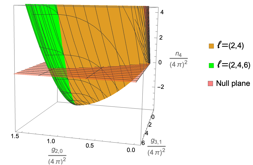
Plotting these surfaces in Figure 26, we observe the null plane first intersects the section corresponding to the sum of spins $(2,4)$ , next the one corresponding to spins $(2,4,6)$ , and so on. This allows us to find the intersection analytically for any such section, since it always contains a sum over a finite number of spins.

To find the intersection of section $(2,4)$ with the null plane we must solve $n_{4}(m_{2},n_{2},m_{3},n_{3})=0$ , with $m_{2}=0$ and $m_{3}$ given by eq.(124). This leads to a degree 8 polynomial in either $n_{2}$ or $n_{3}$ , but only two solutions are real-valued, and only one satisfies $0\leq m_{i},n_{i}\leq 1$ . Plugging this remaining solution into $g_{2,0},g_{3,1}$ we find a boundary shown in Figure 27. This boundary is exact, but only valid until the next section $(2,4,6)$ , whose intersection can be computed in a similar way.

Finally, we can obtain another exact piece of the upper boundary, which corresponds to a contribution given only by the $\ell=0$ moment. We can place it by matching it to the 1D bounds on $g_{2,0}$ and $g_{3,1}$ that we know exactly from eqs.(120) and (121). We obtain

(g_{2,0},g_{3,1}):\ g_{k,q}(m)=A_{k,q}-\frac{L}{k}v_{\ell_{1},k,q}m^{k}\,,

(129)

with $g_{2,0}(1)=g_{2,0}^{\textrm{upper bound}}$ and $g_{3,1}(0)=g_{3,1}^{\textrm{upper bound}}$ , allowing us to fix $A_{k,q}$ .

Putting all the boundaries together, we obtain Figure 27. The remaining gap can be filled by successively adding more and more spins to the 3D space, and intersecting with the null constraint.

Higher order null constraints from LP

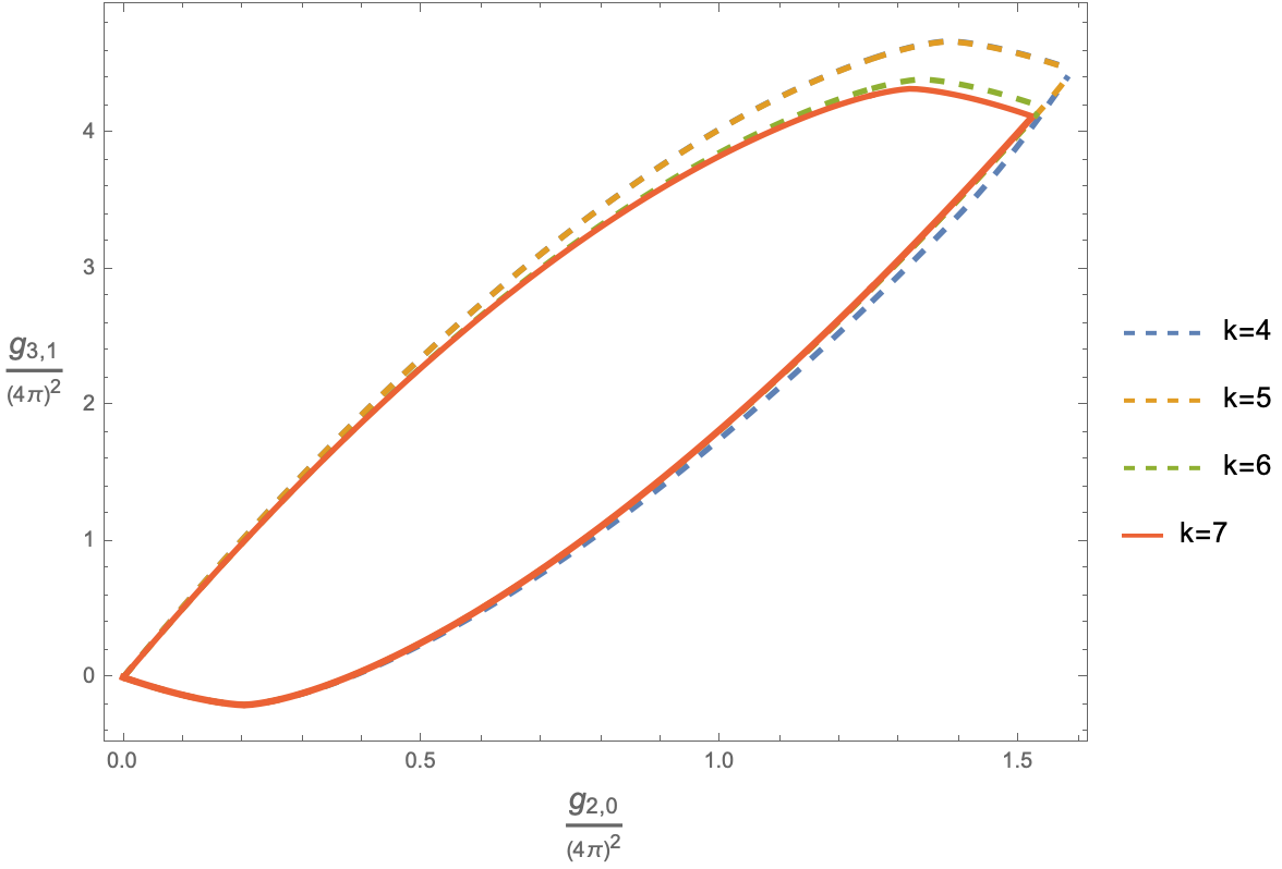
The linear programming setup introduced in Chiang:2022jep allows us to compute the effect of several null constraints. We plot the result including null constraints up to $k=7$ in Figure 28, observing the boundaries already start converging around this order.

4.2.3 Bounds for arbitrary $k$ with $k=4$ null constraint

We can easily derive an upper bound due to the $k=4$ null constraint for any coupling of the form $g_{k,0}$ for $k=even$ , since $\lambda_{\ell,k,0}=2$ , and so the overall boundary structure does not change as we increase $k$ . We must therefore find the boundaries for a space $(n_{4},g_{k,0})$ . We choose this ordering to maintain our convention that $k_{2}\geq k_{1}$ . For any $k$ there will be three types of moments. For $\ell=2$ we have $(-,+)$ , for $\ell=0$ we have $(0,+)$ , and for all the spins $\ell\geq 4$ we have $(+,+)$ . These are shown in Figure 29, together with the boundary structure of their sum. Note that unlike the previous two cases for $g_{2,0}$ and $g_{3,1}$ , the sum of upper boundaries for spins $\ell\geq 4$ no longer gives just a trivial vertical line. Because the slope for each spin is given by $\theta_{\ell}=\frac{v_{\ell,k,0}}{u_{\ell,4}}=\frac{2}{\mathcal{J}^{4}-8\mathcal{J}^{2}}$ , we actually have that largest slope is finite and corresponds to $\ell_{3}$ , with $\theta_{\ell_{3}}\geq\theta_{\ell_{4}}\geq\ldots\geq\theta_{\infty}=0$ . We can therefore use eq.(81) for this boundary.

The Minkowski sum of all boundaries is

	$\displaystyle g_{k,0}(m_{1},m_{2},m_{i})$	$\displaystyle=$	$\displaystyle\frac{L}{k}\left(v_{\ell_{1},k,0}m_{1}^{k}+v_{\ell_{2},k,0}m_{2}^{k}+\sum_{i=3}^{\infty}v_{\ell_{i},k,0}(1-m_{i}^{k})\right)\,,$
	$\displaystyle n_{4}(m_{1},m_{2},m_{i})$	$\displaystyle=$	$\displaystyle\frac{L}{4}\left(u_{\ell_{1},4}m_{1}^{4}+u_{\ell_{2},u}m_{2}^{4}+\sum_{i=3}^{\infty}u_{\ell_{i},4}(1-m_{i}^{4})\right)\,,$		(130)

Arranging the boundaries in order, starting at the origin, the first two sections are given by choosing

	Section 1:		$\displaystyle g_{k,0}(m,0,0),\quad n_{4}(m,0,0)\,,$
	Section 2:		$\displaystyle g_{k,0}(1,m,0),\quad n_{4}(1,m,0)\,.$		(131)

The next two sections are given by

	$\displaystyle\textrm{Section 3: }g_{k,0}$	$\displaystyle=\frac{L}{k}\left(v_{\ell_{2},k,0}+v_{\ell_{1},k,0}+v_{\ell_{3},k,0}(1-m^{k})\right)\,,$
	$\displaystyle n_{4}$	$\displaystyle=\frac{L}{4}\left(u_{\ell_{2},4}+u_{\ell_{1},4}+u_{\ell_{3},u}(1-m^{4})\right)\,,$		(132)

for $m\in[r_{3,4},1]$ and

	$\displaystyle\textrm{Section 4: }g_{k,0}$	$\displaystyle=\frac{L}{k}\left(v_{\ell_{2},k,0}+v_{\ell_{1},k,0}+\left(v_{\ell_{3},k,0}(1-\left(mr_{2,3}\right)^{k})+v_{\ell_{4},k,0}(1-m^{k})\right)\right)\,,$
	$\displaystyle n_{4}$	$\displaystyle=\frac{L}{4}\left(u_{\ell_{2},4}+u_{\ell_{1},4}+\left(u_{\ell_{3},4}(1-\left(mr_{2,3}\right)^{4})+u_{\ell_{4},4}(1-m^{4})\right)\right)\,,$		(133)

for $m\in[r_{4,5},1]$ .

The intersection with the null plane will occur in some section $j\geq 3$ , depending on $k$ . For instance, for $4\leq k\leq 256$ the intersection is in section $j=3$ , while for $258\leq k\leq 1876$ the intersection is in section $j=4$ , and so on, as shown in Figure 29. For $4\leq k\leq 256$ we find an upper bound

\frac{g_{k,0}}{(4\pi)^{2}}\leq\frac{2}{k}\left(30-18\left(\frac{35}{36}\right)^{\frac{k}{4}}\right)\frac{1}{\pi^{2}M^{2k}}\,.

(134)

This upper bound matches that of $g_{4,0}$ in eq.(108) that we found using the polytope constraints, as it must. For $g_{6,0}$ we obtain an upper bound $\sim 0.430$ , stronger than the bound obtained in eq.(112) using the $k=6$ null constraint. This result can be compared to purely projective bounds, which would only imply $g_{k,0}\leq g_{2,0}$ .

For higher $k$ , when the null plane intersects the section $j=4$ , the modification is relatively small. We compare the two in Figure 30. In both cases the bound roughly behaves as $\frac{1}{k}$ , and we expect this behavior to continue for even higher $k$ .

The same derivation can also be similarly carried out for couplings $g_{k,1}$ for $k=odd$ , since these only have a slightly more complicated $\lambda_{\ell,k,q}=2\mathcal{J}^{2}-k$ . We have verified the upper bound follows a similar $1/k$ dropoff, but the lower bound diverges with large $k$ . We can obtain the minimum bound by summing only the negative contributions when $\lambda_{\ell,k,q}<0$ , that is all spins for which $\ell\leq\ell^{*}=1/2(-1+\sqrt{1+2k})\sim\sqrt{k}$ . This gives a lower bound

g_{k,1}\geq\frac{16}{k}\sum_{\ell<\ell^{*}}(2\ell+1)(2(\ell^{2}+\ell)-k)\,.

(135)

For large $k$ this approximates to $-2k$ . Imposing any finite number of null constraints does not affect this bound.

It is interesting to compare this behavior with an example of a physical theory. We can consider a theory with a massive scalar $m_{x}$ , with no tree level interaction, such that the first allowed amplitude is the 1-loop box, given by

	$\displaystyle M(s,t)=\lambda^{4}$	$\displaystyle\int\frac{d^{4}\ell}{(2\pi)^{4}}\frac{1}{\left[\ell^{2}-m_{x}^{2}\right]\left[\left(\ell-p_{1}\right)^{2}-m_{x}^{2}\right]\left[\left(\ell-p_{1}-p_{2}\right)^{2}-m_{x}^{2}\right]\left[\left(\ell+p_{4}\right)^{2}-m_{x}^{2}\right]}$
		$\displaystyle+perm(2,3,4)\,.$		(136)

The low energy expansion can be computed by first writing the integral in Feynman parameterization, which in $D=4$ is

I(s,t)=\int_{0}^{1}da_{i}^{4}\delta(1-\sum_{i}a_{i})\frac{1}{\left(a_{1}a_{3}s+a_{2}a_{4}t+m_{x}^{2}\right)^{2}}\,,

(137)

In terms of the EFT scale $M$ , we have $M=2m_{x}$ , since the lightest state for this process is in fact a two-particle state. Summing over all permutations, we obtain, for $k=\{0,2,4,\ldots\}$ :

\displaystyle g_{k,0}:

\displaystyle\frac{2^{4}\tilde{\lambda}^{4}}{2M^{4}}\left\{1,\frac{2^{4}}{60M^{4}},\frac{2^{8}}{1890m_{x}^{8}},\frac{2^{12}}{48048m_{x}^{12}},\frac{2^{16}}{1093950m_{x}^{16}},\frac{2^{20}}{23279256m_{x}^{20}},\ldots\right\}

We observe these couplings follow a stronger approximately $1/k!$ fall-off. For normalization we match to the upper bound we derived for $g_{4,0}\leq 0.633$ , such that the remaining couplings are consistent with our bound in eq.(134), as shown in Figure 31. Note that at leading orders, the scalar box is close to our numeric bounds which indicate that the bounds are close to optional. The deviation increases at large $k$ .

5 Conclusions

In this paper we developed a non-projective generalization of the EFThedron, allowing us to incorporate the non-linear unitarity bound in full. This allows us to derive non-projective upper bounds for the EFT couplings, which shows that while the leading derivative couplings are of $\mathcal{O}(1)$ , they are heavily suppressed at higher $k$ . As a different application of this framework, we can also incorporate the low spin dominance condition, a property observed to hold for gravitational EFT Bern:2021ppb (see also Figueroa:2022onw). It would also be interesting to explore how to implement the upper bound on $\rho$ for impact parameter space dispersion relations in gravitational EFT Caron-Huot:2022ugt; Caron-Huot:2021rmr.

In Section 2 we solved the single $L$ -moment problem by treating it as a Minkowski sum of segments. To our knowledge this a new proof to this problem. It would be interesting if the same approach could be used to solve the double $L$ -moment problem PUTINAR1990288, and perhaps understand new features of this much richer topic. At the same time, it would be interesting if the known solution to the double $L$ -moment can be used to obtain bounds on our physical problem. This would enable the approach used in the projective case, which is easier to set up and extend to higher dimensional spaces and more null constraints.

Acknowledgements.

L-y Chiang, Y-t Huang, and H-c Weng are supported by Taiwan Ministry of Science and Technology Grant No. 109-2112-M-002 -020 -MY3. L Rodina is supported by Taiwan Ministry of Science and Technology Grant No. 109-2811-M-002-523.

Appendix A Aspects of the $L$ -moment problem

In this section we discuss some other interesting aspects of the $L$ -moment problem, in particular the functions $\rho$ that correspond to our boundary solutions, also known as extremal solutions, and the formulation of constraints in terms of “exponential Hankel” matrices.

A.1 Boundary distributions

The boundary solutions for $a_{k}$ correspond to particular $\rho$ , which we can easily work out. For instance, the boundary of a 2D space we found was given by

a_{k,q}=\int_{0}^{1}\rho z^{k-1}dz=L\frac{m^{k}}{k}\,,

(139)

and we find the corresponding boundary $\rho$ is a step function

\chi_{I}(z)=\left\{\begin{array}[]{ll}L&\textrm{for }z\in I\,,\\ 0&\textrm{for }z\notin I\,.\end{array}\right.

(140)

In general, a solution may contain a sum over several such functions,

\rho(z)=\sum_{i=1}^{N}\chi_{I_{i}}(z)\,,

(141)

where $I_{i}=[m_{2i-1},m_{2i}]$ , $m_{i}\leq m_{i+1}$ . Just like the boundary itself, we can deduce the corresponding distributions directly from eqs.(2.2) and (2.2), depending on dimension, by simply taking ${\bf V}_{i_{1},i_{2}}\rightarrow\chi_{[m_{i_{1}},m_{i_{2}}]}$ . For $D=\textrm{even}$ we find

	$\displaystyle\textrm{lower: }\rho(z)$	$\displaystyle=$	$\displaystyle\chi_{[0,m_{1}]}+\chi_{[m_{2},m_{3}]}+\ldots+\chi_{[{m_{D-2}},m_{D-1}]}\,,$
	$\displaystyle\textrm{upper: }\rho(z)$	$\displaystyle=$	$\displaystyle\chi_{[m_{1},m_{2}]}+\chi_{[m_{3},m_{4}]}+\ldots+\chi_{[{m_{D-1}},1]}\,,$		(142)

and for $D=\textrm{odd}$

	$\displaystyle\textrm{lower: }\rho(z)$	$\displaystyle=$	$\displaystyle\chi_{[m_{1},m_{2}]}+\chi_{[m_{3},m_{4}]}+\ldots+\chi_{[{m_{D-2}},m_{D-1}]}\,,$
	$\displaystyle\textrm{upper: }\rho(z)$	$\displaystyle=$	$\displaystyle\chi_{[0,m_{1}]}+\chi_{[m_{2},m_{3}]}+\ldots+\chi_{[{m_{D-1}},1]}\,.$		(143)

A.2 Exponential Hankel conditions

Similar to the projective moment problem, necessary and sufficient conditions for the $L$ -moments can be expressed in terms of positive semi-definite matrices. Using the notation of PUTINAR1990288, the conditions for the infinite dimensional problem are given in terms of two new sequences, $b$ and $c$ , defined by

	$\displaystyle\textrm{exp}\left[{-\frac{1}{L}\left(\frac{a_{0}}{X}{+}\frac{a_{1}}{X^{2}}{+}\cdots\right)}\right]$	$\displaystyle=$	$\displaystyle 1-\left(\frac{b_{0}}{X}{+}\frac{b_{1}}{X^{2}}{+}\cdots\right)\,,$
	$\displaystyle\textrm{exp}\left[{\frac{1}{L}\left(\frac{a_{0}}{X}{+}\frac{a_{1}}{X^{2}}{+}\cdots\right)}\right]$	$\displaystyle=$	$\displaystyle 1+\left(\frac{c_{0}}{X}{+}\frac{c_{1}}{X^{2}}{+}\cdots\right)\,,$		(144)

which must satisfy the usual Hankel positivity constraints, for all $n$ .

1.

$x\in(-\infty,\infty)$ :

$H_{n}(b)\geq 0\,.$ (145)
2.

$x\in[0,\infty)$ :

$H_{n}(b),\ H_{n}^{\textrm{shift}}(b)\geq 0\,.$ (146)
3.

$x\in[0,1]$ :

$H_{n}(b),\ H_{n}^{\textrm{shift}}(b),\ H_{n}^{\textrm{twist}}(c)\geq 0\,.$ (147)

One can verify that for the boundary solutions we found particular subsets of the exponential Hankels indeed vanish. This implies the Hankel constraints are necessary conditions. Next we review the proof they are also sufficient conditions, in the $x\in(-\infty,\infty)$ case.

Let us begin with the exponential map

e^{\frac{1}{L}\left(\frac{a_{0}}{x}{+}\frac{a_{1}}{x^{2}}{+}\cdots\frac{a_{2m}}{x^{2m{+}1}}\right)}=1{+}\frac{b_{0}}{x}{+}\frac{b_{1}}{x^{2}}{+}\cdots

(148)

Note that while there are $2m$ $a_{i}$ s, the exponential map generates an infinite series for $b_{i}$ s. We would like to show that if the $b_{i}$ satisfy Hankel positivity condition, we can use them to build a solution for the $L$ -moment problem for the $\{a_{i}\}$ s. This applies to the Hamburger, Stieltjes and Hausdorff intervals $\mathcal{I}$ . For a general discussion see akhiezer1962some.

So let us begin by $b_{i}$ being a solution to the Hamburger moment problem. Note that since the LHS of eq.(148) has $2m{+}1$ $\{a_{i}\}$ s, this means that the first $2m{+}1$ $\{b_{i}\}$ s on the RHS should fully determine the $\{a_{i}\}$ s. This further suggests that $b_{2k{+}1},b_{k{+}2},\cdots$ are also fully determined by $\{b_{0},b_{1},\cdots,b_{2m{+}1}\}$ , and thus the $\{b_{i}\}$ s correspond to a solution with $m{+}1$ elements in the hull:

b_{i}=\sum_{a=1}^{m{+}1}\tilde{\rho}_{a}y_{a}^{i},\quad\tilde{\rho}_{a}>0\,.

(149)

Substituting this into the exponential map the RHS can be rewritten as

1{+}\frac{b_{0}}{x}{+}\frac{b_{1}}{x^{2}}{+}\cdots=1{+}\sum_{a=1}^{m{+}1}\frac{\tilde{\rho}_{a}}{x{-}y_{a}}\equiv\frac{\psi(x)}{\phi(x)}\,,

(150)

where

\phi(x)=\prod_{a=1}^{m{+}1}(x{-}y_{a}),\quad\psi(x)=\prod_{a=1}^{m{+}1}(x{-}y^{\prime}_{a})\,,

(151)

and $y^{\prime}_{1}<y_{1}<y_{2}^{\prime}<y_{2}<\cdots<y^{\prime}_{m{+}1}<y_{m{+}1}$ , i.e. the position of zeros for $\psi(x)$ is distributed in between the zeros of $\phi(x)$ . Now consider the following density:

\rho(u)\equiv\frac{L}{2}\left(1{-}\textrm{sign}\frac{\psi(u)}{\phi(u)}\right)\,.

(152)

We see that $\rho(u)$ is either $L$ or $0$ . Since the zeros of $\psi(x)$ and $\phi(x)$ are interspaced, the integration directly gives

\int du\frac{\rho(u)}{x{-}u}=L\left(\int_{y^{\prime}_{1}}^{y_{1}}\frac{du}{x-u}{+}\int_{y^{\prime}_{2}}^{y_{2}}\frac{du}{x-u}{+}\cdots\right)=L\log\frac{\psi(x)}{\phi(x)}\,.

(153)

Now combine eq.(148) with eq.(150), we have

\left(\frac{a_{0}}{x}{+}\frac{a_{1}}{x^{2}}{+}\cdots\frac{a_{2m}}{x^{2m{+}1}}\right)=L\log\frac{\psi(x)}{\phi(x)}=\int du\frac{\rho(u)}{x{-}u}\quad\rightarrow\quad a_{k}=\int du\;\rho(u)u^{k}\,,

(154)

where $\rho(u)$ is defined in eq.(152). Thus we have constructed a solution to the $L$ -moment problem. Note that the solution corresponds to an $m$ -state solution.

Appendix B Discrete solution to the double moment problem

Let us understand the results in Section 3.2 also from the discrete perspective, instead of the Lagrange method. Our task is to find the boundary for the sum of two lower boundaries

a_{k_{1},q_{1}}=\frac{L}{k}v_{\ell_{1},k,q}m_{1}^{k}+\frac{L}{k}v_{\ell_{2},k,q}m_{2}^{k}

(155)

If we imagine discretizing both curves into small segments, we know the resulting boundary will be given by placing the segments in order according to their slope. The slopes of segments from curve 1 range from $[0,\theta_{1}]$ , while those of curve 2 from $[0,\theta_{2}]$ , where $\theta_{\ell}=v_{\ell,k_{2},q_{2}}/v_{\ell,k_{1},q_{1}}$ . We show this in Figure 32. If we assume $\theta_{2}>\theta_{1}$ , then it is clear the sum will have one section from $[0,\theta_{1}]$ formed with segments originating from both, placed in some particular order, and a second section from $[\theta_{1},\theta_{2}]$ with segments just from curve 2, placed in their original order. In the continuous limit this leads to the result found via Lagrange multipliers. We work this out explicitly next.

Let us now consider a sum of an arbitrary number of moments. We assume the $v_{\ell}$ are ordered and non-negative, such that $0<\theta_{\ell_{1}}\leq\theta_{\ell_{2}}\leq\ldots\leq\theta_{\ell_{n}}<\pi/2$ . This implies all spins $\ell_{1},\ldots,\ell_{n}$ have segments with slopes up to $\theta_{1}$ , but only spins $\ell_{2},\ldots,\ell_{n}$ have segments with slopes from $\theta_{1}$ to $\theta_{2}$ , and so on.

The discretized version of the moments, is given by

a_{k,q}^{(\ell)}=v_{\ell,k,q}\int_{0}^{1}\rho(z)z^{k-1}dz\rightarrow\sum_{i=1}^{N_{\ell}}\rho_{\ell,i}v_{\ell,k,q}\frac{i^{k-1}}{N_{\ell}^{k}},\quad 0\leq\rho_{i,\ell}\leq L\,.

(156)

We can view each moment as a Minkowski sum of segments $s_{i}^{(\ell)}$ , defined in the terms of their endpoint obtained when $\rho_{i,\ell}=L$ :

s_{i,k,q}^{(\ell)}=L\,v_{\ell,k,q}\frac{i^{k-1}}{N_{\ell}^{k}}\,,

(157)

with slopes

\theta_{\ell,i}=\theta_{\ell}\frac{i^{\Delta_{k}}}{N^{\Delta_{k}}}\,.

(158)

Note that as $i$ varies from 0 to $N_{\ell}$ the slopes of the segments vary from 0 to $\theta_{\ell}$ . Let us now consider the range $[0,\theta_{1}]$ , where segments from all spins can appear. We wish to discretize all curves into segments $s_{i}^{(\ell)}$ with equal slope for all $\ell$ . We can achieve this by tuning $N_{\ell}$ for each spin. To obtain segments of equal slope at equal $i$ but different $\ell$ , we require

\theta_{\ell_{1},i}=\theta_{\ell_{2},i}\Rightarrow\frac{N_{1}}{N_{2}}=\left(\frac{\theta_{1}}{\theta_{2}}\right)^{\frac{1}{\Delta_{k}}}=r_{2,1}\,.

(159)

This means each spin must be discretized in a total of $N_{\ell_{i}}=N_{1}/r_{i,1}\geq N_{1}$ segments. The factor $r_{i,1}$ is finite for $\ell\neq 0$ , so the continuous limit remains consistent. For a given spin $\ell_{j}$ we obtain a set of $N_{1}$ segments

s_{i,k,q}^{(\ell_{j})}=L\frac{i^{k}}{N_{1}^{k}}\ell_{j}^{q}r_{j,1}^{k},\quad i\in[0,N_{1}]\,,

(160)

with slopes

\theta_{\ell_{j},i}=\theta_{\ell_{1},i}=\theta_{1}\frac{i^{\Delta_{k}}}{N_{1}^{\Delta_{k}}}\,,

(161)

which unlike eq.(158) are now independent of spin, but still depend on $i$ as they vary from 0 to $\theta_{1}$ . We can now compute the Minkowski sum at fixed $i$ over all spins, since the sum of segments of equal slope simply amounts to another segment of the same slope, with endpoint

S_{i,k,q}^{(1)}=\sum_{\ell}s_{i,k,q}^{(\ell)}=\frac{i^{k}}{N_{1}^{k}}F_{k,q}\,,

(162)

where

F_{k,q}=\sum_{i=1}v_{\ell,k,q}r_{i,j}^{k}\,.

(163)

Crucially, the new segments $S_{i}$ are now ordered according to $i\in[0,N_{1}]$ , as their slope increases monotonically with $i$ , from 0 to $\theta_{1}$ . Next, we can repeat the argument for the range $[\theta_{1},\theta_{2}]$ , and we obtain a new set of vectors $S_{i,k,q}^{(2)}$ , also ordered by $i$ . Taking the union of ${S}^{(1)}$ and ${S}^{(2)}$ we therefore obtain a set of segments ordered by $i\in[N_{1},N_{2}]$ , and so the boundaries of their Minkowksi sum can be obtained from using the results in Section 2. For $j\in[0,N_{1}]$ , corresponding to the range, $[0,\theta_{1}]$ we obtain a vertex on the boundary given by

V_{j|k,q}=\sum_{i=1}^{j}\frac{i^{k}}{N_{1}^{k}}F_{k,q}\,.

(164)

In the continuous limit this becomes

\displaystyle a_{k,q}

\displaystyle=

\displaystyle\frac{L}{k}m^{k}F_{k,q}\,,

(165)

matching what we found using the Lagrange method in eq.(77).

Appendix C Towards a solution for the complete space

In this section we present some partial results on determining the complete space for the simpler “power” moment problem

a_{k,q}=\sum_{\ell}\Lambda_{\ell,q}\int_{0}^{1}\rho_{\ell}(z)z^{k-1}dz\,,

(166)

where $\Lambda_{\ell,q}=g(\ell)f(\ell)^{q}$ , with $g$ and $f$ any positive polynomials in $\ell$ .

C.1 Diagonal spaces

Let us first consider 3D spaces of the form $a_{k_{1},q_{1}},a_{k_{2},q_{2}},a_{k_{3},q_{3}},$ , where the set of $\{k_{i},q_{i}\}$ s satisfy

k_{i+1}-k_{i}=\Delta_{k},\quad q_{i+1}-q_{i}=\Delta_{q}\,,

(167)

For two spins, the Minkowski sum of lower and upper boundaries of this space is given by

	$\displaystyle a_{k,q}$	$\displaystyle=$	$\displaystyle\frac{L}{k}\sum_{\ell}\Lambda_{\ell,q}\left(m_{1}^{(\ell)}-m_{2}^{(\ell)}\right)\,,$
	$\displaystyle\overline{a}_{k,q}$	$\displaystyle=$	$\displaystyle\frac{L}{k}\sum_{\ell}\Lambda_{\ell,q}\left(1-m_{1}^{(\ell)}+m_{2}^{(\ell)}\right)\,,$		(168)

for $1\geq m_{1}^{(\ell)}\geq m_{2}^{(\ell)}\geq 0$ . We must compute the boundary of the Minkowski sum of these boundaries, which is again easily accomplished by the Lagrange multiplier method, also keeping in mind to check the boundaries of parametric space.

For such case, applying the Lagrange method we find:

\frac{m_{1}^{(\ell_{i})}}{m_{1}^{(\ell_{j})}}=\frac{m_{2}^{(\ell_{i})}}{m_{2}^{(\ell_{j})}}=r_{j,i}=\left(\frac{f(\ell_{i})}{f(\ell_{j})}\right)^{\frac{\Delta_{q}}{\Delta_{k}}}\,.

(169)

This reduces the Minkowski sum to just two independent parameters, as required to span the $2$ dimensional boundary. Expressing for instance all parameters as $m_{i}^{(\ell_{j})}=m_{i}^{(\ell_{1})}r_{j,1}=m_{i}r_{j,1}$ , the lower boundary is given by

a_{k,q}=\frac{L}{k}\left((m_{1})^{k}-(m_{2})^{k}\right)\sum_{i}\Lambda_{\ell,q}r_{i,1}^{k}\,.

(170)

which is valid for $1\geq m_{1}\geq m_{2}\geq 0$ , and similarly for the upper boundary. The sum over infinite spins is now separate from the parameters, and so can be evaluated numerically. In higher dimensions, the sum of boundaries is given by

	$\displaystyle a_{k,q}$	$\displaystyle=$	$\displaystyle\frac{L}{k}\sum_{\ell}\Lambda_{\ell,q}\sum_{j=1}^{D-1}(-1)^{j+1}m_{j}^{(\ell)}\,,$
	$\displaystyle\overline{a}_{k,q}$	$\displaystyle=$	$\displaystyle\frac{L}{k}\sum_{\ell}\Lambda_{\ell,q}\left(1-\sum_{j=1}^{D-1}(-1)^{j+1}m_{j}^{(\ell)}\right)\,.$		(171)

Remarkably, the result eq.(169) holds in fact in any number of dimensions, as long as the conditions (167) are satisfied, so it can be plugged in eq.(C.1) to obtain the $D{-}1$ dimensional boundaries.

Finally we need to consider bounds of the parameter space. These will give new boundaries, which as before, can be simply deduced by imposing the upper integration limit as

m_{i}^{\ell_{j}}\rightarrow\textrm{min}[m_{i}^{(\ell_{j})},1]\,.

(172)

Explicitly, the boundary of a $D$ -dimensional space will be labeled by $D-1$ indices $(i_{1},i_{2},\ldots,i_{D-1})$ , with $N\geq i_{1}\geq i_{2}\geq\ldots\geq i_{D-1}\geq 1$ . A value $i_{j}=n$ indicates $m_{j}^{\ell_{i<n}}=1$ and $m_{j}^{\ell_{i\geq n}}=r_{i,n}m_{j}$ , with $m_{j}\in[r_{n,n-1},1]$ .

C.2 Approach to more general spaces

Here we introduce a tentative approach to obtain constraints on the complete space of couplings $a_{k,q}$ . This is motivated by the previous solution to the projective moment problem discussed in Chiang:2021ziz. Recall that a sequence $a_{k}$ can be expressed as a single moment

a_{k}=\int_{\mathbb{R}}\rho(x)x^{k-1},\quad\rho\geq 0\,,

(173)

if and only if the Hankel matrix is totally positive,

H=\begin{pmatrix}a_{1}&a_{2}&a_{3}&\ldots\\ a_{2}&a_{3}\\ \vdots\end{pmatrix}\geq 0\,.

(174)

For double moments,

a_{k,q}=\int_{\mathbb{R}^{2}}\rho(x,y)x^{k-1}y^{q-1},\quad\rho\geq 0\,,

(175)

the conditions are given by total positivity of the moment matrix

M=\begin{pmatrix}a_{1,1}&a_{2,1}&a_{1,2}&a_{3,1}&a_{2,2}&\ldots\\ a_{2,1}&a_{3,1}&a_{2,2}\\ a_{1,2}&a_{2,2}\\ \vdots\end{pmatrix}\geq 0\,.

(176)

There is in fact a simple way to derive the moment matrix from the Hankel matrix. This can be done by considering linear combinations of the double moments that can be written as single moments. For instance we can define

$\displaystyle b_{1}$	$\displaystyle\equiv$	$\displaystyle a_{1,1}=\int\rho\left(x+\gamma xy\right)^{0}\,,$
$\displaystyle b_{2}$	$\displaystyle\equiv$	$\displaystyle a_{2,1}+\gamma a_{2,2}=\int\rho\left(x+\gamma xy\right)^{1}\,,$
$\displaystyle b_{3}$	$\displaystyle\equiv$	$\displaystyle a_{3,1}+2\gamma a_{3,2}+\gamma^{2}a_{3,3}=\int\rho\left(x+\gamma xy\right)^{2}\,,$	(177)

where $\gamma$ is some parameter. Importantly, the new couplings $b_{k}$ are again a sum of single moments $b_{k}=\int\rho z^{k}$ , with $z=x+\gamma xy$ . Thus $b_{k}$ satisfy Hankel conditions, leading to constraints back on the $a_{k,q}$ , such as

H=\begin{pmatrix}b_{1}&b_{2}\\ b_{2}&b_{3}\end{pmatrix}=\begin{pmatrix}a_{1,1}&a_{2,1}+\gamma a_{2,2}\\ a_{2,1}+\gamma a_{2,2}&a_{3,1}+2\gamma a_{3,2}+\gamma^{2}a_{3,3}\end{pmatrix}\geq 0\,.

(178)

Importantly, the above condition now must hold for all values of $\gamma$ . Imposing this through the discriminant equation on the determinant, we recover exactly the same condition as from the $3\times 3$ moment matrix in eq.(176). We have therefore derived the double moment conditions by taking an envelope, parameterized by $\gamma$ , of the single moment conditions.

Let us now attempt to do the same for the double $L$ -moment problem

a_{k,q}=\sum\ell^{q}\int\rho(z)z^{k-1}dx\,.

(179)

We mirror the argument above, by taking linear combinations

$\displaystyle b_{1,1}$	$\displaystyle=$	$\displaystyle a_{1,1}=\sum\int\rho(z)(z+\gamma z\ell)^{0}\,,$
$\displaystyle b_{2,2}$	$\displaystyle=$	$\displaystyle a_{2,1}+\gamma a_{2,2}=\sum\int\rho(z)(z+\gamma z\ell)^{1}\,,$
$\displaystyle b_{3,3}$	$\displaystyle=$	$\displaystyle a_{3,1}+2\gamma a_{3,2}+\gamma^{2}a_{3,3}=\sum\int\rho(z)(z+\gamma z\ell)^{2}\,,$	(180)

and so on, for $\gamma>0$ . We have shown that diagonal spaces with $v_{\ell,k,q}=g(\ell)f(\ell)^{q}$ satisfy simple boundary equations, and in the case above we simply have $v_{\ell,k,q}=(\ell+\gamma)^{q}$ . The boundary (for the first section) is therefore

b_{k,k}=\frac{L}{k}(n^{k}-m^{k})\sum_{\ell}v_{\ell_{i},k,q}r_{i,1}^{k}\,,

(181)

where

r_{i,1}=\left(\frac{\ell_{1}+\gamma}{\ell+\gamma}\right)^{\frac{\Delta q}{\Delta k}}\,.

(182)

The boundary is now a function of the parameter $\gamma$ , and if the analogy with the projective problem is valid, then we expect that taking the intersection of all constraints for all values of $\gamma$ should give necessary and sufficient conditions on the $a_{k,q}$ moments. Unfortunately, it seems unlikely a closed form can be found, since $\gamma$ enters the constraints through the infinite sum in eq.(181), which is no longer a purely numerical factor. One can instead simply numerically compute the envelope (for $\gamma>0$ ). It would also be interesting to consider taking the continuous limit of the discrete sum. In that case the sum becomes a trivial integral, and it may be possible to obtain constraints relevant to the double continuous $L$ -moment problem.

Appendix D Low spin dominance

The solution for the non-projective polytope derived in Section 2 can also be utilized to explore the consequence of low spin dominance (LSD), first discussed in Bern:2021ppb. We begin with the dispersive representation for the couplings

a_{k,q}=\sum_{\ell}v_{\ell,k,q}\int_{0}^{1}\rho_{\ell}(z)z^{k-1}dz,\quad\rho_{\ell}(z)\geq 0\,,

(183)

and consider the mass averaged distribution

\langle\rho_{\ell}\rangle_{k}\equiv\int_{0}^{1}\rho_{\ell}(z)z^{k-1}dz\,.

(184)

The LSD condition is the requirement that

\langle\rho_{\ell_{1}}\rangle_{k}\geq\alpha\langle\rho_{\ell}\rangle_{k}\,,

(185)

where $\ell_{1}$ is the lowest spin in the spectrum, and $\alpha\geq 0$ is some parameter specifying the strength of the the LSD condition. Since for now we only discuss equal $k$ spaces, we will drop the $k$ subscript for simplicity. Separating out the lowest spin, we can write

a_{q}=\sum_{\ell}\langle\rho_{\ell}\rangle v_{\ell,q}=\langle\rho_{\ell_{1}}\rangle v_{\ell,q}+\sum_{\ell>\ell_{1}}\langle\rho_{\ell}\rangle v_{\ell,q}\,.

(186)

We now introduce couplings $\mu_{q}$ ,

\mu_{q}=\sum_{\ell>\ell_{1}}\langle\rho_{\ell}\rangle v_{\ell,q}\,.

(187)

which due to the LSD condition must satisfy $\langle\rho_{\ell_{1}}\rangle\geq\alpha\langle\rho_{\ell}\rangle$ , ie. they satisfy an $L$ -moment problem with $\langle\rho_{\ell}\rangle\leq L=\frac{\langle\rho_{\ell_{1}}\rangle}{\alpha}$ , which through eq.(186) will impose constraints back on $a_{q}$ . Since we are at equal $k$ space, the solution to this problem is given by the polytope conditions in Section 2. Therefore to obtain bounds on the $a_{q}$ couplings, we merely solve for the $\mu_{q}$ in terms of $a_{q}$

\mu_{q}=a_{q}{-}\langle\rho_{\ell_{1}}\rangle v_{\ell_{1},q}\,,

(188)

and impose the polytope constraints in eq.(2.2) on the $\mu_{q}$

P_{I}(\mu_{q}),\ \overline{P}_{I}(\mu_{q})\geq 0\,,

(189)

setting $L=\frac{\langle\rho_{\ell_{1}}\rangle}{\alpha}$ . Unlike the previous problem, here the upper bound $L=\frac{\langle\rho_{\ell_{1}}\rangle}{\alpha}$ is not fixed beforehand, since $\langle\rho_{\ell_{1}}\rangle$ is not known. However, we can demand eq.(189) to hold for any allowed values of $\langle\rho_{\ell_{1}}\rangle$ , and this will still generate constraints. When considering purely projective bounds, this means we simply project out $\langle\rho_{\ell_{1}}\rangle\geq 0$ , leading to optimal constraints on $a_{q}$ purely in terms of $\alpha$ . We can also implement the unitarity bound $\rho\leq 2$ , which implies $\langle\rho_{\ell}\rangle_{k}\leq\frac{2}{k}$ , by instead projecting out $0\leq\langle\rho_{\ell_{1}}\rangle_{k}\leq\frac{2}{k}$ .

References

(1) S. Rychkov, EPFL Lectures on Conformal Field Theory in D $>$ = 3 Dimensions. SpringerBriefs in Physics. 1, 2016. 10.1007/978-3-319-43626-5.
(2) D. Simmons-Duffin, The Conformal Bootstrap, in Theoretical Advanced Study Institute in Elementary Particle Physics: New Frontiers in Fields and Strings, pp. 1–74, 2017. 1602.07982. DOI.
(3) D. Poland, S. Rychkov and A. Vichi, The Conformal Bootstrap: Theory, Numerical Techniques, and Applications, Rev. Mod. Phys. 91 (2019) 015002, [1805.04405].
(4) D. Poland and D. Simmons-Duffin, Snowmass White Paper: The Numerical Conformal Bootstrap, in 2022 Snowmass Summer Study, 3, 2022. 2203.08117.
(5) F. Caracciolo and V. S. Rychkov, Rigorous Limits on the Interaction Strength in Quantum Field Theory, Phys. Rev. D 81 (2010) 085037, [0912.2726].
(6) A. Manohar and H. Georgi, Chiral Quarks and the Nonrelativistic Quark Model, Nucl. Phys. B 234 (1984) 189–212.
(7) S. Caron-Huot and V. Van Duong, Extremal Effective Field Theories, JHEP 05 (2021) 280, [2011.02957].
(8) A. Adams, N. Arkani-Hamed, S. Dubovsky, A. Nicolis and R. Rattazzi, Causality, analyticity and an IR obstruction to UV completion, JHEP 10 (2006) 014, [hep-th/0602178].
(9) T. N. Pham and T. N. Truong, Evaluation of the Derivative Quartic Terms of the Meson Chiral Lagrangian From Forward Dispersion Relation, Phys. Rev. D 31 (1985) 3027.
(10) B. Ananthanarayan, D. Toublan and G. Wanders, Consistency of the chiral pion pion scattering amplitudes with axiomatic constraints, Phys. Rev. D 51 (1995) 1093–1100, [hep-ph/9410302].
(11) B. Bellazzini, L. Martucci and R. Torre, Symmetries, Sum Rules and Constraints on Effective Field Theories, JHEP 09 (2014) 100, [1405.2960].
(12) B. Bellazzini, Softness and amplitudes’ positivity for spinning particles, JHEP 02 (2017) 034, [1605.06111].
(13) C. de Rham, S. Melville, A. J. Tolley and S.-Y. Zhou, Positivity bounds for scalar field theories, Phys. Rev. D 96 (2017) 081702, [1702.06134].
(14) C. de Rham, S. Melville, A. J. Tolley and S.-Y. Zhou, UV complete me: Positivity Bounds for Particles with Spin, JHEP 03 (2018) 011, [1706.02712].
(15) C. de Rham, S. Melville, A. J. Tolley and S.-Y. Zhou, Positivity Bounds for Massive Spin-1 and Spin-2 Fields, JHEP 03 (2019) 182, [1804.10624].
(16) B. Bellazzini, F. Riva, J. Serra and F. Sgarlata, Massive Higher Spins: Effective Theory and Consistency, JHEP 10 (2019) 189, [1903.08664].
(17) L. Alberte, C. de Rham, A. Momeni, J. Rumbutis and A. J. Tolley, Positivity Constraints on Interacting Pseudo-Linear Spin-2 Fields, JHEP 07 (2020) 121, [1912.10018].
(18) B. Bellazzini, J. Elias Miró, R. Rattazzi, M. Riembau and F. Riva, Positive moments for scattering amplitudes, Phys. Rev. D 104 (2021) 036006, [2011.00037].
(19) A. J. Tolley, Z.-Y. Wang and S.-Y. Zhou, New positivity bounds from full crossing symmetry, JHEP 05 (2021) 255, [2011.02400].
(20) N. Arkani-Hamed, T.-C. Huang and Y.-T. Huang, The EFT-Hedron, JHEP 05 (2021) 259, [2012.15849].
(21) M. B. Green and C. Wen, Superstring amplitudes, unitarily, and Hankel determinants of multiple zeta values, JHEP 11 (2019) 079, [1908.08426].
(22) Y.-t. Huang, J.-Y. Liu, L. Rodina and Y. Wang, Carving out the Space of Open-String S-matrix, JHEP 04 (2021) 195, [2008.02293].
(23) A. Sinha and A. Zahed, Crossing Symmetric Dispersion Relations in Quantum Field Theories, Phys. Rev. Lett. 126 (2021) 181601, [2012.04877].
(24) Z.-Y. Wang, C. Zhang and S.-Y. Zhou, Generalized elastic positivity bounds on interacting massive spin-2 theories, JHEP 04 (2021) 217, [2011.05190].
(25) T. Trott, Causality, unitarity and symmetry in effective field theory, JHEP 07 (2021) 143, [2011.10058].
(26) Y.-J. Wang, F.-K. Guo, C. Zhang and S.-Y. Zhou, Generalized positivity bounds on chiral perturbation theory, JHEP 07 (2020) 214, [2004.03992].
(27) A. Hebbar, D. Karateev and J. Penedones, Spinning S-matrix Bootstrap in 4d, 2011.11708.
(28) J. Elias Miró and A. Guerrieri, Dual EFT bootstrap: QCD flux tubes, JHEP 10 (2021) 126, [2106.07957].
(29) L. Alberte, C. de Rham, S. Jaitly and A. J. Tolley, Reverse Bootstrapping: IR lessons for UV physics, 2111.09226.
(30) S. D. Chowdhury, K. Ghosh, P. Haldar, P. Raman and A. Sinha, Crossing Symmetric Spinning S-matrix Bootstrap: EFT bounds, 2112.11755.
(31) P. Raman and A. Sinha, QFT, EFT and GFT, JHEP 12 (2021) 203, [2107.06559].
(32) P. Haldar, A. Sinha and A. Zahed, Quantum field theory and the Bieberbach conjecture, SciPost Phys. 11 (2021) 002, [2103.12108].
(33) A. Zahed, Positivity and geometric function theory constraints on pion scattering, JHEP 12 (2021) 036, [2108.10355].
(34) Z.-Z. Du, C. Zhang and S.-Y. Zhou, Triple crossing positivity bounds for multi-field theories, JHEP 12 (2021) 115, [2111.01169].
(35) X. Li, H. Xu, C. Yang, C. Zhang and S.-Y. Zhou, Positivity in Multifield Effective Field Theories, Phys. Rev. Lett. 127 (2021) 121601, [2101.01191].
(36) C. Zhang, SMEFTs living on the edge: determining the UV theories from positivity and extremality, 2112.11665.
(37) J. Albert and L. Rastelli, Bootstrapping Pions at Large $N$ , 2203.11950.
(38) Z. Bern, D. Kosmopoulos and A. Zhiboedov, Gravitational effective field theory islands, low-spin dominance, and the four-graviton amplitude, J. Phys. A 54 (2021) 344002, [2103.12728].
(39) J. Henriksson, B. McPeak, F. Russo and A. Vichi, Rigorous Bounds on Light-by-Light Scattering, 2107.13009.
(40) J. Davighi, S. Melville and T. You, Natural selection rules: new positivity bounds for massive spinning particles, JHEP 02 (2022) 167, [2108.06334].
(41) S. Melville and J. Noller, Positivity bounds from multiple vacua and their cosmological consequences, 2202.01222.
(42) S. Caron-Huot, D. Mazac, L. Rastelli and D. Simmons-Duffin, Sharp boundaries for the swampland, JHEP 07 (2021) 110, [2102.08951].
(43) S. Caron-Huot, Y.-Z. Li, J. Parra-Martinez and D. Simmons-Duffin, Causality constraints on corrections to Einstein gravity, 2201.06602.
(44) J. Henriksson, B. McPeak, F. Russo and A. Vichi, Bounding Violations of the Weak Gravity Conjecture, 2203.08164.
(45) K. Häring and A. Zhiboedov, Gravitational Regge bounds, 2202.08280.
(46) M. Kruczenski, J. Penedones and B. C. van Rees, Snowmass White Paper: S-matrix Bootstrap, 2203.02421.
(47) C. de Rham, S. Kundu, M. Reece, A. J. Tolley and S.-Y. Zhou, Snowmass White Paper: UV Constraints on IR Physics, in 2022 Snowmass Summer Study, 3, 2022. 2203.06805.
(48) M. Correia, A. Sever and A. Zhiboedov, An Analytical Toolkit for the S-matrix Bootstrap, 2006.08221.
(49) B. Bellazzini, M. Riembau and F. Riva, The IR-Side of Positivity Bounds, 2112.12561.
(50) D. Simmons-Duffin, A Semidefinite Program Solver for the Conformal Bootstrap, JHEP 06 (2015) 174, [1502.02033].
(51) W. Landry and D. Simmons-Duffin, Scaling the semidefinite program solver SDPB, 1909.09745.
(52) L.-Y. Chiang, Y.-t. Huang, W. Li, L. Rodina and H.-C. Weng, Into the EFThedron and UV constraints from IR consistency, 2105.02862.
(53) A. Guerrieri, J. Penedones and P. Vieira, Where Is String Theory in the Space of Scattering Amplitudes?, Phys. Rev. Lett. 127 (2021) 081601, [2102.02847].
(54) F. Figueroa and P. Tourkine, On the unitarity and low energy expansion of the Coon amplitude, 2201.12331.
(55) L.-Y. Chiang, Y.-t. Huang, W. Li, L. Rodina and H.-C. Weng, (Non)-projective bounds on gravitational EFT, 2201.07177.
(56) E. Herrmann and J. Trnka, The SAGEX Review on Scattering Amplitudes, Chapter 7: Positive Geometry of Scattering Amplitudes, 2203.13018.
(57) F. Hausdorff, Momentprobleme für ein endliches intervall., Mathematische Zeitschrift 16 (1923) 220–248.
(58) M. G. Krein, D. Louvish and A. A. Nudelman, The markov moment problem and extremal problems, 1977.
(59) M. Putinar, The l problem of moments in two dimensions, Journal of Functional Analysis 94 (1990) 288–307.
(60) D. Freedman and P. Diaconis, The markov moment problem and de finetti?s theorem: Part i, Mathematische Zeitschrift 247 (05, 2004) 183–199.
(61) N. Akhiezer and M. Krein, Über fouriersche reihen beschränkter summierbarer funktionen und ein neues extremumproblem, Common. Soc. Math., Kharkov 9 (1934) .
(62) N. I. Akhiezer and W. Fleming, Some questions in the theory of moments, vol. 2. American Mathematical Soc., 1962.

De-projecting the EFThedron

Abstract

1 Introduction

2 De-projection of convex hulls

2.1 Minkowski sums

2.2 De-projecting the cyclic polytope

Two dimensions

3D

General dimension

Non-cyclic vectors

2.3 De-projecting the moment problem: The LL-moment

3 Minkowski sums of single LL-moments

3.1 Extremizing the Minkowski sum

3.2 Two dimensions with k1≠k2k_{1}{\neq}k_{2}

Convergence for infinite spin limit

Non-positive vℓ,k,qv_{\ell,k,q}

3.3 Higher dimensional spaces

4 The non-projective EFThedron

4.1 Bounding gk,qg_{k,q} with kk-null constraint

k=4k=4 bounds

k=5k=5 bounds

k=6k=6 bounds

4.2 Bounding gk1,qg_{k_{1},q} with k≠k1k{\neq}k_{1}-null constraint

4.2.1 Bounds on g2,0g_{2,0}, g3,1g_{3,1} with k=4k{=}4-null constraint

1D bounds on g2,0g_{2,0}

1D bounds on g3,1g_{3,1}

4.2.2 2D theory space for (g2,0,g3,1)(g_{2,0},g_{3,1}) with k=4k{=}4-null constraint

Lower boundary

Upper boundary

Higher order null constraints from LP

4.2.3 Bounds for arbitrary kk with k=4k=4 null constraint

5 Conclusions

Acknowledgements.

Appendix A Aspects of the LL-moment problem

A.1 Boundary distributions

A.2 Exponential Hankel conditions

Appendix B Discrete solution to the double moment problem

Appendix C Towards a solution for the complete space

C.1 Diagonal spaces

C.2 Approach to more general spaces

Appendix D Low spin dominance

References

2.3 De-projecting the moment problem: The $L$ -moment

3 Minkowski sums of single $L$ -moments

3.2 Two dimensions with $k_{1}{\neq}k_{2}$

Non-positive $v_{\ell,k,q}$

4.1 Bounding $g_{k,q}$ with $k$ -null constraint

$k=4$ bounds

$k=5$ bounds

$k=6$ bounds

4.2 Bounding $g_{k_{1},q}$ with $k{\neq}k_{1}$ -null constraint

4.2.1 Bounds on $g_{2,0}$ , $g_{3,1}$ with $k{=}4$ -null constraint

1D bounds on $g_{2,0}$

1D bounds on $g_{3,1}$

4.2.2 2D theory space for $(g_{2,0},g_{3,1})$ with $k{=}4$ -null constraint

4.2.3 Bounds for arbitrary $k$ with $k=4$ null constraint

Appendix A Aspects of the $L$ -moment problem