Local interpretation of time-resolved X-ray absorption in Mott insulators:
Insights from nonequilibrium dynamical mean-field theory
Abstract
We present a formalism based on nonequilibrium dynamical mean field theory (DMFT) which allows to compute the time-resolved X-ray absorption spectrum (XAS) of photo-excited solids. By applying this formalism to the photo-doped half-filled and quarter-filled two-orbital Hubbard models in the Mott insulating regime we clarify how the time-resolved XAS signal reflects the nonequilibrium population of different local states. Apart from the missing broadening associated with continuum excitations, the atomic XAS spectrum computed with the nonthermal state populations provides a good approximation to the full nonequilibrium DMFT result. This suggest a route to combine the accurate DMFT description of nonequilibrum states of solids with cluster calculations of the XAS signal.
I Introduction
X-ray absorption spectroscopy (XAS) allows to explore the local electronic configuration in solids. It is element-specific and has a sufficiently high energy resolution to distinguish different valence states of a given atom. Together with the charge conserving nature of the probe, this makes XAS an attractive technique for the study of Mott insulators and correlated materials.van der Laan et al. 1986; Himpsel et al. 1991; Haverkort et al. 2004 XAS is particularly appealing for the investigation of photo-excited nonequilibrium states,Basov et al. 2017; Giannetti et al. 2016; de la Torre et al. 2021 since new generation free-electron laser sources enable time-resolved XAS (trXAS) measurements with high energy resolution,Baykusheva et al. 2022 and provide information on the nonequilibrium electronic structure which is complementary to time-resolved photoemission. Since the X-ray absorption process represents the first step in resonant inelastic X-ray scattering (RIXS) experiments, a better understanding of trXAS is also relevant in the context of time-resolved RIXS, which can reveal the nonequilibrium physics of low-energy excitations.Mitrano and Wang 2020
XAS on correlated materials can often be well understood in a local picture, because its final state typically involves strongly bound excitons formed by the localized core hole and the valence electrons. The spectra can therefore be described to a good approximation using small clusters obtained within ligand field theory,Haverkort et al. 2012 which gives access to local properties such as multiplet energies, crystal-field excitations, etc. In a photo-excited system out of equilibrium, we expect that fundamental dynamical processes will be reflected in these local properties. For example, the redistribution of charges between different orbitals will modify the screening of local interactions (Hubbard ) and change the electrostatic interaction between the orbitals (Hartree band shifts). This can give rise to level shiftsWegkamp et al. 2014; Golež et al. 2019; Tancogne-Dejean et al. 2018 which should be directly reflected in the XAS signal.Baykusheva et al. 2022 In multi-orbital systems we furthermore expect an ultrafast change of local multiplet occupations. For example, in a degenerate two-orbital Mott insulator at half-filling, the dominant local multiplet in equilibrium is the high-spin state, but after a laser excitation the photo-doped carriers can assist the ultrafast creation of other multiplets (so called Hund’s excitons, i.e., inter- and intra-orbital singlets) which can be relatively long lived.Strand et al. 2017; Rincón et al. 2018; Petocchi et al. 2019; Gillmeister et al. 2020
Due to its local nature, trXAS would be ideal to reveal these ultrafast local processes, which are likely to influence also photo-induced phase transitions and hidden phases. Yet, it is not straightforward to adapt the conventional cluster interpretation of XAS to the time-domain. Even if one can define a finite cluster that captures the dynamics of a local exciton, there is no simple principle which defines the nonequilibrium initial state of this cluster before the X-ray absorption, in contrast to equilibrium, where the initial state is the cluster ground state. A pragmatic approach would be to use a small cluster (maybe even a single atom) with renormalized parameters and with an adjustable initial quantum state to compute the spectrum and then determine the actual time-dependent configuration by comparison to the experimental spectrum at a given probe time. Such an approach would, however, need to be supported by theory.
In equilibrium, dynamical mean-field theory (DMFT)Georges et al. 1996 provides a strategy to construct an optimal embedded cluster model: DMFT maps the correlated lattice problem onto an Anderson impurity model, which can directly be used to compute X-ray spectroscopy signals.Cornaglia and Georges 2007 In particular, the combination of ab-initio input from density-functional theory with DMFT has enabled material-specific calculations for both XAS and RIXS.Haverkort et al. 2014; Lüder et al. 2017; Hariki et al. 2018; Hariki et al. 2020; Higashi et al. 2021 Along the same lines, nonequilibrium DMFT Aoki et al. 2014 simulations directly provide a suitable nonequilibrium impurity problem from which X-ray spectroscopies can be calculated. This approach has been used recently to compute time-resolved RIXS within nonequilibrium DMFT Eckstein and Werner 2021 for photo-doped Hubbard models and electron-phonon coupled systems.Werner et al. 2021; Werner and Eckstein 2021 In these simulations, a nonequilibrium impurity-problem with a self-consistently determined DMFT bath is coupled to a core level. The core-valence excitation by the X-ray pulse is then obtained from time-dependent response functions analogous to what would have to be computed in exact diagonalization studies, Chen et al. 2019; Wang et al. 2020 but for the continuous environment.
In this paper, we discuss how the DMFT approach can be used to compute the trXAS signal, focusing on the half-filled and quarter-filled two-band Mott insulator as a representative example. The explicit time-dependent numerical calculations support the simpler above-mentioned interpretation based on few-site or atomic clusters in combination with nonequilibrium initial states, i.e., the atomic XAS signals computed with the non-thermal populations of the time-evolving state provide a good approximation of the nonequilibrium DMFT result. trXAS therefore allows to track the nonequilibrium populations of the local many-body states. In addition, a change of the line broadening out of equilibrium can be related to additional decay channels for the excitonic final states, which are activated by photo-excitation.
The paper is organized as follows: In Sec. II we present the general formalism and the observables needed to calculate the time-dependent XAS signal. This section is closely related to the formalism derived in the context of RIXS in Ref. Eckstein and Werner 2021, but adapted here to the measurement of the XAS signal. Section III presents the applications of the nonequilibrium DMFT-based XAS formalism to the photo-excited half-filled and quarter-filled two-orbital Hubbard model, and the analysis of the time-dependent spectra. Section IV contains a summary and conclusions.
II Formalism
II.1 General remarks
As in the equilibrium DMFT schemes for calculating X-ray scattering and absorptionHaverkort et al. 2014; Lüder et al. 2017; Hariki et al. 2018; Hariki et al. 2020 a core level is added to the DMFT impurity model, and the spectra are computed for a fixed hybridization function. The trXAS simulation thus involves two steps: (i) A nonequilibrium DMFT simulation determines the time-dependent valence band hybridization function which represents the pump-induced nonequilibrium state of the lattice system, and (ii), a postprocessing step simulates the core-valence excitation due to the X-ray probe pulse. To limit the core hole life-time, a completely filled electron bath will be added to the core level. We start by describing the second step for an atomic system without core bath, and then explain how to add the hybridization function and the core bath in the Keldysh action formulation.
II.2 Local Hamiltonian
The local part of the impurity Hamiltonian is given by
| (1) |
where describes the valence orbitals, with annihilation operators for orbital and spin . The number of orbitals and the local interaction between the electrons in these valence orbitals is arbitrary within our formalism and need not be specified at this moment. is the Hamiltonian of the core level(s). To simplify the notation, we restrict the discussion to a single orbital with energy , and creation (annihilation) operators (),
| (2) |
We describe the core-valence interaction by the density-density interaction
| (3) |
where and are the total core and valence occupation. The incoming photon mode with energy and polarization is treated semi-classically. The electric field at the impurity site is given by , where is the probe envelope that defines the time window in which the probe is acting on the solid, and the amplitude is introduced to later consider the limit of a weak pulse. The Hamiltonian for the dipolar light-matter interaction may thus be written as
| (4) |
where the operator creates a core hole by transferring an electron with spin to orbital , and is the dipolar transition matrix element for the mode with polarization . For later use, we also introduce the total excitation operator
| (5) |
II.3 DMFT embedding
To describe the lattice system, we add to the local model Eq. (1) the valence hybridization function obtained from a DMFT calculation. Because we are interested in time-dependent processes, we use the Keldysh formalism with a closed time contour .Aoki et al. 2014 The impurity model can be described by its action
| (6) |
where the local contribution is given by
| (7) |
and the second term,
| (8) |
with the hybridization function , describes the hybridization of the valence orbitals with the self-consistent bath representing the embedding in the lattice. The last term describes a particle reservoir coupled to the core level, which is explained in Sec. II.4 below.
Because the core-valence interaction is local, the electronic structure of the valence bath is not affected by the XAS process itself. Thus, as mentioned in Sec. II.1, the hybridization function in the time-dependent formalism is computed in a separate nonequilibrium DMFT simulation without core hole excitation, which includes the pump laser fields or other excitations that drive the system out of equilibrium. The XAS signal is subsequently evaluated from the impurity model (6) with the given .
II.4 Core bath
The core hole typically has a very short lifetime due to Auger decay. This decay is often taken into account phenomenologically, for example by adding an exponential decay with rate to the core hole state,Chen et al. 2019; Hariki et al. 2020; Wang et al. 2020 which implies a Lorentzian broadening of the spectra. In our real-time formalism, which explicitly simulates the X-ray absorption process, the decay must be included explicitly. We achieve this by coupling a particle reservoir to the core level, which yields an additional term
| (9) |
with a core hybridization function in the action (6). This core hybridization function represents an entirely filled reservoir of electrons, which can lead to the decay of a core hole, but cannot create core holes. For a wide core bath density of states (DOS), this core bath exactly reproduces the conventional exponential decay when our real-time formalism is applied to equilibrium systems (see Ref. Eckstein and Werner 2021 for a more detailed discussion of this point). In Appendix B, we provide the precise form of . For a core bath with finite bandwidth the functional form of the core hole population decay can be different from exponential, but in this context it should be noted that also the conventional exponential core-hole decay is essentially a heuristic approximation.
II.5 X-ray absorption
To evaluate the time-resolved X-ray absorption, we start from a general expression for the energy absorption rate,
| (10) |
Here is the full Hamiltonian, which includes the local part (1), and the environments which were expressed in an action form in Eqs. (8) and (9). The X-ray absorption is obtained from the terms in the partial time derivative which are related to the dipolar interaction,
| (11) |
The XAS signal is given by the absorbed photon number, i.e., the total absorbed X-ray energy per photon energy, to leading order in ,
| (12) |
This expression can be directly evaluated using the numerical techniques which are employed for the solution of the impurity model. For the applications in this work we use the real-time non-crossing approximation to the hybridization expansionEckstein and Werner 2010 and the NESSi simulation package to deal with Keldysh nonequilibrium Green’s functions.Schüler et al. 2020
Usually, there is a large energy scale separation between the bandwidth of the valence band, which is at most of the order of a few eV, and the energies , and , which can be of the order of keV. In this case, the numerics can be simplified by a rotating wave approximation, which would remove the need to simulate the fast oscillating pulse. The corresponding equations are summarized in Appendix A.
III Two-orbital Hubbard model
III.1 Setup
In this section, we compute time-resolved XAS signals for a two-orbital Hubbard model, using the nonequilibrium DMFT based formalism outlined in Sec. II. The local Hamiltonian of the two-orbital model reads
| (13) |
where labels the valence orbitals and denotes spin. The annihilation and density operators for the valence states are and , while the annihilation and density operators for the core are denoted by and . The total densities are and , respectively, and the parameter allows to shift the energy of the core level relative to the valence orbitals. is the intra-orbital interaction, the Hund coupling, the interaction between core and valence electrons, and the chemical potential.
For the analysis of the spectra, the local multiplet states, which are listed in Table 1, will be relevant. In the doubly occupied sector, we denote the high-spin states by , the low spin states with two electrons in different orbitals by and the intra-orbital singlet by . The other multiplets will be denoted by , where is the -occupation. Furthermore, we will denote by an underbar (, , , …) a local state with the given -orbital configuration and a core hole, and by and the respective energies, which can be directly obtained from Eq. (13).
| 0 | ||
| , , , | 0 | |
| , | ||
| , | ||
| , | ||
| , ,, | ||
The kinetic energy of the valence electrons is , which describes hopping with amplitude between nearest neighbors on a lattice; spin and orbital are preserved in this hopping process. The DMFT simulations are implemented for an infinite-dimensional Bethe lattice with appropriately renormalized hopping amplitude. In this case, the DMFT self-consistency relation directly connects the impurity hybridization function in the action (6) and the local Green’s functions with the closed-form self-consistency relation Georges et al. 1996 . There is no dependence on spin , and is orbital-diagonal because the hopping is diagonal. The X-ray pulse will lead to off-diagonal components in the Green’s function, which measure the current between the core and valence orbitals, but this does not affect , since the hybridization function is fixed by the system which is not perturbed by the X-ray pulse.
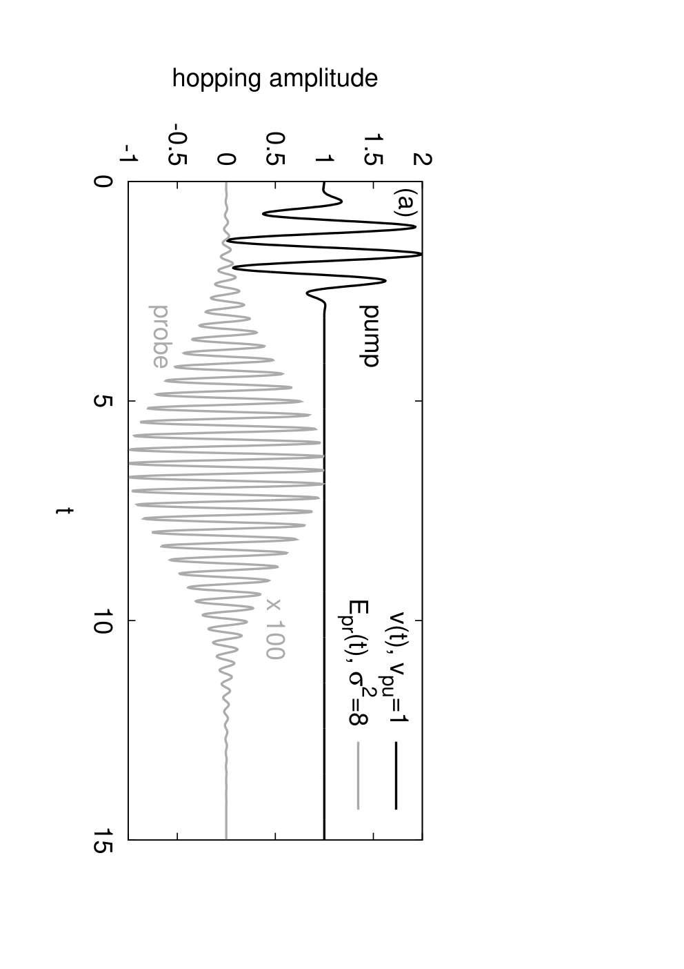
To “photo-excite” the system, we employ a time-dependent modulation of the hopping parameter ,
| (14) |
Here, is the frequency of the pump pulse, its maximum amplitude and the envelope function centered at time . In the following, we will set as the unit of energy ( as the unit of time), which corresponds to a noninteracting lattice DOS of bandwidth . The initial inverse temperature is .
To compute the XAS signal, we follow Sec. II.5 and solve the 3-orbital impurity model given by the valence-band Anderson impurity model supplemented by the core level [c.f. Eq. (13) for the local part]. The probe pulse is described by a dipolar coupling between the core level and the -orbital with index : , with . (Due to the degeneracy between the valence orbitals in our model, the dipolar coupling to the orbital would give the same results.) The probe field has the form
| (15) |
with the probe pulse frequency , and an envelope function centered at time . Unless otherwise stated, we use probe pulses with . The amplitude , which incorporates the dipole matrix element, is chosen weak enough that the absorbed energy is quadratic in [c.f. Eq. (12)]. The results below are based on an explicit treatment of this model with a relatively shallow core level, which is however still well separated in energy from the valence states.
The explicit form of the core bath (a box shaped density of states of width ) is given in Appendix B. As long as , the core-hole decay induced by this bath will lead to an additional broadening of the XAS signal, on top of the broadening resulting from the short probe pulse. The corresponding lineshape of an isolated transition is analyzed in Fig. 12 of Appendix B. The power spectrum of the probe pulse is a Gaussian. The lineshape for the single XAS absorption line then results from a convolution of the core-hole decay and this finite energy resolution of the probe. To a good approximation, the resulting lineshape is again Gaussian
| (16) |
with for the probe pulses with and for the shorter probe pulses with (see Appendix B). For simplicity we will use this Gaussian lineshape in the analysis below, unless otherwise indicated.
III.2 Half-filled model


III.2.1 Spectral functions
We first discuss the half-filled two-orbital Hubbard model and choose the interaction parameters of the manifold as , . The equilibrium spectral functions are shown for in Fig. 1(a). Because of the large Hund coupling, the half-filled high-spin states dominate the equilibrium configuration. The upper and lower Hubbard band is centered around the electron addition energy and electron removal energy , respectively, so that . In the following, we will fix such that the -electron addition and removal energies for the state are symmetric (), which implies . The core band is centered around the core removal energy ; we will fix such that , which implies . In a realistic system, the energy splitting to the core level is much larger, but for the calculation of the XAS spectrum with the present formalism, we merely need a completely occupied core level that is sufficiently separated from the levels. All the XAS results will be plotted as a function of .
The width of the upper (lower) Hubbard bands basically gives the range of kinetic energy for the triplons (singlons ), which are delocalized states if the core is filled (). In addition to the main Hubbard bands at we recognize shoulder and satellite structures at higher energies ( and ), which are more clearly seen on the log-scale plot in Fig. 1(b) (gray line). These structures originate from local spin excitations on neighboring sites (triplon insertion plus hopping to a neighboring site, which leaves behind a low-spin doublon Lysne et al. 2020), and would not be present in the atomic limit.
III.2.2 XAS in equilibrium
We now turn to the XAS signal, shown in Fig. 1(b). As in the case of the spectral function, the local multiplet energies are a good starting point for analyzing the main XAS features. Starting from the dominant state, one can create a local configuration by transferring an electron from the core to the shell. In the atomic limit, there would be a peak in the XAS signal at , broadened by the core lineshape and the probe envelope. Due to virtual charge fluctuations, the true initial state before the X-ray absorption has admixtures from , with a triplon on a different site. This makes final states accessible with a configuration , where , and the addition “” indicates that in addition to the local state a delocalized triplon has been created from a state. In the following, we will call the final state the exciton, while the final states which involve a delocalized excitation will be referred to as the continuum. The lowest continuum band, , is at , where is the energy of the delocalized triplon, which lies in the upper Hubbard band region. The exciton is therefore simply shifted by a binding energy with respect to the center of the continuum at .
Figure 1(b) shows the XAS signal for three different values of , together with the bare exciton energies (vertical lines) and the energy range of the continuum (shifted upper Hubbard band; gray line). As expected, for large , when the exciton does no longer overlap with the continuum, the exciton becomes an increasingly sharp feature and the continuum is strongly suppressed, while for small the two signals merge into a broad feature. In the strongly localized regime of large , the shape of the exciton approaches the lineshape of an isolated transition line (dashed black line), which is determined by the broadening due to the core-hole decay and the limited energy resolution of the short probe. (Here we do not use the Gaussian fit Eq. (16) to the line, but the exact atomic lineshape as computed in Appendix B.)

The slight shifts of the exciton peaks with respect to the bare excitation line can be interpreted as hybridization shifts of the energies, which would be corrected if the local states would be computed in a cluster with surrounding orbitals rather than for an isolated site. (The DMFT impurity model of course includes this environment.) Moreover, we remark that virtual admixtures to the initial state also allow different final states: There should be a continuum , corresponding to a local state with one additional electron and a delocalized hole . This signal lies outside the spectral region shown here and is strongly suppressed. Moreover, the exciton could be accompanied by satellites corresponding to additional doublon multiplets (Hund’s excitations) on other sites. However, the creation of such satellites involves high-order hopping processes and they are hence also strongly suppressed.

III.2.3 XAS after photodoping
We next discuss the XAS signal of the pump-excited system (resonant excitation with , probe pulse centered at ; see Fig. 3(a) for the pump and probe pulses). As shown in Fig. 2, the main peak of the equilibrium system is weakened, while additional spectral weight appears mainly at lower energies, but to some extent also at higher energies. To interpret this rather rich nonequilibrium spectrum, we can again start from a local picture.
| , | , | ||||||||||||
|---|---|---|---|---|---|---|---|---|---|---|---|---|---|
| , | -7 | , | -1 | , | 1 | , | -1 | ||||||
| , | -6 | , | 1 | , | 1 | ||||||||
| , | -4 | , | -1 | , | -1 | , | -1 | ||||||
| , | 0 | , | 1 | , | -1 | ||||||||
| , | 3 | , | 1 | , | 1 | , | -1 | , | 1 | , | -1 | ||
| , | 1 | , | 1 | , | 1 | , | -1 | , | 1 | , | -1 | ||
| , | -3 | , | 1 | , | 1 | , | -1 | , | 1 | , | -1 | ||
| , | 4 | , | 1 |
The nonequilibrium excitation is generating multiple possible initial configurations in addition to the state: Figure 3(b) shows the evolution of the local state occupations for a strong pump . Plotted is the quantity
| (17) |
which corresponds to the total occupation of a multiplet , and is measured from the reduced density matrix of the DMFT impurity site. (By construction, .) The red line shows the occupation, which dominates in the initial equilibrium state. A substantial fraction of these high-spin doublons is converted into other states by the pulse. In particular, the pulse creates a significant density of triplons (and the same density of singlons ), see pink line. A part of the initial kinetic energy of these delocalized excitations is then further converted into different multiplet excitations.Strand et al. 2017 Consequently, one can see an increase of the two types of low-spin doublon states, and (green and dark blue lines). Their relative density depends on the pulse amplitude. A significant population of and configurations (identical value, light-blue line) is only produced by a strong pulse.
We can now ask to what extent this local state dynamics is reflected in the XAS spectrum. In a similar way as discussed for the initial states in equilibrium, all other initial configuration can be transformed by the X-ray pulse either into exciton configurations , or into various excitation continua and satellites which involve multiplet excitations on other sites. Let us first discuss the signature of the excitons. Table 2 gives an overview over the possible initial states (first column) and the accessible exciton states (second column) and their energies . In a first approach to interpret the trXAS results in Fig. 2, one may compute the spectrum for an isolated site, but allowing for all possible initial configurations, as given by the time-dependent probabilities (17). This amounts to the ansatz
| (18) |
where and are all possible atomic initial and final states, denotes the initial state occupations, the atomic lineshape approximated by Eq. (16), and the matrix element. Since the energies and depend only on the multiplet, the sum over all states can be rewritten in terms of a sum over initial and final multiplets,
| (19) |
with the accumulated matrix element
| (20) |
for all possible transitions between the multiplet and the exciton. This matrix element takes into account that in the present simulation the X-ray pulse couples only to orbital and is not spin sensitive. The normalization by the number of states in the initial multiplet is introduced because measures the total occupation of the multiplet, not the occupation of the individual states [c.f. Eq. (17)]. The matrix elements are listed in the third column of Table 2.

In Fig. 4 we compare the nonequilibrium XAS spectrum for the stronger photoexcitation , measured at with the longer probe pulse with (violet curve), to the spectrum reconstructed from Eq. (19), where the total spectrum (black line) has been rescaled with an overall factor. The reconstruction of the trXAS signal from the nonequilibrium density matrix works relatively well, which indicates that XAS can be used to determine the dynamics of the local occupations.
Of course there are deviations from the atomic picture. On the one hand, the bare exciton lines experience small shifts with respect to the full DMFT result, which can be understood as hybridization shifts, just like in the equilibrium spectra. More importantly, for the interpretation one should take into account that in the nonequilibrium situation there are additional effects on the lineshape and position of the exciton peaks:
(i) Initial state effects: The initial states and are delocalized singlons and triplons, and their energy should therefore be taken from a broader distribution which is determined by the electron addition and removal spectrum, respectively, i.e., the unoccupied density of states within the lower Hubbard band (singlons) and the occupied density of states in the upper Hubbard band (triplons). Previous nonequilibrium DMFT simulations have shown that the initial energy distribution of excited singlons and triplons after an impulsive excitation covers almost the entire upper and lower Hubbard band,Eckstein and Werner 2011 but as these excitations lose kinetic energy by creating additional Hund’s excitations and , the singlon and triplon distribution relaxes towards the upper edge of the lower Hubbard band and lower edge of the upper Hubbard band, respectively.Strand et al. 2017 Hence one might expect a corresponding time-dependent shift and narrowing of the signals associated with the transitions and . However, in the present case this initial relaxation dynamics happens within a few hopping times (see the initial increase of and states in Fig. 3), and therefore cannot be resolved given the restrictions imposed by the energy-time uncertainty of the probe pulse. The remaining effect of the initial state delocalization is therefore an additional broadening, which is consistent with the data.
(ii) Final state effects and additional hybridization with the continuum: In the nonequilibrium state, there are additional continuum excitations compared to the initial equilibrium state. More specifically, for each exciton , we can look for states , where the local state is transformed into with a different occupation, while a state in the environment is switched from to . In equilibrium, only needs to be considered, but in the excited state there are many more possibilities. For example, the exciton can hybridize with a doublon exciton () by a transition which involves the decay of a photo-excited singlon, . Whether the initial exciton is well-defined will depend on whether or not its excitation energy overlaps with the continuum. Table 2 gives an overview over the possible processes for the present case. The first column is the initial state configuration, the second columns show accessible exciton excitations , with the given excitation energy . The subsequent columns show continuum excitations which are accessible from the exciton by a single particle exchange with the continuum; only those continuum states are shown which are in close resonance with the exciton, i.e., with energy such that , sufficiently smaller than the width of the Hubbard bands. One can see that the and excitons are already close to a continuum state if the environment is in equilibrium (their decay involves a state). For the other excitons, decay channels are activated by nonequilibrium and populations, which is in agreement with the observation that all exciton lines are broadened with respect to the atomic line-width.
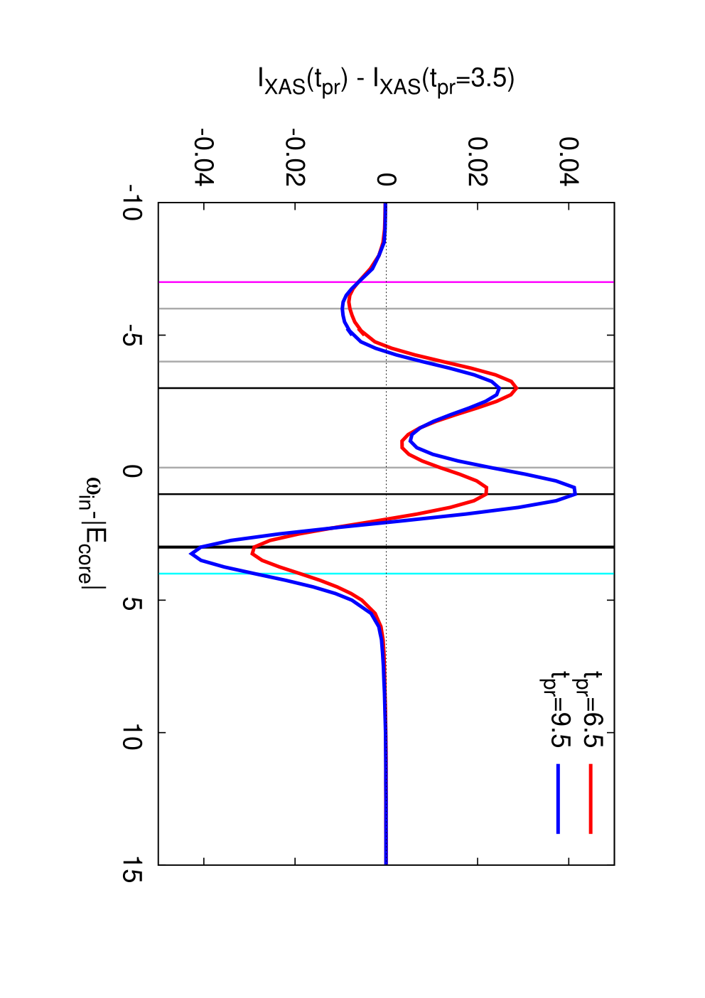
It follows from the previous discussion that the time evolution of the XAS signal allows to track the change in the population of the different local states. Because the initial dynamics during the pump is so fast that the individual multiplet peaks are difficult to resolve given the energy-time uncertainly of a sufficiently short pulse,Strand et al. 2017; Gillmeister et al. 2020 we focus on the dynamics after the pump. Figure 5 plots the difference in the signal at and (red curve) as well as and (blue curve), measured with the short probe pulse (). These curves in particular show the increasing population of the exciton (black vertical line at ), which is consistent with the increase of the occupation for times (green line in Fig. 3). They also reveal an initially strong increase followed by a slow decrease of the exciton (black vertical line at ), which tracks the behavior of the occupation (dark blue line in Fig. 3). Similarly, one can see clear signatures of the decrease in the high-spin doublon and triplon states states (red and pink lines in Fig. 3; thick black and light blue vertical lines in Fig. 5) and in the singlon states (same as pink line in Fig. 3; gray vertical lines, especially at in Fig. 5).
III.3 Quarter-filled system
III.3.1 Spectral functions
In this section, we consider the quarter-filled two-band model with , , whose equilibrium DOS is very different from the half-filled case, as one can see by comparing Fig. 1(a) and Fig. 6(a). Here, we place the core level at , and the highest energy subband of the upper Hubbard band (associated with the creation of ) at energy . This gives two conditions for the electron addition energy, , and for the core electron removal energy, , which determine the values of and : , . With these parameters, the lower Hubbard band, which represents singly occupied states, is centered at , and the subbands of the upper Hubbard band are found near (), , and , as shown in Fig. 6(a). From high to low energies, these subbands are associated with the creation of the states , and . As in the half-filled case, the spectral function of the core level is broadened by the coupling to a bath with a box-shaped density of states and bandwidth (dashed black line in Fig. 6(a)). The coupling strength to this bath is .
III.3.2 XAS in equilibrium
The equilibrium XAS signals for different values of are plotted in Fig. 6(b). In the atomic limit, the spectrum features three peaks associated with the transitions (). The corresponding energies are . With increasing core hole interaction, the XAS peaks are shifted to lower energy by . In the lattice system, for large enough , we expect exciton features near these energies, with a lineshape similar to that of the atomic system (see dashed black line for the exciton peak for ). In addition, there can be continuum features associated with the hopping of the doublon from the site with core hole into the rest of the lattice, . Since the energy difference between the initial and final state in this decay is , it is clear that for , the continuum features which do not involve any change in the doublon configuration () appear at the same energies as the exciton. We thus obtain three strongly broadened peaks which overlap with the appropriately shifted upper Hubbard band of the spectral function (gray line in Fig. 6(b)).
For , the lowest-energy exciton peak exhibits little overlap with the continuum and becomes sharp, while the middle and high-energy peaks are broadened because they overlap with continuum features associated with . For , only the highest-energy peak is affected by such a broadening. The other continuum features are evident as humps near the energies of the shifted upper Hubbard band, as indicated by the blue labels.


III.3.3 XAS after photo-doping
The XAS signals after photo-excitation with are shown in Fig. 7 for and compared to the equilibrium result (red line). Here, the pump pulse envelope is the same as in Fig. 3(a) and the probe pulse with is centered at . The black vertical lines at , , , which correspond to the final state excitons , , , respectively, show that excitations associated with the creation of doublon states () indeed explain the main equilibrium XAS features (red line). As in the half filled case, additional local states should contribute to the XAS signal after the photo-excitation. Transitions associated with empty states () should produce a peak near (pink line). Transitions associated with the three different doublon states () should result in three additional features at higher energies: for the , , doublons, we expect them to appear near , , , respectively (gray lines). Core excitations to triplons () should produce a single peak near (light blue line).

The XAS signals after photo-excitation with and , are shown in Fig. 7 by the pink-violet lines. We observe some broadenings and shifts of the main XAS peaks relative to the equilibrium spectrum, as well as the enhancement of some of the satellite features. In the energy interval , the enhancement of the signal near the exciton transitions starting from the exited states (empty initial states shown by the pink vertical line and doubly occupied states shown by grey vertical lines) is partly compensated or even overcompensated by the reduction of the peak amplitudes near the exciton transitions starting from the dominant equilibrium state (black lines). This results in a reduced signal and small energy shifts of the peaks. The enhancement of the signal associated with doublons and triplons is however clearly seen at higher energies.
Overall, the relative changes in the XAS signal are smaller than in the half-filled case (Fig. 2), which can be explained by the weaker absorption of the quarter-filled system. The evolution of the local states after the pulse with is plotted in Fig. 8 and indeed shows smaller relative changes of the different local state populations than observed in the half-filled system (Fig. 3(b)). Apart from the expected decrease in the initially dominating configurations, this figure demonstrates a strong increase in the population, which roughly matches the total increase in the populations. This is expected, since the pump pulse primarily converts two singlons on neighboring sites into a doublon and an empty site. Among the populations, we find the strongest increase for during the pump pulse, because mainly excites electrons into the highest-energy subband of the upper Hubbard band. In the dynamics after the pump, we observe the conversion of high-energy doublons into lower-energy doublons and . We also note that the conversion of a state and a neighboring state into an empty site and a triplon costs an energy , which matches the energy released by the decay of into two singlons. Hence, if the pulse creates a substantial density of and states, these can trigger the production of triplons. After the current pump pulse, these densities are however so low that the triplon population increases only slowly.

As in the half-filled case, it is an interesting question how well the trXAS spectrum can be reproduced with broadened atomic peaks, whose weights are chosen according to the nonequilibrium distribution plotted in Fig. 8. The result for and is shown in Fig. 9, which compares the nonequilibrium DMFT result (blue line) to the reconstructed spectrum (black line). In addition, we also show here the initial equilibrium spectrum (red line) and the reconstructed spectrum of the initial equilibrium state (gray line). The matrix elements listed in Table 2 have been used to convert the valence occupations into the weights of the different atomic peaks, and we again employ Gaussians with (Appendix B) to reconstruct the nonequilibrium XAS signal. The comparison with the full DMFT result shows that the actual broadening is significantly larger than in the half-filled case analyzed in Fig. 4. This is because the high-energy subband overlaps with the continuum (Fig. 6(b)), and also several of the photo-induced features are energetically close to continuum states (Table 2). (Note that while for the quarter filled system the positions of the excitonic transitions are different from the half-filled system, because the values for and differ, the energy difference between the continuum and the excitons is independent of and and therefore the same as listed in Table 2.) Many of the near-resonant exciton decay paths for involve singly occupied initial states on the lattice (continuum states with “” in the table) and are therefore active already after weak excitations, while for the half-filled system the singlons first need to be populated by the pulse. Because the resulting broadening effect is missing in the reconstructed spectrum, a better agreement with the nonequilibrium DMFT result would be obtained for . Nevertheless, at the qualitative level, we can see that the change in the reconstructed spectra (gray and black lines) correctly reproduces the photo-induced change in the DMFT results. In particular, it captures the significant broadening and shift of the lowest-energy peak, which comes from the enhanced population of empty states, and the significant relative increase of the shoulder structure around -. It also correctly describes the reduction of the main peaks near the black vertical lines, and the slight shift of the dominant peak near - to higher energy.

As in the case of the half-filled system, the evolution in the population of the local states is reflected in the trXAS signal. To illustrate this, we plot in Fig. 10 the differences (red) and (blue). For these calculations, we use the shorter probe pulse with . One notices the increase in the signal associated with the triplons (pink line) and doublons (gray line at ), which matches the evolution of the corresponding probabilities after the pump (Fig. 8). We further see a decrease in the signals near the black vertical lines (except near , where this decrease is overcompensated by the increase in the triplon signal) and the lowest-energy gray line, which is consistent with the decrease of the and populations after the pump. The kink-like structure near reflects the decrease in the population and simultaneous increase in the population.
III.3.4 Effect of the pump frequency
Since the upper Hubbard band of the quarter-filled system splits into three subbands, one might expect that the trXAS signal exhibits a characteristic dependence on the frequency of the pump pulse, which could be exploited to identify the origin of the different spectral features. In Fig. 11, we plot measurements for the three different resonant excitations to these subbands at , , : , , . Panel (a) shows the difference between the photo-doped XAS signal (measured at with the long probe pulse with ) and the equilibrium spectrum. The expected enhancement of the , and populations by the three different pulses is clearly reflected in the data, which show an increase near the corresponding gray lines with , , , respectively. (For the gray lines next to black ones, the increase is partially masked by the decrease in the population, which results in a kink-like structure.) The evolution of the XAS signal also demonstrates an increase in the empty site population after all these pulses (peaks near the vertical pink line), which is expected since all three pulses convert singlons into doublons and empty sites.
In panel (b), we plot the difference between the nonequilibrium spectra for , and the one for . This figure shows more clearly that the pulse creates more high-spin doublons relative to the pulse (maximum in the light-blue line near ), and less doublons (minimum near ). On the other hand, the pulse creates more doublons (maximum in the dark-blue line near ) and also less doublons (minimum near ). The data around the black line with furthermore show that the pulse removes states more efficiently than the other two pulses. This is because of the slightly larger total absorption for , which excites core electrons to the center of the absorption band.


IV Conclusions
We proposed a formalism to compute the dynamics of time-resolved XAS based on nonequilibrium DMFT and applied the procedure to photo-doped Mott insulators. The calculation is performed in two stages. First, we simulate the dynamics in the valence bands after a photo-excitation using DMFT. Second, the XAS signal is extracted by the explicit treatment of core orbitals in an extended impurity problem and time-dependent simulations of core-valence excitations. The equilibrium XAS signal is dominated by excitonic resonances between a core hole and valence electrons in the upper Hubbard band due to their strong interaction, while the weaker continuum features are associated with delocalized states. After a photo-excitation, the non-thermal population of local many-body states activates new excitonic features in XAS and modifies the lifetime of resonances due to additional decay channels. We calculated these effects by considering the two-band Hubbard model at half- and quarter-filling and connected the photo-induced XAS features to the activated transitions to different multiplets. The analysis exemplifies how a simple pump-probe protocol combined with XAS allows us to determine the time-dependent population of different local states in correlated solids and complements previous analyses based on time-resolved photo-emission Strand et al. 2017; Gillmeister et al. 2020; Ligges et al. 2018 or strong-field effects.Dasari et al. 2020
In previous studies, the equilibrium XAS signal has been successfully analyzed with small cluster calculations.van der Laan et al. 1986; Haverkort et al. 2012 An important outcome of our time-dependent calculation is the demonstration that such cluster calculations can be generalized to time-resolved XAS by properly adjusting the nonthermal multiplet population. Such an analysis will be particularly useful for describing realistic correlated solids, because the high computational complexity of explicit time-dependent calculations imposes severe constraints.Wang et al. 2020
Despite the similarities between the two approaches, the time-dependent DMFT formalism offers some significant benefits. In particular, small cluster calculations cannot capture the broadening associated with the decay into continuum excitations, and one may expect severe finite-size effects, because photo-induced charge carriers are mobile. Since the DMFT bath represents the infinite environment of the probed site, our nonequilibrium DMFT method does not suffer from these limitations. Moreover, by following the dynamics of the photo-induced state population we can learn how highly excited charge carriers are coupled to bosonic degrees of freedom, including orbital, antiferromagnetic, or lattice excitations. A significant technical challenge is extending the analysis to longer probe times (higher energy resolution), which will shed light on these couplings via photo-induced peak shifts and lifetime changes in trXAS.
Extending the modeling beyond on-site Hubbard interactions will allow us to follow the dynamics of crystal-field excitations in charge-transfer insulators or explore the vibrational control of - excitations by infra-red pump pulses.Marciniak et al. 2021 Finally, the presence of excitons in XAS leads to a high sensitivity to photo-induced changes in the screening, whose dynamics is essential to understand the photo-manipulation of bandgaps in correlated solids.Golež et al. 2019; Baykusheva et al. 2022
Acknowledgements.
P.W. acknowledges support from ERC Consolidator Grant 724103 and SNSF Grant No. 200021-196966, and M.E. from ERC Starting Grant No. 716648. DG is supported by Slovenian Research Agency (ARRS) under Program J1-2455 and P1-0044. The calculations were run on the Beo05 cluster at the University of Fribourg.Appendix A Rotating wave approximation
Usually, there is a large energy scale separation between the bandwidth of the valence band, which is at most of the order of a few eV, and the energies , and , which can be of the order of keV. In this case, the numerical evaluation can be simplified using a rotating wave approximation. For completeness, we summarize the corresponding equations in this appendix.
We assume that , , with . To make use of a rotating wave approximation, the Hamiltonian [Eq. (1)] is then rewritten using a canonical transformation which shifts the energy of the core band. In general, after a time-dependent basis transformation the new wavefunction satisfies the Schrödinger equation with . The choice leads to
| (21) |
where the valence Hamiltonian and the core-valence interaction remain unchanged, but the core energy in is shifted to . The dipolar Hamiltonian becomes
| (22) |
where the rapidly oscillating counter-rotating terms proportional to have been omitted. In the following, we will assume that , unless otherwise stated.
To evaluate the rate (11) within the rotating wave approximation, we first note that one can neglect the time derivative with respect to ; only the latter will give a nonzero contribution to Eq. (12) in the limit of a deep core hole. Moreover, when switching to the co-moving frame, with , one can again omit fast rotating terms, which would vanish in the integral Eq. (12). Hence, in the rotating wave approximation the absorption rate is given by
| (23) | ||||
| (24) |
and
| (25) |
In these expressions, the expectation value is understood in the rotating frame, and the subscript emphasizes that it is computed for the driven system.
Starting from Eq. (25) [and similarly from Eq. (12)] we can also reformulate the XAS intensity in term of response functions: One can express in linear response using a Kubo formula,
| (26) |
where
| (27) |
Because the core hole is initially filled, and the undriven evolution does not mix core and valence states, only the ordering contributes to , i.e., we have
| (28) |
Inserting Eq. (26) into Eq. (25) gives
| (29) |
With the hermitian symmetry , this can be rewritten as
| (30) |
If both impurity and core dynamics are diagonal in spin and orbital , the XAS intensity is the sum over the different orbital and spin contributions,
| (31) | ||||
| (32) |
where
| (33) |
Equations (25) and (30) provide two formally equivalent ways to compute . For a system out of equilibrium, it usually does not increase the computational complexity to add the driving to the simulation. In this case, it can be advantageous to calculate the explicit time evolution (25) whenever the evaluation of the two-point correlation function is more involved than the evaluation of the single-time expectation value . (As discussed in Ref. Eckstein and Werner 2021, computing higher-order correlation functions within the hybridization expansion requires vertex corrections.) However, once has been computed at all times, can be evaluated from Eq. (30) for all possible probe pulses and probe frequencies at once, while the use of Eq. (25) requires a separate simulation for each probe pulse and frequency. In the present work, we use the explicit evaluation given by Eq. (12) in the main text.
For completeness, we also relate the real-time response formula to the conventional spectral representation of the XAS signal (see also Refs. Eckstein and Werner 2021; Zawadzki et al. 2020; Chen et al. 2019 for similar discussions in the context of RIXS). In equilibrium, the response function is translationally invariant and can be represented in terms of its Fourier transform,
| (34) |
The absorption (30) becomes
| (35) |
This is just a convolution of with the square of the Fourier transform of the probe,
| (36) |
which implies the Fourier limitation of the spectral resolution due to a finite probe duration. A finite core hole lifetime corresponds to an additional broadening (see Appendix B). The spectral intensity can be represented in terms of the eigenstates
| (37) |
where are initial states (without a core hole) with statistical weight , and are final states with a core hole.


Appendix B Atomic limit
The purpose of this appendix is (i) to specify the explicit expression for the core bath and to confirm that this provides a suitable way to implement the finite core hole lifetime, and (ii), to analyze the lineshape for the atomic transitions in the present setting (finite duration of the pump and the coupling to the explicit core bath). These lineshapes are then used in the main text to analyze the spectra [c.f. Eq. (16) and the related discussion].
In the simulations we consider the half-filled system and choose , as in the main text. We use the impurity model with local Hamiltonian (13) to compute the XAS signal from Eq. (12). In the action (6), the valence hybridization term is set to zero (atomic limit), while the core bath [Eq. (9)] is taken to be the same as in the simulations in the main text: The hybridization in Eq. (9) is given in terms of its density of states
| (38) |
with , a smooth cutoff (), and a bath coupling strength . The retarded component of is then , and the other components are determined accordingly. Because the core bath is well below the chemical potential, it is completely filled () and will thus simply lead to a filling-in of a core hole state.
Without core-hole decay, the atomic XAS spectrum of the half-filled system, measured with the Gaussian probe pulse (15) features a single line, , where is the power spectrum of the probe pulse i.e., the square of the Fourier transform of ,
| (39) |
Figure 12(a) shows the explicit simulation using , for the atomic limit with the core bath (bold red line), and the power spectrum of the probe pulse (blue dashed line). The latter is rescaled and shifted such that the peak positions match. Apparently, the coupling to the core bath leads to an additional broadening. In the wide band limit, a flat bath density of states implies an approximately exponential core hole decay, corresponding to a Lorentzian broadening in the Fourier transform. Correspondingly, we compare the spectrum of the simulation with the core bath to the lineshape
| (40) |
which is obtained by convoluting a Lorentzian with width with the power spectrum (thin gray line). We find a good agreement for , which indicates that the core bath used in this study approximately reproduces the conventional exponential decay. For the reconstruction of the nonequilibrium spectra in the paper, we use for simplicity a Gaussian fit to the line [c.f. Eq. (16) in the main text], as illustrated by the black dashed line. This approximation catches the lineshape in the peak region, but not the (small) tails. For , the fit gives the width . Figure 12(b) repeats the same analysis for the shorter pulse with , leading to a best fit with .
References
- van der Laan et al. (1986) G. van der Laan, J. Zaanen, G. A. Sawatzky, R. Karnatak, and J.-M. Esteva, Phys. Rev. B 33, 4253 (1986), URL https://link.aps.org/doi/10.1103/PhysRevB.33.4253.
- Himpsel et al. (1991) F. J. Himpsel, U. O. Karlsson, A. B. McLean, L. J. Terminello, F. M. F. de Groot, M. Abbate, J. C. Fuggle, J. A. Yarmoff, B. T. Thole, and G. A. Sawatzky, Phys. Rev. B 43, 6899 (1991), URL https://link.aps.org/doi/10.1103/PhysRevB.43.6899.
- Haverkort et al. (2004) M. W. Haverkort, S. I. Csiszar, Z. Hu, S. Altieri, A. Tanaka, H. H. Hsieh, H.-J. Lin, C. T. Chen, T. Hibma, and L. H. Tjeng, Phys. Rev. B 69, 020408 (2004), URL https://link.aps.org/doi/10.1103/PhysRevB.69.020408.
- Basov et al. (2017) D. N. Basov, R. D. Averitt, and D. Hsieh, Nature Materials 16, 1077 (2017), ISSN 1476-4660, URL https://doi.org/10.1038/nmat5017.
- Giannetti et al. (2016) C. Giannetti, M. Capone, D. Fausti, M. Fabrizio, F. Parmigiani, and D. Mihailovic, Advances in Physics 65, 58 (2016), URL https://doi.org/10.1080/00018732.2016.1194044.
- de la Torre et al. (2021) A. de la Torre, D. M. Kennes, M. Claassen, S. Gerber, J. W. McIver, and M. A. Sentef, Rev. Mod. Phys. 93, 041002 (2021), URL https://link.aps.org/doi/10.1103/RevModPhys.93.041002.
- Baykusheva et al. (2022) D. R. Baykusheva, H. Jang, A. A. Husain, S. Lee, S. F. R. TenHuisen, P. Zhou, S. Park, H. Kim, J.-K. Kim, H.-D. Kim, et al., Phys. Rev. X 12, 011013 (2022), URL https://link.aps.org/doi/10.1103/PhysRevX.12.011013.
- Mitrano and Wang (2020) M. Mitrano and Y. Wang, Communications Physics 3, 184 (2020), URL https://doi.org/10.1038/s42005-020-00447-6.
- Haverkort et al. (2012) M. W. Haverkort, M. Zwierzycki, and O. K. Andersen, Phys. Rev. B 85, 165113 (2012), URL https://link.aps.org/doi/10.1103/PhysRevB.85.165113.
- Wegkamp et al. (2014) D. Wegkamp, M. Herzog, L. Xian, M. Gatti, P. Cudazzo, C. L. McGahan, R. E. Marvel, R. F. Haglund, A. Rubio, M. Wolf, et al., Phys. Rev. Lett. 113, 216401 (2014), URL https://link.aps.org/doi/10.1103/PhysRevLett.113.216401.
- Golež et al. (2019) D. Golež, L. Boehnke, M. Eckstein, and P. Werner, Phys. Rev. B 100, 041111 (2019), URL https://link.aps.org/doi/10.1103/PhysRevB.100.041111.
- Tancogne-Dejean et al. (2018) N. Tancogne-Dejean, M. A. Sentef, and A. Rubio, Phys. Rev. Lett. 121, 097402 (2018), URL https://link.aps.org/doi/10.1103/PhysRevLett.121.097402.
- Strand et al. (2017) H. U. R. Strand, D. Golež, M. Eckstein, and P. Werner, Phys. Rev. B 96, 165104 (2017), URL https://link.aps.org/doi/10.1103/PhysRevB.96.165104.
- Rincón et al. (2018) J. Rincón, E. Dagotto, and A. E. Feiguin, Phys. Rev. B 97, 235104 (2018), URL https://link.aps.org/doi/10.1103/PhysRevB.97.235104.
- Petocchi et al. (2019) F. Petocchi, S. Beck, C. Ederer, and P. Werner, Phys. Rev. B 100, 075147 (2019), URL https://link.aps.org/doi/10.1103/PhysRevB.100.075147.
- Gillmeister et al. (2020) K. Gillmeister, D. Golež, C.-T. Chiang, N. Bittner, Y. Pavlyukh, J. Berakdar, P. Werner, and W. Widdra, Nature Communications 11, 4095 (2020), URL https://doi.org/10.1038/s41467-020-17925-8.
- Georges et al. (1996) A. Georges, G. Kotliar, W. Krauth, and M. J. Rozenberg, Rev. Mod. Phys. 68, 13 (1996), URL https://link.aps.org/doi/10.1103/RevModPhys.68.13.
- Cornaglia and Georges (2007) P. S. Cornaglia and A. Georges, Phys. Rev. B 75, 115112 (2007), URL https://link.aps.org/doi/10.1103/PhysRevB.75.115112.
- Haverkort et al. (2014) M. W. Haverkort, G. Sangiovanni, P. Hansmann, A. Toschi, Y. Lu, and S. Macke, EPL (Europhysics Letters) 108, 57004 (2014), URL https://doi.org/10.1209/0295-5075/108/57004.
- Lüder et al. (2017) J. Lüder, J. Schött, B. Brena, M. W. Haverkort, P. Thunström, O. Eriksson, B. Sanyal, I. Di Marco, and Y. O. Kvashnin, Phys. Rev. B 96, 245131 (2017), URL https://link.aps.org/doi/10.1103/PhysRevB.96.245131.
- Hariki et al. (2018) A. Hariki, M. Winder, and J. Kuneš, Phys. Rev. Lett. 121, 126403 (2018), URL https://link.aps.org/doi/10.1103/PhysRevLett.121.126403.
- Hariki et al. (2020) A. Hariki, M. Winder, T. Uozumi, and J. Kuneš, Phys. Rev. B 101, 115130 (2020), URL https://link.aps.org/doi/10.1103/PhysRevB.101.115130.
- Higashi et al. (2021) K. Higashi, M. Winder, J. Kuneš, and A. Hariki, Phys. Rev. X 11, 041009 (2021), URL https://link.aps.org/doi/10.1103/PhysRevX.11.041009.
- Aoki et al. (2014) H. Aoki, N. Tsuji, M. Eckstein, M. Kollar, T. Oka, and P. Werner, Rev. Mod. Phys. 86, 779 (2014), URL https://link.aps.org/doi/10.1103/RevModPhys.86.779.
- Eckstein and Werner (2021) M. Eckstein and P. Werner, Phys. Rev. B 103, 115136 (2021), URL https://link.aps.org/doi/10.1103/PhysRevB.103.115136.
- Werner et al. (2021) P. Werner, S. Johnston, and M. Eckstein, Europhysics Letters 133, 57005 (2021), URL https://doi.org/10.1209/0295-5075/133/57005.
- Werner and Eckstein (2021) P. Werner and M. Eckstein, Phys. Rev. B 104, 085155 (2021), URL https://link.aps.org/doi/10.1103/PhysRevB.104.085155.
- Chen et al. (2019) Y. Chen, Y. Wang, C. Jia, B. Moritz, A. M. Shvaika, J. K. Freericks, and T. P. Devereaux, Phys. Rev. B 99, 104306 (2019), URL https://link.aps.org/doi/10.1103/PhysRevB.99.104306.
- Wang et al. (2020) Y. Wang, Y. Chen, C. Jia, B. Moritz, and T. P. Devereaux, Phys. Rev. B 101, 165126 (2020), URL https://link.aps.org/doi/10.1103/PhysRevB.101.165126.
- Eckstein and Werner (2010) M. Eckstein and P. Werner, Phys. Rev. B 82, 115115 (2010), URL https://link.aps.org/doi/10.1103/PhysRevB.82.115115.
- Schüler et al. (2020) M. Schüler, D. Golež, Y. Murakami, N. Bittner, A. Herrmann, H. U. Strand, P. Werner, and M. Eckstein, Computer Physics Communications p. 107484 (2020), ISSN 0010-4655, URL http://www.sciencedirect.com/science/article/pii/S0010465520302277.
- Lysne et al. (2020) M. Lysne, Y. Murakami, and P. Werner, Phys. Rev. B 101, 195139 (2020), URL https://link.aps.org/doi/10.1103/PhysRevB.101.195139.
- Eckstein and Werner (2011) M. Eckstein and P. Werner, Phys. Rev. B 84, 035122 (2011), URL https://link.aps.org/doi/10.1103/PhysRevB.84.035122.
- Ligges et al. (2018) M. Ligges, I. Avigo, D. Golež, H. U. R. Strand, Y. Beyazit, K. Hanff, F. Diekmann, L. Stojchevska, M. Kalläne, P. Zhou, et al., Phys. Rev. Lett. 120, 166401 (2018), URL https://link.aps.org/doi/10.1103/PhysRevLett.120.166401.
- Dasari et al. (2020) N. Dasari, J. Li, P. Werner, and M. Eckstein, Phys. Rev. B 101, 161107 (2020), URL https://link.aps.org/doi/10.1103/PhysRevB.101.161107.
- Marciniak et al. (2021) A. Marciniak, S. Marcantoni, F. Giusti, F. Glerean, G. Sparapassi, T. Nova, A. Cartella, S. Latini, F. Valiera, A. Rubio, et al., Nature Physics 17, 368 (2021), URL https://doi.org/10.1038/s41567-020-01098-8.
- Zawadzki et al. (2020) K. Zawadzki, A. Nocera, and A. E. Feiguin, A time-dependent scattering approach to core-level spectroscopies (2020), eprint 2002.04142.