A fast direct solver for two dimensional quasi-periodic multilayered media scattering problems, Part II

The linear system that results from the integral equation formulation in [6] results in a block linear system where each block row equation enforces a different part of the requirements of the integral formulation: boundary conditions through the interfaces, the periodicity and the radiation condition. Following the solution technique in [6], the solution to the block system can be constructed in block form requiring the inverse of a Schur complement operator that is block tri-diagonal where the off-diagonal blocks are low-rank and the diagonal blocks can be written as the sum of a full-rank matrix with low-rank matrices. Thus the inverse can be applied via a Woodbury formula. Each full rank diagonal block matrix corresponds to the discretization of an integral operator on each interface. These matrices can be inverted quickly via a fast direct solver such as the Hierarchically Block Separable (HBS) [8, 9, 4], the Hierarchically Semi-Separable (HSS) [15, 13, 14], the Hierarchical interpolative factorization (HIF) [10], and the $\mathcal{H}$ and $\mathcal{H}^{2}$-matrix methods [2, 3]. The low-rank matrices in the Schur complement are made up of a sum of low-rank matrices corresponding to the interaction of an interface with its neighbors and matrices that help enforce the periodicity and radiation conditions. The fast solver in this manuscript constructs the low-rank factors in the same manner as in [1].

The fast inverse of the discretized boundary integral equations on the diagonal blocks allows the solver to scale linearly with respect to the number of unknowns placed on each interface, and the Schur complement formulation allows the solver to scale linearly with respect to the total number of interfaces. The fast direct solver in this manuscript is ideal for optimal design problems, since the additional cost for changing an interface geometry and/or a layer wave number scales linearly with the number of discretization points on the affected interfaces instead of the total number of unknowns on the entire structure. Once the solver is built, new incident angles can also be handled with small extra cost as the most expensive calculations in building the solver is independent of incident angle or Bloch phase.

The manuscript begins by briefly reviewing the linear system that results from the discretization of the robust integral formulation for equation (1) from [6] in Section 2. Next the new fast direct solver is presented in Section 3. Section 4 describes extensions of the proposed solution technique that make it useful for practical applications. Section 5 illustrates the performance of the solver for a selection of test problems. Finally, Section 6 concludes the manuscript and discusses future directions.

The matrix $\mathsf{A}$ in equation (2) is (almost always) the largest matrix in the linear system. Fortunately $\mathsf{A}$ has structure that makes it amenable to accelerated linear algebra. We first note that $\mathsf{A}$ is a block tri-diagonal matrix

where the diagonal block $\mathsf{A}_{i,i}$ corresponds to the self interactions of the $i^{\rm th}$ interface in the unit cell and its interaction with the adjacent left and right neighbor periods and the off-diagonal block $\mathsf{A}_{i,j}$ corresponds to the interaction between the $i^{\rm th}$ interface and the interface above when $j=i-1$ or the interface below when $j=i+1$. For simplicity of presentation, we denote the diagonal blocks as follows:

where $\mathsf{A}_{i,i}^{s}$ denotes the interaction of interface $i$ inside the unit cell with itself and $\mathsf{A}_{i,i}^{pm}$ denotes the interaction between the $i^{\rm th}$ interface in the unit cell and the left and right copies of it. The superscripts “$s$” and “$pm$” stand for “self” and the left and right period (plus and minus) interactions respectively. This matches notation in [1].

With this notation, the matrix $\mathsf{A}$ can be written as

where $\mathsf{A}_{0}$ is a block diagonal matrix

All the non-self interaction matrices, including interactions between the neighboring periods of an interface and the interactions between vertically neighboring interfaces, are low-rank. For example $\mathsf{A}_{i,i}^{pm}$ and $\mathsf{A}_{1,2}$ are low-rank. This means that each of the blocks in the block tri-diagonal matrix in the right hand side of equation (7) are low-rank.

The rearrangement of the auxiliary unknowns $\bm{c}$ and $\bm{a}$ via the ordering defined in equation (3) changes the sparsity pattern of the non-principal block matrices in (4). This section presents the sparsity and entries of the reordered matrices.

The matrix $\hat{\mathsf{B}}$ is $\begin{bmatrix}\mathsf{B}&\mathsf{0}\end{bmatrix}$ with its columns reordered according to the new ordering of the unknowns and is defined as follows

where $\mathsf{B}_{i,i}$ and $\mathsf{B}_{i,i+1}$ correspond to the interaction of the $i^{\rm th}$ interface with the unknowns defined on the proxy circle for the $i^{\rm th}$ and $(i+1)^{\rm th}$ layer respectively.

The matrix $\hat{\mathsf{C}}$ is the matrix $\begin{bmatrix}\mathsf{C}\\ \mathsf{Z}\end{bmatrix}$ with its rows reordered as follows

where $\mathsf{Z}_{U}$ is the evaluation of the potential from the boundary charge density on the first interface on the top of the unit cell, $\mathsf{Z}_{D}$ is the evaluation of the potential from the boundary charge density on the last interface on the bottom of the unit cell, and $\mathsf{C}_{i,i-1}$ and $\mathsf{C}_{i,i}$ evaluate the potential due to the charge boundary density on the $(i-1)^{\rm th}$ and $i^{\rm th}$ interface on the left $L$ and right $R$ vertical walls of the unit cell in the $i^{\rm th}$ layer to enforce periodicity.

The matrix $\hat{\mathsf{Q}}$ is a block diagonal matrix obtained from reordering the rows and columns of $\begin{bmatrix}\mathsf{Q}&\mathsf{0}\\ \mathsf{V}&\mathsf{W}\end{bmatrix}$. The block entries are defined as follows

where $\mathsf{V}_{U}$ and $\mathsf{V}_{D}$ are the only non-trivial blocks in $\mathsf{V}$ corresponding to evaluating the potential at $y=y_{U}$ and $y=y_{D}$ due to the proxy circle of the top and bottom layer; $\mathsf{W}_{U}$ and $\mathsf{W}_{D}$ are the non-trivial blocks in $\mathsf{W}$ corresponding to evaluating the Rayleigh-Block expansion at $y=y_{U}$ and $y=y_{D}$; $\mathsf{Q}_{i,i}$ evaluates the potential on the vertical walls due to the proxy circle of the $i$th layer.

Thanks to the block sparsity pattern of $\mathsf{A}$, $\hat{\mathsf{B}}$, $\hat{\mathsf{C}}$ and $\hat{\mathsf{Q}}$ the Schur complement matrix $\mathsf{S}$ defined in (6) is block tri-diagonal. The non-zero blocks of $\mathsf{S}$ are defined as follows

Recall that $\mathsf{S}$ is block tri-diagonal where the blocks are defined by (9). We choose to write $\mathsf{S}$ as the sum of a full rank block diagonal matrix and a block tri-diagonal matrix whose blocks are low-rank. Specifically, we express $\mathsf{S}$ as

where $\mathsf{A}_{0}$ is defined in (8) and $\mathsf{P}$ can be defined blockwise as

Since all the blocks in $\mathsf{P}$ correspond to non-self interactions, they are low-rank. Let $\mathsf{P}\approx\mathsf{LR}$ denote the low-rank factorization of $\mathsf{P}$. Then an approximate solution to (11) can be obtained via a Woodbury formula

Since each of the diagonal blocks of $\mathsf{A}_{0}$ is the discretized integral equation on an interface, they are amenable to fast direct solvers such as the HBS, HSS, HOLDR, etc methods. Thus $\mathsf{A}_{0}^{-1}$ can be approximated for a cost that scales linearly with respect to the number of discretization points on the interfaces. The remaining complexity lies in creating the low-rank factorization of $\mathsf{P}$ and inverting the matrix $\mathsf{X}_{\rm wood}=\mathsf{I}+\mathsf{R}\mathsf{A}_{0}^{-1}\mathsf{L}$.

The low-rank factorization of $\mathsf{P}$ is handled block wise. For each non-zero block in $\mathsf{P}$, we build the factorization for each matrix in the sum independently exploiting the associated physics. For example, in creating the low-rank factorization of the block $\mathsf{P}_{i,i}$, we create the low-rank factorization of $\mathsf{A}^{pm}_{i,i}$, $\hat{\mathsf{B}}_{i,i}\hat{\mathsf{Q}}^{\dagger}_{i,i}\hat{\mathsf{C}}_{i,i}$, and $\hat{\mathsf{B}}_{i,i+1}\hat{\mathsf{Q}}^{\dagger}_{i+1,i+1}\hat{\mathsf{C}}_{i+1,i}$ independently. Let the low-rank factors be defined as follows: $\mathsf{A}_{i,i}^{pm}\approx\mathsf{L}_{i,i}^{pm}\mathsf{R}_{i,i}^{pm}$, $\hat{\mathsf{B}}_{i,i}\hat{\mathsf{Q}}^{\dagger}_{i,i}\hat{\mathsf{C}}_{i,i}\approx\mathsf{L}_{i,i,i}\mathsf{R}_{i,i,i}$, and $\hat{\mathsf{B}}_{i,i+1}\hat{\mathsf{Q}}^{\dagger}_{i+1,i+1}\hat{\mathsf{C}}_{i+1,i}\approx\mathsf{L}_{i,i+1,i}\mathsf{R}_{i,i+1,i}$. Then $\mathsf{P}_{i,i}$ can be approximated by

The technique for creating the low-rank factorization of the matrices $\mathsf{A}^{pm}_{i,i}$, $\mathsf{A}_{i,i-1}$, and $\mathsf{A}_{i,i+1}$ is presented in Section 3.1.1 of [1]. Section 3.2 presents the technique for creating the low-rank factorization of $\hat{\mathsf{B}}_{i,i}\hat{\mathsf{Q}}^{\dagger}_{i,i}\hat{\mathsf{C}}_{i,i}$. The low-rank factorization of $\hat{\mathsf{B}}_{i,i+1}\hat{\mathsf{Q}}^{\dagger}_{i+1,i+1}\hat{\mathsf{C}}_{i+1,i}$ can be created in a similar manner.

The only thing remaining is a fast inversion technique for the matrix $\mathsf{X}_{\rm wood}$. It happens to be the case that this matrix is block tri-diagonal. Thus it can be inverted rapidly via a block version of the Thomas algorithm presented in the Appendix of [1].

Creating the low-rank factorization of $\mathsf{B}_{i,i}\mathsf{Q}^{\dagger}_{i,i}\mathsf{C}_{i,i}$ requires dealing with $\mathsf{Q}_{i,i}^{\dagger}$. As mentioned in [6], filling the entries of the matrix $\mathsf{Q}_{i,i}^{\dagger}$ is not numerically stable. To avoid this, we use the truncated SVD-based pseudoinverse.

The matrices of the form $\mathsf{Q}^{\dagger}_{i,i}\mathsf{C}_{i,i}$ can be approximated by

One way of building a low-rank approximation for the matrix product $\mathsf{B}_{i,i}\mathsf{Q}^{\dagger}_{i,i}\mathsf{C}_{i,i}$ is to let

where $\mathsf{L}_{i,i,i}$ is of size $N_{i}\times l_{i}$, $\mathsf{R}_{i,i,i}$ is of size $l_{i}\times N_{i}$ and $l_{i}$ is the number of singular values of $\mathsf{Q}_{i,i}$ that are greater than $\epsilon_{Schur}$. Unfortunately, $l_{i}$ is far from the optimal rank and thus the resulting low-rank factorization of $\mathsf{P}_{i,i}$ is far larger than it needs to be. This has many implications including artificially limiting the number of layers that can be simulated on a machine.

To create a closer to optimal rank factorization of $\mathsf{B}_{i,i}\mathsf{Q}^{\dagger}_{i,i}\mathsf{C}_{i,i}$, we create a low rank factorization of $\mathsf{B}_{i,i}$ and express the low-rank factorization of $\mathsf{B}_{i,i}\mathsf{Q}^{\dagger}_{i,i}\mathsf{C}_{i,i}$ in terms of those factors. Let $\mathsf{B}_{i,i}\approx\mathsf{L}_{B,ii}\mathsf{R}_{B,ii}$ denote the low-rank factorization of $\mathsf{B}_{i,i}$. Then

In practice, the inner dimensions of this factorization are smaller than $l_{i}$ as the matrix $\mathsf{B}_{i,i}$ corresponds to interactions between distant points while the matrix $\mathsf{Q}$ is nearly full rank. While the second approach requires an additional low-rank factorization, the cost of doing this is more than made up for by the reduced rank and the fact that these factors can be used for all Bloch phase $\alpha$. Additionally, a fast algorithm is used to create the low-rank factorizations of the $\mathsf{B}_{i,i}$ and $\mathsf{B}_{i,i+1}$ matrices. Details for constructing that factorization are provided in [5].

Solving a multilayered media scattering problem for many incidents angles happens frequently in applications. For example, in creating a Bragg diagram, the solution for a large collection of incident angles in the range of $-\pi$ to $0$ is needed[11]. For each incident angle, there is a corresponding Bloch phase. Some incident angles share a Bloch phase. This means that entries in (4) change. Since in most of these matrices the dependence on Bloch phase is a scalar multiplication, the bulk of the precomputation can be reused for all Bloch phases. For example, this is the case in the matrices that make up $\mathsf{A}_{i,i}^{pm}$. This means that the low-rank factorization of this matrix can be used for all Bloch phases. It just needs to be scaled by the Bloch phase $\alpha$ correctly. An example of a matrix that is incident angle dependent and not just Bloch phase is the matrix $\mathsf{W}$. Thanks to the properties of phase shifts, it is possible to build $\mathsf{W}$ for all incident angles that share a Bloch phase. Section 3.2 of [1] details this incident angle blocking. This allows for one direct solver to be built for all incident angles that share a Bloch phase. A detailed list classifying operations by dependence on Bloch phase and incident angle is given at the beginning of section 5.

For applications where there is a desire to solve problems with a change in an interface and/or wave number, the solution technique presented in this manuscript only requires updating the matrices associated with that layer or interface. In fact, the cost of updating the solver scales linearly with the number of discretization points on the affected interfaces. This means that updating the solver is much more efficient than building a new one from scratch. Specifically, the speed-up of updating the solver over building a new solver from scratch is the total number of interfaces divided by the number of interfaces changed. If for each modified geometry the solution is desired for the same collection of incident angles, all the Bloch phase dependent precomputations that are not related to the changed interfaces or layers can be reused.

This section illustrates the scaling of the direct solver presented in this manuscript. We consider a collection of problems where the number of layers varies from 3 layers (2 interfaces) to 65 layers (64 interfaces). The interface geometries are defined by the following two curves $\gamma_{1}$ and $\gamma_{2}$ repeated alternatively:

for $t\in[0,1]$, where $\{a_{j}\}_{j=1}^{30}$ and $\{b_{j}\}_{j=1}^{30}$ are random numbers in $[0,1)$ sorted in descending order. Figure 3 illustrates the two interface geometries. In each experiment, $\gamma_{1}$ and $\gamma_{2}$ are discretized with the same number of points $N_{i}$. The value of $N_{i}$ is doubled ($1280\leq N_{i}\leq 20480$) to demonstrate the linear scaling of the solver. The wave number of each layer alternates between $10$ and $10\sqrt{2}$. For problems with $64$ interfaces, we exploit the fact that the interfaces and wave numbers are the same to decrease the memory needed by the solver. The time in seconds for each part of the precomputation using the new solver are presented in Table 1.

For a fixed structure, each part of the solution steps scales linearly with respect to $N_{i}$, the number of discretization points per interface. And for fixed $N_{i}$, each of the steps scales linearly with respect to the number of interfaces (or the number of layers). For all tests, Precomputaion I accounts for more than $90\%$ of the total computational cost. Precomputation II accounts for about $5\%$ of the total cost. Thus the Bloch phase independent parts of the direct solver dominate the computational cost of building the direct solver.

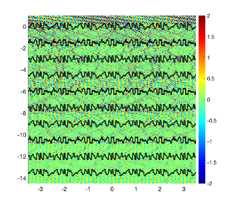
This section illustrates the performance of the direct solver when the solution is desired for many different incident angles. Specifically, we consider the 11-layer geometry illustrated in Figure 6(a) and approximate the solution using the new solver for $287$ different incident angles with $24$ different Bloch phases. Figure 5 illustrates the real part of the total field for one incident angle. The interfaces in the 11-layer structure consist of three different corner geometries, which are referred to as “corner1”, “corner2” and “corner3”, repeated in order. Each of the interfaces contains 40 to 50 right-angle corners. With the five levels of dyadic refinement into each corner there are 10,000 to 15,000 discretization points per interface. Figure 4 provides more details about the corner geometries including how many discretization points were used on each geometry. The wave number in each layer alternates between $40$ and $40\sqrt{2}$. As stated previously, the solver does group incident angles that share a Bloch phase allowing these incident angles to be solved together.

With this discretization, the average flux error for the $287$ incident angles are $4.5\times 10^{-8}$. Table 2 reports the time in seconds for each of the steps. The incident angle used to create Figure 5 is a Wood’s anomaly. Even in this example, the flux error is still on the order of $10^{-8}$, demonstrating that the proposed solution technique is robust at Wood’s anomalies.

Table 5 in the Appendix reports the performance of the solver from [1] for solving this problem. As in the previous section, the times for Precomputation I and II for the two solvers are roughly the same. The time for Precomputation III for the new solver is twice as fast per Bloch phase as the original solver for this problem. This is expected since the new solver no longer requires applying $\mathsf{A}^{-1}$ to $\hat{\mathsf{B}}$ thus reducing the cost of Precomputation III. The time for the solve step are essentially the same for both solvers.

This section illustrates the performance of the proposed direct solver for problems where there is a change in the geometry such as changing an interface or the wave number in a layer. Specifically, we consider the same 11-layer geometry as in Section 4.1 but change one interface geometry or change the wave number in a layer. For the change of interface geometry experiment, the fourth interface from the top $\Gamma_{4}$ is replaced by the “hedgehog” geometry as illustrated in Figure 6. The hedgehog geometry consists of 17 sharp corners and cannot be written as the graph of a function defined on the $x$-axis. The number of discretization points on the new interface needed to maintain the same accuracy as the original problem is $N_{4}=14,496$. For the change of wave number experiment, the wave number in the second layer from the top of the 11-layer structure $\omega_{2}$ is changed from $40\sqrt{2}$ to $30$. For these experiments, the incident angle is fixed at $\theta^{inc}=-\frac{\pi}{5}$. Recall that the solver is able to reuse a large portion of the precomputation in these experiments and only have to process matrices that involve the “new” portions of the geometry. Table 3 reports the time in seconds for each step as well as the flux error for each experiment. Each step in the precomputation is substantially less expensive. The smallest decrease is in Precomputation III which is only a factor $2-3$ faster than the same step when building a new solver from scratch. Precomputation I is slower for replacing a wave number than it is for replacing an interface because replacing the wave number involves changing matrices for two interfaces. Even so, building the solver using the method presented in this manuscript for the case of replacing a wave number is roughly $5.3$ times faster than building a new solver from scratch for the problem. There is roughly a $8.9$ times speed-up for using the solver presented in this manuscript for the replaced interface problem instead of building a solver from scratch. These speed-up numbers will be even greater for more than one Bloch phase. In comparison with the solver in [1] for these problems (Table 6 in the Appendix), the new solver is faster in Precomputation III.

References

- [1] Y. Zhang and A. Gillman. A fast direct solver for two dimensional quasi-periodic multilayered media scattering problems. BIT Numerical Mathematics, 2020.
- [2] S. Börm. Efficient numerical methods for non-local operators, volume 14 of EMS Tracts in Mathematics. European Mathematical Society (EMS), Zürich, 2010.
- [3] S. Börm and W. Hackbusch. Approximation of boundary element operators by adaptive -matrices. In Foundations of computational mathematics: Minneapolis, 2002, volume 312 of London Math. Soc. Lecture Note Ser., pages 58–75. Cambridge Univ. Press, Cambridge, 2004.
- [4] J. Bremer, A. Gillman, and P. Martinsson. A high-order accurate accelerated direct solver for acoustic scattering from surfaces. BIT Numerical Mathematics, 55:141–170, 2015.
- [5] Y. Zhang, A. Gillman, and S. Veerapaneni. A fast direct solver for integral equations on locally refined boundary discretizations and its application to multiphase flow simulations. arXiv, 2108.07205, 2022
- [6] M. Cho and A. Barnett. Robust fast direct integral equation solver for quasi-periodic scattering problems with a large number of layers. Optics Express, 23(2):1775–1799, 2015.
- [7] A. Gillman and A. Barnett. A fast direct solver for quasiperiodic scattering problems. Journal of Computational Physics 248:309–322, 2013.
- [8] A. Gillman, P. Young, and P. Martinsson. A direct solver complexity for integral equations on one-dimensional domains. Frontiers of Mathematics in China, 7:217–247, 2012.
- [9] K. Ho and L. Greengard. A fast direct solver for structured linear systems by recursive skeletonization. SIAM Journal of Scientific Computing, 34(5):2507–2532, 2012.
- [10] K. Ho and L. Ying. Hierarchical interpolative factorization for elliptic operators: Integral equations. Communications on Pure and Applied Mathematics, 69(7):1314–1353, 2015.
- [11] G. A. Kalinchenko and A. M. Lerer. Wideband all-dielectric diffraction grating on chirped mirror. Journal of Lightwave Technology, 28:2743–2749, 2010.
- [12] G. Marple, A. Barnett, A. Gillman, and S. Veerapaneni. A fast algorithm for simulating multiphase flows through periodic geometries of arbitrary shape. SIAM Journal of Scientific Computing, 38(5):B740–B772, 2016.
- [13] Z. Sheng, P. Dewilde, and S. Chandrasekaran. Algorithms to solve hierarchically semi-separable systems. In System theory, the Schur algorithm and multidimensional analysis, volume 176 of Operator Theory: Advances and Applications, pages 255–294. Birkhäuser, Basel, 2007.
- [14] J. Xia, S. Chandrasekaran, M. Gu, and X. Li. Fast algorithms for hierarchically semiseparable matrices. Numerical Linear Algebra with Applications, 17(6):953–976, 2010.
- [15] J. Xia, S. Chandrasekaran, M. Gu, and X. S. Li. Superfast multifrontal method for large structured linear systems of equations. SIAM Journal on Matrix Analysis and Applications, 31(3):1382–1411, 2009.
Appendix A Numerical Results for the algorithm presented in [1]
For fair comparison, a new implementation of the solver in [1] is rerun on the same desktop used for the numerical section of this manuscript. The results are summarized below.
The direct solver presented in [1] solves the block system (2) via the following block solve