跳到论文正文
W Papers独立论文阅读器 arXiv:2204.06597 论文正文 计算阅读时间 · 0%
引用这篇论文根据当前论文元数据生成,正式投稿前建议核对。


License: arXiv.org perpetual non-exclusive license
arXiv:2204.06597v2 [math.GT] 11 Mar 2023

Almost Simple Linear Graphs, Homology Cobordism and Connected Heegaard Floer Homology

Çağrı Karakurt Address: Department of Mathematics, Boğazıçı University, Bebek, 34342 Istanbul, Turkey. Email address: cagri.karakurt@boun.edu.tr URL: http://web0.boun.edu.tr/cagri.karakurt/ and Oğuz Şavk Address: Department of Mathematics, Boğazıçı University, Bebek, 34342 Istanbul, Turkey and Max Planck Institut für Mathematik, Vivatsgasse 7, 53111 Bonn, Germany. Email address: oguz.savk@boun.edu.tr, savk@mpim-bonn.mpg.de URL: https://sites.google.com/view/oguzsavk/
Abstract.

Continuing our previous work in [KŞ20], we effectively compute connected Heegaard Floer homologies of two families of Brieskorn spheres realized as the boundaries of almost simple linear graphs. Using Floer theoretic invariants of Dai, Hom, Stoffregen, and Truong, we show that these Brieskorn spheres also generate infinite rank summands in the homology cobordism group. Our computations also have applications to the concordance of classical knots and 00-concordance of 22-knots.

1. Introduction

Since the 1980s, the homology cobordism group Θℤ3\Theta^{3}_{\mathbb{Z}} (see Section 3.1) has been a central object in low-dimensional topology [Man18]. Although its algebraic structure is still mysterious, the recent achievement of Dai, Hom, Stoffregen, and Truong indicates that it is very complicated. Previously, it is known that Θℤ3\Theta^{3}_{\mathbb{Z}} has infinitely generated subgroups ℤ∞\mathbb{Z}^{\infty} [Fur90], [FS90] and infinite summands ℤ\mathbb{Z} [Frø02], [OS03a].

Theorem 1.1 (Theorem 1.1, [DHST18]).

Let {Xn=Σ(2n+1,4n+1,4n+3)}n=1∞\{X_{n}=\Sigma(2n+1,4n+1,4n+3)\}^{\infty}_{n=1} be a family of Brieskorn spheres. Then the homology cobordism group Θℤ3\Theta^{3}_{\mathbb{Z}} has an infinite rank summand ℤ∞\mathbb{Z}^{\infty} generated by the homology cobordism classes [Xn]n=1∞[X_{n}]^{\infty}_{n=1}.

The elegant proof of Dai, Hom, Stoffregen, and Truong relies on the construction and computation of a linearly independent set of invariants of Θℤ3\Theta^{3}_{\mathbb{Z}} originated from involutive Heegaard Floer homology, introduced by Hendricks and Manolescu [HM17]. Their proof also subsumes the several techniques in the theoretical continuation of involutive Heegaard Floer homology [DM19a], [DS19], [HMZ18] and [HHL21].

The manifolds mentioned in Theorem 1.1 are carefully selected in the sense that they have sufficiently complicated graded roots and arbitrarily large Ozsváth-Szabó dd-invariants. Even though classical and involutive Heegaard Floer homologies are known to be not homology cobordism invariants, their refinement connected Heegaard Floer homology, defined by Hendricks, Hom, and Lidman, turns out to be an invariant of Θℤ3\Theta^{3}_{\mathbb{Z}}. It essentially detects the sufficient complexity of graded roots and corresponds to the homology of monotone subroots of graded roots [HHL21].

In this article, we efficiently compute connected Heegaard Floer homologies of two families of Brieskorn spheres Σ⁡(p,q,r)\Sigma(p,q,r) realized as the boundaries of almost simple linear graphs, see Section 2.2. Here, p,qp,q and rr are chosen as pairwise coprime positive integers with p​q+p​r−q​r=1pq+pr-qr=1. Clearly, parameters of XnX_{n} satisfy the latter identity.

Theorem 1.2.

Consider the following two families of Brieskorn spheres:

{Yn=Σ(2n+1,3n+2,6n+1)}n=1∞and{Zn=Σ(2n+1,3n+1,6n+5)}n=1∞.\{Y_{n}=\Sigma(2n+1,3n+2,6n+1)\}^{\infty}_{n=1}\ \ \text{and}\ \ \{Z_{n}=\Sigma(2n+1,3n+1,6n+5)\}^{\infty}_{n=1}.

Then their monotone subroots are shown in Figure 1. Therefore, their connected Heegaard Floer homologies are given in Table 1.

Refer to caption
Figure 1. Monotone subroots of {Yn}n=1∞\{Y_{n}\}^{\infty}_{n=1} and {Zn}n=1∞\{Z_{n}\}^{\infty}_{n=1}.
H​FconnHF_{\mathrm{conn}} n≥1n\geq 1 odd n≥2n\geq 2 even
{Yn}\{Y_{n}\} 𝔽OPEN(2​n−2))​(n)\mathbb{F}_{(2n-2))}(n) 𝔽OPEN(2​n−2))​(n)⊕𝔽OPEN(n−2))​(n/2)\mathbb{F}_{(2n-2))}(n)\oplus\mathbb{F}_{(n-2))}(n/2)
{Zn}\{Z_{n}\} 𝔽OPEN(2​n−2))​(n)⊕𝔽OPEN(n+1))​((n+1)/2)\mathbb{F}_{(2n-2))}(n)\oplus\mathbb{F}_{(n+1))}((n+1)/2) 𝔽OPEN(2​n−2))​(n)\mathbb{F}_{(2n-2))}(n)
Table 1. The connected Heegaard Floer homologies of {Yn}n=1∞\{Y_{n}\}^{\infty}_{n=1} and {Zn}n=1∞\{Z_{n}\}^{\infty}_{n=1}.

Besides the family of Dai, Hom, Stoffregen, and Truong, our additional two families are the boundaries of almost simple linear graphs for odd values of pp. When pp is even, by [KŞ20], we always have d=−2​μ¯d=-2\bar{\mu} where dd is the Ozsváth-Szabó dd-invariant [OS03b] and μ¯\bar{\mu} is the Neumann-Siebenmann μ¯\bar{\mu}-invariant [Neu80] and [Sie80]. This is also the case for involutive correction terms d¯=d¯\underline{d}=\overline{d}, see [DM19a]. In this case, their connected Heegaard Floer homologies are trivial, so they do not provide valuable information for the homology cobordism group Θℤ3\Theta^{3}_{\mathbb{Z}}. Hence, the interesting families of almost simple linear graphs arise only when pp is odd.

For large values of nn, the full graded roots of the Brieskorn spheres we consider are quite complicated and intractable even with the help of computer programs. On the other hand, monotone subroots are sufficient to determine the corresponding connected Heegaard Floer homology and they have relatively simple descriptions in terms of packed sequences that we introduced in Section 4. By the work of Némethi [Ném05], Dai [Dai18], and Dai and Manolescu [DM19a], the graded roots are characterized by Laufer sequences and monotone subroots can be parametrized by using dd- and μ¯\bar{\mu}-invariants. Moreover, the μ¯\bar{\mu}-invariant can be read off from a graded root and the dd-invariant also lies on the graded root.

In this work, we relate Laufer sequences with dd-invariants in terms of the Ozsváth-Szabó algorithm, see Proposition 2.3. Therefore, we are able to compute the minimal graded subroot of the whole graded root including the monotone subroot for infinite families of plumbings, for a comparison see Remark 4.22.

Our computation procedure is indicated schematically in Figure 2. In historical order, it is a mixture of the work of Ozsváth and Szabó [OS03b], Némethi [Ném05], Can and the first author [CK14], Dai and Manolescu [DM19a], Öztürk and the first author [KO18], and Hendricks, Hom, and Lidman [HHL21], and the authors [KŞ20]. Note that the initial step in the scheme heavily depends on our previous joint work [KŞ20] in which we characterized characteristic classes supporting good full paths for almost simple linear graphs and then computed their dd-invariants.

Describe characteristic classes that support good full paths and realize the dd-invariantFind positions of these classes in the Laufer sequenceCompute semigroup elements restricted to these positions(1)(1)(2)
Evaluate delta sequences with respesct to the semigroup elementsDraw the corresponding graded root and extract the monotone subrootCalculate the connected Heegaard Floer homology(3)(3)(4)
Figure 2. User’s guide to our computation procedure.

Using the involutive Floer theoretic invariants of Dai, Hom, Stoffregen, and Truong, we present new families of homology spheres generating infinite rank summands in the homology cobordism group. With the help of gauge theoretic invariants, we also completely compare their homology cobordism classes.

Theorem 1.3.

The homology cobordism classes [Yn]n=1∞[Y_{n}]^{\infty}_{n=1} and [Zn]n=1∞[Z_{n}]^{\infty}_{n=1} also generate ℤ∞\mathbb{Z}^{\infty} summands in Θℤ3\Theta^{3}_{\mathbb{Z}}. In particular, the families {Xn}n=1∞\{X_{n}\}^{\infty}_{n=1}, {Yn}n=1∞\{Y_{n}\}^{\infty}_{n=1} and {Zn}n=1∞\{Z_{n}\}^{\infty}_{n=1} are not homology cobordant to each other with an exception X1=Σ⁡(3,5,7)=Y1X_{1}=\Sigma(3,5,7)=Y_{1}.

In Section 4.2, we easily recompute the monotone subroot of {Xn}n=1∞\{X_{n}\}^{\infty}_{n=1}. From this data, it is straightforward to compute its connected Heegaard Floer homology, consult the proof of Theorem 1.2. It is worth to compare our computation for {Xn}n=1∞\{X_{n}\}^{\infty}_{n=1} with [HKL16], [Sto17] and [DS19].

We may regard Brieskorn spheres as Seifert fibered spheres with three singular fibers. Recently, Seetharaman, Yue, and Zhu studied the invariance of dd-invariants and monotone subroots of Seifert fibered spheres under Seifert fiber surgeries, see [SYZ21]. Together with their result, we have the following generalization.

Corollary 1.4.

Consider the following three families of Brieskorn spheres:

{Xn,m=Σ(2n+1,4n+1,4n+3+2m(2n+1)(4n+1))}n,m=1∞,\displaystyle\{X_{n,m}=\Sigma(2n+1,4n+1,4n+3+2m(2n+1)(4n+1))\}^{\infty}_{n,m=1},
{Yn,m=Σ(2n+1,3n+2,6n+1+2m(2n+1)(3n+2))}n,m=1∞,\displaystyle\{Y_{n,m}=\Sigma(2n+1,3n+2,6n+1+2m(2n+1)(3n+2))\}^{\infty}_{n,m=1},
{Zn,m=Σ(2n+1,3n+1,6n+5+2m(2n+1)(3n+1))}n,m=1∞.\displaystyle\{Z_{n,m}=\Sigma(2n+1,3n+1,6n+5+2m(2n+1)(3n+1))\}^{\infty}_{n,m=1}.

Then homology cobordism classes [Xn,m]n,m=1∞[X_{n,m}]^{\infty}_{n,m=1}, [Yn,m]n,m=1∞[Y_{n,m}]^{\infty}_{n,m=1}, and [Zn,m]n,m=1∞[Z_{n,m}]^{\infty}_{n,m=1} also generate ℤ∞\mathbb{Z}^{\infty} summands in Θℤ3\Theta^{3}_{\mathbb{Z}}.

Proof.

If we perform twice (−1)(-1)-surgeries along the singular fibers of degree 4​n+14n+1, 6​n+16n+1 and 6​n+56n+5 of XnX_{n}, YnY_{n} and ZnZ_{n} respectively and if we repeat this process inductively, then we obtain families Xn,mX_{n,m}, Yn,mY_{n,m} and Zn,mZ_{n,m} for n,m≥1n,m\geq 1. Then the claim is a conclusion of Proposition 4.7, Theorem 1.1, Theorem 1.3, and [SYZ21, Theorem 1.3]. ∎

Applying double branched coverings, one can pass from pretzel knots P⁡(−p,q,r)P(-p,q,r) to Brieskorn spheres Σ⁡(p,q,r)\Sigma(p,q,r). Thus we have an analogous result for the concordance group of knots 𝒞\mathcal{C} and for its subgroup generated by topologically slice knots 𝒞TS\mathcal{C}_{\mathrm{TS}}, compare with [OSS17] and [DHST21].

Corollary 1.5.

Consider the following two families of pretzel knots:

{Kn=P(−(2n+1),3n+2,6n+1)}n=1∞and{Jn=P(−(2n+1),3n+1,6n+5)}n=1∞.\{K_{n}=P(-(2n+1),3n+2,6n+1)\}^{\infty}_{n=1}\ \text{and}\ \{J_{n}=P(-(2n+1),3n+1,6n+5)\}^{\infty}_{n=1}.

Then the concordance classes [Kn]n=1∞[K_{n}]^{\infty}_{n=1} and [Jn]n=1∞[J_{n}]^{\infty}_{n=1} also generate ℤ∞\mathbb{Z}^{\infty} summands in 𝒞\mathcal{C}. In particular, they generate ℤ∞\mathbb{Z}^{\infty} summands in 𝒞TS\mathcal{C}_{\mathrm{TS}} for odd values of nn.

Proof of Corollary 1.5.

Since the invariants {ϕj}j∈ℕ\{\phi_{j}\}_{j\in\mathbb{N}} of Dai, Hom, Stoffregen and Truong are also spin homology cobordism invariants [DHST18, Remark 1.3]. By taking the double branched covers and using Theorem 1.3, we conclude the result. The second part of our statement follows from the result of Cochran and Lickorish [CL85] since they have the trivial Alexander polynomial, so they are topologically slice due to Freedman [Fre82]. ∎

Remark 1.6.

Using the work of Furuta [Fur90], Endo showed that pretzel knots in Corollary 1.5 generate ℤ∞\mathbb{Z}^{\infty} subgroups in 𝒞TS\mathcal{C}_{\mathrm{TS}} [End95].

Let 𝒬​𝒜\mathcal{QA} and 𝒯\mathcal{T} denote subgroups of 𝒞\mathcal{C} generated by quasi-alternating knots and torus knots. Using the result of Alfieri, Kang, and Stipsicz [AKS20], we see that the complexity of our knots remains the same even if we mod out the concordance group of knots by the subgroups of the quasi-alternating and torus knots.

Corollary 1.7.

The concordance classes [Kn]n=1∞[K_{n}]^{\infty}_{n=1} and [Jn]n=1∞[J_{n}]^{\infty}_{n=1} generate ℤ∞\mathbb{Z}^{\infty} summands in 𝒞/(𝒬​𝒜+𝒯)\mathcal{C}/(\mathcal{QA}+\mathcal{T}).

Proof.

We knot that the connected Heegaard Floer homologies of quasi-alternating knots and torus knots are trivial by [AKS20, Theorem 1.4 and Theorem 1.5]. The rest of the claim follows from Theorem 1.3 as in Corollary 1.5. ∎

Since the concordance group of 22-knots in S4S^{4} is trivial due to Kervaire [Ker65], Melvin proposed to study the restricted notion called 00-concordance and showed that such 22-knots form a commutative monoid ℳ0\mathcal{M}_{0} [Mel77]. Following the work of Sunukjian [Sun21] and Dai and Miller [DM19b], we present other families of 22-knots linearly independent in ℳ0\mathcal{M}_{0}.

Corollary 1.8.

Let {Pn}n=1∞\{P_{n}\}^{\infty}_{n=1} and {Sn}n=1∞\{S_{n}\}^{\infty}_{n=1} denote the boundaries of 22-twist spins of {Kn}n=1∞\{K_{n}\}^{\infty}_{n=1} and {Jn}n=1∞\{J_{n}\}^{\infty}_{n=1}, respectively. Then 00-concordance classes [Pn]n=1∞[P_{n}]^{\infty}_{n=1} and [Sn]n=1∞[S_{n}]^{\infty}_{n=1} generate (ℤ≥0)∞(\mathbb{Z}^{\geq 0})^{\infty} submonoids in ℳ0\mathcal{M}_{0}.

Proof.

By the work of Zeeman [Zee65], we see that Brieskorn spheres are Seifert solids for the 22-twist spin of given pretzel knots and the corresponding 22-knots bound relevant Brieskorn spheres respectively. Using [DM19b, Theorem 1.1] and Theorem 1.3, we obtain the desired result. ∎

Remark 1.9.

The results about the concordance of knots can be generalized in the sense of Corollary 1.4. Also, the rest of the homology cobordism classes and all concordance classes can be compared from the perspective of Theorem 1.3.

Remark 1.10.

Despite the algebraic and geometric complexity of Θℤ3\Theta^{3}_{\mathbb{Z}}, homology spheres homology cobordant to S3S^{3} are also in abundance, see [Şav20] and references therein.

Organization

In Section 2 and Section 3, we describe essential preliminaries about plumbings, graded roots, and Heegaard Floer homology theories. Next, we introduce packed sequences in order to analyze the semigroups of Brieskorn spheres and hence their delta sequences in Section 4. Then will compute their corresponding graded roots and extract monotone subroots. Finally, we respectively prove Theorem 1.2 and Theorem 1.3.

Acknowledgements

The authors are grateful to Irving Dai and Masaki Taniguchi for their helpful and valuable comments and suggestions. The final part of this work was done while ÇK has visited UT Austin and OŞ has visited MPIM. We would like to thank both institutions for their hospitality and support. ÇK is supported by the Fulbright visiting scholar grant and TÜBİTAK BİDEB-2219.

2. Plumbings and Graded Roots

2.1. Plumbings

Let 𝒥\mathcal{J} be an index set. Let GG be a plumbing graph, i.e., a weighted connected tree with vertices vjv_{j} and weights eje_{j} for j∈𝒥j\in\mathcal{J}. Using the graph GG, we can construct a 44-manifold X⁡(G)X(G) with a boundary Y⁡(G)Y(G) in the following way: For each vjv_{j}, assign a D2D^{2}-bundle over S2S^{2} whose Euler number is eje_{j} and plumb two of these D2D^{2}-bundles if there is an edge connecting the vertices.

The second homology group H2​(X​(G),ℤ)H_{2}(X(G);\mathbb{Z}) is generated by the fundamental classes of the zero-sections of D2D^{2}-bundles, so we have a generator of H2​(X​(G),ℤ)H_{2}(X(G);\mathbb{Z}) for each vertex of GG. Thus the intersection form on H2​(X​(G),ℤ)H_{2}(X(G);\mathbb{Z}) is naturally characterized by the associated intersection matrix I=(ai​j)I=(a_{ij}) with entries given as follows:

ai​j={ei,if​vi=vj,1,if​vi​and​vj​is connected by one edge,0,otherwise.a_{ij}=\begin{cases}e_{i},&\text{if}\ v_{i}=v_{j},\\ 1,&\text{if}\ v_{i}\ \text{and}\ v_{j}\ \text{is connected by one edge},\\ 0,&\text{otherwise}.\end{cases}

The plumbing graph GG is said to be a negative definite graph if the corresponding intersection matrix is negative-definite, i.e., signature⁡(I)=−|G|\mathrm{signature}(I)=-|G|, where |G||G| denotes the number of vertices of GG. We call GG unimodular whenever det⁡(I)=±1\mathrm{det}(I)=\pm 1. In this case, Y⁡(G)Y(G) is called a plumbed homology sphere.

During the course of our computations, we need the entries of the inverse intersection matrix. There is a fairly simple way for finding entries of I−1I^{-1} due to the work of Némethi and Nicolaescu in [NN05, Section 5].

Consider two arbitrary vertices vv and ww of GG. Let Iv​w−1I^{-1}_{vw} denotes the (v,w)(v,w)-entry of the inverse intersection matrix I−1I^{-1}. Since II is negative definite and GG is connected, observe that Iv​w−1<0I^{-1}_{vw}<0. Also, let pv​wp_{vw} be the unique minimal path in GG that connects vv and ww. Let I(v​w)I_{(vw)} be the intersection matrix of the complement graph of the path pv​wp_{vw}. It can be obtained from II deleting all the rows and columns corresponding to the vertices on pv​wp_{vw}. Then we have Iv​w−1=−|det⁡(I(v​w))/det⁡(I)|I^{-1}_{vw}=-|\mathrm{det}(I_{(vw)})/\mathrm{det}(I)|. For the computation of determinants, we consult [EN85, Chapter 5.21]. For instance,

  • (1)

    Consider the negative-definite linear graph associated to pp′=[t11,t12,…,t1​n1]\frac{p}{p^{\prime}}=[t_{11},t_{12},\ldots,t_{1n_{1}}]. Then its determinant is (−1)n​p(-1)^{n}p,

  • (2)

    The determinant of the disconnected graph is the product of determinants of its connected components.

2.2. ASL Graphs

Let p,qp,q and rr be pairwise relatively prime, ordered, positive integers. A Brieskorn homology sphere

Σ(p,q,r)={xp+yq+zr=0}∩S5⊂ℂ3\Sigma(p,q,r)=\{x^{p}+y^{q}+z^{r}=0\}\cap S^{5}\subset\mathbb{C}^{3}

can be realized as a boundary of the unimodular negative-definite plumbing graph, for details see [Sav02, Section 1.1.9]. Further we assume that

(2.1) p​q+p​r−q​r=1.pq+pr-qr=1.

Then the Brieskorn sphere Y=Σ⁡(p,q,r)Y=\Sigma(p,q,r) is the boundary of the negative definite, unimodular plumbing graph shown in Figure  3. Such graphs are called almost simple linear graphs (or ASL-graphs for short) and they were extensively studied by authors in [KŞ20].

Refer to caption
Figure 3. The ASL-graphs and the decoration of their vertices.

2.3. The Lattices ℒ\mathcal{L} and ℒ′\mathcal{L}^{\prime}, and AR Plumbing Graphs

Consider the lattice ℒ=H2​(X​(G),ℤ)\mathcal{L}=H_{2}(X(G);\mathbb{Z}). Then we have the following short exact sequence

(2.2) 0⟶ℒ→PDℒ′⟶H1​(Y,ℤ)⟶00\longrightarrow\mathcal{L}\xrightarrow{\mathrm{PD}}\mathcal{L}^{\prime}\longrightarrow H_{1}(Y;\mathbb{Z})\longrightarrow 0

where ℒ′\mathcal{L}^{\prime} is the dual lattice Homℤ​(ℒ,ℤ)≅H2​(X,ℤ)≅H2​(X,Y,ℤ)\mathrm{Hom}_{\mathbb{Z}}(\mathcal{L},\mathbb{Z})\cong H^{2}(X;\mathbb{Z})\cong H_{2}(X,Y;\mathbb{Z}) given by the Poincaré duality and H1​(Y,ℤ)H_{1}(Y;\mathbb{Z}) is trivial whenever GG is unimodular. Here, PD⁡(x)\mathrm{PD}(x) represent the unique element in ℒ′\mathcal{L}^{\prime} which evaluates on each y∈ℒy\in\mathcal{L} as ⟨PD⁡(x),y⟩=xt​I​y\langle\mathrm{PD}(x),y\rangle=x^{t}Iy. And we treat xx and yy as column matrices and xtx^{t} denotes the transpose of xx.

Let 𝒥\mathcal{J} be an index set. We say that k∈ℒ′k\in\mathcal{L}^{\prime} is characteristic class if ⟨k,vj⟩+ej=0​ mod ​2\langle k,v_{j}\rangle+e_{j}=0\text{ mod }2 holds for every vertex vjv_{j} and j∈𝒥j\in\mathcal{J}. The set of characteristic classes is denoted by Char⁡(G)\mathrm{Char}(G). The characteristic class k∈ℒ′k\in\mathcal{L}^{\prime} satisfying ⟨k,vj⟩=−ej−2\langle k,v_{j}\rangle=-e_{j}-2 for all j∈𝒥j\in\mathcal{J} is said to the canonical class and it is denoted by kcank_{\mathrm{can}}. For each k∈Char⁡(G)k\in\mathrm{Char}(G), we define the function

(2.3) χk:L→ℤ,χk​(v)=−⟨k,v⟩+e2.\chi_{k}:L\to\mathbb{Z},\ \ \chi_{k}(v)=-\frac{\langle k,v\rangle+e}{2}.

A plumbing graph GG is called rational if χ⁡(v)≥1\chi(v)\geq 1 for any v>0v>0. Also, GG is said to be almost rational (or AR for short) if we obtain a rational graph when we decrease the weight e0e_{0} of a vertex v0v_{0}, need not be in a unique way. Note that the plumbing graphs of Brieskorn spheres are always AR, see [Ném05, Section 8].

2.4. Semigroups and Delta Sequences

The following numerical sequences were introduced by the first author and Can in [CK14]. They simplify the computation procedure of Heegaard Floer homology in the sense of Némethi’s graded roots, for details see next section. Here, we recall the definition of delta sequences for Brieskorn spheres.

For a Brieskorn sphere Y=Σ⁡(p,q,r)Y=\Sigma(p,q,r), consider the quantity N0=p​q​r−p​q−p​r−q​rN_{0}=pqr-pq-pr-qr. Let SYS_{Y} denote the intersection of the interval [0,N0][0,N_{0}] with the numerical semigroup generated by the elements p​qpq, p​rpr and q​rqr.

Set QY={N0−s|s∈SY}Q_{Y}=\{N_{0}-s|s\in S_{Y}\} and define XYX_{Y} to be the set as a disjoint union of SYS_{Y} and QYQ_{Y}. The pair (XY,ΔY)(X_{Y},\Delta_{Y}) is said to be a delta sequence which is recorded by writing the valuation of elements of SYS_{Y} and QYQ_{Y} with respect to the delta function ΔY\Delta_{Y} as an ordered set. The function ΔY\Delta_{Y} is defined as follows:

ΔY:XY\displaystyle\Delta_{Y}:X_{Y} →{±1}\displaystyle\to\{\pm 1\}
s\displaystyle s ↦ΔY​(s)={+1,if​s∈SY,−1,if​s∈QY.\displaystyle\mapsto\Delta_{Y}(s)=\begin{cases}+1,\ \text{if}\ s\in S_{Y},\\ -1,\ \text{if}\ s\in Q_{Y}.\end{cases}

A delta sequence is said to be reduced if its consecutive positive values (respectively, consecutive negative values) are written as a single element. We shall denote the reduced delta sequence of YY by Δ~Y\tilde{\Delta}_{Y}. Once YY is fixed, we drop XYX_{Y} from the notation and simply write ΔY\Delta_{Y} and Δ~Y\tilde{\Delta}_{Y} for a delta sequence and a reduced delta sequence respectively.

2.5. Graded Roots

In [Ném05, Section 3.2], Némethi introduced the notion of graded roots. They are combinatorial objects carrying the same algebraic information of Heegaard Floer homology of AR plumbings. We can briefly describe their construction in the following fashion.

Let RR be an infinite tree with a vertex set 𝒱R\mathcal{V}_{R}. Let υ:𝒱R→ℤ\upsilon:\mathcal{V}_{R}\rightarrow\mathbb{Z} be a grading function satisfying the following properties:

  • (i)

    υ⁡(x)−υ⁡(y)=±1\upsilon(x)-\upsilon(y)=\pm 1 if there is edge connecting xx and yy,

  • (ii)

    υ⁡(x)>min⁡{υ⁡(y),υ⁡(z)}\upsilon(x)>\min\{\upsilon(y),\upsilon(z)\} if there are edges from xx to yy and from xx and zz with y≠zy\neq z,

  • (iii)

    υ\upsilon is bounded below,

  • (iv)

    υ−1​(k)\upsilon^{-1}(k) is a finite set for every kk and |υ−1​(k)|=1|\upsilon^{-1}(k)|=1 for sufficiently large kk.

A graded root is a pair (R,υ)(R,\upsilon). Once the grading function υ\upsilon is understood, we drop it from the notation and simply use RR for a graded root. To describe a particular graded root, we use the function τ:ℤ≥0→ℤ\tau:\mathbb{Z}^{\geq 0}\rightarrow\mathbb{Z} that is the unique solution of

τ⁡(n+1)−τ⁡(n)=Δ⁡(n)with​τ​(0)=0.\tau(n+1)-\tau(n)=\Delta(n)\ \ \text{with}\ \tau(0)=0.

Let RnR_{n} be an infinite graph with vertex set ℤ∩[τ⁡(n),∞)\mathbb{Z}\cap[\tau(n),\infty) and edge set {[k,k+1]:k∈[τ⁡(n),∞)}\{[k,k+1]:k\in[\tau(n),\infty)\}. For each nn, we identify all common vertices and edges of RnR_{n} and Rn+1R_{n+1} and we obtain an infinite tree RR. After the identification, we can assign a grading υ⁡(x)\upsilon(x) to each vertex xx, which is a unique integer in any RnR_{n} due to the construction.

The lattice homology of (R,υ)(R,\upsilon), denoted by ℍ+​(R,υ)\mathbb{H}^{+}(R,\upsilon), is a combinatorial 𝔽⁡[U]\mathbb{F}[U]-module and it is generated by vertices of RR as an 𝔽\mathbb{F}-vector space. The grading of a vertex xx is given by 2​υ​(x)2\upsilon(x) and the UU-action on the vertex xx is given by U.xU.x defined to be the sum of vertices yy that are connected to xx by an edge and satisfy υ⁡(y)=υ⁡(x)−1\upsilon(y)=\upsilon(x)-1. Here, UU is a formal variable that lowers the grading by 22.

The plus version of Heegaard Floer homology of YY is denoted by H​F+​(Y)HF^{+}(Y). If YY is a homology sphere, then it is known that we have the following decomposition

H​F+​(Y)≅𝒯d⁡(Y)+⊕H​Fr​e​d​(Y)HF^{+}(Y)\cong\mathcal{T}^{+}_{d(Y)}\oplus HF_{red}(Y)

where d⁡(Y)d(Y) is the dd-invariant of YY, 𝒯d⁡(Y)+\mathcal{T}^{+}_{d(Y)} is a copy of 𝔽⁡[U,U−1]/U.𝔽⁡[U]\mathbb{F}[U,U^{-1}]/U.\mathbb{F}[U]-module called tower, and H​Fred​(Y)HF_{\mathrm{red}}(Y) is a finitely generated 𝔽⁡[U]\mathbb{F}[U]-module called reduced Heegaard Floer homology. Due to Némethi [Ném05], we have the following isomorphism for an AR plumbed homology sphere Y⁡(G)Y(G) up to a grading shift:

(2.4) H​F+​(−Y)≅ℍ+​(R,υ)​[(kcan2+|G|)/4]HF^{+}(-Y)\cong\mathbb{H}^{+}(R,\upsilon)\left[(k_{\mathrm{can}}^{2}+|G|)/4\right]

where −- sign indicates the reversed orientation.

2.6. Monotone Graded Subroots

The concept of monotone graded subroot was appeared in [Section 6, [DM19a]]. Let nn be a positive integer. Let h1,⋯,hnh_{1},\cdots,h_{n} and r1,⋯,rnr_{1},\cdots,r_{n} be two sequences of rational numbers such that

  • •

    h1>h2>⋯>hnh_{1}>h_{2}>\cdots>h_{n} and hi−hj≡0mod2h_{i}-h_{j}\equiv 0\mod 2 for each i,ji,j,

  • •

    r1<r2<⋯<rnr_{1}<r_{2}<\cdots<r_{n} and rk−rl≡0mod2r_{k}-r_{l}\equiv 0\mod 2 for each k,lk,l,

  • •

    hn≥rnh_{n}\geq r_{n}.

Let J0J_{0} be a natural involution that reflects the vertical axis of the graded root. We can construct the monotone graded subroot

M=M⁡(h1,r1,…,hn,rn)M=M(h_{1},r_{1};\ldots;h_{n},r_{n})

as follows:

  1. (1)

    Form the stem of graded root by drawing a single infinite tower with uppermost vertex in degree rnr_{n},

  2. (2)

    If hn>rnh_{n}>r_{n}, introduce leaves viv_{i} and J0​viJ_{0}v_{i} in degree hih_{i} for each 1≤i<n1\leq i<n,

  3. (3)

    Next, connect viv_{i} and J0​viJ_{0}v_{i} to the stem by using two paths meeting the stem in degree rir_{i} for each 1≤i<n1\leq i<n,

  4. (4)

    If hn=rnh_{n}=r_{n}, then set vn=J0​vnv_{n}=J_{0}v_{n} at grading rnr_{n} in the second step.

The lattice homology of MM can be introduced by following the same process in Section 2.5.

2.7. Ozsváth-Szabó Algorithm

Let 𝒥\mathcal{J} be an index set. Let GG be a plumbing graph with vertices vjv_{j} for j∈𝒥j\in\mathcal{J}. A vertex vjv_{j} is called a bad vertex if eje_{j} is greater than the minus of number of edges of GG containing vjv_{j}. In [OS03b, Section 3], Ozsváth and Szabó provided an algorithm determining the elements of Ker​U\mathrm{Ker}U in 𝕂+​(G)\mathbb{K}^{+}(G) for negative-definite plumbing graphs with at most one bad vertices. One can see the next section for notations and the generalization of the Ozsváth-Szabó algorithm.

The algorithm runs as follows. Start with an initial characteristic cohomology class k∈Char⁡(G)k\in\mathrm{Char}(G) satisfying

ej+2≤⟨k,vj⟩≤−eje_{j}+2\leq\langle k,v_{j}\rangle\leq-e_{j}

for each jj. Construct a sequence of cohomology classes k=k0∼k1∼…∼knk=k_{0}\sim k_{1}\sim\ldots\sim k_{n}, where kj+1k_{j+1} is obtained from kjk_{j} by choosing any vertex vv weighted by ee such that

⟨kj,v⟩=−e,\langle k_{j},v\rangle=-e,

and letting kj+1=kj+2​P​D​(v)k_{j+1}=k_{j}+2PD(v). This algorithm ends at the terminal cohomology class kn=ℓk_{n}=\ell where we have

(2.5) ej≤⟨ℓ,vj⟩≤−ej+2e_{j}\leq\langle\ell,v_{j}\rangle\leq-e_{j}+2

at each jj. In this case, we form a sequence of cohomology classes k=k0∼k1∼…∼kn=ℓk=k_{0}\sim k_{1}\sim\ldots\sim k_{n}=\ell called a full path. We say that the initial cohomology class k∈Char⁡(G)k\in\mathrm{Char}(G) supports a good full path if its terminal cohomology class ℓ∈Char⁡(G)\ell\in\mathrm{Char}(G) satisfies (2.5).

2.8. Laufer Sequences

Let 𝒥\mathcal{J} be an index set. For a negative-definite AR plumbing graph GG with vertices vjv_{j} for j∈𝒥j\in\mathcal{J}, let ℍ+​(G)\mathbb{H}^{+}(G) denote the subset of the set functions ϕ∈Hom⁡(Char⁡(G),𝒯+)\phi\in\mathrm{Hom}(\mathrm{Char}(G),\mathcal{T}^{+}) satisfying the following property: for every j∈𝒥j\in\mathcal{J}, k∈Char⁡(G)k\in\mathrm{Char}(G), and m∈ℤ>0m\in\mathbb{Z}^{>0}, we require that

Um−χk​(vj)​ϕ​(k+2​P​D​(vj))=Um​ϕ​(k)​ whenever ​χk​(vj)≤0, andU^{m-\chi_{k}(v_{j})}\phi(k+2PD(v_{j}))=U^{m}\phi(k)\text{ whenever }\chi_{k}(v_{j})\leq 0,\text{ and}
Um​ϕ​(k+2​P​D​(vj))=Um+χk​(vj)​ϕ​(k)​ whenever ​χk​(vj)>0U^{m}\phi(k+2PD(v_{j}))=U^{m+\chi_{k}(v_{j})}\phi(k)\text{ whenever }\chi_{k}(v_{j})>0

see Section 2.3 for the definition of χk​(vj)\chi_{k}(v_{j}) for j∈𝒥j\in\mathcal{J}.

The module ℍ+​(G)\mathbb{H}^{+}(G) automatically has an 𝔽⁡[U]\mathbb{F}[U]-module structure. We can simply describe the dual of ℍ+​(G)\mathbb{H}^{+}(G). Consider the set ℤ≥0×Char⁡(G)\mathbb{Z}^{\geq 0}\times\mathrm{Char}(G) with a typical element Um⊗kU^{m}\otimes k. We form an equivalence relation ∼\sim on ℤ≥0×Char⁡(G)\mathbb{Z}^{\geq 0}\times\mathrm{Char}(G) by the following rule:

Um+n⊗(k+2​P​D​(vj))∼Um⊗k​ if ​n≥0,U^{m+n}\otimes(k+2PD(v_{j}))\sim U^{m}\otimes k\text{ if }n\geq 0,

and

Um⊗(k+2​P​D​(vj))∼Um−n⊗k​ if ​n<0.U^{m}\otimes(k+2PD(v_{j}))\sim U^{m-n}\otimes k\text{ if }n<0.

Let 𝕂+​(G)\mathbb{K}^{+}(G) denote the set of above equivalence classes. Let (𝕂+​(G))∗(\mathbb{K}^{+}(G))^{*} denote its dual. For any l∈ℤ>0l\in\mathbb{Z}^{>0}, let Ker​Ul+1\mathrm{Ker}U^{l+1} denote the subgroup of ℍ+​(G)\mathbb{H}^{+}(G) which is the kernel of the multiplication by Ul+1U^{l+1}. We have the following isomorphism for every ll

Ker⁡(Ul+1)→Hom⁡(𝕂+​(G)ℤ≥l×Char⁡(G),𝔽),ϕ⁡(Um⊗k)↦(Um​ϕ​(k))0\mathrm{Ker}\,(U^{l+1})\to\mathrm{Hom}\left(\frac{\mathbb{K}^{+}(G)}{\mathbb{Z}^{\geq l}\times{\mathrm{Char}(G)}},\mathbb{F}\right),\ \ \phi(U^{m}\otimes k)\mapsto(U^{m}\phi(k))_{0}

where (⋅)0(\cdot)_{0} denotes the projection to the degree 00 subspace of 𝒯+\mathcal{T}^{+}, see [OS03b, Lemma 2.3].

Now we review the definition of the Laufer sequence by consulting [Ném05, Section 7] and [KO18, Section 5.5]. We can form a sequence (k⁡(i))i=0∞(k(i))_{i=0}^{\infty} in Char⁡(G)\mathrm{Char}(G) recursively as follows: We begin with the canonical class kcan=k⁡(0)k_{\mathrm{can}}=k(0). Suppose k⁡(i)k(i) has already been constructed. Then we may find k⁡(i+1)k(i+1) by the following algorithm:

  1. (1)

    We construct a sequence x0,x1,⋯​xlx_{0},x_{1},\dotsm x_{l}. Let x0=k⁡(i)+2​PD​(v0)x_{0}=k(i)+2\mathrm{PD}(v_{0}). Suppose xmx_{m} has been found. If there exists j∈𝒥∖{0}j\in\mathcal{J}\setminus\{0\} such that xm​(vj)=−ejx_{m}(v_{j})=-e_{j} then we let xm+1=xm+2​PD​(vj)x_{m+1}=x_{m}+2\mathrm{PD(v_{j})}.

  2. (2)

    Otherwise, we stop and set l=ml=m and k⁡(i+1)=xlk(i+1)=x_{l}.

The sequence (k⁡(i))i=0∞(k(i))_{i=0}^{\infty} is called the Laufer sequence of the AR graph GG. Since the elements of each sequence construct above satisfy xm∼xm+1x_{m}\sim x_{m+1} for every m=0,…,l−1m=0,\dots,l-1, the cohomology classes k⁡(i)k(i) satisfy the following relations in 𝕂+​(G)\mathbb{K}^{+}(G):

Uχk⁡(i)​(v0)⊗k⁡(i)∼k⁡(i+1)\displaystyle U^{\chi_{k(i)}(v_{0})}\otimes k(i)\sim k(i+1) if ​χk⁡(i)​(v0)≥0, and\displaystyle\text{ if }\chi_{k(i)}(v_{0})\geq 0,\text{ and }
k⁡(i)∼U−χk⁡(i)​(v0)⊗k⁡(i+1)\displaystyle k(i)\sim U^{-\chi_{k(i)}(v_{0})}\otimes k(i+1) if ​χk⁡(i)​(v0)<0.\displaystyle\text{ if }\chi_{k(i)}(v_{0})<0.

Let τ⁡(n)=∑i=0n−1χk⁡(i)​(v0)\tau(n)=\sum_{i=0}^{n-1}\chi_{k(i)}(v_{0}), with τ⁡(0)=0\tau(0)=0. Therefore, tau, delta and Laufer sequences are related naturally and interchangeably.

The elements of Ker​U\mathrm{Ker}U in (𝕂+​(G)∗CLOSE(\mathbb{K}^{+}(G)^{*} are also visible in the Laufer sequence. In a graded root RR, a vertex is said to be a root vertex if it has valency 1. The following lemma identifies root vertices of RR with elements of Ker​U\mathrm{Ker}U.

Lemma 2.1 (Lemma 5.4, [KO18]).

Given k∈𝕂+​(G)k\in\mathbb{K}^{+}(G) such that k∗∈Ker​Uk^{*}\in\mathrm{Ker}U, there exists a unique element k⁡(i0)k(i_{0}) of the Laufer sequence such that k∼k⁡(i0)k\sim k(i_{0}).

The next lemma provides sufficient condition to describe the index of a characteristic class in the Laufer sequence.

Lemma 2.2 (Lemma 5.5, [KO18]).

If k∈Char⁡(G)k\in\mathrm{Char}(G) satisfies

ej+2≤⟨k,vj⟩≤−ej−2, for all ​j∈J,e_{j}+2\leq\langle k,v_{j}\rangle\leq-e_{j}-2,\text{ for all }j\in J,

then k∗∈Ker​Uk^{*}\in\mathrm{Ker}U and there exists a unique i0∈ℤ≥1i_{0}\in\mathbb{Z}^{\geq 1} such that k=k⁡(i0)k=k(i_{0}). Further, the index i0i_{0} is the component of the cohomology class PD−1​(k⁡(i0)−kcan)/2\mathrm{PD}^{-1}(k(i_{0})-k_{\mathrm{can}})/2 on the central vertex.

We explore the existence of terminal cohomology classes in the Laufer sequence.

Proposition 2.3.

Any terminal cohomology class of a good full path appears in the Laufer sequence and corresponds to a leaf of the graded root RR.

Proof.

By Némethi’s isomorphism described in (2.4), every element k∈Ker​U⊂𝕂+​(G)k\in\mathrm{Ker}\,U\subset\mathbb{K}^{+}(G) is equivalent to some cohomology class k⁡(i)k(i) in Laufer sequence. This element must satisfy ej≤k⁡(i)≤−eje_{j}\leq k(i)\leq-e_{j} for every jj, otherwise it would be equivalent to some U⊗k′U\otimes k^{\prime} contradicting with the assumption that k∈Ker​Uk\in\mathrm{Ker}\,U. Hence k⁡(i)k(i) must be an element in a good full path. Iterating the algorithm described at the beginning of this subsection, we eventually arrive at a terminal cohomology class k⁡(i′)k(i^{\prime}) for some i′≥ii^{\prime}\geq i. Therefore, it appears as a leaf of the graded root RR, see [KO18, Section 5] for an exposition. ∎

3. Homology Cobordism Group and Heegaard Floer Homology

3.1. Homology Cobordism Group

Let Y0Y_{0} and Y1Y_{1} be two oriented homology spheres. The homology cobordism group Θℤ3\Theta_{\mathbb{Z}}^{3} is defined by forming a group structure on the set of homology spheres under the homology cobordism ∼\sim given by the equivalence relation

Y0∼Y1⇔{∙∂W=−(Y0)∪Y1,∙H∗​(W,ℤ)=H∗​(S3×[0,1],ℤ).Y_{0}\sim Y_{1}\iff\begin{cases}\bullet\ \partial W=-(Y_{0})\cup Y_{1},\\ \bullet\ H_{*}(W,\mathbb{Z})=H_{*}(S^{3}\times[0,1],\mathbb{Z}).\end{cases}

for some compact, connected, oriented, smooth 44-manifold WW.

We denote [.][.] by element of Θℤ3\Theta_{\mathbb{Z}}^{3}. The connected sum induces the summation for Θℤ3\Theta_{\mathbb{Z}}^{3}, i.e., [Y0]+[Y1]=[Y0​#​Y1][Y_{0}]+[Y_{1}]=[Y_{0}\#Y_{1}]. The zero element is provided by [S3][S^{3}], and additive inverses in Θℤ3\Theta_{\mathbb{Z}}^{3} are obtained by taking orientation reversal, i.e. −[Y]=[−Y]-[Y]=[-Y].

3.2. Involutive Heegaard Floer Homology

In [HMZ18], Hendricks, Manolescu, and Zemke provides a homomorphism that sends the homology cobordism class of a homology sphere to the local equivalence class of its ι\iota-complex up to a graded shift

(3.1) h:Θℤ3→ℑ,h⁡([Y])=(C​F−​(Y),ι)​[−2].h:\Theta_{\mathbb{Z}}^{3}\to\mathfrak{I},\ \ h([Y])=(CF^{-}(Y),\iota)[-2].

Since we work with Brieskorn spheres, their Heegaard Floer homologies carry the same information of graded roots, so we can analyze the local equivalence classes of Brieskorn spheres by deciphering their graded roots and monotone subroots. This approach relies on the following theorem of Dai and Manolescu.

Theorem 3.1 (Theorem 6.1, [DM19a]; Theorem 4.2, [DS19] ).

Every graded root is uniquely locally equivalent to its monotone subroot up to ordered set of parameters. Further, any monotone root M=M⁡(h1,r1,…,hn,rn)M=M(h_{1},r_{1};\ldots;h_{n},r_{n}), we have the local equivalence

M=(∑i=1nM⁡(hi,ri))−(∑i=1n−1M⁡(hi+1,ri)).M=\left(\sum_{i=1}^{n}M(h_{i},r_{i})\right)-\left(\sum_{i=1}^{n-1}M(h_{i+1},r_{i})\right).

One can parametrize the monotone subroot of Brieskorn spheres by using their dd-invariants and Neumann-Siebenmann invariants μ¯\bar{\mu}. Thanks to the result of Dai, one can also read off μ¯\bar{\mu} from the graded roots [Dai18]. More precisely, we use the following recipe.

Theorem 3.2 (Section 8, [DM19a]).

Let YY be a AR plumbed homology sphere. If the monotone root M⁡(h1,r1,…,hn,rn)M(h_{1},r_{1};\ldots;h_{n},r_{n}) corresponds to the local equivalence of h⁡([Y])h([Y]) in the sense of (3.1), then we set hi=di​(Y)−2h_{i}=d_{i}(Y)-2 and ri=−2​μ¯i​(Y)−2r_{i}=-2\bar{\mu}_{i}(Y)-2 for i=1,…,ni=1,\ldots,n where d1​(Y)=d​(Y)d_{1}(Y)=d(Y) and μ¯n​(Y)=μ¯​(Y)\bar{\mu}_{n}(Y)=\bar{\mu}(Y).

Modifying the group ℑ\mathfrak{I}, in [DHST18], Dai, Hom, Stoffregen and Truong studied the notion of almost ι\iota-complexes by forming another group ℑ^\widehat{\mathfrak{I}}. There is a close relation between the new group ℑ^\widehat{\mathfrak{I}} and the homology cobordism group Θℤ3\Theta_{\mathbb{Z}}^{3} by a homomorphism which factors through ℑ\mathfrak{I}. This homomorphism is given by h^:Θℤ3→ℑ→ℑ^\widehat{h}:\Theta_{\mathbb{Z}}^{3}\to\mathfrak{I}\to\widehat{\mathfrak{I}} where ℑ→ℑ^\mathfrak{I}\to\widehat{\mathfrak{I}} is a a forgetful map. Unlike the group ℑ\mathfrak{I}, it is possible to classify the group structure of ℑ^\widehat{\mathfrak{I}} completely.

Theorem 3.3 (Theorem 6.2, [DHST18]).

Every almost ι\iota-complex is locally equivalent to a standard complex of the form 𝒞=𝒞⁡(a1,b2,…,a2​n−1,b2​n)\mathcal{C}=\mathcal{C}(a_{1},b_{2},\ldots,a_{2n-1},b_{2n}) where ai∈{+,−}a_{i}\in\{+,-\} and bi∈ℤ∖{0}b_{i}\in\mathbb{Z}\setminus\{0\}.

This classification enables to define homomorphisms ϕn:ℑ^→ℤ\phi_{n}:\widehat{\mathfrak{I}}\to\mathbb{Z} on each almost local equivalence class by the rule

(3.2) ϕn(𝒞)=#{bi=n}−#{bi=−n}.\phi_{n}(\mathcal{C})=\#\{b_{i}=n\}-\#\{b_{i}=-n\}.

Combining the maps ϕn\phi_{n}’s with the homomorphism h^\widehat{h}, we have the desired homomorphisms fn≐ϕn∘h^f_{n}\doteq\phi_{n}\circ\widehat{h}.

Theorem 3.4 (Theorem 7.18, Theorem 7.19, [DHST18]).

There are countably infinitely many group homomorphisms

{fn}n∈ℕ:Θℤ3→ℤ∞.\{f_{n}\}_{n\in\mathbb{N}}:\Theta_{\mathbb{Z}}^{3}\to\mathbb{Z}^{\infty}.

3.3. Connected Heegaard Floer Homology

Let YY be a homology sphere. Studying the maximal self-local equivalence classes of ι\iota-complexes up to homotopy, in [HHL21] Hendricks, Hom and Lidman defined a homology cobordism invariant H​Fconn​(Y)HF_{\mathrm{conn}}(Y), called connected Heegaard Floer homology.

They proved that H​Fconn​(Y)HF_{\mathrm{conn}}(Y) is isomorphic to a summand of ordinary reduced Heegaard Floer homology H​Fred​(Y)HF_{\mathrm{red}}(Y), see [Theorem 1.1, [HHL21]]. They also present the computation procedure of the connected Heegaard Floer homology for homology spheres whose minus version of Heegaard Floer homology H​F−​(Y)HF^{-}(Y) is represented by the 𝔽⁡[U]\mathbb{F}[U]-module associated to graded root RR up to a grading shift:

Theorem 3.5 (Theorem 1.16, [HHL21]).

Let YY be an AR plumbed homology sphere such that H​F−​(Y)≃ℍ−​(R)HF^{-}(Y)\simeq\mathbb{H}^{-}(R) for some graded root RR. Then H​Fc​o​n​n​(Y)HF_{conn}(Y) is the UU-torsion submodule of ℍ−​(M)\mathbb{H}^{-}(M) for some monotone graded subroot MM of RR, shifted upward in degree by 11.

Corollary 3.6 (Corollary 1.17, [HHL21]).

Let YY be an AR plumbed homology sphere such that HF−​(Y)≅ℍ−​(M)\mathrm{HF}^{-}(Y)\cong\mathbb{H}^{-}(M) for some graded root RR with HFr​e​d​(Y)≅⨁i=1N(𝒯ai+​(ni))ki\mathrm{HF}_{red}(Y)\cong\bigoplus_{i=1}^{N}\big(\mathcal{T}_{a_{i}}^{+}(n_{i})\big)^{k_{i}}, where (ai,ni)≠(aj,nj)(a_{i},n_{i})\neq(a_{j},n_{j}) if i≠ji\neq j. Then

H​Fconn​(Y)≅⨁i=1N(𝒯ai+​(ni))ki′,whereki′={0 if ​ki​ even,1 if ​ki​ odd.HF_{\mathrm{conn}}(Y)\cong\bigoplus_{i=1}^{N}\big(\mathcal{T}_{a_{i}}^{+}(n_{i})\big)^{k^{\prime}_{i}},\ \ \ \text{where}\ \ k^{\prime}_{i}=\begin{cases}0&\text{ if }k_{i}\text{ even,}\\ 1&\text{ if }k_{i}\text{ odd.}\end{cases}

4. Packed Sequences, Monotone Roots and Connected Heegaard Floer Homology

First, we will define auxiliary sequences that help us to understand semigroups of Brieskorn spheres hence their delta sequences.

4.1. Packed Sequences and Their Complementary Sequences

Consider the Brieskorn sphere Σ⁡(p,q,r)\Sigma(p,q,r) that can be realized as the boundaries of ASL graphs. Set x=p​qx=pq, y=p​ry=pr and z=q​rz=qr. Then for Σ⁡(p,q,r)\Sigma(p,q,r), we have N0=p​q​r−x−y−zN_{0}=pqr-x-y-z. Note a worthy identity that

(4.1) x+y=z+1x+y=z+1

Clearly, any element of SYS_{Y} can be written as f​x+g​y+h​zfx+gy+hz for some non-negative integers ff,gg and hh. This decomposition is unique by the Chinese remainder theorem.

Definition 4.1.

Let ff, gg, and hh be non-negative integers such that min​{f,g}=0\mathrm{min}\{f,g\}=0. We say that [𝐟𝐱+𝐠𝐲+𝐡𝐳]\mathbf{[fx+gy+hz]} is a packed sequence if it is an integer-valued sequence of elements of SYS_{Y} of the following form

[𝐟𝐱+𝐠𝐲+𝐡𝐳]=f​x+g​y+h​z,(f+1)​x+(g+1)​y+(h−1)​z,…,(f+h)​x+(g+h)​y.\mathbf{[fx+gy+hz]}=fx+gy+hz,(f+1)x+(g+1)y+(h-1)z,\ldots,(f+h)x+(g+h)y.

In the short-hand notation of packed sequences, we apply the following rule: each time we subtract one from the coefficient of zz and then we add one to coefficients of both xx and yy. We call f​x+g​y+h​zfx+gy+hz and (f+h)​x+(g+h)​y(f+h)x+(g+h)y, the initial and respectively the final elements of the packed sequence [𝐟𝐱+𝐠𝐲+𝐡𝐳]\mathbf{[fx+gy+hz]}.

Recall that N0=p​q​r−x−y−zN_{0}=pqr-x-y-z. In a similar vein, we define the notion of complementary packed sequences.

Definition 4.2.

Let ff, gg, and hh be non-negative integers such that min​{f,g}=0\mathrm{min}\{f,g\}=0. The integer-valued sequence of elements of QYQ_{Y} of the following form is called a complementary packed sequence

N0−[𝐟𝐱+𝐠𝐲+𝐡𝐳]=N0−(f+h)​x−(g+h)​y,…,N0−f​x−g​y−h​z.N_{0}-\mathbf{[fx+gy+hz]}=N_{0}-(f+h)x-(g+h)y,\dots,N_{0}-fx-gy-hz.

The same rule holds for complementary packed sequences. Respectively, N0−(f+h)​x−(g+h)​yN_{0}-(f+h)x-(g+h)y and N0−f​x−g​y−h​zN_{0}-fx-gy-hz are called the initial and final elements of the complementary packed sequence N0−[𝐟𝐱+𝐠𝐲+𝐡𝐳]N_{0}-\mathbf{[fx+gy+hz]}.

Lemma 4.3.

The packed sequence [𝐟𝐱+𝐠𝐲+𝐡𝐳][\mathbf{fx+gy+hz}] and the complementary packed sequence N0−[𝐟𝐱+𝐠𝐲+𝐡𝐳]N_{0}-\mathbf{[fx+gy+hz]} both contain exactly h+1h+1 consecutive integers each of which is contained in the semigroup SYnS_{Y_{n}} and QYQ_{Y} respectively.

Proof.

This claim is an easy consequence of the identity (4.1). ∎

Thanks to the above lemma we can regard packed and complementary sequences as inseparable blocks in SYnS_{Y_{n}} and QYnQ_{Y_{n}} respectively. Since the elements of these sequences are consecutive integers, they are also consecutive elements respectively in SYnS_{Y_{n}} and QYnQ_{Y_{n}} as well. Hence no other element of the semigroups can appear between the elements of these sequences.

Let us define the following order rules for packed sequences. For a non-negative integer ww, we write [𝐟𝐱+𝐠𝐲+𝐡𝐳]≤w[\mathbf{fx+gy+hz}]\leq w if every element in [𝐟𝐱+𝐠𝐲+𝐡𝐳][\mathbf{fx+gy+hz}] is less than or equal to ww. We indicate [𝐟𝟏​𝐱+𝐠𝟏​𝐲+𝐡𝟏​𝐳]<[𝐟𝟐​𝐱+𝐠𝟐​𝐲+𝐡𝟐​𝐳][\mathbf{f_{1}x+g_{1}y+h_{1}z}]<[\mathbf{f_{2}x+g_{2}y+h_{2}z}] if every element in [𝐟𝟏​𝐱+𝐠𝟏​𝐲+𝐡𝟏​𝐳][\mathbf{f_{1}x+g_{1}y+h_{1}z}] is strictly less than every element in [𝐟𝟐​𝐱+𝐠𝟐​𝐲+𝐡𝟐​𝐳][\mathbf{f_{2}x+g_{2}y+h_{2}z}]. Clearly [𝐟𝟏​𝐱+𝐠𝟏​𝐲+𝐡𝟏​𝐳]<[𝐟𝟐​𝐱+𝐠𝟐​𝐲+𝐡𝟐​𝐳][\mathbf{f_{1}x+g_{1}y+h_{1}z}]<[\mathbf{f_{2}x+g_{2}y+h_{2}z}] holds if and only if the initial elements satisfy f1​x+g1​y+h1​z<f2​x+g2​y+h2​zf_{1}x+g_{1}y+h_{1}z<f_{2}x+g_{2}y+h_{2}z which is the case if and only if the final elements satisfy (f1+h1)​x+(g1+h1)​y<(f2+h2)​x+(g2+h2)​y(f_{1}+h_{1})x+(g_{1}+h_{1})y<(f_{2}+h_{2})x+(g_{2}+h_{2})y.

Since complementary packed sequences are defined by subtracting packed sequences from the integer N0N_{0}, we can extend the above discussion naturally to complementary packed sequences by changing the directions of inequalities oppositely.

Now, our aim is to prove our main theorem together with the re-computation of connected Heegaard Floer homology of the family of Dai, Hom, Stoffregen and Truong.

4.2. Computations for {Xn=Σ(2n+1,4n+1,4n+3)}n=1∞\{X_{n}=\Sigma(2n+1,4n+1,4n+3)\}^{\infty}_{n=1}

By [KŞ20, Lemma 4.6, Theorem 1.2], we know that the terminal cohomology classes k1k_{1} and k2k_{2} of good full paths for XnX_{n} are the ones shown in Figure 4 and d⁡(Xn)=−2​nd(X_{n})=-2n for n≥1n\geq 1. Here, we abuse of notation by indicating each vertex viv_{i} as the number ⟨k,vi⟩\langle k,v_{i}\rangle.

Refer to caption
Figure 4. The terminal cohomology classes k1k_{1} and k2k_{2}.
Lemma 4.4.

For {Xn}n=1∞\{X_{n}\}^{\infty}_{n=1}, the positions of k1k_{1} and k2k_{2} in the Laufer sequence are

a=x+(n−1)​zandb=y+(n−1)​z.\displaystyle a=x+(n-1)z\ \ \text{and}\ \ b=y+(n-1)z.

Thus a,b∈SXn.a,b\in S_{X_{n}}.

Proof.

By Lemma 2.1 and Lemma 2.3, we know that k1k_{1} and k2k_{2} appear in the Laufer sequence. Further, their positions can be found by using Lemma 2.2 as follows.

The canonical class of {Xn}n=1∞\{X_{n}\}^{\infty}_{n=1} is kcan=(2​n−1,0,…,0)k_{\mathrm{can}}=(2n-1,0,\ldots,0). The position of k1k_{1} in the Laufer sequence aa is the component of cohomology class PD−1​(kcan−k1)/2\mathrm{PD}^{-1}(k_{\mathrm{can}}-k_{1})/2 on the central vertex vqv_{q}. To compute bb, we change the role of k1k_{1} with k2k_{2}. It turns out that

a\displaystyle a =[I−1.(kcan−k12)]q​q\displaystyle=\left[I^{-1}.\left(\frac{k_{\mathrm{can}}-k_{1}}{2}\right)\right]_{qq}
=Ivq​v0−1.(n−1)+Ivq​vq+r−1−1​.1\displaystyle=I^{-1}_{v_{q}v_{0}}.(n-1)+I^{-1}_{v_{q}v_{q+r-1}}.1
=(4​n+1)​(4​n+3)​(n−1)+(2​n+1)​(4​n+1)\displaystyle=(4n+1)(4n+3)(n-1)+(2n+1)(4n+1)
=x+(n−1)​z\displaystyle=x+(n-1)z

and

b=\displaystyle b= [I−1.(kcan−k22)]q​q\displaystyle\left[I^{-1}.\left(\frac{k_{\mathrm{can}}-k_{2}}{2}\right)\right]_{qq}
=Ivq​v0−1.(n−1)+Ivq​v1−1​.1\displaystyle=I^{-1}_{v_{q}v_{0}}.(n-1)+I^{-1}_{v_{q}v_{1}}.1
=(4​n+1)​(4​n+3)​(n−1)+(2​n+1)​(4​n+1)\displaystyle=(4n+1)(4n+3)(n-1)+(2n+1)(4n+1)
=y+(n−1)​z\displaystyle=y+(n-1)z

where [.]q​q[.]_{qq} denotes (q,q)(q,q)-entry of the column matrix. Here, we find the entries of the inverse intersection matrix I−1I^{-1} by using the recipe in Section 2.2. ∎

For {Xn}n=1∞\{X_{n}\}^{\infty}_{n=1}, we consider only one packed sequence 𝐱+(𝐧−𝟏)​𝐳\mathbf{x+(n-1)z} with the initial element aa. Clearly, a<ba<b. We easily and completely characterize the elements lying in SXn∩[a,b]S_{X_{n}}\cap[a,b] and XXn∩[a,b]X_{X_{n}}\cap[a,b], compare with [HKL16] and [Sto17].

Lemma 4.5.

Any element in SXn∩[a,b)S_{X_{n}}\cap[a,b) must belong to the sequence 𝐱+(𝐧−𝟏)​𝐳\mathbf{x+(n-1)z}. Thus, SXn∩[a,b]S_{X_{n}}\cap[a,b] is given by the sequence 𝐱+(𝐧−𝟏)​𝐳\mathbf{x+(n-1)z} and the element bb as an ordered set.

Proof.

Assume for a contradiction that there exists another element d∈SXn∩[a,b)d\in S_{X_{n}}\cap[a,b). Without loss of generality suppose that dd is an initial element of a packed sequence. So we have either d=g​y+h​zd=gy+hz or d=f​x+h​zd=fx+hz where 0≤h≤n−10\leq h\leq n-1.

Consider the first case and extend the first equality to the last element of 𝐱+(𝐧−𝟏)​𝐳\mathbf{x+(n-1)z}. Now we have the strict inequalities

n​x+(n−1)​y<g​y+h​z<y+(n−1)​z.\displaystyle nx+(n-1)y<gy+hz<y+(n-1)z.

Applying the identity (4.1), we obtain

(h−n)​x+(g+h+1−n)​y−h>0and(n−h−1)​x+(n−g−h)​y+h>0\displaystyle(h-n)x+(g+h+1-n)y-h>0\ \ \text{and}\ \ (n-h-1)x+(n-g-h)y+h>0

Clearly, both these inequalities are no longer to be true at the same time. The second case can be eliminated similarly. We have

n​x+(n−1)​y<f​x+h​z<y+(n−1)​z.\displaystyle nx+(n-1)y<fx+hz<y+(n-1)z.

By using the identity (4.1), we obtain

(f+h−n)​x+(h+1−n)​y−h>0and(n−h−f−1)​x+(n−h)​y+h>0\displaystyle(f+h-n)x+(h+1-n)y-h>0\ \ \text{and}\ \ (n-h-f-1)x+(n-h)y+h>0

Again, this would not be the case. ∎

Lemma 4.6.

As an ordered set, the elements of XXn∩[a,b]X_{X_{n}}\cap[a,b] are respectively given by the following sequences and elements. We have

𝐱+(𝐧−𝟏)​𝐳,N0−(𝐱+(𝐧−𝟏)​𝐳),b\displaystyle\mathbf{x+(n-1)z},\ N_{0}-(\mathbf{x+(n-1)z}),\ b
Proof.

To verify both inequalities, it suffices to compare initial or final elements of packed sequences. We first justify the first inequality. Note that N0=2​n​z−x−yN_{0}=2nz-x-y since p=2​n+1p=2n+1. Then by using the identity (4.1), we can write

N0−2​x−2​(n−1)​z=2​z−3​x−y=y−x−2=4​n>0\displaystyle N_{0}-2x-2(n-1)z=2z-3x-y=y-x-2=4n>0

since x=(2​n+1)​(4​n+1)x=(2n+1)(4n+1) and y=(2​n+1)​(4​n+3)y=(2n+1)(4n+3). For the second equality, again we plug in the identity (4.1) and apply N0=2​n​z−x−yN_{0}=2nz-x-y as follows:

x+y+2​(n−1)​z−N0=2​x+2​y−2​z=2>0.\displaystyle x+y+2(n-1)z-N_{0}=2x+2y-2z=2>0.

∎

Proposition 4.7.

For {Xn}n=1∞\{X_{n}\}^{\infty}_{n=1}, the reduced delta sequence Δ~Xn\tilde{\Delta}_{X_{n}} on [a,b][a,b] is given by

⟨n,−n,1⟩.\left\langle n,-n,1\right\rangle.

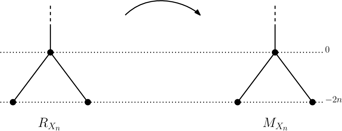
Therefore, the corresponding minimal graded subroot RXnR_{X_{n}} and the monotone subroot MXnM_{X_{n}} of XnX_{n} are shown in Figure 5.

Proof.

By Lemma 4.6, {Xn}n=1∞\{X_{n}\}^{\infty}_{n=1} has the wanted reduced delta sequence, see Section 2.4. Then the corresponding minimal graded root RXnR_{X_{n}} is constructed by using the recipe in Section 2.5. In this case, the monotone subroot MXnM_{X_{n}} is same with RXnR_{X_{n}} due to Section 2.6 and Theorem 3.2. ∎

Refer to caption
Figure 5. The minimal graded and monotone subroots of {Xn}n=1∞\{X_{n}\}^{\infty}_{n=1}.

4.3. Computations for {Yn=Σ(2n+1,3n+2,6n+1)}n=1∞\{Y_{n}=\Sigma(2n+1,3n+2,6n+1)\}^{\infty}_{n=1}

Since the lattice point realizing the dd-invariant of {Yn}n=1∞\{Y_{n}\}^{\infty}_{n=1} is same with one of {Xn}n=1∞\{X_{n}\}^{\infty}_{n=1}, by [KŞ20, Lemma 4.6, Theorem 1.2], the values of aa and bb has the same formula but the values of x,yx,y and zz are different. Note that d⁡(Yn)=−2​nd(Y_{n})=-2n for n≥1n\geq 1.

Lemma 4.8.

For {Yn}n=1∞\{Y_{n}\}^{\infty}_{n=1}, the positions of terminal cohomology classes k1k_{1} and k2k_{2} of good full paths for {Yn}n=1∞\{Y_{n}\}^{\infty}_{n=1} in the Laufer sequence are

a=x+(n−1)​zandb=y+(n−1)​z.\displaystyle a=x+(n-1)z\ \ \text{and}\ \ b=y+(n-1)z.

Thus a,b∈SYn.a,b\in S_{Y_{n}}.

Proof.

Notice that x=(2​n+1)​(3​n+2)x=(2n+1)(3n+2), y=(2​n+1)​(6​n+1)y=(2n+1)(6n+1) and z=(3​n+2)​(6​n+1)z=(3n+2)(6n+1) for {Yn}n=1∞\{Y_{n}\}^{\infty}_{n=1}. The proof of lemma is identical with Lemma 4.4 with exception of values of x,yx,y and zz. ∎

Next we define two special packed sequences for {Yn}n=1∞\{Y_{n}\}^{\infty}_{n=1}:

θ𝐤\displaystyle\mathbf{\theta_{k}} =[(𝟏+𝟑​𝐤)​𝐱+(𝐧−𝟏−𝐤)​𝐳]​ for all ​k∈{0,1,…,n−1},\displaystyle=\mathbf{[(1+3k)x+(n-1-k)z]}\text{ for all }k\in\{0,1,\ldots,n-1\},
ωℓ\displaystyle\mathbf{\omega_{\ell}} =[(𝟏+𝟑​ℓ)​𝐲+(𝐧−𝟏−𝟐​ℓ)​𝐳]​ for all ​ℓ∈{1,2,…,⌊n−12⌋}.\displaystyle=\mathbf{[(1+3\ell)y+(n-1-2\ell)z]}\text{ for all }\ell\in\left\{1,2,\ldots,\left\lfloor\frac{n-1}{2}\right\rfloor\right\}.

By Lemma 4.3, it is clear that θ𝐤\mathbf{\theta_{k}} contains n−kn-k elements and ωℓ\mathbf{\omega_{\ell}} contains n−2​ℓn-2\ell elements.

Lemma 4.9.

For the packed sequences θ𝐤\mathbf{\theta_{k}} and ωℓ\mathbf{\omega_{\ell}}, the following facts hold:

  1. (1)

    θ𝐤𝟏<θ𝐤𝟐\mathbf{\theta_{k_{1}}}<\mathbf{\theta_{k_{2}}} for all k1,k2∈{0,1,…,n−1}k_{1},k_{2}\in\{0,1,\dots,n-1\} with k1<k2k_{1}<k_{2}.

  2. (2)

    ωℓ𝟐<ωℓ𝟏\mathbf{\omega_{\ell_{2}}}<\mathbf{\omega_{\ell_{1}}} for all ℓ1,ℓ2∈{1,2,…,⌊n−12⌋}\ell_{1},\ell_{2}\in\left\{1,2,\dots,\left\lfloor\frac{n-1}{2}\right\rfloor\right\} with ℓ1<ℓ2\ell_{1}<\ell_{2}.

  3. (3)

    a≤θ𝐤<ba\leq\mathbf{\theta_{k}}<b for all k∈{0,1,…,n−1}k\in\{0,1,\dots,n-1\}.

  4. (4)

    a<ωℓ<ba<\mathbf{\omega_{\ell}}<b for all ℓ∈{1,2,…,⌊n−12⌋}\ell\in\left\{1,2,\dots,\left\lfloor\frac{n-1}{2}\right\rfloor\right\}.

  5. (5)

    θ𝐧−ℓ−𝟏<ωℓ<θ𝐧−ℓ\mathbf{\theta_{n-\ell-1}}<\mathbf{\omega_{\ell}}<\mathbf{\theta_{n-\ell}} for all ℓ∈{1,2,…,⌊n−12⌋}\ell\in\left\{1,2,\dots,\left\lfloor\frac{n-1}{2}\right\rfloor\right\}.

Proof.

We consider the proof case by case.

  1. (1)

    There is nothing to prove when n=1n=1. Assume n≥2n\geq 2. It suffices to show that θ𝐤<θ𝐤+𝟏\mathbf{\theta_{k}}<\mathbf{\theta_{k+1}} for all k∈{0,1,…,n−2}k\in\{0,1,\dots,n-2\}. To check the latter it is enough to compare the initial elements of the respective packed sequences, so the claim is equivalent to showing (1+3​k)​x+(n−1−k)​z<(1+3​(k+1))​x+(n−1−k)​z(1+3k)x+(n-1-k)z<(1+3(k+1))x+(n-1-k)z, which is true because 3​x−z=6​n+4>03x-z=6n+4>0 for all nn.

  2. (2)

    The claim is trivial when n≤4n\leq 4, so assume n≥5n\geq 5. It suffices to show that ωℓ+𝟏<ωℓ\mathbf{\omega_{\ell+1}}<\mathbf{\omega_{\ell}} for all ℓ∈{1,2,…,⌊n−12⌋−1}\ell\in\left\{1,2,\dots,\lfloor\frac{n-1}{2}\rfloor-1\right\}. To prove the latter we again compare the initial elements and show (1+3​(ℓ+1))​y+(n−1−2​(ℓ+1))​z<(1+3​ℓ)​y+(n−2−2​ℓ)​z(1+3(\ell+1))y+(n-1-2(\ell+1))z<(1+3\ell)y+(n-2-2\ell)z. This inequality is equivalent to 3​y−2​z<03y-2z<0 which is true because 3​y−2​z=−(6​n+1)3y-2z=-(6n+1).

  3. (3)

    Notice that aa is the initial element of θ0\theta_{0}, hence by part (1) we have a≤θ𝐤a\leq\mathbf{\theta_{k}} for all kk. To prove the rest, observe that θ𝐧−𝟏\mathbf{\theta_{n-1}} consists of a single element namely (1+3​(n−1))​x(1+3(n-1))x, so it suffices to show this element is stricly less than bb. The required inequality is (1+3​(n−1))​x<y+(n−1)​z(1+3(n-1))x<y+(n-1)z, which is equivalent to n⁡(y−2​x−1)+x+1>0n(y-2x-1)+x+1>0 by the identity (4.1). The latter is true for all nn because y−2​x=−(6​n+3)y-2x=-(6n+3) and x=6​n2+7​n+2x=6n^{2}+7n+2.

  4. (4)

    By part (2), we need to see that the last element of ω𝟏\mathbf{\omega_{1}} is less than bb, i.e., (n−3)​x+(n+1)​y<y+(n−1)​z(n-3)x+(n+1)y<y+(n-1)z. Using the identity (4.1), it suffices to show that 2​x−y+1−n>02x-y+1-n>0. It is true for all nn because 2​x−y=6​n+32x-y=6n+3. For the rest it is enough to verify that aa is less than the initial element of ω⌊𝐧−𝟏𝟐⌋\mathbf{\omega_{\left\lfloor\frac{n-1}{2}\right\rfloor}}, i.e., we need to have x+(n−1)​z<(1+3​⌊n−12⌋)​y+(n−1−2​⌊n−12⌋)​zx+(n-1)z<\left(1+3\left\lfloor\frac{n-1}{2}\right\rfloor\right)y+\left(n-1-2\left\lfloor\frac{n-1}{2}\right\rfloor\right)z. It is equivalent to showing that y−x+⌊n−12⌋​(3​y−2​z)>0y-x+\left\lfloor\frac{n-1}{2}\right\rfloor(3y-2z)>0 for all nn. This is true since y−x=(2​n+1)​(3​n−1)y-x=(2n+1)(3n-1) and 3​y−2​x=−(6​n+1)3y-2x=-(6n+1).

  5. (5)

    We compare the initial elements of relevant packed sequences. We show that the inequalities (1+3​(n−ℓ−1))​x+ℓ​z<(1+3​ℓ)​y+(n−1−2​ℓ)​z(1+3(n-\ell-1))x+\ell z<(1+3\ell)y+(n-1-2\ell)z and (1+3​ℓ)​y+(n−1−2​ℓ)​z<(1+3​(n−ℓ))​x+(ℓ−1)​z(1+3\ell)y+(n-1-2\ell)z<(1+3(n-\ell))x+(\ell-1)z both hold. Using the identity (4.1), we reduce the former inequality n⁡(y−2​x−1)+x+3​ℓ+1>0n(y-2x-1)+x+3\ell+1>0. Since y−2​x=−(6​n+3)y-2x=-(6n+3) and x=6​n2+7​n+2x=6n^{2}+7n+2, this inequality is true for all nn. Again by the identity (4.1), we transform the latter inequality to n⁡(2​x−y+1)+x−y−3​ℓ>0n(2x-y+1)+x-y-3\ell>0 which is true for all nn since 2​x−y=6​n+32x-y=6n+3 and x−y=−6​n2−n+1x-y=-6n^{2}-n+1.

∎

Lemma 4.10.

Any element in SYn∩[a,b)S_{Y_{n}}\cap[a,b) must belong to one of the packed sequences θ𝐤\mathbf{\theta_{k}} for some k∈{0,1,…,n−1}k\in\{0,1,\ldots,n-1\} or ωℓ\mathbf{\omega_{\ell}} for some ℓ∈{1,2,…,⌊n−12⌋}\ell\in\left\{1,2,\ldots,\lfloor\frac{n-1}{2}\rfloor\right\}.

Proof.

Assume for a contradiction that there exists another element d∈SYn∩[a,b)d\in S_{Y_{n}}\cap[a,b). Without loss of generality suppose that dd is an initial element of a packed sequence. We consider the following two cases.

Case I. d=f​x+h​zd=fx+hz where 0≤h≤n−10\leq h\leq n-1.

We can re-parametrize dd as d=f​x+(n−1−k)​zd=fx+(n-1-k)z for k∈{0,1,…,n−1}k\in\{0,1,\dots,n-1\}. We will prove that dd must be the initial element of θ𝐤\mathbf{\theta_{k}}. By Lemma 4.9, we have a≤d<ba\leq d<b, so

x+(n−1)​z≤f​x+(n−1−k)​z<y+(n−1)​z,\displaystyle x+(n-1)z\leq fx+(n-1-k)z<y+(n-1)z,

which implies

0≤(f−1)​x−k​z<y−x.\displaystyle 0\leq(f-1)x-kz<y-x.

Dividing by xx, we get

0≤f−1−k​zx<yx−1.\displaystyle 0\leq f-1-k\frac{z}{x}<\frac{y}{x}-1.

Notice that yx<2\frac{y}{x}<2 for all nn, hence

0≤f−1−k​zx<1.\displaystyle 0\leq f-1-k\frac{z}{x}<1.

We write zx=3−22​n+1\frac{z}{x}=3-\frac{2}{2n+1} and re-arrange the terms as follows

−2​k2​n+1≤f−1−3​k<1−2​k2​n+1.\displaystyle-\frac{2k}{2n+1}\leq f-1-3k<1-\frac{2k}{2n+1}.

Now as 0≤2​k2​n+1<10\leq\frac{2k}{2n+1}<1, we have

−1<f−1+3​k<1\displaystyle-1<f-1+3k<1

The only integer ff satisfying the above inequality is f=1+3​kf=1+3k.

Case II. d=g​y+h​zd=gy+hz where 0≤h≤n−10\leq h\leq n-1.

We will follow a similar strategy as in Case I and show that dd is the initial element of the packed sequence ωℓ\mathbf{\omega_{\ell}} for some ℓ\ell. Write h=n−1−kh=n-1-k for k∈{0,1,…,n−1}k\in\{0,1,\dots,n-1\}. Since aa is the initial element of θ𝟎\mathbf{\theta_{0}} and dd is not of this form, by Lemma 4.9, we have the strict inequality a<d<ba<d<b, so

x+(n−1)​z<g​y+(n−1−k)​z<y+(n−1)​z.\displaystyle x+(n-1)z<gy+(n-1-k)z<y+(n-1)z.

Subtract y+(n−1)​zy+(n-1)z to get

x−y<(g−1)​y−k​z<0.\displaystyle x-y<(g-1)y-kz<0.

Dividing by yy we obtain

xy−1<g−1−k​zy<0.\displaystyle\frac{x}{y}-1<g-1-k\frac{z}{y}<0.

Plug in xy=3​n+26​n+1=12+312​n+2\frac{x}{y}=\frac{3n+2}{6n+1}=\frac{1}{2}+\frac{3}{12n+2} and zy=3​n+22​n+1=32+14​n+2\frac{z}{y}=\frac{3n+2}{2n+1}=\frac{3}{2}+\frac{1}{4n+2} and re-arranging we have

−12+312​n+2+k4​n+2<g−1−3​k2<k4​n+2\displaystyle-\frac{1}{2}+\frac{3}{12n+2}+\frac{k}{4n+2}<g-1-\frac{3k}{2}<\frac{k}{4n+2}

Since 0≤k≤n−10\leq k\leq n-1, we find

−14<g−1−3​k2<14\displaystyle-\frac{1}{4}<g-1-\frac{3k}{2}<\frac{1}{4}

We see that when kk is odd the above inequality has not an integer solution for gg. When kk is even, we can write k=2​ℓk=2\ell for ℓ∈{1,2,…,⌊n−12⌋}\ell\in\left\{1,2,\dots,\lfloor\frac{n-1}{2}\rfloor\right\} and g=1+3​ℓg=1+3\ell as required. ∎

Using preceding lemmas, we precisely describe all elements lying in SYn∩[a,b]S_{Y_{n}}\cap[a,b].

Lemma 4.11.

As an ordered set, SYn∩[a,b]S_{Y_{n}}\cap[a,b] is given by the following sequences and elements

θ𝟎,θ𝟏,…,θ⌊𝐧𝟐⌋,ω⌊𝐧−𝟏𝟐⌋,θ⌊𝐧𝟐⌋+𝟏,ω⌊𝐧−𝟏𝟐⌋−𝟏,…,θ𝐧−𝟐,ω𝟏,θ𝐧−𝟏,b\mathbf{\theta_{0}},\mathbf{\theta_{1}},\dots,\mathbf{\theta_{\left\lfloor\frac{n}{2}\right\rfloor}},\mathbf{\omega_{\left\lfloor\frac{n-1}{2}\right\rfloor}},\mathbf{\theta_{\left\lfloor\frac{n}{2}\right\rfloor+1}},\mathbf{\omega_{\left\lfloor\frac{n-1}{2}\right\rfloor-1}},\dots,\mathbf{\theta_{n-2}},\mathbf{\omega_{1}},\mathbf{\theta_{n-1}},b

Proof.

The proof follows the combination of Lemma 4.4, Lemma 4.3, Lemma 4.9, and Lemma 4.10. ∎

Lemma 4.12.

The complementary packed sequences satisfy the following inequalities:

  1. (1)

    θ𝐤−𝟏<N0−θ𝐧−𝐤<θ𝐤\mathbf{\theta_{k-1}}<N_{0}-\mathbf{\theta_{n-k}}<\mathbf{\theta_{k}} for all k∈{1,2,…,n−1}k\in\{1,2,\dots,n-1\},

  2. (2)

    θℓ−𝟏<N0−ωℓ<θℓ\mathbf{\theta_{\ell-1}}<N_{0}-\mathbf{\omega_{\ell}}<\mathbf{\theta_{\ell}} for all ℓ∈{1,2,…,⌊n−12⌋},\ell\in\left\{1,2,\dots,\lfloor\frac{n-1}{2}\rfloor\right\},

Proof.

Since p​q​r=p​zpqr=pz and p=2​n+1p=2n+1, using the identity (4.1), we write

(4.2) N0=(2​n−1)​x+(2​n−1)​y−2​n\displaystyle N_{0}=(2n-1)x+(2n-1)y-2n
  1. (1)

    We compare the initial elements of relevant packed sequences. We show that the inequalities (1+3​(k−1))​x+(n−k)​z<N0−(1+3​(n−k))​x−(k−1)​z(1+3(k-1))x+(n-k)z<N_{0}-(1+3(n-k))x-(k-1)z and N0−(1+3​(n−k))​x−(k−1)​z<(1+3​k)​x+(n−k−1)​zN_{0}-(1+3(n-k))x-(k-1)z<(1+3k)x+(n-k-1)z both hold. The former inequality is a consequence following equalities:

    OPENN0−((1+3​(n−k))​x+(k−1)​z+1+3​(k−1))​x+(n−k)​z)\displaystyle N_{0}-\left((1+3(n-k))x+(k-1)z+1+3(k-1))x+(n-k)z\right)
    =N0−((3​n−1)​x+(n−1)​z)\displaystyle=N_{0}-\left((3n-1)x+(n-1)z\right)
    =(4.1)​N0−((4​n−2)​x+(n−1)​y−n+1)\displaystyle{\overset{\eqref{xyz}}{=}}N_{0}-\left((4n-2)x+(n-1)y-n+1\right)
    =(4.2)​(2​n−1)​x+(2​n−1)​y−2​n−((4​n−2)​x+(n−1)​y−n+1)\displaystyle{\overset{\eqref{N0}}{=}}(2n-1)x+(2n-1)y-2n-\left((4n-2)x+(n-1)y-n+1\right)
    =n⁡(y−2​x)+x−n−1>0\displaystyle=n(y-2x)+x-n-1>0

    This is true since y−2​x=−(6​n+3)y-2x=-(6n+3) and x=6​n2+7​n+2x=6n^{2}+7n+2. We can derive the second inequality for all nn since 2​x−y=6​n+12x-y=6n+1:

    (1+3​(n−k))​x+(k−1)​z+(1+3​k)​x+(n−k−1)​z−N0\displaystyle(1+3(n-k))x+(k-1)z+(1+3k)x+(n-k-1)z-N_{0}
    =(3​n+2)​x+(n−2)​z−N0\displaystyle=(3n+2)x+(n-2)z-N_{0}
    =(4.1)​4​n​x+n​y−2​y+n+2−N0\displaystyle{\overset{\eqref{xyz}}{=}}4nx+ny-2y+n+2-N_{0}
    =(4.2)​4​n​x+n​y−2​y+n+2−((2​n−1)​x+(2​n−1)​y−2​n)\displaystyle{\overset{\eqref{N0}}{=}}4nx+ny-2y+n+2-\left((2n-1)x+(2n-1)y-2n\right)
    =n⁡(2​x−y)+x+y+2>0\displaystyle=n(2x-y)+x+y+2>0
  2. (2)

    In this case, we follow the same strategy by comparing the initial elements of our sequences. It suffices to prove that the inequalities (1+3​(ℓ−1))​x+(n−ℓ)​z<N0−(1+3​ℓ)​y−(n−1−2​ℓ)​z(1+3(\ell-1))x+(n-\ell)z<N_{0}-(1+3\ell)y-(n-1-2\ell)z and N0−(1+3​ℓ)​y−(n−1−2​ℓ)​z<(1+3​ℓ)​x+(n−1−ℓ)​zN_{0}-(1+3\ell)y-(n-1-2\ell)z<(1+3\ell)x+(n-1-\ell)z are true for all nn. To see the first equality, we do the following calculations:

    OPENN0−((1+3​ℓ)​y+(n−1−2​ℓ)​z+3​(ℓ−1))​x+(n−ℓ)​z)\displaystyle N_{0}-\left((1+3\ell)y+(n-1-2\ell)z+3(\ell-1))x+(n-\ell)z\right)
    OPEN=N0−(3​(ℓ−1))​x+(1+3​ℓ)​y+(2​n−3​ℓ−1)​z)\displaystyle=N_{0}-\left(3(\ell-1))x+(1+3\ell)y+(2n-3\ell-1)z\right)
    =(4.1)​N0−((2​n−3)​x+2​n​y−2​n+3​ℓ+1)\displaystyle{\overset{\eqref{xyz}}{=}}N_{0}-\left((2n-3)x+2ny-2n+3\ell+1\right)
    =(4.2)​(2​n−1)​x+(2​n−1)​y−2​n−((2​n−3)​x+2​n​y−2​n+3​ℓ+1)\displaystyle{\overset{\eqref{N0}}{=}}(2n-1)x+(2n-1)y-2n-\left((2n-3)x+2ny-2n+3\ell+1\right)
    =2​x−y−3​ℓ−1>0\displaystyle=2x-y-3\ell-1>0

    The latter one is true since 2​x−y=6​n+32x-y=6n+3. The last inequality also holds because:

    (1+3​ℓ)​x+(n−1−ℓ)​z+(1+3​ℓ)​y+(n−1−2​ℓ)​z−N0\displaystyle(1+3\ell)x+(n-1-\ell)z+(1+3\ell)y+(n-1-2\ell)z-N_{0}
    =(1+3​ℓ)​x+(1+3​ℓ)​y+(2​n−2−3​ℓ)​z−N0\displaystyle=(1+3\ell)x+(1+3\ell)y+(2n-2-3\ell)z-N_{0}
    =(4.1)​(2​n−1)​x+(2​n−1)​y−2​n+2+3​ℓ−N0\displaystyle{\overset{\eqref{xyz}}{=}}(2n-1)x+(2n-1)y-2n+2+3\ell-N_{0}
    =(4.2)​(2​n−1)​x+(2​n−1)​y−2​n+2+3​ℓ−((2​n−1)​x+(2​n−1)​y−2​n)\displaystyle{\overset{\eqref{N0}}{=}}(2n-1)x+(2n-1)y-2n+2+3\ell-\left((2n-1)x+(2n-1)y-2n\right)
    =3​ℓ+2>0\displaystyle=3\ell+2>0

∎

Now we are able to list all elements inside XYn∩[a,b]X_{Y_{n}}\cap[a,b].

Lemma 4.13.

As an ordered set, the elements of XYn∩[a,b]X_{Y_{n}}\cap[a,b] are respectively given by the following sequences and elements. When nn is odd, we have

θ𝟎,N0−θ𝐧−𝟏,N0−ω𝟏,…,θ𝐧−𝟑𝟐,N0−θ𝐧+𝟏𝟐,N0−ω𝐧−𝟏𝟐,θ𝐧−𝟏𝟐,N0−θ𝐧−𝟏𝟐,ω𝐧−𝟏𝟐,θ𝐧+𝟏𝟐,N0−θ𝐧−𝟑𝟐,…,ω𝟏,θ𝐧−𝟏,N0−θ𝟎,b\mathbf{\theta_{0}},N_{0}-\mathbf{\theta_{n-1}},N_{0}-\mathbf{\omega_{1}},\dots,\mathbf{\theta_{\frac{n-3}{2}}},N_{0}-\mathbf{\theta_{\frac{n+1}{2}}},N_{0}-\mathbf{\omega_{\frac{n-1}{2}}},\mathbf{\theta_{\frac{n-1}{2}}},N_{0}-\mathbf{\theta_{\frac{n-1}{2}}},\newline \mathbf{\omega_{\frac{n-1}{2}}},\mathbf{\theta_{\frac{n+1}{2}}},N_{0}-\mathbf{\theta_{\frac{n-3}{2}}},\dots,\mathbf{\omega_{1}},\mathbf{\theta_{n-1}},N_{0}-\mathbf{\theta_{0}},b

For even values of nn, we also have

θ𝟎,N0−θ𝐧−𝟏,N0−ω𝟏,…,θ𝐧−𝟒𝟐,N0−θ𝐧+𝟐𝟐,N0−ω𝐧−𝟐𝟐,θ𝐧−𝟐𝟐,N0−θ𝐧𝟐,θ𝐧𝟐,N0−θ𝐧−𝟐𝟐,ω𝐧−𝟐𝟐,θ𝐧+𝟐𝟐,N0−θ𝐧−𝟒𝟐,…,ω𝟏,θ𝐧−𝟏,N0−θ𝟎,b\mathbf{\theta_{0}},N_{0}-\mathbf{\theta_{n-1}},N_{0}-\mathbf{\omega_{1}},\dots,\mathbf{\theta_{\frac{n-4}{2}}},N_{0}-\mathbf{\theta_{\frac{n+2}{2}}},N_{0}-\mathbf{\omega_{\frac{n-2}{2}}},\mathbf{\theta_{\frac{n-2}{2}}},N_{0}-\mathbf{\theta_{\frac{n}{2}}},\mathbf{\theta_{\frac{n}{2}}},\newline N_{0}-\mathbf{\theta_{\frac{n-2}{2}}},\mathbf{\omega_{\frac{n-2}{2}}},\mathbf{\theta_{\frac{n+2}{2}}},N_{0}-\mathbf{\theta_{\frac{n-4}{2}}},\dots,\mathbf{\omega_{1}},\mathbf{\theta_{n-1}},N_{0}-\mathbf{\theta_{0}},b

Proof.

Observe that the packed sequences ω𝐣\mathbf{\omega_{j}} and θ𝐧−𝐣\mathbf{\theta_{n-j}} are consecutive in XYn∩[a,b]X_{Y_{n}}\cap[a,b], so are their complementary packed sequences. The rest of the claim follows the combination of Lemma 4.11 and Lemma 4.12. ∎

Proposition 4.14.

For {Yn}n=1∞\{Y_{n}\}^{\infty}_{n=1}, the reduced delta sequences Δ~Yn\tilde{\Delta}_{Y_{n}} on [a,b][a,b] are respectively given following sequences. When nn is odd, we have

⟨n,−(n−1),n−1,…,−(n+1)2,n+12,−(n+1)2,n+12,…,−(n−1),n−1,−n,1⟩.\left\langle n,-(n-1),n-1,\ldots,\frac{-(n+1)}{2},\frac{n+1}{2},\frac{-(n+1)}{2},\frac{n+1}{2},\ldots,-(n-1),n-1,-n,1\right\rangle.

For even values of nn, we also have

⟨n,−(n−1),n−1,…,−(n+2)2,n+22,−n2,n2,−(n+2)2,n+22,…,−(n−1),n−1,−n,1⟩.\left\langle n,-(n-1),n-1,\ldots,\frac{-(n+2)}{2},\frac{n+2}{2},\frac{-n}{2},\frac{n}{2},\frac{-(n+2)}{2},\frac{n+2}{2},\ldots,-(n-1),n-1,-n,1\right\rangle.

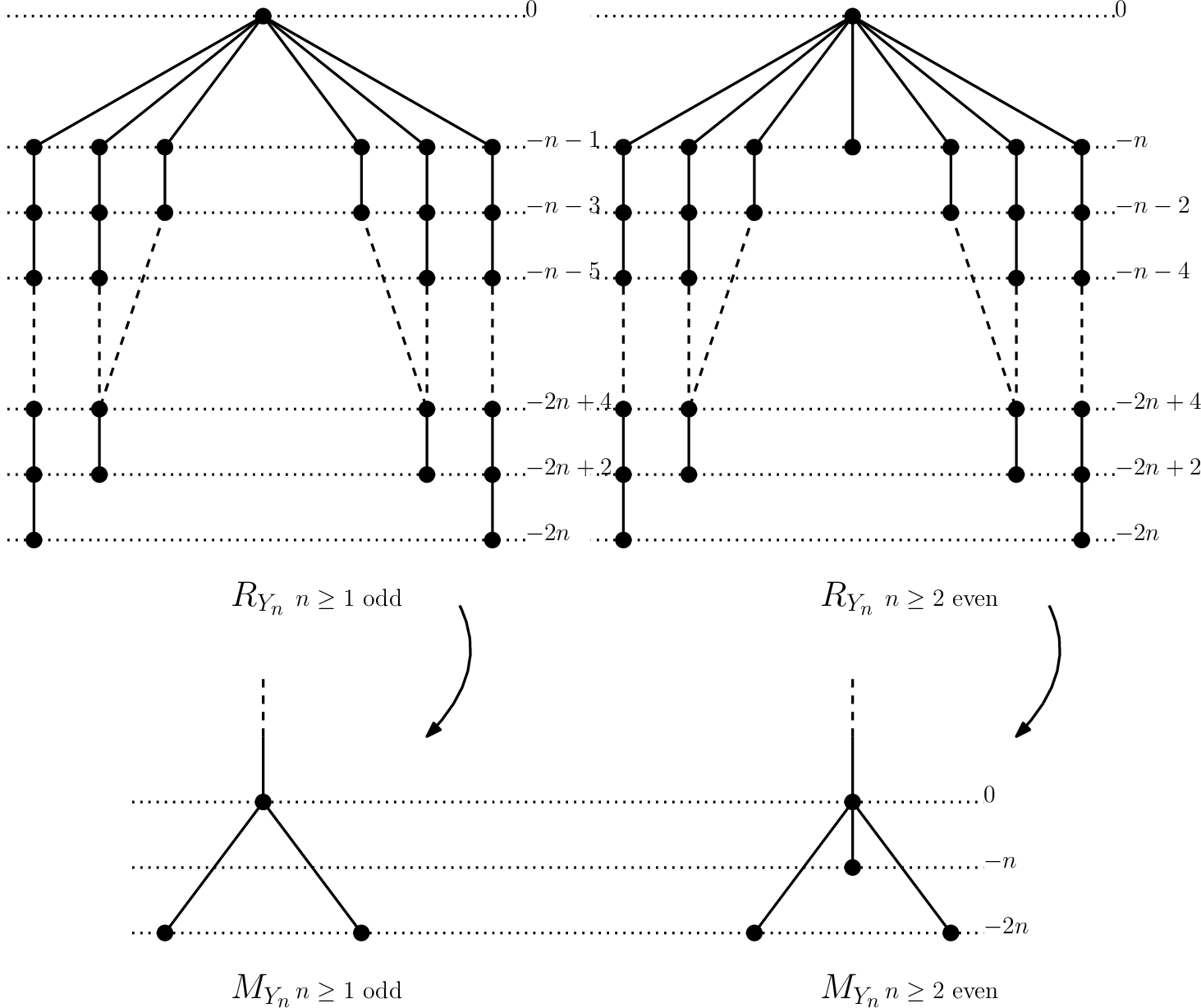
Therefore, the corresponding minimal graded subroots RYnR_{Y_{n}} and monotone subroots MYnM_{Y_{n}} of {Yn}n=1∞\{Y_{n}\}^{\infty}_{n=1} are shown in Figure 6.

Proof.

Recall that the sequences θ𝐤\mathbf{\theta_{k}} and N0−θ𝐤N_{0}-\mathbf{\theta_{k}} both contains n−kn-k elements and ωℓ\mathbf{\omega_{\ell}} and N0−ωℓN_{0}-\mathbf{\omega_{\ell}} both consist of n−2​ℓn-2\ell elements. So by Lemma 4.13, YnY_{n} has the reduced delta sequences as desired. Then the corresponding graded root RYnR_{Y_{n}} is constructed by passing to τ\tau sequences and using ingredients in Section 2.5. Finally, the monotone subroot MYnM_{Y_{n}} is extracted from RYnR_{Y_{n}} by following Section 2.6 and applying Theorem 3.2. ∎
Refer to caption
Figure 6. The minimal graded and monotone subroots of {Yn}n=1∞\{Y_{n}\}^{\infty}_{n=1}.

4.4. Computations for {Zn=Σ(2n+1,3n+1,6n+5)}n=1∞\{Z_{n}=\Sigma(2n+1,3n+1,6n+5)\}^{\infty}_{n=1}

We know that the lattice point realizing the dd-invariant of {Zn}n=1∞\{Z_{n}\}^{\infty}_{n=1} is same with one of {Xn}n=1∞\{X_{n}\}^{\infty}_{n=1} or {Yn}n=1∞\{Y_{n}\}^{\infty}_{n=1}, by [KŞ20, Lemma 4.6, Theorem 1.2], the values of aa and bb remain same except the values of x,yx,y and zz. Note that d⁡(Zn)=−2​nd(Z_{n})=-2n for n≥1n\geq 1.

Lemma 4.15.

For {Zn}n=1∞\{Z_{n}\}^{\infty}_{n=1}, the positions of terminal cohomology classes k1k_{1} and k2k_{2} of good full paths for {Zn}n=1∞\{Z_{n}\}^{\infty}_{n=1} in the Laufer sequence are

a=x+(n−1)​zandb=y+(n−1)​z.\displaystyle a=x+(n-1)z\ \ \text{and}\ \ b=y+(n-1)z.

Thus a,b∈SYn.a,b\in S_{Y_{n}}.

Proof.

For for {Zn}n=1∞\{Z_{n}\}^{\infty}_{n=1}, we remark that x=(2​n+1)​(3​n+1)x=(2n+1)(3n+1), y=(2​n+1)​(6​n+5)y=(2n+1)(6n+5) and z=(3​n+1)​(6​n+5)z=(3n+1)(6n+5) . The proof of lemma is identical with Lemma 4.4 or Lemma 4.8 by respecting new values of x,yx,y and zz. ∎

We introduce two packed sequences for {Zn}n=1∞\{Z_{n}\}^{\infty}_{n=1}:

η𝐤\displaystyle\mathbf{\eta_{k}} =[(𝟐+𝟑​𝐤)​𝐱+(𝐧−𝟏−𝐤)​𝐳]​ for all ​k∈{0,1,…,n−1},\displaystyle=\mathbf{[(2+3k)x+(n-1-k)z]}\text{ for all }k\in\{0,1,\ldots,n-1\},
ξℓ\displaystyle\mathbf{\xi_{\ell}} =[(−𝟏+𝟑​ℓ)​𝐲+(𝐧−𝟐​ℓ)​𝐳]​ for all ​ℓ∈{1,2,…,⌊n2⌋}.\displaystyle=\mathbf{[(-1+3\ell)y+(n-2\ell)z]}\text{ for all }\ell\in\left\{1,2,\ldots,\left\lfloor\frac{n}{2}\right\rfloor\right\}.

Lemma 4.3 indicates that η𝐤\mathbf{\eta_{k}} contains n−kn-k elements and ξℓ\mathbf{\xi_{\ell}} contains n+1−2​ℓn+1-2\ell elements.

Lemma 4.16.

For the packed sequences η𝐤\mathbf{\eta_{k}} and ξℓ\mathbf{\xi_{\ell}}, the following facts hold:

  1. (1)

    η𝐤𝟐<η𝐤𝟏\mathbf{\eta_{k_{2}}}<\mathbf{\eta_{k_{1}}} for all k1,k2∈{0,1,…,n−1}k_{1},k_{2}\in\{0,1,\dots,n-1\} with k1<k2k_{1}<k_{2}.

  2. (2)

    ξℓ𝟏<ξℓ𝟐\mathbf{\xi_{\ell_{1}}}<\mathbf{\xi_{\ell_{2}}} for all ℓ1,ℓ2∈{1,2,…,⌊n2⌋}\ell_{1},\ell_{2}\in\left\{1,2,\dots,\left\lfloor\frac{n}{2}\right\rfloor\right\} with ℓ1<ℓ2\ell_{1}<\ell_{2}.

  3. (3)

    a<η𝐤<ba<\mathbf{\eta_{k}}<b for all k∈{0,1,…,n−1}k\in\{0,1,\dots,n-1\}.

  4. (4)

    a<ξℓ<ba<\mathbf{\xi_{\ell}}<b for all ℓ∈{1,2,…,⌊n2⌋}\ell\in\left\{1,2,\dots,\left\lfloor\frac{n}{2}\right\rfloor\right\}.

  5. (5)

    ξℓ<η𝐧−ℓ<ξℓ+𝟏\mathbf{\xi_{\ell}}<\mathbf{\eta_{n-\ell}}<\mathbf{\xi_{\ell+1}} for all ℓ∈{1,2,…,⌊n2⌋−1}\ell\in\left\{1,2,\dots,\left\lfloor\frac{n}{2}\right\rfloor-1\right\}.

Proof.

We consider the proof case by case.

  1. (1)

    Suppose n≥2n\geq 2 since there is nothing to show when n=1n=1. It is enough to prove that η𝐤+𝟏<η𝐤\mathbf{\eta_{k+1}}<\mathbf{\eta_{k}} for all k∈{0,1,…,n−2}k\in\{0,1,\dots,n-2\}. To verify the latter inequality, it suffices to compare the initial elements of the respective packed sequences, i.e., (2+3​(k+1))​x+(n−2−k)​z<(2+3​k)​x+(n−1−k)​z(2+3(k+1))x+(n-2-k)z<(2+3k)x+(n-1-k)z. This is true because z−3​x=6​n+2>0z-3x=6n+2>0 for all nn.

  2. (2)

    The claim is straightforward when n≤2n\leq 2, thus assume n≥3n\geq 3. It suffices to prove that ξℓ<ξℓ+𝟏\mathbf{\xi_{\ell}}<\mathbf{\xi_{\ell+1}} for all ℓ∈{1,2,…,⌊n2⌋}\ell\in\left\{1,2,\dots,\lfloor\frac{n}{2}\rfloor\right\}. To show this inequality, we again compare the initial elements and show (−1+3​ℓ)​y+(n−2​ℓ)​z<(−1+3​(ℓ+1))​y+(n−2​(ℓ+1))​z(-1+3\ell)y+(n-2\ell)z<(-1+3(\ell+1))y+(n-2(\ell+1))z. This inequality is equivalent to 2​z−3​y<02z-3y<0 which holds for all nn since 3​y−2​z=6​n+53y-2z=6n+5.

  3. (3)

    In part (1), we see that η𝐤\mathbf{\eta_{k}} is decreasing. Thus, it is enough to compare the initial element of η𝐧−𝟏\mathbf{\eta_{n-1}} with aa and the initial element of η𝟎\mathbf{\eta_{0}} with bb. For the former inequality, we need to show that x+(n−1)​z<(2+3​(n−1))​xx+(n-1)z<(2+3(n-1))x which is equivalent to n⁡(2​x−y)+y+n−1>0n(2x-y)+y+n-1>0 by the identity (4.1). As 2​x−y=−(6​n+3)2x-y=-(6n+3) and y=12​n2+16​n+5y=12n^{2}+16n+5 this inequality holds for all nn. To prove the rest, the required inequality is 2​x+(n−1)​z<y+(n−1)​z2x+(n-1)z<y+(n-1)z, which is clearly true since y−2​x=6​n+3>0y-2x=6n+3>0 for all nn.

  4. (4)

    The part (2) indicates that ξℓ\mathbf{\xi_{\ell}} is increasing, so we follow the strategy of the previous part by showing that two inequalities a<ξ𝟏a<\mathbf{\xi_{1}} and ξ⌊𝐧𝟐⌋<b\mathbf{\xi_{\left\lfloor\frac{n}{2}\right\rfloor}}<b hold. Again, we compare the initial elements of required packed sequences. To verify the former inequality, we need to see that x+(n−1)​z<2​y+(n−2)​zx+(n-1)z<2y+(n-2)z. It reduces to 2​x−y−1<02x-y-1<0 by using the identity (4.1), which is true for all nn since 2​x−y=−(6​n+3)2x-y=-(6n+3). To complete the proof of this case, now we need to prove that bb is greater than the initial element of ξ⌊𝐧𝟐⌋\mathbf{\xi_{\left\lfloor\frac{n}{2}\right\rfloor}}. The wanted inequality is (−1+3​⌊n2⌋)​y+(n−2​⌊n2⌋)​z<y+(n−1)​z\left(-1+3\left\lfloor\frac{n}{2}\right\rfloor\right)y+\left(n-2\left\lfloor\frac{n}{2}\right\rfloor\right)z<y+(n-1)z. We rewrite it as 2​y−z+⌊n2⌋​(2​z−3​y)>02y-z+\left\lfloor\frac{n}{2}\right\rfloor(2z-3y)>0. This is true for all nn since 2​z−3​y=−(6​n+5)2z-3y=-(6n+5) and 2​y−z=(6​n+5)​(n+1)2y-z=(6n+5)(n+1).

  5. (5)

    We compare the initial elements of packed sequences ξℓ,η𝐧−ℓ\mathbf{\xi_{\ell}},\mathbf{\eta_{n-\ell}} and ξℓ+𝟏\mathbf{\xi_{\ell+1}} by showing that the inequalities (−1+3​ℓ)​y+(n−2​ℓ)​z<(2+3​(n−ℓ))​x+(ℓ−1)​z(-1+3\ell)y+(n-2\ell)z<(2+3(n-\ell))x+(\ell-1)z and (2+3​(n−ℓ))​x+(ℓ−1)​z<(−1+3​(ℓ+1))​y+(n−2​(ℓ+1))​z(2+3(n-\ell))x+(\ell-1)z<(-1+3(\ell+1))y+(n-2(\ell+1))z both hold. Using the identity (4.1), we reduce the former inequality n⁡(2​x−y)+x+n−3​ℓ+1>0n(2x-y)+x+n-3\ell+1>0. Since 2​x−y=−(6​n+3)2x-y=-(6n+3) and x=6​n2+5​n+1x=6n^{2}+5n+1, it turns out that 3​n−3​ℓ+2>03n-3\ell+2>0 which is true for all nn. Again by the identity (4.1), we transform the latter inequality to n⁡(y−2​x)+y−3​x−n+3​ℓ+1>0n(y-2x)+y-3x-n+3\ell+1>0. Since y−2​x=6​n+3y-2x=6n+3 and y−3​x=−6​n2+n+2y-3x=-6n^{2}+n+2, it is equivalent to 3​n+3​ℓ+3>03n+3\ell+3>0. It clearly holds for all nn.

∎

Lemma 4.17.

Any element in SZn∩(a,b)S_{Z_{n}}\cap(a,b) must belong to one of the packed sequences η𝐤\mathbf{\eta_{k}} for some k∈{0,1,…,n−1}k\in\{0,1,\ldots,n-1\} or ξℓ\mathbf{\xi_{\ell}} for some ℓ∈{1,2,…,⌊n2⌋}\ell\in\left\{1,2,\ldots,\lfloor\frac{n}{2}\rfloor\right\}.

Proof.

We suppose for a contradiction that there exists another element e∈SZn∩(a,b)e\in S_{Z_{n}}\cap(a,b). Assume without loss of generality that ee is an initial element of a packed sequence. We split the proof into two cases.

Case I. e=f​x+h​ze=fx+hz where 0≤h≤n−10\leq h\leq n-1.

The integer ee can be re-parametrized as e=f​x+(n−1−k)​ze=fx+(n-1-k)z for k∈{0,1,…,n−1}k\in\{0,1,\dots,n-1\}. In this case, we will verify that ee must be the initial element of η𝐤\mathbf{\eta_{k}}. By Lemma 4.16, we have a<e<ba<e<b, so

x+(n−1)​z<f​x+(n−1−k)​z<y+(n−1)​z,\displaystyle x+(n-1)z<fx+(n-1-k)z<y+(n-1)z,

which is equivalent to

0<(f−1)​x−k​z<y−x.\displaystyle 0<(f-1)x-kz<y-x.

Dividing all sides by xx, we obtain

0<f−1−k​zx<yx−1.\displaystyle 0<f-1-k\frac{z}{x}<\frac{y}{x}-1.

Notice that yx<3\frac{y}{x}<3 for all nn, thus

0<f−1−k​zx<2.\displaystyle 0<f-1-k\frac{z}{x}<2.

Here, zx=3+22​n+1\frac{z}{x}=3+\frac{2}{2n+1} which implies that

2​k2​n+1<f−1−3​k<2+2​k2​n+1.\displaystyle\frac{2k}{2n+1}<f-1-3k<2+\frac{2k}{2n+1}.

Since 0≤2​k2​n+1<10\leq\frac{2k}{2n+1}<1, we find that

0<f−1−3​k<2\displaystyle 0<f-1-3k<2

Clearly, the only integer solution satisfying the above inequality is f=2+3​kf=2+3k as we desired.

Case II. e=g​y+h​ze=gy+hz where 1≤h≤n1\leq h\leq n.

Likewise in Case I, we show that ee is the initial element of the packed sequence ωℓ\mathbf{\omega_{\ell}} for some ℓ\ell. Write h=n−kh=n-k for k∈{1,2,…,n}k\in\{1,2,\dots,n\}. By Lemma 4.9, we know tht a<e<ba<e<b, thus

x+(n−1)​z<g​y+(n−k)​z<y+(n−1)​z.\displaystyle x+(n-1)z<gy+(n-k)z<y+(n-1)z.

Subtract y+(n−1)​zy+(n-1)z from all sides to get

x−y<(g−1)​y+(1−k)​z<0.\displaystyle x-y<(g-1)y+(1-k)z<0.

Dividing by yy, we see that

xy−1<g−1+(1−k)​zy<0.\displaystyle\frac{x}{y}-1<g-1+(1-k)\frac{z}{y}<0.

Now plug in xy=3​n+16​n+5=12−312​n+10\frac{x}{y}=\frac{3n+1}{6n+5}=\frac{1}{2}-\frac{3}{12n+10} and zy=3​n+12​n+1=32−14​n+2\frac{z}{y}=\frac{3n+1}{2n+1}=\frac{3}{2}-\frac{1}{4n+2} and re-arrange the terms so that

−2−312​n+10+14​n+2−k4​n+2<g−1−3​k2<−32+14​n+2−k4​n+2\displaystyle-2-\frac{3}{12n+10}+\frac{1}{4n+2}-\frac{k}{4n+2}<g-1-\frac{3k}{2}<-\frac{3}{2}+\frac{1}{4n+2}-\frac{k}{4n+2}

Since 0≤k≤n0\leq k\leq n, we find that

−94<g−1−3​k2<−74\displaystyle-\frac{9}{4}<g-1-\frac{3k}{2}<-\frac{7}{4}

When kk is odd, clearly, there is no integer solution for gg. However, when kk is even, we may write k=2​ℓk=2\ell for ℓ∈{1,2,…,⌊n2⌋}\ell\in\left\{1,2,\dots,\lfloor\frac{n}{2}\rfloor\right\} and thus we see that g=−1+3​ℓg=-1+3\ell as we wanted.

∎

Following the notation of previous subsection, set θ𝟎=[𝐱+(𝐧−𝟏)​𝐳]\mathbf{\theta_{0}=[x+(n-1)z]} with the initial element aa. Now we can precisely list all elements lying in SZn∩[a,b]S_{Z_{n}}\cap[a,b].

Lemma 4.18.

As an ordered set, SZn∩[a,b]S_{Z_{n}}\cap[a,b] is given by the following sequences and elements

θ𝟎,ξ𝟏,η𝐧−𝟏,ξ𝟐,η𝐧−𝟐,…,ξ⌊𝐧𝟐⌋,η⌊𝐧+𝟏𝟐⌋,η⌊𝐧+𝟏𝟐⌋−𝟏,…,η𝟐,η𝟏,η𝟎,b\mathbf{\theta_{0}},\mathbf{\xi_{1}},\mathbf{\eta_{n-1}},\mathbf{\xi_{2}},\mathbf{\eta_{n-2}},\ldots,\mathbf{\xi_{\left\lfloor\frac{n}{2}\right\rfloor}},\mathbf{\eta_{\left\lfloor\frac{n+1}{2}\right\rfloor}},\mathbf{\eta_{\left\lfloor\frac{n+1}{2}\right\rfloor-1}},\ldots,\mathbf{\eta_{2}},\mathbf{\eta_{1}},\mathbf{\eta_{0}},b

Proof.

The proof follows the combination of Lemma 4.4, Lemma 4.3, Lemma 4.16, and Lemma 4.17. ∎

Recall that N0=p​q​r−x−y−zN_{0}=pqr-x-y-z. In the statement of next lemma, we abuse of notation by writing complementary packed sequences as N0−[𝐟𝐱+𝐠𝐲+𝐡𝐳]=N0−(f+h)​x−(g+h)​y,N0−(f+h−1)​x−(g+h−1)​y−z,…,N0−f​x−g​y−h​z.N_{0}-\mathbf{[fx+gy+hz]}=N_{0}-(f+h)x-(g+h)y,N_{0}-(f+h-1)x-(g+h-1)y-z,\dots,N_{0}-fx-gy-hz.

Lemma 4.19.

The complementary packed sequences satisfy the following inequalities:

  1. (1)

    N0−η𝐤−𝟏<η𝐧−𝐤<N0−η𝐤N_{0}-\mathbf{\eta_{k-1}}<\mathbf{\eta_{n-k}}<N_{0}-\mathbf{\eta_{k}} for all k∈{1,2,…,n−1}k\in\{1,2,\dots,n-1\},

  2. (2)

    N0−ηℓ−𝟏<ξℓ<N0−ηℓN_{0}-\mathbf{\eta_{\ell-1}}<\mathbf{\xi_{\ell}}<N_{0}-\mathbf{\eta_{\ell}} for all ℓ∈{1,2,…,⌊n2⌋},\ell\in\left\{1,2,\dots,\lfloor\frac{n}{2}\rfloor\right\},

Proof.

Plugging p=2​n+1p=2n+1 and using the identity (4.1), we see that

(4.3) N0=(2​n−1)​x+(2​n−1)​y−2​n\displaystyle N_{0}=(2n-1)x+(2n-1)y-2n
  1. (1)

    To see that the inequalities both hold, we compare the initial elements of given packed sequences. We prove that the inequalities N0−(−1+3​k)​x+(n−k)​z<(2+3​(n−k))​x+(k−1)​zN_{0}-(-1+3k)x+(n-k)z<(2+3(n-k))x+(k-1)z and (2+3​(n−k))​x+(k−1)​z<N0−(2+3​k)​x−(n−1−k)​z(2+3(n-k))x+(k-1)z<N_{0}-(2+3k)x-(n-1-k)z are true for all nn. We verify the first one as follows:

    (2+3​(n−k))​x+(k−1)​z+(−1+3​k)​x+(n−k)​z−N0\displaystyle(2+3(n-k))x+(k-1)z+(-1+3k)x+(n-k)z-N_{0}
    =(1+3​n)​x+(n−1)​z−N0\displaystyle=(1+3n)x+(n-1)z-N_{0}
    =(4.1)​(1+3​n)​x+(n−1)​x+(n−1)​y−n+1−N0\displaystyle{\overset{\eqref{xyz}}{=}}(1+3n)x+(n-1)x+(n-1)y-n+1-N_{0}
    =(4.3)​4​n​x+(n−1)​y−n+1−(2​n−1)​x−(2​n−1)​y+2​n\displaystyle{\overset{\eqref{N02}}{=}}4nx+(n-1)y-n+1-(2n-1)x-(2n-1)y+2n
    =(2​n+1)​x−n​y+n+1\displaystyle=(2n+1)x-ny+n+1
    =(2​x−y)​n+x+n+1>0\displaystyle=(2x-y)n+x+n+1>0

    This is true since 2​x−y=−(6​n+3)2x-y=-(6n+3) and x=6​n2+5​n+1x=6n^{2}+5n+1. We can validate the second inequality since y−2​x=6​n+3y-2x=6n+3 and y−3​x=−6​n2+n+2y-3x=-6n^{2}+n+2:

    N0−(2+3​k)​x−(n−1−k)​z−(2−3​(n−k))​x−(k−1)​z\displaystyle N_{0}-(2+3k)x-(n-1-k)z-(2-3(n-k))x-(k-1)z
    =N0−(3​n+4)​x−(n−2)​z\displaystyle=N_{0}-(3n+4)x-(n-2)z
    =(4.1)​(2​n−1)​x+(2​n−1)​y−2​n−(3​n+4)​x−(n−2)​z\displaystyle{\overset{\eqref{xyz}}{=}}(2n-1)x+(2n-1)y-2n-(3n+4)x-(n-2)z
    =(4.3)​(−n−5)​x+(2​n−1)​y−2​n−(n−2)​x−(n−2)​y+n−2\displaystyle{\overset{\eqref{N02}}{=}}(-n-5)x+(2n-1)y-2n-(n-2)x-(n-2)y+n-2
    =−(2​n+3)​x+(n+1)​y−n−2\displaystyle=-(2n+3)x+(n+1)y-n-2
    =(y−2​x)​n+y−3​x−n−2>0\displaystyle=(y-2x)n+y-3x-n-2>0
  2. (2)

    By comparing the initial elements of our sequences, we will deal with this case. It is enough to show that the inequalities N0−(2+3​(ℓ−1))​x−(n−ℓ)​z<(−1+3​ℓ)​y+(n−2​ℓ)​zN_{0}-(2+3(\ell-1))x-(n-\ell)z<(-1+3\ell)y+(n-2\ell)z and (−1+3​ℓ)​y+(n−2​ℓ)​z<N0−(2+3​ℓ)​x−(n−1−ℓ)​z(-1+3\ell)y+(n-2\ell)z<N_{0}-(2+3\ell)x-(n-1-\ell)z hold for all nn. Doing the following computations, we confirm that the first inequality holds:

    (−1+3​ℓ)​y+(n−2​ℓ)​z+(2+3​(ℓ−1))​x+(n−ℓ)​z−N0\displaystyle(-1+3\ell)y+(n-2\ell)z+(2+3(\ell-1))x+(n-\ell)z-N_{0}
    =(−1+3​ℓ)​y+(2​n−3​ℓ)​z+(2+3​(ℓ−1))​x−N0\displaystyle=(-1+3\ell)y+(2n-3\ell)z+(2+3(\ell-1))x-N_{0}
    =(4.1)​(−1+3​ℓ)​y+(2​n−3​ℓ)​x+(2​n−3​ℓ)​y−2​n+3​ℓ+(2+3​(ℓ−1))​x−N0\displaystyle{\overset{\eqref{xyz}}{=}}(-1+3\ell)y+(2n-3\ell)x+(2n-3\ell)y-2n+3\ell+(2+3(\ell-1))x-N_{0}
    =(4.3)​(2​n−1)​x+(2​n−1)​y−2​n+3​ℓ−(2​n−1)​x−(2​n−1)​y+2​n\displaystyle{\overset{\eqref{N02}}{=}}(2n-1)x+(2n-1)y-2n+3\ell-(2n-1)x-(2n-1)y+2n
    =3​ℓ>0\displaystyle=3\ell>0

    Finally, we guarantee the validity of the last inequality in the following way since y−2​x=6​n+3y-2x=6n+3:

    N0−(2+3​ℓ)​x−(n−1−ℓ)​z−(−1+3​ℓ)​y−(n−2​ℓ)​z\displaystyle N_{0}-(2+3\ell)x-(n-1-\ell)z-(-1+3\ell)y-(n-2\ell)z
    =N0−(2+3​ℓ)​x−(−1+3​ℓ)​y−(2​n−1−3​ℓ)​z\displaystyle=N_{0}-(2+3\ell)x-(-1+3\ell)y-(2n-1-3\ell)z
    =(4.1)​N0−(2+3​ℓ)​x−(−1+3​ℓ)​y−(2​n−1−3​ℓ)​x−(2​n−1−3​ℓ)​y−2​n+1+3​ℓ\displaystyle{\overset{\eqref{xyz}}{=}}N_{0}-(2+3\ell)x-(-1+3\ell)y-(2n-1-3\ell)x-(2n-1-3\ell)y-2n+1+3\ell
    =(4.3)​(2​n−1)​x+(2​n−1)​y−2​n−(2​n+1)​x−(2​n−2)​y+2​n−3​ℓ−1\displaystyle{\overset{\eqref{N02}}{=}}(2n-1)x+(2n-1)y-2n-(2n+1)x-(2n-2)y+2n-3\ell-1
    =y−2​x−3​ℓ+1>0\displaystyle=y-2x-3\ell+1>0

∎

Lemma 4.20.

As an ordered set, the elements of XZn∩[a,b]X_{Z_{n}}\cap[a,b] is given by the following sequences and elements. When nn is odd, we have

θ𝟎,N0−η𝟎,ξ𝟏,η𝐧−𝟏,…,N0−η𝐧−𝟑𝟐,ξ𝐧−𝟏𝟐,η𝐧+𝟏𝟐,N0−η𝐧−𝟏𝟐,η𝐧−𝟏𝟐,N0−η𝐧+𝟏𝟐,N0−ξ𝐧−𝟏𝟐,η𝐧−𝟑𝟐,…,N0−η𝐧−𝟏,N0−ξ𝟏,η𝟎,N0−θ𝟎,b\mathbf{\theta_{0}},N_{0}-\mathbf{\eta_{0}},\mathbf{\xi_{1}},\mathbf{\eta_{n-1}},\ldots,N_{0}-\mathbf{\eta_{\frac{n-3}{2}}},\mathbf{\xi_{\frac{n-1}{2}}},\mathbf{\eta_{\frac{n+1}{2}}},N_{0}-\mathbf{\eta_{\frac{n-1}{2}}},\mathbf{\eta_{\frac{n-1}{2}}},N_{0}-\mathbf{\eta_{\frac{n+1}{2}}},\newline N_{0}-\mathbf{\xi_{\frac{n-1}{2}}},\mathbf{\eta_{\frac{n-3}{2}}},\ldots,N_{0}-\mathbf{\eta_{n-1}},N_{0}-\mathbf{\xi_{1}},\mathbf{\eta_{0}},N_{0}-\mathbf{\theta_{0}},b

For even values of nn, we also have

θ𝟎,N0−η𝟎,ξ𝟏,η𝐧−𝟏,…,N0−η𝐧−𝟐𝟐,ξ𝐧𝟐,η𝐧𝟐,N0−η𝐧𝟐,N0−ξ𝐧𝟐,η𝐧−𝟐𝟐,…,N0−η𝐧−𝟏,N0−ξ𝟏,η𝟎,N0−θ𝟎,b\mathbf{\theta_{0}},N_{0}-\mathbf{\eta_{0}},\mathbf{\xi_{1}},\mathbf{\eta_{n-1}},\ldots,N_{0}-\mathbf{\eta_{\frac{n-2}{2}}},\mathbf{\xi_{\frac{n}{2}}},\mathbf{\eta_{\frac{n}{2}}},N_{0}-\mathbf{\eta_{\frac{n}{2}}},N_{0}-\mathbf{\xi_{\frac{n}{2}}},\newline \mathbf{\eta_{\frac{n-2}{2}}},\ldots,N_{0}-\mathbf{\eta_{n-1}},N_{0}-\mathbf{\xi_{1}},\mathbf{\eta_{0}},N_{0}-\mathbf{\theta_{0}},b

Proof.

Clearly complementary packed sequences of ξ𝐣\mathbf{\xi_{j}} and η𝐧−𝐣\mathbf{\eta_{n-j}} are consecutive in XZn∩[a,b]X_{Z_{n}}\cap[a,b] since ξ𝐣\mathbf{\xi_{j}} and η𝐧−𝐣\mathbf{\eta_{n-j}} are consecutive. The order amongst sequences and the element bb is due to Lemma 4.18 and Lemma 4.19. ∎

Proposition 4.21.

For {Zn}n=1∞\{Z_{n}\}^{\infty}_{n=1}, the reduced delta sequences Δ~Zn\tilde{\Delta}_{Z_{n}} on [a,b][a,b] are respectively given following sequences. When nn is odd, we have

⟨n,−n,n,…,−(n+3)2,n+32,−(n+1)2,n+12,−(n+3)2,n+32,…,−n,n,−n,1⟩.\left\langle n,-n,n,\ldots,\frac{-(n+3)}{2},\frac{n+3}{2},\frac{-(n+1)}{2},\frac{n+1}{2},\frac{-(n+3)}{2},\frac{n+3}{2},\ldots,-n,n,-n,1\right\rangle.

For even values of nn, we also have

⟨n,−n,n,…,−(n+2)2,n+22,−(n+2)2,n+22,…,n,n,−n,1⟩.\left\langle n,-n,n,\ldots,\frac{-(n+2)}{2},\frac{n+2}{2},\frac{-(n+2)}{2},\frac{n+2}{2},\ldots,n,n,-n,1\right\rangle.

Therefore, the corresponding minimal graded subroots RZnR_{Z_{n}} and monotone subroots MZnM_{Z_{n}} of {Zn}n=1∞\{Z_{n}\}^{\infty}_{n=1} are shown in Figure 7.

Proof.

Recap that the sequence θ𝟎\mathbf{\theta_{0}} has nn elements. Similarly, η𝐤\mathbf{\eta_{k}} and N0−η𝐤N_{0}-\mathbf{\eta_{k}} both consist of n−kn-k elements, ξℓ\mathbf{\xi_{\ell}} and N0−ξℓN_{0}-\mathbf{\xi_{\ell}} both contains n+1−2​ℓn+1-2\ell elements. Then ZnZ_{n} has the reduced delta sequences by Lemma 4.20. The minimal graded root RZnR_{Z_{n}} and monotone subroot MZnM_{Z_{n}} corresponding to Δ~Zn\tilde{\Delta}_{Z_{n}} can be extracted by using the recipe in Section 2.5, Section 2.6 and Theorem 3.2. ∎
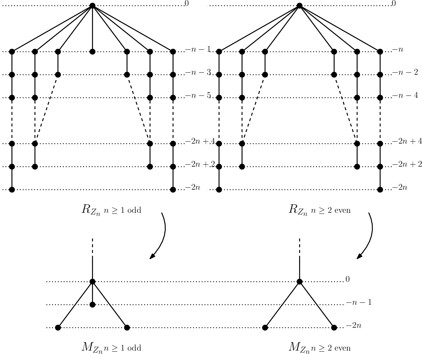
Refer to caption
Figure 7. The minimal graded and monotone subroots of {Zn}n=1∞\{Z_{n}\}^{\infty}_{n=1}.
Remark 4.22.

For the families {Yn}n=1∞\{Y_{n}\}^{\infty}_{n=1} and {Zn}n=1∞\{Z_{n}\}^{\infty}_{n=1}, our computation experiments indicate that the ratio between the number of leaves of minimal graded subroots and whole graded roots goes to zero as n→∞n\to\infty, see Figure 8 and Figure 9.

Finally, we are able to prove our theorems stated in the introduction.

Proof of Theorem 1.2.

The connected Heegaard Floer homology is defined over the minus flavor of Heegaard Floer homology, see Theorem 3.5 or [HHL21, Definition 3.2]. On the homology level, the transition from the plus flavour of Heegaard Floer homology to the negative one can be done by changing the grading with minus version and subtracting two, [OS06, Proposition 7.11]. Using Némethi’s isomorphism in (2.4), this is also true for the lattice homology up to the relevant grading shift.

We compute monotone roots of {Yn}n=1∞\{Y_{n}\}^{\infty}_{n=1} and {Zn}n=1∞\{Z_{n}\}^{\infty}_{n=1} in Proposition 4.14 and Proposition 4.21, respectively. In turn they are displayed in Figure 6 and Figure 7. One can apparently see the transition described above by comparing Figure 1 with Figure 6 and Figure 7. Using Theorem 3.5 and Corollary 3.6 of Hendricks, Hom and Lidman, we complete the proof, see Table 1 for the exposition.

∎

Proof of Theorem 1.3.

The monotone subroots of {Yn}n∈ℕ\{Y_{n}\}_{n\in\mathbb{N}} and {Zn}n∈ℕ\{Z_{n}\}_{n\in\mathbb{N}} are shown in Figure 6 and Figure 7, respectively. Then we list the invariants of Θℤ3\Theta^{3}_{\mathbb{Z}} corresponding to our families in Table 2.

dd-invariant n≥1n\geq 1 odd n≥2n\geq 2 even μ¯\bar{\mu}-invariant n≥1n\geq 1 odd n≥2n\geq 2 even
[Yn][Y_{n}] −2​n-2n −2​n-2n [Yn][Y_{n}] 00 −n2-\frac{n}{2}
[Zn][Z_{n}] −2​n-2n −2​n-2n [Zn][Z_{n}] −n−12\frac{-n-1}{2} 00
Table 2. The homology cobordism invariants of {Yn}n∈ℕ\{Y_{n}\}_{n\in\mathbb{N}} and {Zn}n∈ℕ\{Z_{n}\}_{n\in\mathbb{N}}.

Applying Theorem 3.2, now we are able to parametrize monotone subroots of {Yn}n=1∞\{Y_{n}\}^{\infty}_{n=1} and {Zn}n=1∞\{Z_{n}\}^{\infty}_{n=1} under the homomorphism hh of Hendricks, Manolescu and Zemke in (3.1). When nn is odd, we have

h⁡([Yn])=M⁡(2​n,0).h([Y_{n}])=M(2n,0).

For even values of nn, we find

h⁡([Yn])\displaystyle h([Y_{n}]) =M⁡(2​n,0,n,n),\displaystyle=M(2n,0;n,n),
=M⁡(2​n,0)+M⁡(n,n)−M⁡(n,0),\displaystyle=M(2n,0)+M(n,n)-M(n,0),
=(M⁡(2​n,0)−M⁡(n,0))​[−n].\displaystyle=(M(2n,0)-M(n,0))[-n].

Similarly, if nn is odd, then we obtain

h⁡([Zn])\displaystyle h([Z_{n}]) =M⁡(2​n,0,n+1,n+1),\displaystyle=M(2n,0;n+1,n+1),
=M⁡(2​n,0)+M⁡(n+1,n+1)−M⁡(n+1,0),\displaystyle=M(2n,0)+M(n+1,n+1)-M(n+1,0),
=(M⁡(2​n,0)−M⁡(n+1,0))​[−n−1].\displaystyle=(M(2n,0)-M(n+1,0))[-n-1].

When nn is even, we have

h⁡([Zn])=M⁡(2​n,0).h([Z_{n}])=M(2n,0).

Under the forgetful homomorphism from ℑ{\mathfrak{I}} to ℑ^\widehat{\mathfrak{I}}, we find that

h^​([Yn])={𝒞⁡(−,n),n​is odd,𝒞⁡(−,n)−𝒞⁡(−,n/2),n​is even.\widehat{h}([Y_{n}])=\begin{cases}\mathcal{C}(-,n),&n\ \text{is odd},\\ \mathcal{C}(-,n)-\mathcal{C}(-,n/2),&n\ \text{is even}.\end{cases}

and

h^​([Zn])={𝒞⁡(−,n)−𝒞⁡(−,(n+1)/2),n​is odd,𝒞⁡(−,n),n​is even.\widehat{h}([Z_{n}])=\begin{cases}\mathcal{C}(-,n)-\mathcal{C}(-,(n+1)/2),&n\ \text{is odd},\\ \mathcal{C}(-,n),&n\ \text{is even}.\end{cases}

Next we use the family of homomorphisms {ϕk}k∈ℕ\{\phi_{k}\}_{k\in\mathbb{N}} in (3.2) and we get

ϕk​(𝒞​(−,n))\displaystyle\phi_{k}(\mathcal{C}(-,n)) =δn,k,\displaystyle=\delta_{n,k},
ϕk​(𝒞⁡(−,n/2))\displaystyle\phi_{k}(\mathcal{C}(-,n/2)) =δn/2,k,\displaystyle=\delta_{n/2,k},
ϕk​(𝒞⁡(−,(n+1)/2))\displaystyle\phi_{k}(\mathcal{C}(-,(n+1)/2)) =δ(n+1)/2,k.\displaystyle=\delta_{(n+1)/2,k}.

where δ\delta denotes Kronecker delta function. Therefore, the remaining claim follows from Theorem 3.4 of Dai, Hom, Stoffregen and Truong.

Finally we compare homology cobordism classes of our families with the family of Dai, Hom, Stoffregen and Truong.

From the discussion of Floer theoretic invariants, we see that {Xn}n=1∞\{X_{n}\}^{\infty}_{n=1} is not homology cobordant {Yn}n=1∞\{Y_{n}\}^{\infty}_{n=1} for even values of nn. When nn is odd, {Xn}n=1∞\{X_{n}\}^{\infty}_{n=1} and {Zn}n=1∞\{Z_{n}\}^{\infty}_{n=1} are not homology cobordant as well. Moreover, {Yn}n=1∞\{Y_{n}\}^{\infty}_{n=1} and {Zn}n=1∞\{Z_{n}\}^{\infty}_{n=1} are not homology cobordant for every nn.

Note that the ASL graph has the central vertex −2-2, see Figure 3. Due to the short-cut of Neumann and Zagier [NZ85], RR-invariant of Fintushel and Stern [FS85] of these families can be directly computed as follows:

R⁡([Xn])=R⁡([Yn])=R⁡([Zn])=1for all​n∈ℕ.R([X_{n}])=R([Y_{n}])=R([Z_{n}])=1\ \ \ \text{for all}\ n\in\mathbb{N}.

One can easily verify that for any n∈ℕn\in\mathbb{N} with n>1n>1 we have

(2​n+1)​(4​n+1)​(4​n+3)<(2​n+1)​(3​n+2)​(6​n+1),(2n+1)(4n+1)(4n+3)<(2n+1)(3n+2)(6n+1),

and for all n∈ℕn\in\mathbb{N}

(2​n+1)​(4​n+1)​(4​n+3)<(2​n+1)​(3​n+1)​(6​n+5).(2n+1)(4n+1)(4n+3)<(2n+1)(3n+1)(6n+5).

By [Fur90, Corollary 2.1], we conclude that the family of Dai, Hom, Stoffregen and Truong is not homology cobordant to our two families with an exception X1=Σ⁡(3,5,7)=Y1X_{1}=\Sigma(3,5,7)=Y_{1}. This obstruction also can be successfully done by new gauge theoretic invariants of Daemi [Dae20] and Nozaki, Sato and Taniguchi [NST19]. ∎

Refer to caption
Figure 8. The whole graded roots of Y1,Y2Y_{1},Y_{2} and Y3Y_{3} with minimal graded subroots drawn in dark black.
Refer to caption
Figure 9. The whole graded roots of Z1,Z2Z_{1},Z_{2} and Z3Z_{3} with minimal graded subroots drawn in dark black.

References

  • [AKS20] Antonio Alfieri, Sungkyung Kang, and András I. Stipsicz, Connected Floer homology of covering involutions, Math. Ann. 377 (2020), no. 3-4, 1427–1452. MR 4126897
  • [CK14] Mahir B. Can and Çağrı Karakurt, Calculating Heegaard-Floer homology by counting lattice points in tetrahedra, Acta Math. Hungar. 144 (2014), no. 1, 43–75. MR 3267169
  • [CL85] Thomas D. Cochran and W.B. Raymond Lickorish, Unknotting information from 44-manifolds, Trans. Amer. Math. Soc. 297 (1985), no. 1, 125–142. MR 0849471
  • [Dae20] Aliakbar Daemi, Chern-Simons functional and the homology cobordism group, Duke Math. J. 169 (2020), no. 15, 2827–2886. MR 4158669
  • [Dai18] Irving Dai, On the Pin⁡(2)\mathrm{Pin(2)}-equivariant monopole Floer homology of plumbed 3-manifolds, Michigan Math. J. 67 (2018), no. 2, 423–447. MR 3802260
  • [DHST18] Irving Dai, Jennifer Hom, Matthew Stoffregen, and Linh Truong, An infinite-rank summand of the homology cobordism group, Preprint (2018), arXiv:1810.06145.
  • [DHST21] by same author, More concordance homomorphisms from knot Floer homology, Geom. Topol. 25 (2021), no. 1, 275–338. MR 4226231
  • [DM19a] Irving Dai and Ciprian Manolescu, Involutive Heegaard Floer homology and plumbed three-manifolds, J. Inst. Math. Jussieu 18 (2019), no. 6, 1115–1155. MR 4021102
  • [DM19b] Irving Dai and Maggie Miller, The 00-concordance monoid is infinitely generated, Preprint (2019), arXiv:1907.07166, , To appear in Proc. Amer. Math. Soc.
  • [DS19] Irving Dai and Matthew Stoffregen, On homology cobordism and local equivalence between plumbed manifolds, Geom. Topol. 23 (2019), no. 2, 865––924. MR 3939054
  • [EN85] David Eisenbud and Walter D. Neumann, Three-dimensional link theory and invariants of plane curve singularities, Annals of Mathematics Studies, vol. 110, Princeton University Press, Princeton, NJ, 1985. MR 0817982
  • [End95] Hisaaki Endo, Linear independence of topologically slice knots in the smooth condorcance group, Topology Appl. 63 (1995), no. 3, 257–262. MR 1659565
  • [Fre82] Micheal H. Freedman, The topology of four-dimensional manifolds, J. Differential Geom. 17 (1982), 357–453. MR 0679066
  • [Frø02] Kim A. Frøyshov, Pin(2)-equivariant Seiberg-Witten Floer homology and the triangulation conjecture, Topology 41 (2002), no. 3, 525–552. MR 1910040
  • [FS85] Ronald Fintushel and Ronald J. Stern, Pseudofree orbifolds, Ann. of Math.(2) 122 (1985), no. 2, 335–364. MR 0808222
  • [FS90] by same author, Instanton homology of Seifert fibred homology three spheres, Proc. London Math. Soc.(3) 61 (1990), no. 1, 109–137. MR 1051101
  • [Fur90] Mikio Furuta, Homology cobordism group of homology 33-spheres, Invent. Math. 100 (1990), no. 2, 339–355. MR 1047138
  • [HHL21] Kristen Hendricks, Jennifer Hom, and Tye Lidman, Applications of involutive Heegaard Floer homology, J. Inst. Math. Jussieu 20 (2021), no. 1, 187–224. MR 4205781
  • [HKL16] Jennifer Hom, Çağrı Karakurt, and Tye Lidman, Surgery obstructions and Heegaard Floer homology, Geom. Topol. 20 (2016), no. 4, 2219–2251. MR 3548466
  • [HM17] Kristen Hendricks and Ciprian Manolescu, Involutive Heegaard Floer homology, Duke Math. J. 166 (2017), no. 7, 1211–1299. MR 3649355
  • [HMZ18] Kristen Hendricks, Ciprian Manolescu, and Ian Zemke, A connected sum formula for involutive Heegaard Floer homology, Selecta Math. (N.S.) 24 (2018), 1183–1245. MR 3782421
  • [Ker65] Michel A. Kervaire, On higher dimensional knots, Differential and Combinatorial Topology (A Symposium in Honor of Marston Morse), Princeton Univ. Press, Princeton, N.J., 1965, pp. 105–119. MR 0178475
  • [KO18] Çağrı Karakurt and Ferit Öztürk, Contact structures on AR-singularity links, Internat. J. Math. 29 (2018), no. 3, 185–224. MR 3786529
  • [KŞ20] Çağrı Karakurt and Oğuz Şavk, Ozsváth-Szabó dd-invariants of almost simple linear graphs, J. Knot Theory Ramifications 29 (2020), no. 5, 2050029, 17. MR 4118004
  • [Man18] Ciprian Manolescu, Homology cobordism and triangulations, Proceedings of the International Congress of Mathematicians—Rio de Janeiro 2018. Vol. II. Invited lectures, World Sci. Publ., Hackensack, NJ, 2018, pp. 1175–1191. MR 3966804
  • [Mel77] Paul Michael Melvin, Blowing up and down in 4-manifolds, ProQuest LLC, Ann Arbor, MI, 1977, Thesis (Ph.D.)–University of California, Berkeley. MR 2627246
  • [Ném05] András Némethi, On the Ozsváth-Szabó invariant of negative definite plumbed 3-manifolds, Geom. Topol. 9 (2005), 125–144. MR 2140997
  • [Neu80] Walter D. Neumann, An invariant of plumbed homology spheres, Proc. Sympos., Univ. Siegen, Siegen, 1979, Lecture Notes in Math., vol. 788, Springer, Berlin, 1980, pp. 125–144. MR 0585657
  • [NN05] András Némethi and Liviu I. Nicolaescu, Seiberg-Witten invariants and surface singularities: splicings and cyclic covers, Selecta Math. (N.S.) 11 (2005), no. 3-4, 399–451. MR 2215260
  • [NST19] Yuta Nozaki, Kouki Sato, and Masaki Taniguchi, Filtered instanton Floer homology and the homology cobordism group, Preprint (2019), arXiv:1905.04001, To appear in J. Eur. Math. Soc.
  • [NZ85] Walter D. Neumann and Don Zagier, A note on an invariant of Fintushel and Stern, Geometry and topology (College Park, Md., 1983/84), Lecture Notes in Math., vol. 1167, Springer, Berlin, 1985, pp. 241–244. MR 827273
  • [OS03a] Peter Ozsváth and Zoltán Szabó, Absolutely graded Floer homologies and intersection form for four-manifolds with boundary, Adv. Math. 173 (2003), no. 2, 179–261. MR 1957829
  • [OS03b] by same author, On the Floer homology of plumbed three-manifolds, Geom. Topol. 7 (2003), 185–224. MR 1988284
  • [OS06] Peter Ozsváth and Zoltán Szabó, Holomorphic triangles and invariants for smooth four-manifolds, Adv. Math. 202 (2006), no. 2, 326–400. MR 2222356
  • [OSS17] Peter Ozsváth, András Stipsicz, and Zoltán Szabó, Concordance homomorphisms from knot Floer homology, Adv. Math. 315 (2017), 366–426. MR 3667589
  • [Sav02] Nikolai Saveliev, Invariants for homology 33-spheres, Encyclopedia of Mathematical Sciences, Low-dimensional topology, vol. 140, Springer-Verlag, Berlin, Germany, 2002. MR 1941324
  • [Şav20] Oğuz Şavk, Classical and new plumbed homology spheres bounding contractible manifolds, Preprint (2020), arXiv:2012.12587, To appear in Internat. J. Math.
  • [Sie80] Laurance Siebenmann, On vanishing of the Rohlin invariant and nonfinitely amphicheiral homology 33-spheres, Proc. Sympos., Univ. Siegen, Siegen, 1979, Lecture Notes in Math., vol. 788, Springer, Berlin, 1980, pp. 172–222. MR 0585660
  • [Sto17] Matthew Stoffregen, Manolescu invariants of connected sums, Proc. Lond. Math. Soc. (3) 115 (2017), no. 5, 1072–1117. MR 3733559
  • [Sun21] Nathan Sunukjian, 0-concordance of 2-knots, Proc. Amer. Math. Soc. 149 (2021), no. 4, 1747–1755. MR 4242329
  • [SYZ21] Karthik Seetharaman, William Yue, and Isaac Zhu, Patterns in the lattice homology of Seifert homology spheres, Preprint (2021), arXiv:2110.13405.
  • [Zee65] E. C. Zeeman, Twisting spun knots, Trans. Amer. Math. Soc. 115 (1965), 471–495. MR 195085