Analogue viscous current flow near the onset of superconductivity
Abstract
Spatially resolved transport in two-dimensional quantum materials can reveal dynamics which is invisible in conventional bulk transport measurements. We predict striking patterns in spatially inhomogeneous transport just above the critical temperature in two-dimensional superconducting thin films, where electrical current will appear to flow as if it were a viscous fluid obeying the Navier-Stokes equations. Compared to viscous electron fluids in ultrapure metals such as graphene, this analogue viscous vortex fluid can exhibit a far more tunable crossover, as a function of temperature, from Ohmic to non-local transport, with the latter arising on increasingly large length scales close to the critical temperature. Experiments using nitrogen vacancy center magnetometry, or transport through patterned thin films, could reveal this analogue viscous flow in a wide variety of materials.
1 Introduction
Despite transport being arguably the simplest possible experiment in solid-state physics, the electrical conductivity can also be the most challenging quantity to predict theoretically, especially in strongly correlated systems. Over the coming decade, it will be increasingly possible to measure not only the bulk conductivity , but also a wave number dependent conductivity , using either microscopically-etched devices McGuinness et al. 2021, flows through channels of variable width de Jong and Molenkamp 1995; Moll et al. 2016; Gooth et al. 2018, or local imaging probes. For example, nitrogen vacancy centers in diamond can be high-sensitive, nanometer-resolution magnetometers used to image electric current flow Ku et al. 2020; Jenkins et al.; Vool et al. 2020. Scanning electron tunneling Sulpizio et al. 2019; Krebs et al. 2021; Kumar et al. 2021 could also be used to map local electric potential on similarly short distance scales. Clear predictions for what these future experiments will image across the plethora of discovered phases of quantum matter is a timely endeavor Qi and Lucas 2021; Huang and Lucas 2021.
Here, we study theoretically the spatially-resolved transport of a two-dimensional metallic system near the onset of superconductivity in the absence of external magnetic fields. We consider a system at temperature just above the critical temperature , below which there is superconductivity and essentially no bulk resistivity. The experimental signature which gives superconductivity its name is that the bulk conductivity as from above. Yet is not likely to diverge as well: at finite , the system will already appear ordered – nothing should seem singular at . On phenomenological grounds, we can therefore conclude that
| (1) |
where and are approximately -independent constants. Space-resolved transport should be quite dramatic if stays finite at fixed as .
We will argue that (1) indeed holds, with exponent . This dependence on is mathematically equivalent to what happens in a viscous electron fluid Lucas and Fong 2018; Crossno et al. 2016; Bandurin et al. 2016; Guo et al. 2017; Kumar et al. 2017; Ku et al. 2020. Our theoretical results are grounded in the well-established physics of vortex dynamics near the BKT crossover in two-dimensional superconducting thin films Kosterlitz and Thouless 1973; Halperin and Nelson 1979; Ambegaokar et al. 1980; Petschek and Zippelius 1981; Minnhagen 1987, developed 40 years ago. The main result of this work is predicting the direct experimental signature of vorticity diffusion in non-local conductivities, which can in turn lead to analogue viscous current flows detectable in experiments. Our theoretical perspective follows closely more recent work Davison et al. 2016; Delacrétaz and Hartnoll 2018, and is suited for the strongly correlated dynamics at . The length scale below which the response will appear viscous is set by the typical inter-vortex spacing, which diverges as . In a sufficiently clean device, it may be possible to image “viscous” flow patterns on large length scales just above . Superconducting thin films are thus predicted to be an excellent platform to realize viscous current flow patterns, more robustly than in normal metals such as graphene or GaAs. Analyzing this analogue viscous flow can reveal fundamental information about the dynamics of strongly correlated electrons which is otherwise invisible in bulk resistance measurements.
2 Spatially resolved transport
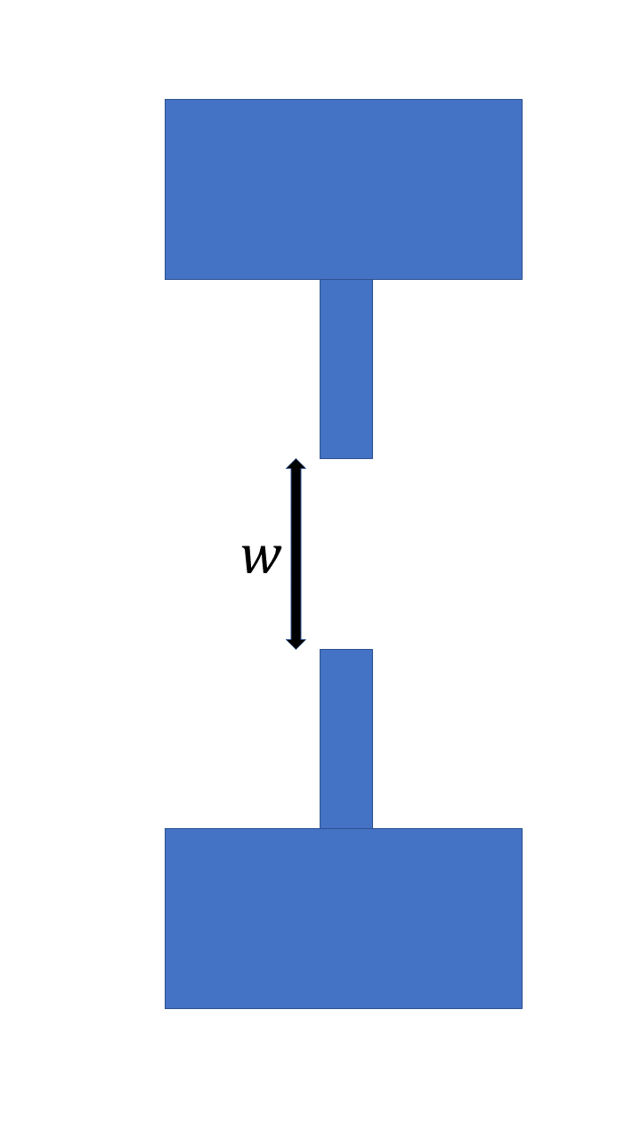
Before describing our derivation of (1), let us explain how this quantity can be (indirectly) probed in experiment. Due to the large speed of light , one cannot simply shine light on a sample, since is very large (in fact, it is then more appropriate to approximate while ).
We advocate the following strategy instead. Consider etching a constriction into a 2d material, as sketched in Figure 1. The blue region dictates the region where current cannot traverse. In experiments on graphene this is done by applying a bias voltage over the constriction, forming an effectively “hard wall” region where the Fermi energy is very different. When applying a constant uniform transverse electric field, the presence of these “hard walls” modifies the current flow pattern. A microscopically exact treatment of this problem has never been found. To compare with existing experimental data Jenkins et al., therefore, a more phenomenological approach is needed. Consider the formal equations
| (2a) | ||||
| (2b) | ||||
where and are the background and induced electric fields respectively. The induced electric fields will vanish except inside of the forbidden regions where electrons cannot traverse. We thus require that outside the walls , while inside . Making a final assumption that (the sample is otherwise approximately homogeneous), one can look for solutions to (2) consistent with these requirements. This prescription has been detailed at some length elsewhere Huang and Lucas 2021; Qi and Lucas 2021. The key thing which has been found is that the current flow pattern is qualitatively modified by , which is simply the Fourier transform of :
| (3) |
Assuming translation invariance, the spatially dependent conductivity can be formally defined as
| (4) |
3 Analogue viscous flow in superconducting thin films
Consider a two-dimensional metal (or a thin film of thickness of an intrinsically three-dimensional metal) at temperature just above a superconducting transition temperature (here corresponds to ). In the 3d case, we require , where is the 3d coherence length of the superconductor, which will be finite at the critical temperature of the 2d film. We take , but . In this temperature range, vortices proliferate and destroy (quasi-)long-range order. As , the diverging conductivity is a consequence of the vanishing of “free” vortices (not bound in a vortex-antivortex pair) Bardeen and Stephen 1965.
We acknowledge that the Aslamazov-Larkin (AL) theory of fluctuations Galitski 2008; Galitski and Larkin 2001; Aslamazov and Larkin 1968, which strictly holds above , can describe many experimental situations quite close to (which is in turn very close to ). While we point out that the AL theory does not hold for , there may be a narrow temperature window where the effects we predict are visible, and those of the AL theory are not. We leave a precise answer to this question to future work.
Strictly speaking, an essential difference between a superconductor and superfluid becomes important close to : as the supercurrents that circulate around a vortex generate a magnetic field, this leads to an effective potential energy between vortices that scales as instead of the usual interaction of the superfluid Pearl 1964. However, in typical superconductors, the crossover between these power laws occurs at distances mm Halperin and Nelson 1979; Beasley et al. 1979. As this length scale is orders of magnitude larger than the mesoscopic samples we advocate looking for analogue viscosity in, we can safely neglect this correction. Henceforth, we can approximate that vortex dynamics will be the same as in a neutral superfluid.
To understand the implications of these long-lived vortices in transport, we observe that for , there is a long-lived supercurrent . In general, computing is incredibly challenging. However, because is long-lived, we expect to be dominated by the relaxation of Davison et al. 2016; Delacrétaz and Hartnoll 2018.
To explain more quantitatively, let be the superfluid velocity, which is thermodynamically conjugate to . On general grounds Davison et al. 2016; Forster 1995; Lucas and Sachdev 2015,
| (5) |
Using the memory matrix formalism Hartnoll et al. 2018; Lucas and Sachdev 2015, one can show that
| (6) |
Here is the relaxation rate of the supercurrent:
| (7) |
Precise computations of any of the three terms in (6) are difficult near in any microscopic model, but we can reliably estimate the scaling of each term, beginning with the susceptibilities. Importantly, we find that and are finite as , and do not exhibit power law dependence in . In the absence of rotational symmetry breaking, one can define them as follows: Davison et al. 2016; Delacrétaz and Hartnoll 2018
| (8) |
Here the superfluid boson degree of freedom has mass and charge , and is the local bare superfluid density outside of vortex cores, which is finite near Halperin and Nelson 1979: see the appendices for further discussions. For simplicity writing , we conclude that
| (9) |
The non-trivial calculation is thus of .
is where the vortex physics highlighted earlier becomes important. The superfluid velocity is the gradient of a phase, a U(1) order parameter which exhibits point-like defects called vortices in two dimensions. The stable vortices have phase which winds by around a point: let us denote the density of free positive circulation and negative circulation vortices with and respectively. The density of free vortices is given by , where Ambegaokar et al. 1980; Minnhagen 1987
| (10) |
with a material-dependent constant (usually Mondal et al. 2011). In contrast, the signed vortex density is
| (11) |
Since spatial variations are aligned along ,
| (12) |
and thus we can deduce the leading order behavior in by calculating the signed vortex decay rate.
Just above the vortices form an analogue “Coulomb gas” Minnhagen 1987 of free charges (vortices); the superfluid velocity is orthogonal to an effective electric field that would be generated by the charges. can thus be deduced via the relaxation of externally imposed charges in a two-dimensional plasma. If there were no free vortices (, or ), then we expect diffusive relaxation: on length scales , simply because this is the generic hydrodynamics of a conserved quantity Ambegaokar et al. 1980; Petschek and Zippelius 1981. However, due to long-range interactions between vortices, is finite if : the mechanism is mathematically identical to the finite time decay of free charges in Maxwell’s equations with an Ohmic current (). Hence for a constant (see SM for details),
| (13) |
indicates higher-order terms suppressed by additional powers of . Combining (6), (8) and (13), we find
| (14) |
This is the main result of our paper. Our claim is that (14) captures the generic scaling of both when , and when , independently of the microscopic details. This is because in a generic superfluid, the only parametrically long-lived mode near is the supercurrent. If we take in (14), we have just computed the bulk conductivity of the metal just above . The divergence in conductivity as one approaches superconductivity follows from the vanishing of free vortex density, which is simply the Bardeen-Schrieffer “flux flow conductivity” Bardeen and Stephen 1965, which has been experimentally observed Abraham et al. 1982; Resnick et al. 1981; Kadin et al. 1983. In the limit of finite , (14) implies . This can intuitively be thought of as a consequence of vortex diffusion. In the SM, we discuss why there are indeed no anomalous corrections to diffusion (a point first made in Petschek and Zippelius 1981), and that the diffusion constant itself (while being the physical diffusion constant for vorticity relaxation) is dominated by the response of tightly bound vortex pairs. Importantly, (14) applies to both conventional and unconventional superconductors, as the arguments for the form of make no reference to the conventional BCS theory of superconductivity.
Remarkably, the exact same mathematical structure as (14) also arises if one models the electrons as a viscous fluid Lucas and Fong 2018; Crossno et al. 2016; Bandurin et al. 2016; Guo et al. 2017; Kumar et al. 2017: solving the Navier-Stokes equations in the presence of impurities, one finds Huang and Lucas 2021; Qi and Lucas 2021
| (15) |
where is the normal charge density and is the shear viscosity, and the scattering rate off of impurities, which relaxes momentum, is proportional to . The mathematical analogy between (14) and (15) makes precise our claim that one can look for analogue viscous flows just above . We emphasize however that in general, a viscous electron fluid only arises when there is approximate momentum conservation in electronic collisions, which is a very rare criterion (most metals are quity dirty). In contrast, any metal with a superconducting transition will eventually reach a regime very close to where . So it should be easier to see “viscous flows” near the onset of superconductivity, than in a genuinely viscous electron fluid.
As we detail in Appendix B, our microscopic argument for the scaling assumes that we are exactly at ; it is possible that for , corrections to this scaling arise. While our microscopic argument does not suggest that the exponents of the equilibrium inter-vortex distribution modify the scaling exponent in , a more detailed analysis could be worthwhile. Even if such corrections do eventually emerge far from the critical temperature, from an experimental point of view, observing these corrections could be challenging, as even observing the scaling given in (14) will require a carefully designed experiment!
4 Comparison to previous studies
There have been several older studies looking at viscosity in the context of vortex liquids in superconductors and we now compare our findings to earlier work. The first studies of Marchetti and Nelson 1991; Radzihovsky and Frey 1993; Huse and Majumdar 1993; Mou et al. 1995; Wortis and Huse 1996; Marchetti and Nelson 1990 focused on the dynamics of melted Abrikosov flux lattices in large magnetic fields, whereas our work focuses on the zero field limit. Moreover, what we call “analogue viscosity” is not the same as the vortex viscosity identified in these references, which was taken to be the -coefficient of a Taylor expansion of . Therefore, they claimed that . Comparing (14) and (15) we see that . Finally, Wortis and Huse 1996 argues that in this regime, is a non-monotonic function which increases at small , not at all like (14). Interestingly nevertheless, was found in Mou et al. 1995 in the limit , although this calculation could not explain the origin of near from vortex physics, which is a non-perturbatively small correction at high . In our calculation we implicitly assumed a strongly interacting vortex liquid near .
The physics responsible for analogue viscosity was first identified in an even older literature Ambegaokar et al. 1980; Petschek and Zippelius 1981 on vortex diffusion in superfluid thin films. The contribution of this work is (14): vorticity diffusion should be readily measurable via non-local conductivity . In other settings, authors have found logarithmic corrections to Huber 1982; Ginzburg et al. 1997 which arise due to long-range interactions between vortices. However, as argued in Petschek and Zippelius 1981, we do not expect this effect to arise near the onset of superconductivity: see Appendix. In any case, the existence or not of any logarithmic corrections in will be quite hard to detect in experiment.
It has also been recently argued Liao and Galitski 2019 that the true shear viscosity is strongly -dependent close to . However, we emphasize that our mechanism is qualitatively distinct: the perturbative calculation of Liao and Galitski 2019 which suggests viscous flow in superconducting metals is in the regime , whereas our calculation holds when .
5 Experimental implications
The link between vortex diffusion and non-local conductivity identified in this work has serious experimental implications, as we now discuss. Due to the large speed of light, optical probes readily measure , rather than ; indeed, 40 years ago, most experimental works focused on finite (not ) response for this reason. However, we have emphasized here that is a direct window into vortex diffusion, an effect which is readily seen in . Perhaps the most direct way to measure the latter is by using local magnetometry. One can either measure current fluctuations (which give due to the fluctuation-dissipation theorem Agarwal et al. 2017), or simply image current flow patterns Ku et al. 2020; Jenkins et al.; Vool et al. 2020 and deduce the resulting Huang and Lucas 2021; Qi and Lucas 2021. Imaging techniques such as nitrogen-vacancy center magnetometry have been successfully demonstrated at 6 K Pelliccione et al. 2015, meaning that this technique is capable of testing our predictions in conventional superconducting thin films. This imaging can be done at nm, but even assuming that we can only probe much larger length scales m, we could detect a crossover from Ohmic to viscous flow patterns when . After all, the free vortex spacing diverges near . Using estimates and nm from NbN thin films Mondal et al. 2011; Yong et al. 2013 (which we expect are reasonable order-of-magnitude estimates for most conventional superconducting thin films), one must be within about 0.1% of 7.7 K in order to find m. At this length scale the resistivity will be reduced by the factor of , which has been resolved in experiment. Hence we expect such precision in is achievable, albeit may prove challenging in magnetometry experiments (where a rise in temperature due to electronic heating must be balanced against the current density which is detectable by the magnetometer itself.
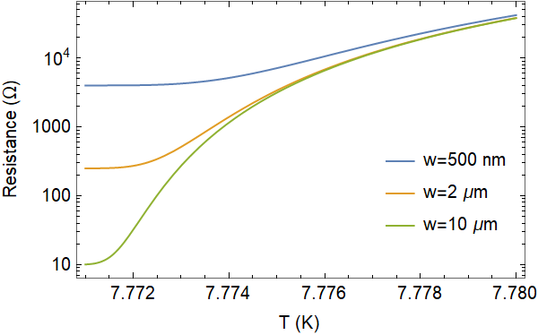
If probing directly is not possible, one may alternatively engineer devices with narrow constrictions through which current is forced to flow. Mirroring known results for viscous electron fluids Guo et al. 2017; Kumar et al. 2017, we estimate the resistance of the device sketched in Figure 1 as
| (16) |
where will depend on the geometry of the device and may exhibit some dependence on ratios of to the size of the device as a whole Kumar et al. 2017. However, once , the dominant contribution to will come from the term, heralding the analogue viscous flow. In Figure 2 we sketch how should look as a function of close to . This prediction assumes that generic boundary conditions hold on the current, and that the current does not exactly follow the unique curl-free flow pattern (see Appendix). Since almost three decades ago non-local transport was observed on m scales in YBCO Safar et al. 1994 in a T field, we expect that currents must obey boundary conditions conducive to the non-local transport described above, at least in some materials.
Patterning such constrictions into a thin film superconductor can be done via focused ion beam etching Moll et al. 2016. Alternatively, local gates above the device can be used to imprint a constriction geometry, as is readily done in graphene-based devices Jenkins et al.. Assuming generic boundary conditions, imaging current flows through these geometries with magnetometers will lead to qualitatively different flow patterns in Ohmic regimes () vs. non-local regimes (e.g. ), and is a more compelling experimental probe of non-local transport than a conductance measurement by itself.
6 Discussion and conclusion
A natural candidate material to test our theory is MoGe Mason and Kapitulnik 1999, which exhibits an “anomalous” metal which is likely a failed superconductor Davison et al. 2016. A rather different application of this technique could be to gain further insight into the “strange metal” phase observed in both twisted magic-angle bilayer graphene Polshyn et al. 2019; Cao et al. 2020; Jaoui et al. 2022, and thin films of a cuprate superconductor Wu et al. 2017. Understanding the role played by vortices and phase fluctuations in bad metals could help deduce the origin -linear resistivity and provide a further check for universality in dynamics from one material to the next. Evidence for such a conjecture thus far relies on the universality of “Planckian” scattering rates in bulk transport; imaging local currents will provide an important check into the interplay of non-quasiparticle physics with the onset of ordering. In particular, Planckian-limited scattering rates might be observed in the diffusion constant , even as the bulk resistivity (which is approaching zero near , and is clearly well below the Planckian bound conjectured in Hartnoll 2015. Therefore, studying spatially resolved transport could reveal valuable insight about potential universal properties of strange metals near . It is predicted Bardeen and Stephen 1965; Davison et al. 2016 that near , the vortex diffusion constant , the electrical resistivity of the normal fluid component. Hence measuring the strength of “analogue viscous flow”, which directly determines , can lead to a test of whether the Planckian scattering responsible for well above , continues to hold at . Additionally, in ordinary superconducting thin films it is expected that Ambegaokar et al. 1980, and it would be interesting to learn experimentally whether the alternative bound proposed in Hartnoll 2015 holds near the superconducting transition of a strange metal.
One challenge for realizing this non-local transport over parametrically large scales in a real material may be inhomogeneities – not because they can directly relax the “viscous” mode as in a conventional electron fluid Lucas and Fong 2018, but because they could cause to substantially vary throughout the device Spivak et al. 2008. This inhomogeneity could put a fundamental limit on the regime of validity of our theory, which may not capture dynamics across superconducting islands. Testing our predictions in materials where the onset of superconductivity appears quite sharp, as measured in device resistance as a function of temperature, may be a practical way to minimize these effects Beasley et al. 1979. On the other hand, dirty superconductors have a broader crossover in the resistivity , suggesting that less temperature control will be necessary to access regimes close to where vortex physics can dominate. Future experiments will help to deduce the criteria and materials where non-local transport is most readily observed in a superconducting thin film.
Acknowledgements
We thank Luca Delacretaz, Dan Dessau, Sean Hartnoll, and especially David Huse and Leo Radzihovsky, for helpful discussions. This work was supported by the Alfred P. Sloan Foundation through Grant FG-2020-13795 (AL), and by the Gordon and Betty Moore Foundation’s EPiQS Initiative via Grant GBMF10279 (KG, AL).
Appendix A Thermodynamics
To motivate (8), consider a microscopic Ginzburg-Landau theory of a superconductor with Lagrangian
| (17) |
Here is the mass of the condensing boson (which for conventional superconductors is the Cooper pair) and its charge. Writing , the supercurrent is
| (18) |
with . Far from a vortex core, we have , the bare superfluid density. Hence we obtain
| (19) |
and we do not expect this susceptibility to exhibit strong -dependence.
Next we turn to . This is a little more subtle because, as emphasized in the main text, is closely related to vortex physics, which can seem singular as . We invoke the Coulomb gas analogy to a charged plasma, where we can calculate the vortex susceptibility using the following identity relating (analogue) charge susceptibility to permittivity Mahan 2010:
| (20) |
where is the bare dielectric constant without including free vortices and the polarization of bound vortices (which we keep just for clarity, though it may as well be 1). One expects that for (for some constant and O(1) constant ) Minnhagen 1987
| (21) |
where is a non-singular term. The first term is extremely singular and corresponds to the Poisson-Boltzmann screening of point charges whenever , since the combined potential ; the second term is regular and just corresponds to microscopic scale corrections to the Coulomb gas analogy to point charges. Combining (20) and (21) and neglecting the -term, we find
| (22) |
Combining (22) with (11) and (12) we deduce that
| (23) |
If , we can essentially treat this susceptibility as a constant; if , then this susceptibility could change by some O(1) factor; however this would modify neither limit of our main result (14).
Appendix B Vortex decay time
Now we estimate with the memory matrix formalism Lucas and Sachdev 2015; Forster 1995. Observe that is (generically) the unique parametrically long-lived pseudoscalar operator (at wave number ) in the system; therefore, we can write
| (24) |
where the memory matrix
| (25) |
where is the operator corresponding to the rate of change of vortex density. We may write
| (26) |
where is the vortex current operator. In a semiclassical limit with large vortices,
| (27) |
where indexes the vortices in the system with orientations .
To proceed farther and evaluate the spectral weight (25) we need to make a few more assumptions. For simplicity let us begin working exactly at . Following the Coulomb gas literature, at this point all vortices are “bound” in pairs; letting denote the superfluid healing length (which is finite, and corresponds to roughly the radius of the vortex core), one finds Petschek and Zippelius 1981 that the probability density that a vortex pair is separated by distance is
| (28) |
Let us further assume the dominant contribution to the spectral weight arises from interactions between two vortices in a vortex pair (possibly screened via other more tightly bound pairs, but this is accounted for by renormalized coefficients Minnhagen 1987); in this case we estimate that
| (29) |
where
| (30) |
with denoting the position of the positive/negative vortex in the pair, obeying ; the average This formula is rather imprecise, as a pair will tend to dynamically change its value of over time, but intuitively our approximation is to understand the contribution of each bound pair on its own to .
In the absence of thermal fluctuations and dissipation (both coming due to interaction with the normal fluid), a bound pair will simply propagate in a straight line, perpendicular to the orientation of the vortex dipole. Orienting the dipole for simplicity by placing the vortex at , we find this bound pair’s contribution to
| (31) |
However, since the isolated pair will move in a straight line forever, it’s contribution to would be due to the integral over ; thus we need to also incorporate dissipative effects. In the presence of dissipation (but not thermal noise), a bound vortex pair will deterministically annihilate in a time Chesler and Lucas 2014. Accounting for this finite lifetime, and assuming that interactions with other pairs might only decrease the scaling of this lifetime (e.g. if a tightly bound and weakly bound positive vortex “swap roles” during a close pass, we expect the direction of the bound pair drift to become a bit randomized) we estimate that
| (32) |
where we have taken the limit since, as we will see immediately, the smallest vortex pairs dominate the spectral weight. Plugging in (32) into (29) we obtain
| (33) |
since the integral over is convergent. (Although the convergence is slow, accounting for corrections would give at best , which is subleading compared to the contribution from .). Hence
| (34) |
with no logarithmic corrections despite the power-law nature of the interactions in the system. Indeed, observe that even if our estimate of was too large, because the integral over in is dominated at small not large , a modified can only change by an O(1) constant, but not lead to any anomalous -scaling in the answer at leading order. Petschek and Zippelius 1981 has also confirmed that perturbative corrections to this argument due to other more tightly bound pairs, which serve primarily to renormalize the effective permittivity of the vortex gas, do not lead to singular-in- corrections to these integrals.
We believe that for , the primary difference will be that the probability density decays faster with than given in (28) Minnhagen 1987. This would most likely suppressing subleading -dependent corrections but otherwise, we do not expect it to alter our primary result.
There is one important subtlety overlooked thus far in the argument, which we must address. Naively, the dominant contribution to arises due to the drift of vortex pairs together (or apart), which could contribute (in the absence of noise)
| (35) |
which seems to dominate the scaling found in (31). Indeed, at time , this “dissipative” part of the vortex current will dominate . However, we claim that when integrating the correlator over all time , as in (30), this contribution will be small (at least for the tightly bound pairs). Indeed, suppose that the superfluid consisted of a single bound pair, which popped in and out of existence (mainly staying tightly bound). Applying a weak “analogue electric field” (supercurrent), by the fluctuation-dissipation theorem, the spectral weight will pick up a contribution proportional to the average contribution of this pair to as , even when averaging over orientations of the vortex dipole. This will vanish: the pair is bound and the electric field is not strong enough to overcome the “activation barrier” to pull the pair apart. Moreover, the actual drift of the vortex dipole in the background velocity field does not on average contribute to , as it flips sign when exchanging the positive/negative vortex (and each configuration is equally likely). Thus cannot pick up any contributions from the vortex current associated with fluctuations in vortex distance, unless the vortex pair is widely separated, where the electric field can unbind it. Yet similar to the previous argument, the contributions to from such weakly bound pairs are suppressed by a power of .
For , we expect that
| (36) |
for O(1) constant . In our argumentation, this happens because the bound dipole distribution will truncate at . Beyond this point, the contribution of unbound vortex motion to in (31) will not come with an extra factor of ; thus we will find an additional contribution, of relative magnitude relative to the bound pair contribution; this leads to (36) and thus to (13).
There is a somewhat curious observation that we can make. We have just argued that is dominated by tightly bound pairs; however, from the equation of motion for , we also conclude that the effective diffusion constant of one isolated vortex (also known to be finite Petschek and Zippelius 1981), must be given by the diffusion constant arising due to the dynamics of tightly bound pairs. Perhaps the microscopic mechanism for this vortex’s diffusion is repeated interactions with annihilating/forming vortex pairs nearby, which could nicely explain why the tightly bound pairs appear to control the “macroscopically observable” diffusion constant of net vorticity.
Let us also briefly connect our somewhat microscopic arguments for to the more recent works Davison et al. 2016. They wrote down a constitutive relation for the vortex current:
| (37) |
where . Together with the constitutive relation for the supercurrent (here )
| (38) |
and the relation , one can immediately solve (38) and find that , which leads to (14). In Davison et al. 2016, they did not compute and focused instead on . From this perspective, our argument for is clearly immediate; however, the subtle point is whether or not the vortex interactions, which are necessarily very long ranged, break the gradient expansion of hydrodynamics. In agreement with other authors, we have argued that this does not happen.
Appendix C Boundary conditions
What we have predicted is that any time transverse current flows near , one will see non-local conductivity due to vortex physics. Somewhat annoyingly, it is possible to find a purely longitudinal flow in any two-dimensional geometry for any fixed boundary conditions on the current. Expressing such a current flow pattern as (we have chosen suggestive notation, whereby represents (the diverging bulk conductivity near ) and represents a characteristic voltage profile which would be consistent with Ohmic flow), the uniqueness of solutions to with Neumann boundary conditions implies that one can find a current flow pattern obeying . It is not clear that on this flow pattern vortex physics must be relevant. However, if current flow patterns deviate at all from this special profile, then viscous effects must contribute to the conductance to some degree. Since experiments Safar et al. 1994 have seen some evidence for non-local transport in vortex liquids in superconducting YBCO, we presume that at least in some materials, the boundary conditions are not consistent with purely longitudinal flow.
References
- McGuinness et al. (2021) Philippa H. McGuinness, Elina Zhakina, Markus König, Maja D. Bachmann, Carsten Putzke, Philip J. W. Moll, Seunghyun Khim, and Andrew P. Mackenzie, “Low-symmetry nonlocal transport in microstructured squares of delafossite metals,” Proceedings of the National Academy of Sciences 118, e2113185118 (2021), https://www.pnas.org/doi/pdf/10.1073/pnas.2113185118 .
- de Jong and Molenkamp (1995) M. J. M. de Jong and L. W. Molenkamp, “Hydrodynamic electron flow in high-mobility wires,” Phys. Rev. B 51, 13389–13402 (1995).
- Moll et al. (2016) P. J. W. Moll, P. Kushwaha, N. Nandi, B. Schmidt, and A. P. Mackenzie, “Evidence for hydrodynamic electron flow in PdCoO2,” Science 351, 1061 (2016).
- Gooth et al. (2018) J. Gooth, F. Menges, N. Kumar, V. Suss, C. Shekhar, Y. Sun, U. Drechsler, R. Zierold, C. Felser, and B. Gotsmann, “Thermal and electrical signatures of a hydrodynamic electron fluid in tungsten diphosphide,” Nature Communications 9, 4093 (2018).
- Ku et al. (2020) Mark J. H. Ku, Tony X. Zhou, Qing Li, Young J. Shin, Jing K. Shi, Claire Burch, Laurel E. Anderson, Andrew T. Pierce, Yonglong Xie, Assaf Hamo, Uri Vool, Huiliang Zhang, Francesco Casola, Takashi Taniguchi, Kenji Watanabe, Michael M. Fogler, Philip Kim, Amir Yacoby, and Ronald L. Walsworth, “Imaging viscous flow of the dirac fluid in graphene,” Nature 583, 537–541 (2020).
- (6) A. Jenkins, S. Baumann, H. Zhou, S. A. Meynell, D. Yang, K. Watanabe, T. Taniguchi, A. Lucas, A. F. Young, and A. C. Bleszynski Jayich, arXiv:2002.05065 [cond-mat.mes-hall] .
- Vool et al. (2020) U. Vool, A. Hamo, G. Varnavides, Y. Wang, T. X. Zhou, N. Kumar, Y. Dovzhenko, Z. Qiu, C. A. C. Garcia, A. T. Pierce, et al., (2020), arXiv:2009.04477 [cond-mat.mes-hall] .
- Sulpizio et al. (2019) J. A. Sulpizio, L. Ella, A. Rozen, J. Birkbeck, D. J. Perello, D. Dutta, M. Ben-Shalom, T. Taniguchi, K. Watanabe, T. Holder, et al., Nature 576, 75–79 (2019).
- Krebs et al. (2021) Zachary J. Krebs, Wyatt A. Behn, Songci Li, Keenan J. Smith, Kenji Watanabe, Takashi Taniguchi, Alex Levchenko, and Victor W. Brar, “Imaging the breaking of electrostatic dams in graphene for ballistic and viscous fluids,” (2021), arXiv:2106.07212 [cond-mat.mes-hall] .
- Kumar et al. (2021) Chandan Kumar, John Birkbeck, Joseph A. Sulpizio, David J. Perello, Takashi Taniguchi, Kenji Watanabe, Oren Reuven, Thomas Scaffidi, Ady Stern, Andre K. Geim, and Shahal Ilani, “Imaging hydrodynamic electrons flowing without landauer-sharvin resistance,” (2021), arXiv:2111.06412 [cond-mat.mes-hall] .
- Qi and Lucas (2021) Marvin Qi and Andrew Lucas, “Distinguishing viscous, ballistic, and diffusive current flows in anisotropic metals,” Phys. Rev. B 104, 195106 (2021).
- Huang and Lucas (2021) Xiaoyang Huang and Andrew Lucas, “Fingerprints of quantum criticality in locally resolved transport,” (2021), arXiv:2105.01075 [cond-mat.str-el] .
- Lucas and Fong (2018) A. Lucas and K. C. Fong, “Hydrodynamics of electrons in graphene,” Journal of Physics: Condensed Matter 30, 053001 (2018).
- Crossno et al. (2016) J. Crossno, J. K. Shi, K. Wang, X. Liu, A. Harzheim, A. Lucas, S. Sachdev, P. Kim, T. Taniguchi, K. Watanabe, and et al., “Observation of the Dirac fluid and the breakdown of the Wiedemann-Franz law in graphene,” Science 351, 1058 (2016).
- Bandurin et al. (2016) D. A. Bandurin, I. Torre, R. Krishna Kumar, M. Ben Shalom, A. Tomadin, A. Principi, G. H. Auton, E. Khestanova, K. S. Novoselov, I. V. Grigorieva, L. A. Ponomarenko, A. K. Geim, and M. Polini, “Negative local resistance caused by viscous electron backflow in graphene,” Science 351, 1055 (2016).
- Guo et al. (2017) H. Guo, E. Ilseven, G. Falkovich, and L. S. Levitov, “Higher-than-ballistic conduction of viscous electron flows,” Proceedings of the National Academy of Sciences 114, 3068–3073 (2017).
- Kumar et al. (2017) R. Krishna Kumar, D. A. Bandurin, F. M. D. Pellegrino, Y. Cao, A. Principi, H. Guo, G. H. Auton, M. Ben Shalom, L. A. Ponomarenko, G. Falkovich, and et al., “Superballistic flow of viscous electron fluid through graphene constrictions,” Nature Physics 13, 1182 (2017).
- Kosterlitz and Thouless (1973) J M Kosterlitz and D J Thouless, “Ordering, metastability and phase transitions in two-dimensional systems,” Journal of Physics C: Solid State Physics 6, 1181–1203 (1973).
- Halperin and Nelson (1979) B. I. Halperin and D. R. Nelson, “Resistive transition in superconducting films,” J. Low Temp. Phys. 36, 599 (1979).
- Ambegaokar et al. (1980) Vinay Ambegaokar, B. I. Halperin, David R. Nelson, and Eric D. Siggia, “Dynamics of superfluid films,” Phys. Rev. B 21, 1806–1826 (1980).
- Petschek and Zippelius (1981) R. G. Petschek and Annette Zippelius, “Renormalization of the vortex diffusion constant in superfluid films,” Phys. Rev. B 23, 3483–3493 (1981).
- Minnhagen (1987) Petter Minnhagen, “The two-dimensional coulomb gas, vortex unbinding, and superfluid-superconducting films,” Rev. Mod. Phys. 59, 1001–1066 (1987).
- Davison et al. (2016) Richard A. Davison, Luca V. Delacrétaz, Blaise Goutéraux, and Sean A. Hartnoll, “Hydrodynamic theory of quantum fluctuating superconductivity,” Phys. Rev. B 94, 054502 (2016).
- Delacrétaz and Hartnoll (2018) Luca V. Delacrétaz and Sean A. Hartnoll, “Theory of the supercyclotron resonance and hall response in anomalous two-dimensional metals,” Phys. Rev. B 97, 220506 (2018).
- Bardeen and Stephen (1965) John Bardeen and M. J. Stephen, “Theory of the motion of vortices in superconductors,” Phys. Rev. 140, A1197–A1207 (1965).
- Galitski (2008) Victor Galitski, “Nonperturbative microscopic theory of superconducting fluctuations near a quantum critical point,” Phys. Rev. Lett. 100, 127001 (2008).
- Galitski and Larkin (2001) V. M. Galitski and A. I. Larkin, “Superconducting fluctuations at low temperature,” Phys. Rev. B 63, 174506 (2001).
- Aslamazov and Larkin (1968) L G Aslamazov and A I Larkin, “Effect of fluctuations on the properties of a superconductor above the critical temperature,” Sov. Phys. - Solid State (Engl. Transl.) 10, 875 (1968).
- Pearl (1964) J Pearl, “Current distribution in superconducting films carrying quantized fluxoids,” Applied Physics Letters 5, 65–66 (1964).
- Beasley et al. (1979) M. R. Beasley, J. E. Mooij, and T. P. Orlando, “Possibility of vortex-antivortex pair dissociation in two-dimensional superconductors,” Phys. Rev. Lett. 42, 1165–1168 (1979).
- Forster (1995) D. Forster, Hydrodynamic Fluctuations, Broken Symmetry, And Correlation Functions, Advanced Books Classics (Avalon Publishing, 1995).
- Lucas and Sachdev (2015) Andrew Lucas and Subir Sachdev, “Memory matrix theory of magnetotransport in strange metals,” Phys. Rev. B 91, 195122 (2015).
- Hartnoll et al. (2018) Sean A. Hartnoll, Andrew Lucas, and Subir Sachdev, “Holographic quantum matter,” (2018), arXiv:1612.07324 [hep-th] .
- Mondal et al. (2011) Mintu Mondal, Sanjeev Kumar, Madhavi Chand, Anand Kamlapure, Garima Saraswat, G. Seibold, L. Benfatto, and Pratap Raychaudhuri, “Role of the vortex-core energy on the berezinskii-kosterlitz-thouless transition in thin films of nbn,” Phys. Rev. Lett. 107, 217003 (2011).
- Abraham et al. (1982) David W. Abraham, C. J. Lobb, M. Tinkham, and T. M. Klapwijk, “Resistive transition in two-dimensional arrays of superconducting weak links,” Phys. Rev. B 26, 5268–5271 (1982).
- Resnick et al. (1981) D. J. Resnick, J. C. Garland, J. T. Boyd, S. Shoemaker, and R. S. Newrock, “Kosterlitz-thouless transition in proximity-coupled superconducting arrays,” Phys. Rev. Lett. 47, 1542–1545 (1981).
- Kadin et al. (1983) A. M. Kadin, K. Epstein, and A. M. Goldman, “Renormalization and the kosterlitz-thouless transition in a two-dimensional superconductor,” Phys. Rev. B 27, 6691–6702 (1983).
- Marchetti and Nelson (1991) M. C. Marchetti and D. R. Nelson, “Dynamics of flux-line liquids in high- superconductors,” Physica C 174, 40–62 (1991).
- Radzihovsky and Frey (1993) Leo Radzihovsky and Erwin Frey, “Kinetic theory of flux-line hydrodynamics: Liquid phase with disorder,” Phys. Rev. B 48, 10357–10381 (1993).
- Huse and Majumdar (1993) David A. Huse and Satya N. Majumdar, “Nonlocal resistivity in the vortex liquid regime of type-ii superconductors,” Phys. Rev. Lett. 71, 2473–2476 (1993).
- Mou et al. (1995) Chung-Yu Mou, Rachel Wortis, Alan T. Dorsey, and David A. Huse, “Nonlocal conductivity in type-ii superconductors,” Phys. Rev. B 51, 6575–6587 (1995).
- Wortis and Huse (1996) Rachel Wortis and David A. Huse, “Nonlocal conductivity in the vortex-liquid regime of a two-dimensional superconductor,” Phys. Rev. B 54, 12413–12420 (1996).
- Marchetti and Nelson (1990) M. Cristina Marchetti and David R. Nelson, “Hydrodynamics of flux liquids,” Phys. Rev. B 42, 9938–9943 (1990).
- Huber (1982) D. L. Huber, “Dynamics of spin vortices in two-dimensional planar magnets,” Phys. Rev. B 26, 3758–3765 (1982).
- Ginzburg et al. (1997) Valeriy V. Ginzburg, Leo Radzihovsky, and Noel A. Clark, “Self-consistent model of an annihilation-diffusion reaction with long-range interactions,” Phys. Rev. E 55, 395–402 (1997).
- Liao and Galitski (2019) Yunxiang Liao and Victor Galitski, “Critical viscosity of a fluctuating superconductor,” Phys. Rev. B 100, 060501 (2019).
- Agarwal et al. (2017) K. Agarwal, R. Schmidt, B. Halperin, V. Oganesyan, G. Zaránd, M. D. Lukin, and E. Demler, Phys. Rev. B 95, 155107 (2017).
- Pelliccione et al. (2015) Matthew Pelliccione, Alec Jenkins, Preeti Ovartchaiyapong, Christopher Reetz, Eve Emmanuelidu, Ni Ni, and Ania Jayich, “Scanned probe imaging of nanoscale magnetism at cryogenic temperatures with a single-spin quantum sensor,” Nature Nanotechnology 11 (2015), 10.1038/nnano.2016.68.
- Yong et al. (2013) Jie Yong, T. R. Lemberger, L. Benfatto, K. Ilin, and M. Siegel, “Robustness of the berezinskii-kosterlitz-thouless transition in ultrathin nbn films near the superconductor-insulator transition,” Phys. Rev. B 87, 184505 (2013).
- Safar et al. (1994) H. Safar, D. Lopez, P. L. Gammel, D. A. Huse, S. N. Majumdar, L. F. Scheenmeyer, D. J. Bishop, G. Nieva, and F. de la Cruz, “Experimental evidence of a non-local resistivity in a vortex line liquid,” Physica C235, 2581 (1994).
- Mason and Kapitulnik (1999) N. Mason and A. Kapitulnik, “Dissipation effects on the superconductor-insulator transition in 2d superconductors,” Phys. Rev. Lett. 82, 5341–5344 (1999).
- Polshyn et al. (2019) H. Polshyn, M. Yankowitz, S. Chen, Y. Zhang, K. Watanabe, T. Taniguchi, Cory R. Dean, and Andrea F. Young, Nature Phys. 15, 1011–1016 (2019).
- Cao et al. (2020) Y. Cao, D. Chowdhury, D. Rodan-Legrain, O. Rubies-Bigorda, K. Watanabe, T. Taniguchi, T. Senthil, and P. Jarillo-Herrero, Phys. Rev. Lett. 124, 076801 (2020).
- Jaoui et al. (2022) Alexandre Jaoui, Ipsita Das, Giorgio Di Battista, Jaime D\́text{i}ez-Mérida, Xiaobo Lu, Kenji Watanabe, Takashi Taniguchi, Hiroaki Ishizuka, Leonid Levitov, and Dmitri K. Efetov, “Quantum critical behaviour in magic-angle twisted bilayer graphene,” Nature Physics 18, 633–638 (2022).
- Wu et al. (2017) J. Wu, A. T. Bollinger, X. He, and I. Bozovic, “Spontaneous breaking of rotational symmetry in copper oxide superconductors,” Nature 547, 432–435 (2017).
- Hartnoll (2015) Sean A. Hartnoll, “Theory of universal incoherent metallic transport,” Nature Phys. 11, 54 (2015), arXiv:1405.3651 [cond-mat.str-el] .
- Spivak et al. (2008) B. Spivak, P. Oreto, and S. A. Kivelson, “Theory of quantum metal to superconductor transitions in highly conducting systems,” Phys. Rev. B 77, 214523 (2008).
- Mahan (2010) G. D. Mahan, Many-Particle Physics, 3rd ed. (Kluwer Publishing, 2010).
- Chesler and Lucas (2014) Paul M. Chesler and Andrew Lucas, “Vortex annihilation and inverse cascades in two dimensional superfluid turbulence,” (2014), arXiv:1411.2610 [cond-mat.quant-gas] .