The Convergence Properties of Infeasible Inexact Proximal Alternating Linearized Minimization

Yukuan Hu Thanks: State Key Laboratory of Scientific and Engineering Computing, Academy of Mathematics and Systems Science, Chinese Academy of Sciences, and University of Chinese Academy of Sciences, China (ykhu@lsec.cc.ac.cn, liuxin@lsec.cc.ac.cn). The research was supported in part by the National Natural Science Foundation of China (No. 12125108, 11971466, 11991021, 11991020, 12021001, and 11688101), Key Research Program of Frontier Sciences, Chinese Academy of Sciences (No. ZDBS-LY-7022), and the CAS AMSS-PolyU Joint Laboratory in Applied Mathematics. Xin Liu¹¹footnotemark: 1

August 11, 2026

Abstract

The proximal alternating linearized minimization method (PALM) suits well for solving block-structured optimization problems, which are ubiquitous in real applications. In the cases where subproblems do not have closed-form solutions, e.g., due to complex constraints, infeasible subsolvers are indispensable, giving rise to an infeasible inexact PALM (PALM-I). Numerous efforts have been devoted to analyzing feasible PALM, while little attention has been paid to PALM-I. The usage of PALM-I thus lacks theoretical guarantee. The essential difficulty of analyses consists in the objective value nonmonotonicity induced by the infeasibility. We study in the present work the convergence properties of PALM-I. In particular, we construct a surrogate sequence to surmount the nonmonotonicity issue and devise an implementable inexact criterion. Based upon these, we manage to establish the stationarity of any accumulation point and, moreover, show the iterate convergence and the asymptotic convergence rates under the assumption of the Łojasiewicz property. The prominent advantages of PALM-I on CPU time are illustrated via numerical experiments on problems arising from quantum physics and 3D anisotropic frictional contact.

Keywords. Proximal alternating linearized minimization; infeasibility; nonmonotonicity; surrogate sequence; inexact criterion; iterate convergence; asymptotic convergence rates; Łojasiewicz property; quantum physics; 3D anisotropic frictional contact

AMS subject classifications. 49M27, 65K05, 90C26, 90C30

1 Introduction

In this work, we focus on the minimization problem with block structure as

\min_{\mathbf{z}\in\otimes_{i=1}^{n}\mathbb{R}^{m_{i}}}~f(\mathbf{x}_{1},\ldots,\mathbf{x}_{n}),\quad\mathrm{s.}~\mathrm{t.}~~\mathbf{x}_{i}\in\mathcal{S}_{i}:=\{\mathbf{w}_{i}\in\mathbb{R}^{m_{i}}:\mathbf{h}_{i}(\mathbf{w}_{i})\leq 0\},~i=1,\ldots,n,

(1.1)

where $f:\otimes_{i=1}^{n}\mathbb{R}^{m_{i}}\to\mathbb{R}$ is differentiable and not necessarily convex, $\mathbf{z}:=(\mathbf{x}_{1},\ldots,\mathbf{x}_{n})$ ; for $i=1,\ldots,n$ , $\mathbf{x}_{i}\in\mathbb{R}^{m_{i}}$ , $\mathbf{h}_{i}:=(h_{i,1},\ldots,h_{i,p_{i}})^{\top}:\mathbb{R}^{m_{i}}\to\mathbb{R}^{p_{i}}$ is convex differentiable, and $m_{i}$ , $p_{i}\in\mathbb{N}$ . Problems sharing this form are ubiquitous; see, e.g., [6, 11, 12, 15, 19] and the references within. We also adopt an extended-valued form of equation 1.1

\min_{\mathbf{z}\in\otimes_{i=1}^{n}\mathbb{R}^{m_{i}}}~F(\mathbf{x}_{1},\ldots,\mathbf{x}_{n}):=f(\mathbf{x}_{1},\ldots,\mathbf{x}_{n})+\sum_{i=1}^{n}\delta_{\mathcal{S}_{i}}(\mathbf{x}_{i}),

(1.2)

where $\delta_{\mathcal{S}_{i}}$ stands for the indicator function of $\mathcal{S}_{i}$ , i.e., $\delta_{\mathcal{S}_{i}}(\mathbf{w})$ equals $0$ if $\mathbf{w}\in\mathcal{S}_{i}$ otherwise $\infty$ .

In view of the block structure of equation 1.1, we consider the Proximal Alternating Linearized Minimization method (PALM); see Algorithm 1, where we impose flexible conditions on the iterate sequence.

Framework 1 PALM for solving equation 1.1

0: Initial point

\mathbf{z}^{(0)}=(\mathbf{x}_{i}^{(0)})_{i=1}^{n}\in\otimes_{i=1}^{n}\mathbb{R}^{m_{i}}

, proximal parameters

\{\sigma_{i}^{(0)}>0\}_{i=1}^{n}

0: An approximate solution

\mathbf{z}^{(k)}:=(\mathbf{x}_{i}^{(k)})_{i=1}^{n}\in\otimes_{i=1}^{n}\mathbb{R}^{m_{i}}

1: Set

k:=0

2: while certain conditions not satisfied do

3: for

i=1,\ldots,n

4: Solve the

i

-th proximal linearized subproblem

\min_{\mathbf{x}_{i}\in\mathcal{S}_{i}}~\left\langle\nabla_{i}f(\mathbf{x}_{<i}^{(k+1)},\mathbf{x}_{\geq i}^{(k)}),\mathbf{x}_{i}-\mathbf{x}_{i}^{(k)}\right\rangle+\frac{\sigma_{i}^{(k)}}{2}\|\mathbf{x}_{i}-\mathbf{x}_{i}^{(k)}\|^{2}\vskip-5.69054pt

(1.3)

to obtain

\mathbf{x}_{i}^{(k+1)}\in\mathbb{R}^{m_{i}}

fulfilling certain conditions.

5: Update the

i

-th proximal parameter

\sigma_{i}^{(k)}

\sigma_{i}^{(k+1)}>0

if necessary.

6: end for

7: Set

k:=k+1

8: end while

When the subproblem equation 1.3 is exactly solved, we obtain the Exact PALM (PALM-E). With properly chosen proximal parameters, one could derive sufficient reduction over the objective value sequence. Based upon this point, the stationarity of any accumulation point follows. This methodology applies to more general frameworks, such as the block successive minimization in [27] and the Bregman-distance-based block coordinate proximal gradient methods in [13, 30]. Furthermore, with the aid of the Łojasiewicz property that is shared by a broad swath of functions, one could obtain the iterate convergence in more generic settings; see, e.g., [5, 31].

It is not difficult to check that solving equation 1.3 in Algorithm 1 amounts to projecting the point

\tilde{\mathbf{x}}_{i}^{(k)}:=\mathbf{x}_{i}^{(k)}-\frac{1}{\sigma_{i}^{(k)}}\nabla_{i}f(\mathbf{x}_{<i}^{(k+1)},\mathbf{x}_{\geq i}^{(k)})

onto $\mathcal{S}_{i}$ . More often, however, the projection is not of closed-form expression. In these contexts, inexactly solving equation 1.3 becomes a much more pragmatic option. Efficient subsolvers for equation 1.3 could hence be brought to bear.

When the subsolvers inexactly solve equation 1.3 and yield $\mathbf{x}_{i}^{(k)}\in\mathcal{S}_{i}$ throughout iterations, we obtain the Feasible inexact PALM (PALM-F). Most works in this setting enforce the monotonicity of the objective value sequence. Some of them (repeatedly), in one outer iteration, solve the subproblem inexactly to obtain a descent direction and then perform line search; see, e.g., [6, 33]. In [13], the authors treat the solution error as an additional term in the kernel function defining the Bregman distance, and then impose assumptions on the solution errors to invoke the results established in the exact settings. In [10, 23], the authors put flexibility in solving equation 1.3 in the sense that the relative error conditions are relaxed while maintaining the sufficient reduction property.

In contrast, little attention has been paid to the Infeasible inexact PALM (PALM-I), where the subsolvers inexactly solve equation 1.3 but not necessarily give $\mathbf{x}_{i}^{(k)}\in\mathcal{S}_{i}$ . However, when the constraints describing $\{\mathcal{S}_{i}\}_{i=1}^{n}$ are complicated, infeasible subsolvers, such as (primal-)dual or penalty methods, are indispensable. To illustrate, we list two instances below, along with some state-of-art algorithms for computing the projections.

Example 1.1 (Linear constraints).

The feasible region $\mathcal{S}_{i}$ is the Birkhoff polytope $\mathcal{S}_{i}:=\{W\in\mathbb{R}^{m_{i}\times m_{i}}:W\mathbf{1}=\mathbf{1},W^{\top}\mathbf{1}=\mathbf{1},W\geq 0\}$ , where $\mathbf{1}$ stands for the all-one vector in $\mathbb{R}^{m_{i}}$ . This type of feasible region shows up frequently in applications such as optimal transport problems [24] and electronic structure calculation [12]. Since the number of constraints describing $\mathcal{S}_{i}$ is much less than the underlying space dimension (given even moderate $m_{i}$ ), it is more reasonable to solve the subproblem equation 1.3 from the dual perspective. To this end, we could invoke the semismooth Newton method proposed in [18]. By exploiting the structure of $\mathcal{S}_{i}$ , high efficiency can be achieved [12]. Nevertheless, the recovered primal solution is infeasible.

Example 1.2 (Nonlinear constraints).

The feasible region $\mathcal{S}_{i}$ is an ellipsoid in $\mathbb{R}^{m_{i}}$ , namely, $\mathcal{S}_{i}:=\{\mathbf{w}\in\mathbb{R}^{m_{i}}:\frac{1}{2}\mathbf{w}^{\top}A_{i}\mathbf{w}+\mathbf{b}_{i}^{\top}\mathbf{w}\leq\alpha_{i}\}$ , where $I\neq A_{i}\in\mathbb{R}^{m_{i}\times m_{i}}$ is positive definite symmetric, $\mathbf{b}_{i}\in\mathbb{R}^{m_{i}}$ , and $\alpha_{i}>0$ . Projecting a point onto an ellipsoid emerges as one of the fundamental problems in convex analysis and numerical algorithms with applications in topology optimization [19] and 3D contact problems with an anisotropic friction [15] as well as relations to polynomial optimization [11], just to mention a few. When $\mathbf{b}_{i}=0$ , it is also related to the trust region subproblem in nonlinear optimization [26]. We refer interested readers to a recent work [14], where an alternating direction method of multipliers is proposed to solve the reformulated problem. The primal variables are then not necessarily feasible upon termination. The proposed method is reported to outperform the existent feasible one in [9].

Owing to the infeasibility, the objective value sequence is not ensured to be monotonic, while the sufficient reduction of the objective value is presumably crucial in proving the stationarity of any accumulation point. The only work exploring the convergence properties of PALM-I goes to [10]. The obtained results, however, might be of only theoretical values. The authors impose the following hypothesis: there exist $\beta_{1}$ , $\beta_{2}>0$ such that, for $i=1,\ldots,n$ and $k\geq 0$ ,

\left\{\begin{array}[]{l}\sum_{j=1}^{i-1}\|\mathbf{x}_{j}^{(k+1)}-\bar{\mathbf{x}}_{j}^{(k+1)}\|+\sum_{j=i}^{n}\|\mathbf{x}_{j}^{(k)}-\bar{\mathbf{x}}_{j}^{(k)}\|\leq\beta_{1}\|\bar{\mathbf{x}}_{i}^{(k+1)}-\bar{\mathbf{x}}_{i}^{(k)}\|,\\ \left\langle\mathbf{x}_{i}^{(k)}-\bar{\mathbf{x}}_{i}^{(k)},\bar{\mathbf{x}}_{i}^{(k+1)}-\bar{\mathbf{x}}_{i}^{(k)}\right\rangle\leq\beta_{2}\|\bar{\mathbf{x}}_{i}^{(k+1)}-\bar{\mathbf{x}}_{i}^{(k)}\|^{2},\end{array}\right.

(1.4)

where $\bar{\mathbf{x}}_{i}^{(k+1)}$ is the unique solution of equation 1.3, defined as

\bar{\mathbf{x}}_{i}^{(k+1)}:=\argmin_{\mathbf{x}_{i}\in\mathcal{S}_{i}}~\left\langle\nabla_{i}f(\mathbf{x}_{<i}^{(k+1)},\mathbf{x}_{\geq i}^{(k)}),\mathbf{x}_{i}-\mathbf{x}_{i}^{(k)}\right\rangle+\frac{\sigma_{i}^{(k)}}{2}\|\mathbf{x}_{i}-\mathbf{x}_{i}^{(k)}\|^{2}.

(1.5)

Based upon equation 1.4, they establish a sufficient reduction result over the objective value sequence $\{f(\bar{\mathbf{z}}^{(k)})\}$ , where $\bar{\mathbf{z}}^{(k)}:=(\bar{\mathbf{x}}_{1}^{(k)},\ldots,\bar{\mathbf{x}}_{n}^{(k)})$ . It is unclear how to fulfill equation 1.4 in practice for the reasons that (i) $\bar{\mathbf{x}}_{i}^{(k)}$ and $\bar{\mathbf{x}}_{i}^{(k+1)}$ cannot be computed, not to mention $\|\bar{\mathbf{x}}_{i}^{(k+1)}-\bar{\mathbf{x}}_{i}^{(k)}\|$ ; (ii) $\|\bar{\mathbf{x}}_{i}^{(k+1)}-\bar{\mathbf{x}}_{i}^{(k)}\|$ is needed for obtaining $\{\mathbf{x}_{j}^{(k)}\}_{j=i}^{n}$ . Unfortunately, the authors in [10] do not discuss these points. In consequence, the convergence properties of PALM-I remain to be investigated, particularly with implementable inexact criteria. This is essential in providing a theoretical guarantee for the usage of efficient infeasible subsolvers.

1.1 Contributions

In this work, we establish the convergence properties of PALM-I for solving equation 1.1. In particular, we

(i)

control the solution errors when solving equation 1.3 with a prescribed nonnegative sequence $\{\varepsilon^{(k)}\}$ and an error bound that is computable for any subsolvers. Our inexact criterion is thus much more pragmatic than that in [10];
(ii)

construct a nonincreasing surrogate sequence $\{v^{(k)}\}$ to surmount the objective value nonmonotonicity issue. The objective value sequence is allowed to fluctuate, favoring more extensive flexibility than most existing works;
(iii)

establish the convergence properties, including the iterate convergence to stationarity and the asymptotic iterate convergence rates, of PALM-I with the help of the Łojasiewicz property of $F$ in equation 1.2. These results are new to the best of our knowledge;
(iv)

illustrate the considerable advantages of PALM-I on CPU time over PALM-E and PALM-F through numerical experiments on problems arising from quantum physics and 3D anisotropic frictional contact.

Before concluding this subsection, we gather some of the established asymptotic convergence rates in Table 1 to showcase the comparison with existing works, where $\theta$ is the Łojasiewicz exponent of $F$ associated with a compact set.

Table 1: Asymptotic convergence rates of PALM under different settings.

\theta

\varepsilon^{(k)}

Extra assumptions

Rates

References

0

0

Finite termination

[5, 31]

\tilde{\rho}^{k}

\tilde{\rho}\in(0,1)

\mathcal{O}(\rho_{1}^{k})

, where

\rho_{1}\in(0,1)

This paper (5.2)

\frac{1}{(k+1)^{\ell}}

\ell\in(1,\infty)

\mathcal{O}\left(k^{-(\ell-1)}\right)

This paper (5.3)

(0,\frac{1}{2}]

0

\mathcal{O}(\rho_{2}^{k})

, where

\rho_{2}\in(0,1)

[5, 31]

\tilde{\rho}^{k}

\tilde{\rho}\in(0,1)

\mathcal{O}(\rho_{3}^{k})

, where

\rho_{3}\in(0,1)

This paper (5.2)

\frac{1}{(k+1)^{\ell}}

\ell\in(1,\infty)

\mathcal{O}\left(k^{-(\ell-1)}\right)

This paper (5.3)

(\frac{1}{2},1)

0

\mathcal{O}\left(k^{-\frac{1-\theta}{2\theta-1}}\right)

[5, 31]

\tilde{\rho}^{k}

\tilde{\rho}\in(0,1)

\mathcal{O}\left(k^{-\frac{1-\theta}{2\theta-1}}\right)

This paper (5.2)

\frac{1}{(k+1)^{\ell}}

\ell\in(1,\infty)

\mathcal{O}\left(k^{-\frac{1-\theta}{2\theta-1}}\right)

\ell\geq\frac{\theta}{2\theta-1}

\mathcal{O}\left(k^{-(\ell-1)}\right)

\ell<\frac{\theta}{2\theta-1}

This paper (5.3)

1.2 Notations and Organization

This paper presents scalars, vectors, and matrices by lower-case letters, bold lower-case letters, and upper-case letters, respectively. The notation $\mathbf{1}$ stands for the all-one vector with proper dimension. The notations $\left\langle\cdot,\cdot\right\rangle$ and $\|\cdot\|$ calculate, respectively, the standard inner product and the norm of vectors in the ambient Euclidean space. We use $\mathrm{Diag}(\cdot)$ to form a diagonal matrix with the input vector.

We use subscripts to denote the components or blocks of vectors or matrices; e.g., $\mathbf{x}_{i}$ is the $i$ -th variable block. Occasionally for brevity, we make abbreviation for the aggregation of variable blocks; e.g., $\mathbf{x}_{<i}:=(\mathbf{x}_{1},\ldots,\mathbf{x}_{i-1})$ and $\mathbf{x}_{>i}:=(\mathbf{x}_{i+1},\ldots,\mathbf{x}_{n})$ (clearly, $\mathbf{x}_{<0}$ , $\mathbf{x}_{>n}$ are null variable blocks, which may be used for notational ease). Likewise, we can define $\mathbf{x}_{\leq i}$ , $\mathbf{x}_{\geq i}$ , $\mathbf{x}_{(j,i)}$ , $\mathbf{x}_{(j,i]}$ , $\mathbf{x}_{[j,i)}$ , and $\mathbf{x}_{[j,i]}$ (the latter four are also null if the index sets in the subscript are empty).

For a function $h$ , $\nabla h$ (resp. $\partial h$ ) is the gradient (resp. subdifferential) of $h$ at certain point where $h$ is differentiable (resp. subdifferentiable). We add a subscript to indicate the block to which the derivative is taken with respect; e.g., $\nabla_{i}$ . For a differentiable mapping $\mathbf{h}:\mathbb{R}^{m}\to\mathbb{R}^{p}$ , we denote by $\nabla\mathbf{h}:\mathbb{R}^{m}\to\mathbb{R}^{m\times p}$ its Jacobian. The notation $\delta_{\mathcal{S}}$ stands for the indicator function of a set $\mathcal{S}$ , i.e., $\delta_{\mathcal{S}}(\mathbf{w})$ equals $0$ if $\mathbf{w}\in\mathcal{S}$ otherwise $\infty$ . We denote the effective domain of a function $h$ by $\mathrm{dom}(h):=\{\mathbf{y}:h(\mathbf{y})<\infty\}$ . With a slight abuse of notation, the domain of its subdifferential is $\mathrm{dom}(\partial h):=\{\mathbf{y}:\partial h(\mathbf{y})\neq\emptyset\}$ .

Given a set $\mathcal{S}$ and a point $\mathbf{w}$ , $\mathrm{dist}(\mathbf{w},\mathcal{S}):=\inf_{\mathbf{w}^{\prime}\in\mathcal{S}}\|\mathbf{w}-\mathbf{w}^{\prime}\|$ stands for the distance from $\mathbf{w}$ to $\mathcal{S}$ . If the set $\mathcal{S}$ is nonempty closed, we define the projection operator $\mathscr{P}_{\mathcal{S}}$ onto $\mathcal{S}$ as $\mathscr{P}_{\mathcal{S}}(\mathbf{w})\in\argmin_{\mathbf{w}^{\prime}\in\mathcal{S}}\|\mathbf{w}-\mathbf{w}^{\prime}\|$ . The notation “ $\otimes$ ” denotes the Cartesian product of sets or spaces. The notation $B_{\eta}(\mathbf{x})$ with $\eta>0$ refers to the closed ball in the ambient space centered at $\mathbf{x}$ with radius $\eta$ .

We organize this paper as follows: in section 2, we present some definitions used throughout this work and introduce the Łojasiewicz property. The complete description of PALM-I is described in section 3, including details on the inexact criterion in use. We establish the global convergence properties of PALM-I in section 4, including a weak and a strong form. We analyze the asymptotic convergence rates of PALM-I under different settings in section 5. Numerical experiments are detailed in section 6. Some concluding remarks are drawn in section 7.

2 Preliminaries

We collect several notions from convex analysis as well as the Łojasiewicz property in this section.

Definition 2.1 ([28]).

Let $G:\mathbb{E}\to(-\infty,\infty]$ be a proper closed function, where $\mathbb{E}$ is an Euclidean space. For a given $\mathbf{x}\in\mathrm{dom}(G)$ , the Fréchet subdifferential of $G$ at $\mathbf{x}$ , denoted by $\partial G(\mathbf{x})$ , is defined as

\partial G(\mathbf{x}):=\left\{\mathbf{u}\in\mathbb{E}:\liminf_{\mathbf{y}\neq\mathbf{x},\mathbf{y}\to\mathbf{x}}\frac{G(\mathbf{y})-G(\mathbf{x})-\left\langle\mathbf{u},\mathbf{y}-\mathbf{x}\right\rangle}{\|\mathbf{y}-\mathbf{x}\|}\geq 0\right\}.

When $\mathbf{x}\notin\mathrm{dom}(G)$ , we simply set $\partial G(\mathbf{x})=\emptyset$ . When $\partial G(\mathbf{x})$ is a singleton, we say that $G$ is Fréchet differentiable at $\mathbf{x}$ and denote the derivative by $\nabla G(\mathbf{x})$ .

Remark 2.1.

(i)

If $G:\mathbb{E}\to(-\infty,\infty]$ is proper closed convex, then,

\partial G(\mathbf{x})=\left\{\mathbf{u}\in\mathbb{E}:G(\mathbf{y})-G(\mathbf{x})\geq\left\langle\mathbf{u},\mathbf{y}-\mathbf{x}\right\rangle,~\forall~\mathbf{y}\in\mathbb{E}\right\},\quad\forall~\mathbf{x}\in\mathrm{dom}(G).

(ii)

If $G:\mathbb{E}\to(-\infty,\infty]$ and $H:\mathbb{E}\to(-\infty,\infty]$ are proper closed functions, and $G$ is Fréchet differentiable at $\mathbf{x}$ , then $\partial(G+H)(\mathbf{x})=\nabla G(\mathbf{x})+\partial H(\mathbf{x})$ .
(iii)

If $G:\mathbb{E}\to(-\infty,\infty]$ is proper closed and $0\in\partial G(\mathbf{x})$ , we call $\mathbf{x}$ a stationary point of $G$ .

With the definition of subdifferential in place, we recall the Łojasiewicz property given in [1]. The Łojasiewicz property is introduced first in [21] on the real analytic functions, and then is extended to the functions on the $o$ -minimal structure in [16] and to the nonsmooth subanalytic functions in [4] under the name of Kurdyka-Łojasiewicz property afterwards [2, 5, 31].

Definition 2.2 ([1]).

Let $G:\mathbb{E}\to(-\infty,\infty]$ be a proper closed function, where $\mathbb{E}$ is an Euclidean space. The function $G$ is said to have the Łojasiewicz property at some stationary point $\bar{\mathbf{x}}$ if there exist $c>0$ , $\theta\in[0,1)$ , and $\eta>0$ such that, for any $\mathbf{x}\in B_{\eta}(\bar{\mathbf{x}})$ ,

\left|G(\mathbf{x})-G(\bar{\mathbf{x}})\right|^{\theta}\leq c\cdot\mathrm{dist}(0,\partial G(\mathbf{x})),

where we adopt the convention $0^{0}=0$ if $\theta=0$ , and therefore, if $\left|G(\mathbf{x})-G(\bar{\mathbf{x}})\right|^{0}=0$ , we have $G(\mathbf{x})=G(\bar{\mathbf{x}})$ . We call $\theta$ the Łojasiewicz exponent of $G$ at $\bar{\mathbf{x}}$ .

Remark 2.2.

Existing works have revealed some valid examples. For instance, the real-analytic functions [20], the convex functions fulfilling certain growth conditions [4], and the semialgebraic functions [2]. We refer readers to [2] for a comprehensive collection. Notably, the class of semialgebraic functions covers a wide range of functions commonly used by the optimization community.

In [1], the authors provide the following uniformized version of the Łojasiewicz property, which could be shown using the Heine-Borel theorem.

Lemma 2.1 ([1]).

Let $G:\mathbb{E}\to(-\infty,\infty]$ be a proper closed function, where $\mathbb{E}$ is an Euclidean space. Let $\Omega\subseteq\mathbb{E}$ be a connected compact set consisting of the stationary points of $G$ . Assume that $G$ has the Łojasiewicz property at each stationary point. Then $G$ is constant on $\Omega$ and there exist $c$ , $\eta>0$ , and $\theta\in[0,1)$ such that, for any $\bar{\mathbf{x}}\in\Omega$ and $\mathbf{x}\in\{\mathbf{y}\in\mathbb{E}:\mathrm{dist}(\mathbf{y},\Omega)\leq\eta\}$ ,

\left|G(\mathbf{x})-G(\bar{\mathbf{x}})\right|^{\theta}\leq c\cdot\mathrm{dist}(0,\partial G(\mathbf{x})).

We call $\theta$ the Łojasiewicz exponent of $G$ (associated with $\Omega$ ).

When $\mathbf{x}$ satisfies both $\mathrm{dist}(\mathbf{x},\Omega)<\eta$ and $\left|G(\mathbf{x})-G(\bar{\mathbf{x}})\right|<1$ , one could lift the Łojasiewicz exponent to a larger value, as observed in [7, 17].

Corollary 2.1 ([7, 17]).

Let $G:\mathbb{E}\to(-\infty,\infty]$ be a proper closed function, where $\mathbb{E}$ is an Euclidean space. Let $\Omega\subseteq\mathbb{E}$ be a connected compact set consisting of the stationary points of $F$ . Assume that $G$ has the Łojasiewicz property at each stationary point. Let $c$ , $\eta>0$ and $\theta\in[0,1)$ be the constants associated with $G$ and $\Omega$ in 2.1. Then, for any $\bar{\theta}\in[\theta,1)$ , for all $\bar{\mathbf{x}}\in\Omega$ and all $\mathbf{x}\in\{\mathbf{y}\in\mathbb{E}:\mathrm{dist}(\mathbf{y},\Omega)<\eta\}\cap\{\mathbf{y}:\left|G(\mathbf{y})-G(\bar{\mathbf{x}})\right|<1\}$ ,

\left|G(\mathbf{x})-G(\bar{\mathbf{x}})\right|^{\bar{\theta}}\leq c\cdot\mathrm{dist}(0,\partial G(\mathbf{x})).

We call $\bar{\theta}$ the lifted Łojasiewicz exponent of $G$ (associated with $\Omega)$ .

In the sequel, we distinguish the lifted exponents from the unlifted ones using overlines as above. We end this section with a list of inequalities for reference, whose proof is omitted.

Lemma 2.2.

(i)

For any $a_{i}\geq 0$ , $i=1,\ldots,n$ ,

$\sqrt[n]{\prod_{i=1}^{n}a_{i}}\leq\frac{1}{n}\sum_{i=1}^{n}a_{i}\leq\sqrt{\frac{1}{n}\sum_{i=1}^{n}a_{i}^{2}}.$
(ii)

For any $a$ , $b\geq 0$ , and $p\in(1,\infty)$ , $(a+b)^{p}\leq 2^{p-1}(a^{p}+b^{p})$ .
(iii)

For any $a$ , $b\geq 0$ , and $p\in(0,1)$ , $(a+b)^{p}\leq a^{p}+b^{p}$ .

3 PALM-I

We give the complete description of PALM-I in this section; see algorithm 2.

Algorithm 2 PALM-I for solving equation 1.1

0: Initial point

\mathbf{z}^{(0)}=(\mathbf{x}_{i}^{(0)})_{i=1}^{n}\in\otimes_{i=1}^{n}\mathbb{R}^{m_{i}}

\bar{\varepsilon}>0

, nonnegative sequence

\{\varepsilon^{(k)}\leq\bar{\varepsilon}\}

M_{u}\geq M_{l}>0

, initial proximal parameters

\{\sigma_{i}^{(0)}\in[M_{l},M_{u}]\}_{i=1}^{n}

0: An approximate solution

\mathbf{z}^{(k)}:=(\mathbf{x}_{i}^{(k)})_{i=1}^{n}\in\otimes_{i=1}^{n}\mathbb{R}^{m_{i}}

1: Set

k:=0

2: while certain conditions not satisfied do

3: for

i=1,\ldots,n

4: Solve the

i

-th proximal linearized subproblem

\min_{\mathbf{x}_{i}\in\mathcal{S}_{i}}~\left\langle\nabla_{i}f(\mathbf{x}_{<i}^{(k+1)},\mathbf{x}_{\geq i}^{(k)}),\mathbf{x}_{i}-\mathbf{x}_{i}^{(k)}\right\rangle+\frac{\sigma_{i}^{(k)}}{2}\|\mathbf{x}_{i}-\mathbf{x}_{i}^{(k)}\|^{2}\vskip-5.69054pt

(3.1)

to obtain

\mathbf{x}_{i}^{(k+1)}\in\mathbb{R}^{m_{i}}

such that there exists

\bm{\lambda}_{i}^{(k+1)}\in\mathbb{R}_{+}^{p_{i}}

fulfilling

\sqrt{r_{i}(\mathbf{x}_{i}^{(k+1)},\bm{\lambda}_{i}^{(k+1)},\tilde{\mathbf{x}}_{i}^{(k)})}\leq\varepsilon^{(k)}.

5: Update the

i

-th proximal parameter

\sigma_{i}^{(k)}

\sigma_{i}^{(k+1)}\in[M_{l},M_{u}]

if necessary.

6: end for

7: Set

k:=k+1

8: end while

Compared with Algorithm 1, we specify the inexact criterion for subsolvers as well as some additional parameters for determining $\{\sigma_{i}^{(k)}\}$ . The constants $M_{l}$ and $M_{u}$ , defined later in section 4, are associated with $f$ , $\{\mathcal{S}_{i}\}_{i=1}^{n}$ , and $\{\varepsilon^{(k)}\}$ . For $i=1,\ldots,n$ , the residual function $r_{i}:\mathbb{R}^{m_{i}}\times\mathbb{R}^{p_{i}}\times\mathbb{R}^{m_{i}}\to\mathbb{R}_{+}$ is defined as

	$\displaystyle r_{i}(\mathbf{x}_{i},\bm{\lambda}_{i},\tilde{\mathbf{x}}_{i}):=$	$\displaystyle\max\left\{\left\langle\mathbf{x}_{i},\mathbf{x}_{i}-\tilde{\mathbf{x}}_{i}+\nabla\mathbf{h}_{i}(\mathbf{x}_{i})\bm{\lambda}_{i}\right\rangle,0\right\}+\left\\|\mathbf{x}_{i}-\tilde{\mathbf{x}}_{i}+\nabla\mathbf{h}_{i}(\mathbf{x}_{i})\bm{\lambda}_{i}\right\\|_{\infty}$
		$\displaystyle+\left\\|\max\left\{\mathbf{h}_{i}(\mathbf{x}_{i}),0\right\}\right\\|_{\infty}+\max\left\{-\left\langle\bm{\lambda}_{i},\mathbf{h}_{i}(\mathbf{x}_{i})\right\rangle,0\right\}.$		(3.2)

Remark 3.1.

If we employ primal-dual subsolvers to solve equation 3.1, the dual variables can just be taken as $\bm{\lambda}_{i}^{(k+1)}$ in PALM-I. Otherwise, one could solve the following linear programming

\min_{\bm{\lambda}_{i}\in\mathbb{R}_{+}^{p_{i}}}~0,\quad\mathrm{s.}~\mathrm{t.}\left\{\begin{array}[]{l}\left\langle\mathbf{x}_{i}^{(k+1)},\mathbf{x}_{i}^{(k+1)}-\tilde{\mathbf{x}}_{i}^{(k)}+\nabla\mathbf{h}_{i}(\mathbf{x}_{i}^{(k+1)})\bm{\lambda}_{i}\right\rangle\leq\frac{\varepsilon^{(k)}}{4},\\ -\frac{\varepsilon^{(k)}}{4}\mathbf{1}\leq\mathbf{x}_{i}^{(k+1)}-\tilde{\mathbf{x}}_{i}^{(k)}+\nabla\mathbf{h}_{i}(\mathbf{x}_{i}^{(k+1)})\bm{\lambda}\leq\frac{\varepsilon^{(k)}}{4}\mathbf{1},\\ -\left\langle\bm{\lambda},\mathbf{h}_{i}(\mathbf{x}_{i}^{(k+1)})\right\rangle\leq\frac{\varepsilon^{(k)}}{4}\end{array}\right.

at any subiteration where $\|\max\{\mathbf{h}_{i}(\mathbf{x}_{i}^{(k+1)}),0\}\|_{\infty}\leq\frac{\varepsilon^{(k)}}{4}$ .

The inexact criterion adopted in PALM-I guarantees an error bound for equation 3.1 under certain conditions.

Lemma 3.1.

Suppose that $f$ is continuously differentiable with respect to each variable block over $\otimes_{i=1}^{n}\bar{\mathcal{S}}_{i}$ , where, for $i=1,\ldots,n$ , $\bar{\mathcal{S}}_{i}:=\{\mathbf{w}_{i}\in\mathbb{R}^{m_{i}}:\mathrm{dist}(\mathbf{w}_{i},\mathcal{S}_{i})\leq\bar{\varepsilon}\}$ . For $i=1,\ldots,n$ , assume that $\mathcal{S}_{i}$ is convex compact and $\mathbf{h}_{i}$ is a linear mapping or satisfies the Slater constraint qualification, i.e., $\mathbf{h}_{i}(\hat{\mathbf{x}}_{i})<0$ for some $\hat{\mathbf{x}}_{i}\in\mathbb{R}^{m_{i}}$ . Assume further that, for $i=1,\ldots,n$ , the Hoffman-like bound

\mathrm{dist}(\mathbf{x}_{i},\mathcal{S}_{i})\leq\tilde{c}_{i}\|\max\{\mathbf{h}_{i}(\mathbf{x}_{i}),0\}\|,\quad\forall~\mathbf{x}_{i}\in\tilde{\mathcal{S}}_{i}:=\left\{\mathbf{w}_{i}\in\mathbb{R}^{m_{i}}:\mathrm{dist}(\mathbf{w}_{i},\bar{\mathcal{S}}_{i})\leq\frac{\bar{\mathcal{M}_{i}}}{M_{l}}\right\}

(3.3)

holds for some constant $\tilde{c}_{i}\geq 0$ , where $\bar{\mathcal{M}}_{i}:=\sup_{\mathbf{z}\in\otimes_{i=1}^{n}\bar{\mathcal{S}}_{i}}\left\|\nabla_{i}f(\mathbf{z})\right\|$ . Let $\{\mathbf{z}^{(k)}\}$ be the iterate sequence generated by PALM-I. Then there exists a constant $\omega\geq 0$ such that $\|\mathbf{z}^{(k+1)}-\bar{\mathbf{z}}^{(k+1)}\|\leq\omega\varepsilon^{(k)}$ holds for any $k\geq 0$ .

Proof.

By [22, Theorem 2.2] and the assumptions on $\{\mathbf{h}_{i}\}_{i=1}^{n}$ , it holds, for $i=1,\ldots,n$ and $k\geq 0$ , that

\|\mathbf{x}_{i}^{(k+1)}-\bar{\mathbf{x}}_{i}^{(k+1)}\|^{2}\leq\max\left\{-\left\langle\bm{\lambda}_{i}^{(k+1)},\mathbf{h}(\mathbf{x}_{i}^{(k+1)})\right\rangle,0\right\}+\omega_{i,1}\left\|\mathbf{x}_{i}^{(k+1)}-\tilde{\mathbf{x}}_{i}^{(k)}+\nabla\mathbf{h}_{i}(\mathbf{x}_{i}^{(k+1)})\bm{\lambda}_{i}^{(k+1)}\right\|_{\infty}\\ +\max\left\{\left\langle\mathbf{x}_{i}^{(k+1)},\mathbf{x}_{i}^{(k+1)}-\tilde{\mathbf{x}}_{i}^{(k)}+\nabla\mathbf{h}_{i}(\mathbf{x}_{i}^{(k+1)})\bm{\lambda}_{i}^{(k+1)}\right\rangle,0\right\}+\omega_{i,2}^{(k)}\left\|\max\{\mathbf{h}_{i}(\mathbf{x}_{i}^{(k+1)}),0\}\right\|_{\infty},

where $\omega_{i,1}:=\max_{\mathbf{x}_{i}\in\mathcal{S}_{i}}\|\mathbf{x}_{i}\|_{1}$ , $\omega_{i,2}^{(k)}:=\min_{\bm{\lambda}_{i}\in\mathcal{W}_{i}^{(k)}}\|\bm{\lambda}_{i}\|_{1}$ , and $\mathcal{W}_{i}^{(k)}\subseteq\mathbb{R}_{+}^{p_{i}}$ is the set of optimal Lagrange multipliers of equation 3.1. By the Hoffman-like bound equation 3.3, we obtain from [3, Proposition 3] that $\sup_{k}\omega_{i,2}^{(k)}<\infty$ . Let $\omega_{i}:=\max\left\{1,\omega_{i,1},\sup_{k}\omega_{i,2}^{(k)}\right\}$ . The proof is then complete after letting $\omega:=\max_{i}\sqrt{\omega_{i}}$ and noticing equation 3.2. ∎

Remark 3.2.

Compared with the hypothesis equation 1.4 in [10], the one incorporated in algorithm 2 is much more implementable. From [3], we know that when $\mathbf{h}_{i}$ is linear (e.g., 1.1) or satisfies an enhanced version of the Slater constraint qualification (e.g., 1.2)

\left\{\begin{array}[]{l}\exists~\hat{\mathbf{x}}_{i}\in\mathbb{R}^{m_{i}},~\mathrm{s.}~\mathrm{t.}~\mathbf{h}_{i}(\hat{\mathbf{x}}_{i})<0;~\text{and}\\ \exists~\zeta\geq 0,~\mathrm{s.}~\mathrm{t.}~\dfrac{\|\mathbf{y}_{i}-\hat{\mathbf{x}}_{i}\|-\mathrm{dist}(\mathbf{y}_{i},\mathcal{S}_{i})}{\min_{j=1,\ldots,p_{i}}\{-h_{i,j}(\hat{\mathbf{x}}_{i})\}}\leq\zeta,~\forall~\mathbf{y}_{i}\in\tilde{\mathcal{S}}_{i},\end{array}\right.

the Hoffman-like bound in 3.1 readily holds. We then could bound the solution errors without computing $\{\bar{\mathbf{z}}^{(k)}\}$ .

Remark 3.3.

Since the inexact criterion described in algorithm 2 also covers the feasible inexactness, the theoretical results in this work apply to PALM-F as well.

4 The Global Convergence Properties of PALM-I

In this section, we investigate the global convergence properties of PALM-I, including the stationarity of any accumulation point and the iterate convergence.

In the beginning, we state some assumptions and conditions for $f$ , $\{\mathcal{S}_{i}\}_{i=1}^{n}$ , $\{\mathbf{h}_{i}\}_{i=1}^{n}$ , and $\{\varepsilon^{(k)}\}$ .

Assumption 4.1.

The objective function $f$ in equation 1.1 is Lipschitz continuously differentiable with respect to each variable block over $\otimes_{i=1}^{n}\bar{\mathcal{S}}_{i}$ , namely, for $i=1,\ldots,n$ , there exists modulus $L_{i}>0$ such that, for any $\mathbf{z}_{1}$ , $\mathbf{z}_{2}\in\otimes_{i=1}^{n}\bar{\mathcal{S}}_{i}$ , $\|\nabla_{i}f(\mathbf{z}_{1})-\nabla_{i}f(\mathbf{z}_{2})\|\leq L_{i}\|\mathbf{z}_{1}-\mathbf{z}_{2}\|$ .

Assumption 4.2.

For $i=1,\ldots,n$ , $\mathcal{S}_{i}$ is convex and compact and the following two hold for $\mathbf{h}_{i}$ :

(a)

$\mathbf{h}_{i}$ is linear or satisfies the Slater constraint qualification;
(b)

$\mathbf{h}_{i}$ satisfies the Hoffman-like error bound equation 3.3.

Condition 4.1.

(a)

The sequence $\{\varepsilon^{(k)}\}$ is nonnegative square summable.
(b)

The sequence $\{\varepsilon^{(k)}\}$ is nonnegative summable and there exists $\bar{\theta}\in(0,1)$ such that $\{(e^{(k)})^{\bar{\theta}}\}$ is summable, where $e^{(k)}:=\sum_{t=k}^{\infty}(\varepsilon^{(t)})^{2}$ for any $k\geq 0$ .

Remark 4.1.

One may find 4.1 (b) pretty restrictive at the first glance. In fact, given $\ell>1$ , the sequence $\{\frac{\bar{\varepsilon}}{(k+1)^{\ell}}\}$ just meets the demand. Note that, for this choice, $e^{(k)}$ decays as $\mathcal{O}(k^{-(2\ell-1)})$ . To ensure the summability of $\{(e^{(k)})^{\bar{\theta}}\}$ , it then suffices to choose $(0,1)\owns\bar{\theta}>\frac{1}{2\ell-1}$ . We shall emphasize that what we only require is the existence of such $\bar{\theta}$ rather than its explicit value.

One more restrictive but more intuitive alternative for $\sum_{k=1}^{\infty}(e^{(k)})^{\bar{\theta}}<\infty$ is $\sum_{k=1}^{\infty}k(\varepsilon^{(k)})^{2\bar{\theta}}<\infty$ . Nonetheless, to retain potential flexibility, we use the one stated in 4.1 (b).

Let $L:=\max_{i}L_{i}$ . We specify in PALM-I that $M_{l}=\gamma L$ , where $\gamma>1$ , and $M_{u}$ is any scalar not smaller than $M_{l}$ . We further rewrite $M_{u}$ as $M$ for brevity. Some constants are defined beforehand: $\underline{\sigma}^{(k)}:=\min_{i}\sigma_{i}^{(k)}$ , $\bar{\sigma}^{(k)}:=\max_{i}\sigma_{i}^{(k)}$ , $\nu:=\frac{12}{\gamma-1}$ , $\bar{M}:=\sqrt{3}(M+L\sqrt{n})$ ,

C_{0}^{(k)}:=\frac{\underline{\sigma}^{(k)}-L[1+\frac{6}{\nu}]}{2},~C_{1}^{(k)}:=\frac{\bar{\sigma}^{(k)}+L[\frac{\nu}{2}n^{2}+(2+\frac{2}{\nu}-\frac{\nu}{2})n+2\nu+\frac{4}{\nu}+3]}{2},

(4.1)

and $\bar{C}_{1}:=2\omega^{2}\max_{k}C_{1}^{(k)}$ , where $\omega$ is defined in 3.1. We use the notation “ $\Delta$ ” for the difference between the optimal iterate and the real iterate; e.g.,

\Delta\mathbf{x}_{j}^{(k+1)}:=\bar{\mathbf{x}}_{j}^{(k+1)}-\mathbf{x}_{j}^{(k+1)},\quad\Delta\mathbf{z}^{(k+1)}:=\bar{\mathbf{z}}^{(k+1)}-\mathbf{z}^{(k+1)}.

The proof sketch is as follows:

(i)

deducing the approximate sufficient reduction on the objective value sequence;
(ii)

deducing the sufficient reduction on the surrogate sequence;
(iii)

deducing the approximate relative error bound for subdifferential;
(iv)

showing the stationarity of any accumulation point;
(v)

showing the iterate convergence with the help of the Łojasiewicz property.

We begin with a block-wise lemma.

Lemma 4.1.

Suppose 4.1 holds. Let $\{\mathbf{z}^{(k)}\}$ be the iterate sequence generated by PALM-I. Then, for $i=1,\ldots,n$ and $k\geq 0$ ,

	$\displaystyle f\big(\bar{\mathbf{x}}_{<i}^{(k+1)},\bar{\mathbf{x}}_{i}^{(k)},\bar{\mathbf{x}}_{>i}^{(k)}\big)-f\big(\bar{\mathbf{x}}_{<i}^{(k+1)},\bar{\mathbf{x}}_{i}^{(k+1)},\bar{\mathbf{x}}_{>i}^{(k)}\big)$
$\displaystyle\geq$	$\displaystyle\frac{\sigma_{i}^{(k)}-L[1+\frac{6}{\nu}]}{2}\\|\bar{\mathbf{x}}_{i}^{(k+1)}-\mathbf{x}_{i}^{(k)}\\|^{2}-\frac{\sigma_{i}^{(k)}+L[2\nu+3+\frac{4}{\nu}]}{2}\\|\Delta\mathbf{x}_{i}^{(k)}\\|^{2}$	(4.2)
	$\displaystyle-\frac{L[\nu(i-1)+2+\frac{2}{\nu}]}{2}\\|\Delta\mathbf{z}^{(k+1)}\\|^{2}-\frac{L[\nu(n-i)+2+\frac{2}{\nu}]}{2}\\|\Delta\mathbf{z}^{(k)}\\|^{2}.$

Proof.

The proof mainly leverages 4.1 and the optimality of $\bar{\mathbf{x}}_{i}^{(k+1)}$ in equation 1.5. We first note that the expression in the left-hand side of equation 4.2 can be splitted into five telescoping summations below:

part 1

$\sum_{j=1}^{i-1}f(\mathbf{x}_{<j}^{(k+1)},\bar{\mathbf{x}}_{[j,i)}^{(k+1)},\bar{\mathbf{x}}_{\geq i}^{(k)})-f(\mathbf{x}_{\leq j}^{(k+1)},\bar{\mathbf{x}}_{(j,i)}^{(k+1)},\bar{\mathbf{x}}_{\geq i}^{(k)})$ ;
part 2

$\sum_{j=i+1}^{n}f(\mathbf{x}_{<i}^{(k+1)},\bar{\mathbf{x}}_{i}^{(k)},\mathbf{x}_{(i,j)}^{(k)},\bar{\mathbf{x}}_{\geq j}^{(k)})-f(\mathbf{x}_{<i}^{(k+1)},\bar{\mathbf{x}}_{i}^{(k)},\mathbf{x}_{(i,j]}^{(k)},\bar{\mathbf{x}}_{>j}^{(k)})$ ;
part 3

$f(\mathbf{x}_{<i}^{(k+1)},\bar{\mathbf{x}}_{i}^{(k)},\mathbf{x}_{>i}^{(k)})-f(\mathbf{x}_{<i}^{(k+1)},\bar{\mathbf{x}}_{i}^{(k+1)},\mathbf{x}_{>i}^{(k)})$ ;
part 4

$\sum_{j=1}^{i-1}f(\bar{\mathbf{x}}_{<j}^{(k+1)},\mathbf{x}_{[j,i)}^{(k+1)},\bar{\mathbf{x}}_{i}^{(k+1)},\mathbf{x}_{>i}^{(k)})-f(\bar{\mathbf{x}}_{\leq j}^{(k+1)},\mathbf{x}_{(j,i)}^{(k+1)},\bar{\mathbf{x}}_{i}^{(k+1)},\mathbf{x}_{>i}^{(k)})$ ;
part 5

$\sum_{j=i+1}^{n}f(\bar{\mathbf{x}}_{\leq i}^{(k+1)},\bar{\mathbf{x}}_{(i,j)}^{(k)},\mathbf{x}_{\geq j}^{(k)})-f(\bar{\mathbf{x}}_{\leq i}^{(k+1)},\bar{\mathbf{x}}_{(i,j]}^{(k)},\mathbf{x}_{>j}^{(k)})$ .

By 4.1 and the optimality of $\bar{\mathbf{x}}_{i}^{(k+1)}$ in equation 3.1, we readily have a lower bound for item part 3:

$\displaystyle\lx@cref{creftype\lx@tilde refnum}{optimality}\geq$	$\displaystyle-\left\langle\nabla_{i}f(\mathbf{x}_{<i}^{(k+1)},\bar{\mathbf{x}}_{i}^{(k)},\mathbf{x}_{>i}^{(k)}),\bar{\mathbf{x}}_{i}^{(k+1)}-\bar{\mathbf{x}}_{i}^{(k)}\right\rangle-\frac{L_{i}}{2}\\|\bar{\mathbf{x}}_{i}^{(k+1)}-\bar{\mathbf{x}}_{i}^{(k)}\\|^{2}$
$\displaystyle=$	$\displaystyle-\left\langle\nabla_{i}f(\mathbf{x}_{<i}^{(k+1)},\mathbf{x}_{\geq i}^{(k)}),\bar{\mathbf{x}}_{i}^{(k+1)}-\bar{\mathbf{x}}_{i}^{(k)}\right\rangle-\frac{L_{i}}{2}\\|\bar{\mathbf{x}}_{i}^{(k+1)}-\bar{\mathbf{x}}_{i}^{(k)}\\|^{2}$
	$\displaystyle+\left\langle\nabla_{i}f(\mathbf{x}_{<i}^{(k+1)},\mathbf{x}_{\geq i}^{(k)})-\nabla_{i}f(\mathbf{x}_{<i}^{(k+1)},\bar{\mathbf{x}}_{i}^{(k)},\mathbf{x}_{>i}^{(k)}),\bar{\mathbf{x}}_{i}^{(k+1)}-\bar{\mathbf{x}}_{i}^{(k)}\right\rangle$
$\displaystyle\geq$	$\displaystyle\frac{\sigma_{i}^{(k)}}{2}[\\|\bar{\mathbf{x}}_{i}^{(k+1)}-\mathbf{x}_{i}^{(k)}\\|^{2}-\\|\Delta\mathbf{x}_{i}^{(k)}\\|^{2}]-\frac{L}{2}\left(1+\frac{1}{\nu}\right)\\|\bar{\mathbf{x}}_{i}^{(k+1)}-\mathbf{x}_{i}^{(k)}\\|^{2}-\frac{L[1+\nu]}{2}\\|\Delta\mathbf{x}_{i}^{(k)}\\|^{2}$	(4.3)
	$\displaystyle-\frac{L}{2}\left[(\nu+2)\\|\Delta\mathbf{x}_{i}^{(k)}\\|^{2}+\frac{1}{\nu}\\|\bar{\mathbf{x}}_{i}^{(k+1)}-\mathbf{x}_{i}^{(k)}\\|^{2}\right]$
$\displaystyle=$	$\displaystyle\frac{\sigma_{i}^{(k)}-L[1+\frac{2}{\nu}]}{2}\\|\bar{\mathbf{x}}_{i}^{(k+1)}-\mathbf{x}_{i}^{(k)}\\|^{2}-\frac{\sigma_{i}^{(k)}+L[2\nu+3]}{2}\\|\Delta\mathbf{x}_{i}^{(k)}\\|^{2},$

where the second inequality also invokes 2.2 (i) and the definition of $L$ .

Since the analyses for the remaining differences are analogous, we merely demonstrate in detail for items part 1 and part 4. By 4.1,

	$\displaystyle\text{\lx@cref{creftype\lx@tilde refnum}{forward 1}}\geq$	$\displaystyle\sum_{j=1}^{i-1}\left[\left\langle\nabla_{j}f(\mathbf{x}_{<j}^{(k+1)},\bar{\mathbf{x}}_{[j,i)}^{(k+1)},\bar{\mathbf{x}}_{\geq i}^{(k)}),-\Delta\mathbf{x}_{j}^{(k+1)}\right\rangle-\frac{L_{j}}{2}\\|\Delta\mathbf{x}_{j}^{(k+1)}\\|^{2}\right],$
	$\displaystyle\text{\lx@cref{creftype\lx@tilde refnum}{backward 1}}\geq$	$\displaystyle\sum_{j=1}^{i-1}\left[\left\langle\nabla_{j}f(\bar{\mathbf{x}}_{<j}^{(k+1)},\mathbf{x}_{[j,i)}^{(k+1)},\bar{\mathbf{x}}_{i}^{(k+1)},\mathbf{x}_{>i}^{(k)}),\Delta\mathbf{x}_{j}^{(k+1)}\right\rangle-\frac{L_{j}}{2}\\|\Delta\mathbf{x}_{j}^{(k+1)}\\|^{2}\right].$

Combining the above two implies

		$\displaystyle\text{\lx@cref{creftype\lx@tilde refnum}{forward 1}}+\text{\lx@cref{creftype\lx@tilde refnum}{backward 1}}\geq-L\sum_{j=1}^{i-1}\\|\Delta\mathbf{x}_{j}^{(k+1)}\\|^{2}-L\sum_{j=1}^{i-1}\left\\|\begin{pmatrix}\mathbf{x}_{<j}^{(k+1)}-\bar{\mathbf{x}}_{<j}^{(k+1)}\\ \bar{\mathbf{x}}_{[j,i)}^{(k+1)}-\mathbf{x}_{[j,i)}^{(k+1)}\\ \bar{\mathbf{x}}_{i}^{(k)}-\bar{\mathbf{x}}_{i}^{(k+1)}\\ \bar{\mathbf{x}}_{>i}^{(k)}-\mathbf{x}_{>i}^{(k)}\end{pmatrix}\right\\|\\|\Delta\mathbf{x}_{j}^{(k+1)}\\|$
	$\displaystyle=$	$\displaystyle-L\sum_{j=1}^{i-1}\\|\Delta\mathbf{x}_{j}^{(k+1)}\\|^{2}-L\left\\|\begin{pmatrix}\mathbf{x}_{<i}^{(k+1)}-\bar{\mathbf{x}}_{<i}^{(k+1)}\\ \bar{\mathbf{x}}_{i}^{(k)}-\bar{\mathbf{x}}_{i}^{(k+1)}\\ \bar{\mathbf{x}}_{>i}^{(k)}-\mathbf{x}_{>i}^{(k)}\end{pmatrix}\right\\|\sum_{j=1}^{i-1}\\|\Delta\mathbf{x}_{j}^{(k+1)}\\|$
	$\displaystyle\geq$	$\displaystyle-L\sum_{j=1}^{i-1}\\|\Delta\mathbf{x}_{j}^{(k+1)}\\|^{2}-L\left\\|\begin{pmatrix}\mathbf{x}_{<i}^{(k+1)}-\bar{\mathbf{x}}_{<i}^{(k+1)}\\ \bar{\mathbf{x}}_{i}^{(k)}-\bar{\mathbf{x}}_{i}^{(k+1)}\\ \bar{\mathbf{x}}_{>i}^{(k)}-\mathbf{x}_{>i}^{(k)}\end{pmatrix}\right\\|\sqrt{(i-1)\sum_{j=1}^{i-1}\\|\Delta\mathbf{x}_{j}^{(k+1)}\\|^{2}}$
	$\displaystyle\geq$	$\displaystyle-\frac{L[\nu(i-1)+2]}{2}\sum_{j=1}^{i-1}\\|\Delta\mathbf{x}_{j}^{(k+1)}\\|^{2}-\frac{L}{\nu}\left[\\|\bar{\mathbf{x}}_{i}^{(k+1)}-\mathbf{x}_{i}^{(k)}\\|^{2}+\\|\Delta\mathbf{x}_{i}^{(k)}\\|^{2}\right]$
		$\displaystyle-\frac{L}{2\nu}\left[\sum_{l<i}\\|\Delta\mathbf{x}_{l}^{(k+1)}\\|^{2}+\sum_{l>i}\\|\Delta\mathbf{x}_{l}^{(k)}\\|^{2}\right],$

where the first inequality comes from 4.1 and the definition of $L$ , the second and the last inequality follow from 2.2 (i). Similar arguments yield a lower bound for item part 2 $+$ item part 5:

		$\displaystyle\text{\lx@cref{creftype\lx@tilde refnum}{forward 2}}+\text{\lx@cref{creftype\lx@tilde refnum}{backward 2}}$
	$\displaystyle\geq$	$\displaystyle-\frac{L[\nu(n-i)+2]}{2}\sum_{j=i+1}^{n}\\|\Delta\mathbf{x}_{j}^{(k)}\\|^{2}-\frac{L}{\nu}\left[\\|\bar{\mathbf{x}}_{i}^{(k+1)}-\mathbf{x}_{i}^{(k)}\\|^{2}+\\|\Delta\mathbf{x}_{i}^{(k)}\\|^{2}\right]$
		$\displaystyle-\frac{L}{2\nu}\left[\sum_{l<i}\\|\Delta\mathbf{x}_{l}^{(k+1)}\\|^{2}+\sum_{l>i}\\|\Delta\mathbf{x}_{l}^{(k)}\\|^{2}\right].$

Combining equation 4.3 with the last two inequalities, we have

		$\displaystyle f\left(\bar{\mathbf{x}}_{<i}^{(k+1)},\bar{\mathbf{x}}_{i}^{(k)},\bar{\mathbf{x}}_{>i}^{(k)}\right)-f\left(\bar{\mathbf{x}}_{<i}^{(k+1)},\bar{\mathbf{x}}_{i}^{(k+1)},\bar{\mathbf{x}}_{>i}^{(k)}\right)$
	$\displaystyle\geq$	$\displaystyle\frac{\sigma_{i}^{(k)}-L[1+\frac{6}{\nu}]}{2}\\|\bar{\mathbf{x}}_{i}^{(k+1)}-\mathbf{x}_{i}^{(k)}\\|^{2}-\frac{\sigma_{i}^{(k)}+L[2\nu+3+\frac{4}{\nu}]}{2}\\|\Delta\mathbf{x}_{i}^{(k)}\\|^{2}$
		$\displaystyle-\frac{L[\nu(i-1)+2+\frac{2}{\nu}]}{2}\sum_{l<i}\\|\Delta\mathbf{x}_{l}^{(k+1)}\\|^{2}-\frac{L[\nu(n-i)+2+\frac{2}{\nu}]}{2}\sum_{l>i}\\|\Delta\mathbf{x}_{l}^{(k)}\\|^{2},$

which completes the proof after noticing the definition of $\mathbf{z}^{(k+1)}$ . ∎

The following approximate sufficient reduction is then a direct corollary.

Proposition 4.1.

Suppose 4.1 holds. Let $\{\mathbf{z}^{(k)}\}$ be the iterate sequence generated by PALM-I. Then, for any $k\geq 0$ ,

f(\bar{\mathbf{z}}^{(k)})-f(\bar{\mathbf{z}}^{(k+1)})\geq C_{0}^{(k)}\|\bar{\mathbf{z}}^{(k+1)}-\mathbf{z}^{(k)}\|^{2}-C_{1}^{(k)}\|\Delta\mathbf{z}^{(k)}\|^{2}-C_{1}^{(k+1)}\|\Delta\mathbf{z}^{(k+1)}\|^{2}.

(4.4)

Proof.

From 4.1, we have by telescoping summation

		$\displaystyle f(\bar{\mathbf{z}}^{(k)})-f(\bar{\mathbf{z}}^{(k+1)})$
	$\displaystyle\geq$	$\displaystyle\sum_{i=1}^{n}\left[f\big(\bar{\mathbf{x}}_{<i}^{(k+1)},\bar{\mathbf{x}}_{i}^{(k)},\bar{\mathbf{x}}_{>i}^{(k)}\big)-f\big(\bar{\mathbf{x}}_{<i}^{(k+1)},\bar{\mathbf{x}}_{i}^{(k+1)},\bar{\mathbf{x}}_{>i}^{(k)}\big)\right]$
	$\displaystyle\geq$	$\displaystyle\sum_{i=1}^{n}\left[\frac{\sigma_{i}^{(k)}-L[1+\frac{6}{\nu}]}{2}\\|\bar{\mathbf{x}}_{i}^{(k+1)}-\mathbf{x}_{i}^{(k)}\\|^{2}-\frac{\sigma_{i}^{(k)}+L[2\nu+3+\frac{4}{\nu}]}{2}\\|\Delta\mathbf{x}_{i}^{(k)}\\|^{2}\right.$
		$\displaystyle\left.-\frac{L[\nu(i-1)+2+\frac{2}{\nu}]}{2}\\|\Delta\mathbf{z}^{(k+1)}\\|^{2}-\frac{L[\nu(n-i)+2+\frac{2}{\nu}]}{2}\\|\Delta\mathbf{z}^{(k)}\\|^{2}\right]$
	$\displaystyle\geq$	$\displaystyle\frac{\min_{i}\sigma_{i}^{(k)}-L[1+\frac{6}{\nu}]}{2}\\|\bar{\mathbf{z}}^{(k+1)}-\mathbf{z}^{(k)}\\|^{2}-\frac{L[\frac{\nu}{2}n^{2}+(2+\frac{2}{\nu}-\frac{\nu}{2})n]}{2}\\|\Delta\mathbf{z}^{(k+1)}\\|^{2}$
		$\displaystyle-\frac{\max_{i}\sigma_{i}^{(k)}+L[\frac{\nu}{2}n^{2}+(2+\frac{2}{\nu}-\frac{\nu}{2})n+2\nu+\frac{4}{\nu}+3]}{2}\\|\Delta\mathbf{z}^{(k)}\\|^{2},$

which completes the proof by noting the definition of $\underline{\sigma}^{(k)}$ , $\bar{\sigma}^{(k)}$ , $C_{0}^{(k)}$ , and $C_{1}^{(k)}$ in equation 4.1. ∎

The infeasibility brings additional error terms, in particular, the error term from the last step, to the right-hand side of equation 4.4. Consequently, the nonmonotonicity of PALM-I appears to be inevitable.

Instead of striving to achieve monotonicity, in the spirit of [17, 29, 32], we explicitly include the error terms in a surrogate sequence for which a sufficient reduction result is obtained.

Proposition 4.2.

Suppose 4.1 and 4.2 holds. Let $\{\mathbf{z}^{(k)}\}$ be the iterate sequence generated by PALM-I, where $\{\varepsilon^{(k)}\}$ fulfills 4.1 (a). Then the following assertions hold.

(i)

The sequence $\big\{v^{(k)}:=F(\bar{\mathbf{z}}^{(k)})+u^{(k)}+u^{(k+1)}\big\}$ is well defined, where $u^{(k)}:=\sum_{t=k}^{\infty}C_{1}^{(t)}\|\Delta\mathbf{z}^{(t)}\|^{2}$ .
(ii)

For any $k\geq 0$ , $v^{(k)}-v^{(k+1)}\geq C_{0}^{(k)}\left\|\bar{\mathbf{z}}^{(k+1)}-\mathbf{z}^{(k)}\right\|^{2}\geq 0$ .
(iii)

The sequence $\{v^{(k)}\}$ converges monotonically to some $\overline{F}\geq 0$ , which is attainable for $F$ over $\otimes_{i=1}^{n}\mathcal{S}_{i}$ . In particular, $F(\bar{\mathbf{z}}^{(k)})\to\overline{F}$ as $k\to\infty$ .
(iv)

If there exists an integer $\tilde{k}\in\mathbb{N}$ such that $v^{(\tilde{k})}=\overline{F}$ , then $v^{(k)}=\overline{F}$ and $\mathbf{z}^{(k)}=\bar{\mathbf{z}}^{(k+1)}$ for any $k\geq\tilde{k}$ . Moreover, if there exists an integer $\hat{k}\geq\tilde{k}$ such that $\mathbf{z}^{(\hat{k})}=\bar{\mathbf{z}}^{(\hat{k})}$ , then one further has $\mathbf{z}^{(k)}=\bar{\mathbf{z}}^{(k+1)}=\mathbf{z}^{(k+1)}$ for any $k\geq\hat{k}$ .

Proof.

(i) Since $\{\varepsilon^{(k)}\}$ is square summable, for each $k$ ,

u^{(k)}=\sum_{t=k}^{\infty}C_{1}^{(t)}\|\Delta\mathbf{z}^{(t)}\|^{2}\leq\omega^{2}\sum_{t=k}^{\infty}C_{1}^{(t)}(\varepsilon^{(t)})^{2}\leq\frac{\bar{C}_{1}}{2}\sum_{t=k}^{\infty}(\varepsilon^{(t)})^{2}<\infty,

where the first inequality follows from 3.1. The well-definedness then follows.

(ii) Simply plugging the definition of $\{v^{(k)}\}$ into 4.1 leads to the first inequality. The second inequality is due to $\sigma_{i}^{(k)}\geq\gamma L$ in PALM-I, which yields $C_{0}^{(k)}\geq\frac{\gamma-1}{4}L$ .

(iii) Since $\{\varepsilon^{(k)}\}$ is square summable, we have $u^{(k)}\to 0$ as $k\to\infty$ . The desired result is then obtained from the sufficient reduction given by (ii), $C_{0}^{(k)}\geq\frac{\gamma-1}{4}L$ for any $k\geq 0$ , the lower boundedness and continuity of $F$ over $\otimes_{i=1}^{n}\mathcal{S}_{i}$ .

(iv) The former part follows directly from statements (ii), (iii), and the fact that $C_{0}^{(k)}\geq\frac{\gamma-1}{4}L$ for any $k\geq 0$ . To show the latter part, recalling the definition of $v^{(k)}$ , we obtain from $v^{(\hat{k})}=v^{(\hat{k}+1)}$ that

v^{(\hat{k})}=F(\bar{\mathbf{z}}^{(\hat{k})})+u^{(\hat{k})}+u^{(\hat{k}+1)}=F(\bar{\mathbf{z}}^{(\hat{k}+1)})+u^{(\hat{k}+1)}+u^{(\hat{k}+2)}=v^{(\hat{k}+1)},

which, combined with $\bar{\mathbf{z}}^{(\hat{k}+1)}=\mathbf{z}^{(\hat{k})}=\bar{\mathbf{z}}^{(\hat{k})}$ , yields

0=u^{(\hat{k})}-u^{(\hat{k}+2)}=C_{0}^{(\hat{k})}\|\Delta\mathbf{z}^{(\hat{k})}\|+C_{0}^{(\hat{k}+1)}\|\Delta\mathbf{z}^{(\hat{k}+1)}\|=C_{0}^{(\hat{k}+1)}\|\Delta\mathbf{z}^{(\hat{k}+1)}\|.

Since $C_{0}^{(\hat{k}+1)}\geq\frac{\gamma-1}{4}L>0$ , we have $\bar{\mathbf{z}}^{(\hat{k}+1)}=\mathbf{z}^{(\hat{k}+1)}$ . By induction, we could derive the desired relation for any $k\geq\hat{k}$ . ∎

Next, we seek to prove the approximate relative error bound for subdifferential.

Proposition 4.3.

Suppose 4.1 holds. Let $\{\mathbf{z}^{(k)}\}$ be the iterate sequence generated by PALM-I. Then, for any $k\geq 0$ , there exists $\mathbf{w}^{(k+1)}\in\partial F(\bar{\mathbf{z}}^{(k+1)})$ such that,

\|\mathbf{w}^{(k+1)}\|\leq\bar{M}\left[\|\bar{\mathbf{z}}^{(k+1)}-\mathbf{z}^{(k)}\|+\|\Delta\mathbf{z}^{(k+1)}\|\right].

Proof.

For each $i\in\{1,\ldots,n\}$ , it follows from the optimality of $\bar{\mathbf{x}}_{i}^{(k+1)}$ in equation 1.5 and 2.1 (iii) that there exists $\mathbf{a}_{i}^{(k+1)}\in\partial\delta_{\mathcal{S}_{i}}(\bar{\mathbf{x}}_{i}^{(k+1)})$ such that

0=\nabla_{i}f\big(\mathbf{x}_{<i}^{(k+1)},\bar{\mathbf{x}}_{i}^{(k+1)},\mathbf{x}_{>i}^{(k)}\big)+\sigma_{i}^{(k)}\big(\bar{\mathbf{x}}_{i}^{(k+1)}-\mathbf{x}^{(k)}\big)+\mathbf{a}_{i}^{(k+1)}.

Using the above relation and the calculus of Fréchet subdifferential, we have

	$\displaystyle\partial F(\bar{\mathbf{z}}^{(k+1)})$	$\displaystyle\owns\nabla f(\bar{\mathbf{z}}^{(k+1)})+\big(\mathbf{a}_{i}^{(k+1)}\big)_{i=1}^{n}$
		$\displaystyle=\left(\nabla_{i}f(\bar{\mathbf{z}}^{(k+1)})-\nabla_{i}f(\mathbf{x}_{<i}^{(k+1)},\bar{\mathbf{x}}_{i}^{(k+1)},\mathbf{x}_{>i}^{(k)})-\sigma_{i}^{(k)}(\bar{\mathbf{x}}_{i}^{(k+1)}-\mathbf{x}_{i}^{(k)})\right)_{i=1}^{n}.$

Let $\mathbf{w}^{(k+1)}:=\nabla f(\bar{\mathbf{z}}^{(k+1)})+\big(\mathbf{a}_{i}^{(k+1)}\big)_{i=1}^{n}$ . We have, for $i=1,\ldots,n$ ,

		$\displaystyle\big\\|\nabla_{i}f(\bar{\mathbf{z}}^{(k+1)})-\nabla_{i}f(\mathbf{x}_{<i}^{(k+1)},\bar{\mathbf{x}}_{i}^{(k+1)},\mathbf{x}_{>i}^{(k)})-\sigma_{i}^{(k)}(\bar{\mathbf{x}}_{i}^{(k+1)}-\mathbf{x}_{i}^{(k)})\big\\|$
	$\displaystyle\leq$	$\displaystyle L\left\\|\begin{pmatrix}\bar{\mathbf{x}}_{<i}^{(k+1)}-\mathbf{x}_{<i}^{(k+1)}\\ \bar{\mathbf{x}}_{>i}^{(k+1)}-\mathbf{x}_{>i}^{(k)}\end{pmatrix}\right\\|+\sigma_{i}^{(k)}\\|\bar{\mathbf{x}}_{i}^{(k+1)}-\mathbf{x}_{i}^{(k)}\\|$
	$\displaystyle\leq$	$\displaystyle L\left[\\|\Delta\mathbf{z}^{(k+1)}\\|+\\|\bar{\mathbf{z}}^{(k+1)}-\mathbf{z}^{(k)}\\|\right]+\sigma_{i}^{(k)}\\|\bar{\mathbf{x}}_{i}^{(k+1)}-\mathbf{x}_{i}^{(k)}\\|,$

where the first inequality follows from 4.1 and the definition of $L$ . Therefore, it follows again from 2.2 (i) that

	$\displaystyle\\|\mathbf{w}^{(k+1)}\\|^{2}$	$\displaystyle=\sum_{i=1}^{n}\left[L\\|\Delta\mathbf{z}^{(k+1)}\\|+L\\|\bar{\mathbf{z}}^{(k+1)}-\mathbf{z}^{(k)}\\|+\sigma_{i}^{(k)}\\|\bar{\mathbf{x}}_{i}^{(k+1)}-\mathbf{x}_{i}^{(k)}\\|\right]^{2}$
		$\displaystyle\leq 3nL^{2}\left[\\|\Delta\mathbf{z}^{(k+1)}\\|^{2}+\\|\bar{\mathbf{z}}^{(k+1)}-\mathbf{z}^{(k)}\\|^{2}\right]+3(\bar{\sigma}^{(k)})^{2}\\|\mathbf{z}^{(k+1)}-\mathbf{z}^{(k)}\\|^{2},$

which completes the proof by recalling the definition of $\bar{M}$ ahead of equation 4.1. ∎

In what follows, we prove a weak result, i.e., the stationarity of any accumulation point of $\{\mathbf{z}^{(k)}\}$ , assuming that $\{\varepsilon^{(k)}\}$ is square summable. The accumulation point set $\Omega(\mathbf{z}^{(0)})$ is defined as

\Omega(\mathbf{z}^{(0)}):=\left\{\mathbf{z}=(\mathbf{x}_{i})_{i=1}^{n}\in\otimes_{i=1}^{n}\mathbb{R}^{m_{i}}:~\exists~\mathcal{K}\subseteq\mathbb{N},~\mathrm{s.}~\mathrm{t.}~\mathbf{z}^{(k)}\to\mathbf{z}\text{ in }\mathcal{K}\right\}.

Given $\varepsilon^{(k)}\to 0$ , one has from 3.1 that $\|\Delta\mathbf{z}^{(k)}\|\to 0$ , which yields

\Omega(\mathbf{z}^{(0)})=\left\{\mathbf{z}=(\mathbf{x}_{i})_{i=1}^{n}\in\otimes_{i=1}^{n}\mathbb{R}^{m_{i}}:~\exists~\mathcal{K}\subseteq\mathbb{N},~\mathrm{s.}~\mathrm{t.}~\bar{\mathbf{z}}^{(k)}\to\mathbf{z}\text{ in }\mathcal{K}\right\}.

(4.5)

Proposition 4.4.

Suppose 4.2 and 4.1 hold. Let $\{\mathbf{z}^{(k)}\}$ be the iterate sequence generated by PALM-I, where $\{\varepsilon^{(k)}\}$ fulfills 4.1 (a). Then we have that

(i)

$\Omega(\mathbf{z}^{(0)})\subseteq\otimes_{i=1}^{n}\mathcal{S}_{i}$ is nonempty and each element is a stationary point of $F$ ;
(ii)

$\Omega(\mathbf{z}^{(0)})$ is compact connected and $\mathrm{dist}(\bar{\mathbf{z}}^{(k)},\Omega(\mathbf{z}^{(0)}))\to 0$ ;
(iii)

$F$ is finite and constant on $\Omega(\mathbf{z}^{(0)})$ .

Proof.

(i) Since $\{\bar{\mathbf{z}}^{(k)}\}\subseteq\otimes_{i=1}^{n}\mathcal{S}_{i}$ and $\mathcal{S}_{i}$ is bounded (by 4.2), there exist a subsequence $\{\bar{\mathbf{z}}^{(k)}\}_{k\in\mathcal{K}}$ and $\bar{\mathbf{z}}$ such that $\bar{\mathbf{z}}^{(k)}\to\bar{\mathbf{z}}$ in $\mathcal{K}$ , which gives $\Omega(\mathbf{z}^{(0)})\neq\emptyset$ in view of equation 4.5. Also note that $\otimes_{i=1}^{n}\mathcal{S}_{i}$ is closed (by 4.2), thus $\bar{\mathbf{z}}\in\otimes_{i=1}^{n}\mathcal{S}_{i}$ and hence $\Omega(\mathbf{z}^{(0)})\subseteq\otimes_{i=1}^{n}\mathcal{S}_{i}$ .

From 4.2 (ii) and the fact that $C_{0}^{(k)}\geq\frac{\gamma-1}{4}L$ for any $k\geq 0$ , we get, for any $k\geq 1$ ,

\frac{\gamma-1}{4}L\|\bar{\mathbf{z}}^{(k+1)}-\mathbf{z}^{(k)}\|^{2}\leq C_{0}^{(k)}\|\bar{\mathbf{z}}^{(k+1)}-\mathbf{z}^{(k)}\|^{2}\leq v^{(k)}-v^{(k+1)}.

Summing the above inequality over $k$ from $r$ to $s$ ( $s\geq r>1$ ), we have

		$\displaystyle\frac{\gamma-1}{4}L\sum_{k=r}^{s}\\|\bar{\mathbf{z}}^{(k+1)}-\mathbf{z}^{(k)}\\|^{2}\leq\sum_{k=r}^{s}(v^{(k)}-v^{(k+1)})=v^{(r)}-v^{(s+1)}\leq v^{(r)}-\overline{F}$
	$\displaystyle\leq$	$\displaystyle(F(\bar{\mathbf{z}}^{(r)})-\overline{F})+2\sum_{t=r}^{\infty}C_{1}^{(t)}\\|\Delta\mathbf{z}^{(t)}\\|^{2}\leq(F(\bar{\mathbf{z}}^{(r)})-\overline{F})+\bar{C}_{1}\sum_{t=r}^{\infty}(\varepsilon^{(k)})^{2},$

where the second inequality follows from 4.2 (iii) and the last one is due to equation 4.1 and 3.1. By the square summability of $\{\varepsilon^{(k)}\}$ , the term in the right-hand side is finite for any $s$ . Therefore $\|\bar{\mathbf{z}}^{(k+1)}-\mathbf{z}^{(k)}\|\to 0$ . 4.3, combined with 3.1 and the square summability of $\{\varepsilon^{(k)}\}$ , further implies $\mathbf{w}^{(k+1)}\to 0$ .

Now pick $\bar{\mathbf{z}}\in\Omega(\mathbf{z}^{(0)})$ and the associated converging subsequence $\{\bar{\mathbf{z}}^{(k+1)}\}_{k\in\mathcal{K}}$ . Since the subsequence $\{(\bar{\mathbf{z}}^{(k+1)},\mathbf{w}^{(k+1)})\}_{k\in\mathcal{K}}$ converges to $\left(\bar{\mathbf{z}},0\right)$ and $F(\bar{\mathbf{z}}^{(k+1)})\to\overline{F}=F(\bar{\mathbf{z}})$ (by 4.2 (iii) and the continuity of $F$ in its domain), we deduce from 2.1 that $0\in\partial F(\bar{\mathbf{z}})$ . We complete this item by the arbitrariness of $\bar{\mathbf{z}}$ .

(ii) & (iii) We directly follow from [5, Lemma 5]. ∎

To obtain the iterate convergence of PALM-I when solving the general nonconvex problem equation 1.2, we assume the Łojasiewicz property for $F$ in equation 1.2 and impose stronger assumptions on $\{\varepsilon^{(k)}\}$ .

Assumption 4.3.

The Łojasiewicz property holds for the objective function $F$ in equation 1.2 at each stationary point.

By 2.1, 4.4, and 4.3, $F$ satisfies the uniformized Łojasiewicz property over $\Omega(\mathbf{z}^{(0)})$ , provided the square summability of $\{\varepsilon^{(k)}\}$ . Let $c$ , $\eta>0$ , and $\theta\in[0,1)$ be the scalars associated with $\Omega=\Omega(\mathbf{z}^{(0)})$ and $G=F$ .

Theorem 4.1.

Suppose 4.2, 4.1 and 4.3 hold. Let $\{\mathbf{z}^{(k)}\}$ be the iterate sequence generated by PALM-I, where $\{\varepsilon^{(k)}\}$ fulfills 4.1 (b). Then the sequence $\{\mathbf{z}^{(k)}\}$ converges to a stationary point of $F$ .

Proof.

Without loss of generality, we assume that $\bar{\theta}\geq\theta$ in 4.1 (b), i.e., $\bar{\theta}$ is lifted from $\theta$ . To show the convergence of $\{\mathbf{z}^{(k)}\}$ , it suffices to prove that $\{\|\mathbf{z}^{(k)}-\mathbf{z}^{(k+1)}\|\}$ has finite length. Note that, for any $s$ , $t\in\mathbb{N}$ ( $s\geq t$ ),

\sum_{k=s}^{t}\|\mathbf{z}^{(k)}-\mathbf{z}^{(k+1)}\|\leq\sum_{k=s}^{t}\|\bar{\mathbf{z}}^{(k+1)}-\mathbf{z}^{(k)}\|+\sum_{k=s}^{t}\|\Delta\mathbf{z}^{(k+1)}\|,

(4.6)

and the assumption $\sum_{k=1}^{\infty}\varepsilon^{(k)}<\infty$ already guarantees the finiteness of the second term regardless of $t$ . Hence what remains is to show the summability of $\{\|\bar{\mathbf{z}}^{(k+1)}-\mathbf{z}^{(k)}\|\}$ . We divide the discussion into two cases.

Case I. There exists an integer $\tilde{k}\in\mathbb{N}$ such that $v^{(\tilde{k})}-\overline{F}=0$ .
By 4.2 (iv), we could deduce $v^{(k)}=\overline{F}$ and $\mathbf{z}^{(k)}=\bar{\mathbf{z}}^{(k+1)}$ for any $k\geq\tilde{k}$ , giving rise directly to the summability of $\{\|\bar{\mathbf{z}}^{(k+1)}-\mathbf{z}^{(k)}\|\}$ . Based upon equation 4.6 and 4.4 (i), $\{\mathbf{z}^{(k)}\}$ converges a stationary point of $F$ .

In this case, if there exists an integer $\hat{k}\in\mathbb{N}$ ( $\hat{k}\geq\tilde{k}$ ) such that $\mathbf{z}^{(\hat{k})}=\bar{\mathbf{z}}^{(\hat{k})}$ , we could infer something better. Indeed, by 4.2 (iv), one has $\mathbf{z}^{(k)}=\bar{\mathbf{z}}^{(k+1)}=\mathbf{z}^{(k+1)}$ for any $k\geq\hat{k}$ . 4.3 then implies $\mathbf{w}^{(k+1)}=0$ for all $k\geq\hat{k}$ . That is to say, $\{\mathbf{z}^{(k)}\}$ finitely terminates at a stationary point of $F$ .

Case II. For any $k\geq 0$ , $v^{(k)}-\overline{F}>0$ .
We prove by showing a recursive relationship for $\{\|\bar{\mathbf{z}}^{(k+1)}-\mathbf{z}^{(k)}\|\}$ . Let $\bar{\varphi}(s):=\frac{c}{1-\bar{\theta}}s^{1-\bar{\theta}}$ . Since $v^{(k)}-\overline{F}$ is positive, $\bar{\varphi}^{\prime}(v^{(k)}-\overline{F})$ is well defined. By the concavity of $\bar{\varphi}$ , we could derive that

		$\displaystyle\mathrm{D}^{(k,k+1)}:=\bar{\varphi}(v^{(k)}-\overline{F})-\bar{\varphi}(v^{(k+1)}-\overline{F})\geq\bar{\varphi}^{\prime}(v^{(k)}-\overline{F})(v^{(k)}-v^{(k+1)})$
	$\displaystyle\geq$	$\displaystyle c\frac{C_{0}^{(k)}\\|\bar{\mathbf{z}}^{(k+1)}-\mathbf{z}^{(k)}\\|^{2}}{\left[F(\bar{\mathbf{z}}^{(k)})-\overline{F}+u^{(k)}+u^{(k+1)}\right]^{\bar{\theta}}}\geq\frac{c(\gamma-1)L}{4}\frac{\\|\bar{\mathbf{z}}^{(k+1)}-\mathbf{z}^{(k)}\\|^{2}}{\left[F(\bar{\mathbf{z}}^{(k)})-\overline{F}+u^{(k)}+u^{(k+1)}\right]^{\bar{\theta}}},$

where the second inequality is due to 4.2 (ii) and the definition of $v^{(k)}$ , and the last one follows from $C_{0}^{(k)}\geq\frac{\gamma-1}{4}L$ for any $k\geq 0$ . The above inequality further provides an upper bound:

	$\displaystyle\\|\bar{\mathbf{z}}^{(k+1)}-\mathbf{z}^{(k)}\\|$
$\displaystyle\leq$	$\displaystyle 2\sqrt{\frac{1}{c(\gamma-1)L}}\sqrt{\left[F(\bar{\mathbf{z}}^{(k)})-\overline{F}+u^{(k)}+u^{(k+1)}\right]^{\bar{\theta}}\cdot\mathrm{D}^{(k,k+1)}}$	(4.7)
$\displaystyle\leq$	$\displaystyle\sqrt{\frac{1}{c(\gamma-1)L}}\left[\frac{1}{p}\left[F(\bar{\mathbf{z}}^{(k)})-\overline{F}+u^{(k)}+u^{(k+1)}\right]^{\bar{\theta}}+p\mathrm{D}^{(k,k+1)}\right],$

where the second inequality comes from 2.2 (i). The constant $p$ is chosen such that

p>\sqrt{\frac{c}{(\gamma-1)L}}\bar{M}.

(4.8)

On the other hand, by 2.2 (iii), we obtain

	$\displaystyle\left[F(\bar{\mathbf{z}}^{(k)})-\overline{F}+u^{(k)}+u^{(k+1)}\right]^{\bar{\theta}}$
$\displaystyle\leq$	$\displaystyle\left\|F(\bar{\mathbf{z}}^{(k)})-\overline{F}\right\|^{\bar{\theta}}+(2u^{(k)})^{\bar{\theta}}=\left\|F(\bar{\mathbf{z}}^{(k)})-\overline{F}\right\|^{\bar{\theta}}+\big(2\sum_{t=k}^{\infty}C_{1}^{(t)}\\|\Delta\mathbf{z}^{(t)}\\|^{2}\big)^{\bar{\theta}}$	(4.9)
$\displaystyle\leq$	$\displaystyle\left\|F(\bar{\mathbf{z}}^{(k)})-\overline{F}\right\|^{\bar{\theta}}+\bar{C}_{1}^{\bar{\theta}}\big(\sum_{t=k}^{\infty}(\varepsilon^{(t)})^{2}\big)^{\bar{\theta}}=\left\|F(\bar{\mathbf{z}}^{(k)})-\overline{F}\right\|^{\bar{\theta}}+\bar{C}_{1}^{\bar{\theta}}(e^{(k)})^{\bar{\theta}},$

where the second inequality is from equation 4.1 and 3.1. From the summability of $\{\varepsilon^{(k)}\}$ , 4.2 (iii), and 4.4 (ii), we know that there exists an integer $k_{1}\in\mathbb{N}$ such that, for all $k\geq k_{1}$ , $\bar{\mathbf{z}}^{(k)}\in\{\mathbf{z}:\mathrm{dist}(\mathbf{z},\Omega(\mathbf{z}^{(0)}))<\eta\}\bigcap\{\mathbf{z}:\left|F(\mathbf{z})-\overline{F}\right|<1\}$ . 2.1, 2.1, and 4.3 then yield that, for any $k\geq k_{1}$ ,

c\bar{M}[\|\bar{\mathbf{z}}^{(k)}-\mathbf{z}^{(k-1)}\|+\|\Delta\mathbf{z}^{(k)}\|]\geq c\|\mathbf{w}^{(k)}\|\geq c\cdot\mathrm{dist}(0,\partial F(\bar{\mathbf{z}}^{(k)}))\geq\left|F(\bar{\mathbf{z}}^{(k)})-\overline{F}\right|^{\bar{\theta}}.

(4.10)

Plugging equation 4.10 into equation 4.9 and invoking 4.3, one has, for any $k\geq k_{1}$ ,

\left[F(\bar{\mathbf{z}}^{(k)})-\overline{F}+u^{(k)}+u^{(k+1)}\right]^{\bar{\theta}}\leq c\bar{M}[\|\bar{\mathbf{z}}^{(k)}-\mathbf{z}^{(k-1)}\|+\|\Delta\mathbf{z}^{(k)}\|]+\bar{C}_{1}^{\bar{\theta}}(e^{(k)})^{\bar{\theta}}.

(4.11)

Inserting equation 4.11 into equation 4.7 gives, for any $k\geq k_{1}$ ,

\sqrt{c(\gamma-1)L}\|\bar{\mathbf{z}}^{(k+1)}-\mathbf{z}^{(k)}\|\leq\frac{c\bar{M}}{p}[\|\bar{\mathbf{z}}^{(k)}-\mathbf{z}^{(k-1)}\|+\|\Delta\mathbf{z}^{(k)}\|]+\frac{\bar{C}_{1}^{\bar{\theta}}}{p}(e^{(k)})^{\bar{\theta}}+p\mathrm{D}^{(k,k+1)}.

Summing the above inequality over $k$ from $s$ to $t$ ( $t\geq s\geq k_{1})$ yields

		$\displaystyle\sqrt{c(\gamma-1)L}\sum_{k=s}^{t}\\|\bar{\mathbf{z}}^{(k+1)}-\mathbf{z}^{(k)}\\|$
	$\displaystyle\leq$	$\displaystyle\frac{c\bar{M}}{p}\left[\sum_{k=s-1}^{t}\\|\bar{\mathbf{z}}^{(k+1)}-\mathbf{z}^{(k)}\\|+\sum_{k=s}^{t}\\|\Delta\mathbf{z}^{(k)}\\|\right]+\frac{\bar{C}_{1}^{\bar{\theta}}}{p}\sum_{k=s}^{t}(e^{(k)})^{\bar{\theta}}+p\mathrm{D}^{(s,t+1)}$
	$\displaystyle\leq$	$\displaystyle\frac{c\bar{M}}{p}\left[\sum_{k=s-1}^{t}\\|\bar{\mathbf{z}}^{(k+1)}-\mathbf{z}^{(k)}\\|+\omega\sum_{k=1}^{\infty}\varepsilon^{(k)}\right]+\frac{\bar{C}_{1}^{\bar{\theta}}}{p}\sum_{k=1}^{\infty}(e^{(k)})^{\bar{\theta}}+p\bar{\varphi}(v^{(s)}-\overline{F}),$

where the second inequality follows from 3.1, the assumptions on $\{\varepsilon^{(k)}\}$ , and $\bar{\varphi}>0$ over $(0,\infty)$ . Hence

		$\displaystyle\left[\sqrt{c(\gamma-1)L}-\frac{c\bar{M}}{p}\right]\sum_{k=s}^{t}\\|\bar{\mathbf{z}}^{(k+1)}-\mathbf{z}^{(k)}\\|$		(4.12)
	$\displaystyle\leq$	$\displaystyle\frac{c\bar{M}}{p}\left[\\|\bar{\mathbf{z}}^{(s)}-\mathbf{z}^{(s-1)}\\|+\omega\sum_{k=1}^{\infty}\varepsilon^{(k)}\right]+\frac{\bar{C}_{1}^{\bar{\theta}}}{p}\sum_{k=1}^{\infty}(e^{(k)})^{\bar{\theta}}+p\bar{\varphi}(v^{(s)}-\overline{F}).$

Note that due to equation 4.8, the coefficient in the left-hand side of equation 4.12 is positive. Therefore, in view of the assumptions on $\{\varepsilon^{(k)}\}$ , equation 4.12 in fact shows the finite length of $\{\|\bar{\mathbf{z}}^{(k+1)}-\mathbf{z}^{(k)}\|\}$ . Based upon equation 4.6 and 4.4 (i), we complete the proof. ∎

Remark 4.2.

Lifting the Łojasiewicz exponent $\theta$ is crucial in proving the iterate convergence when the unlifted one equals $0$ . Just take a look at equation 4.7. If we keep using $\theta=0$ , we would merely obtain the square summability of $\{\|\bar{\mathbf{z}}^{(k+1)}-\mathbf{z}^{(k)}\|$ using telescoping-summation arguments. This point is fairly different from the PALM-E because, in the latter case, $u^{(k)}\equiv 0$ and equation 4.7 would then give rise to a finite termination at a stationary point [5, 31].

5 The Asymptotic Convergence Rates of PALM-I

In this part, we investigate the asymptotic convergence rates of PALM-I on the basis of 4.1; henceforth, $\theta$ refers to the Łojasiewicz expoenent of $F$ at the unique limit point of $\{\mathbf{z}^{(k)}\}$ . To derive specific rates, we consider both exponentially and sublinearly decreasing $\{\varepsilon^{(k)}\}$ .

For notational convenience, let

S^{(t)}:=\sum_{k=t}^{\infty}\|\bar{\mathbf{z}}^{(k+1)}-\mathbf{z}^{(k)}\|.

Under the assumptions made in 4.1, $S^{(0)}<\infty$ , $\sum_{k=1}^{\infty}\|\Delta\mathbf{z}^{(k)}\|<\infty$ , and $\{\mathbf{z}^{(k)}\}$ converges to some stationary point $\bar{\mathbf{z}}$ of $F$ in equation 1.2. It is then easy to get that, for any $t\geq 0$ ,

\|\mathbf{z}^{(t)}-\bar{\mathbf{z}}\|\leq\sum_{k=t}^{\infty}\left\{\|\bar{\mathbf{z}}^{(k+1)}-\mathbf{z}^{(k)}\|+\|\bar{\mathbf{z}}^{(k+1)}-\mathbf{z}^{(k+1)}\|\right\}\leq S^{(t)}+\omega\sum_{k=t}^{\infty}\varepsilon^{(k+1)},

(5.1)

where the second inequality is from 3.1.

If there exists $K\in\mathbb{N}$ such that $v^{(K)}=\overline{F}$ , the asymptotic convergence rates depends only on the choices of $\{\varepsilon^{(k)}\}$ because $S^{(t)}\equiv 0$ for all sufficiently large $t$ by 4.2 (iv). We then readily have the following result, whose proof is omitted.

Theorem 5.1.

Suppose the assumptions in 4.1 hold. Let $\bar{\mathbf{z}}$ be the unique limit point of the sequence $\{\mathbf{z}^{(k)}\}$ generated by PALM-I. Assume that there exists $K\in\mathbb{N}$ such that $v^{(K)}=\overline{F}$ .

(i)

If $\varepsilon^{(k)}=\bar{\varepsilon}\tilde{\rho}^{k}$ for any $k\geq 0$ , where $\tilde{\rho}\in(0,1)$ , then $\|\mathbf{z}^{(k)}-\bar{\mathbf{z}}\|\leq\mathcal{O}(\tilde{\rho}^{k})$ for any $k\geq K$ .
(ii)

If $\varepsilon^{(k)}=\frac{\bar{\varepsilon}}{(k+1)^{\ell}}$ for any $k\geq 0$ , where $\ell>1$ , then $\|\mathbf{z}^{(k)}-\bar{\mathbf{z}}\|\leq\mathcal{O}\left(k^{-(\ell-1)}\right)$ for any $k\geq K$ .

Due to the errors in solving equation 3.1, $v^{(k)}=\overline{F}$ can hardly happen in implementation. In the remainder of this section, we focus on the cases where $v^{(k)}-\overline{F}>0$ for any $k\geq 0$ . We first derive a universal upper bound on $S^{(t)}$ in this setting.

Lemma 5.1.

Suppose the assumptions in 4.1 hold and $\bar{\theta}\in[\theta,1)$ . Assume that $v^{(k)}-\overline{F}>0$ for any $k\geq 0$ . Then we have, for any $t\geq 1$ ,

S^{(t)}\leq\left[S^{(t-1)}-S^{(t)}\right]+C_{2}\left[S^{(t-1)}-S^{(t)}+\omega\varepsilon^{(t)}\right]^{\frac{1-\bar{\theta}}{\bar{\theta}}}+C_{3}E_{\bar{\theta}}^{(t)},

where

$\displaystyle E_{\bar{\theta}}^{(t)}$	$\displaystyle:=\sum_{k=t}^{\infty}\varepsilon^{(k)}+\sum_{k=t}^{\infty}(e^{(k)})^{\bar{\theta}}+(e^{(t)})^{1-\bar{\theta}},$
$\displaystyle p$	$\displaystyle:=2\sqrt{\frac{c}{(\gamma-1)L}}\bar{M},\quad\>\>\>q:=\frac{\sqrt{c(\gamma-1)L}}{2},$	(5.2)
$\displaystyle C_{2}$	$\displaystyle:=\frac{cp\left(c\bar{M}\right)^{\frac{1-\bar{\theta}}{\bar{\theta}}}}{q(1-\bar{\theta})},\qquad\>C_{3}:=\max\left\{\omega,\frac{\bar{C}_{1}^{\bar{\theta}}}{pq},\frac{cp\bar{C}_{1}^{1-\bar{\theta}}}{q(1-\bar{\theta})}\right\}.$

Proof.

In view of equation 4.12 in the proof of 4.1, one has the following upper bound on $S^{(t)}$ :

	$\displaystyle S^{(t)}\leq$	$\displaystyle\\|\bar{\mathbf{z}}^{(t)}-\mathbf{z}^{(t-1)}\\|+\omega\sum_{k=t}^{\infty}\varepsilon^{(k)}+\frac{\bar{C}_{1}^{\bar{\theta}}}{pq}\sum_{k=t}^{\infty}(e^{(k)})^{\bar{\theta}}+\frac{cp}{q(1-\bar{\theta})}\left[F(\mathbf{z}^{(t)})-\overline{F}+2\sum_{k=t}^{\infty}C_{1}^{(t)}\\|\Delta\mathbf{z}^{(k)}\\|^{2}\right]^{1-\bar{\theta}}$
	$\displaystyle\leq$	$\displaystyle\left[S^{(t-1)}-S^{(t)}\right]+\omega\sum_{k=t}^{\infty}\varepsilon^{(k)}+\frac{\bar{C}_{1}^{\bar{\theta}}}{pq}\sum_{k=t}^{\infty}(e^{(k)})^{\bar{\theta}}+\frac{cp}{q(1-\bar{\theta})}\left[\left\|F(\mathbf{z}^{(t)})-\overline{F}\right\|^{1-\bar{\theta}}+\bar{C}_{1}^{1-\bar{\theta}}(e^{(t)})^{1-\bar{\theta}}\right],$		(5.3)

where the second inequality follows from equation 4.1, 2.2 (iii), 3.1, and the summability of $\{\varepsilon^{(k)}\}$ . By 2.1 and 4.3, we obtain that

		$\displaystyle\left\|F(\mathbf{z}^{(t)})-\overline{F}\right\|^{\bar{\theta}}\leq c\cdot\mathrm{dist}(0,\partial F(\mathbf{z}^{(t)}))\leq c\\|\mathbf{w}^{(t)}\\|$
		$\displaystyle\leq c\bar{M}\left[\\|\mathbf{z}^{(t)}-\mathbf{z}^{(t-1)}\\|+\\|\Delta\mathbf{z}^{(t)}\\|\right]\leq c\bar{M}\left[S^{(t-1)}-S^{(t)}+\omega\varepsilon^{(t)}\right],$

where the last inequality uses 3.1. Therefore, since $\frac{1-\bar{\theta}}{\bar{\theta}}>0$ ,

\left|F(\mathbf{z}^{(t)})-\overline{F}\right|^{1-\bar{\theta}}\leq\left(c\bar{M}\right)^{\frac{1-\bar{\theta}}{\bar{\theta}}}\left[S^{(t-1)}-S^{(t)}+\omega\varepsilon^{(t)}\right]^{\frac{1-\bar{\theta}}{\bar{\theta}}}.

(5.4)

Plugging equation 5.4 into equation 5.3, we conclude that

	$\displaystyle S^{(t)}\leq$	$\displaystyle\left[S^{(t-1)}-S^{(t)}\right]+\frac{cp\left(c\bar{M}\right)^{\frac{1-\bar{\theta}}{\bar{\theta}}}}{q(1-\bar{\theta})}\left[S^{(t-1)}-S^{(t)}+\omega\varepsilon^{(t)}\right]^{\frac{1-\bar{\theta}}{\bar{\theta}}}$
		$\displaystyle+\omega\sum_{k=t}^{\infty}\varepsilon^{(k)}+\frac{\bar{C}_{1}^{\bar{\theta}}}{pq}\sum_{k=t}^{\infty}(e^{(k)})^{\bar{\theta}}+\frac{cp\bar{C}_{1}^{1-\bar{\theta}}}{q(1-\bar{\theta})}(e^{(t)})^{1-\bar{\theta}}.$

This completes the proof by noting the definition of $C_{2}$ , $C_{3}$ , and $E_{\bar{\theta}}^{(t)}$ in equation 5.2. ∎

Below, given $v^{(k)}-\overline{F}>0$ for any $k\geq 0$ , we present the asymptotic convergence rates of PALM-I under different values of $\theta$ and choices of $\{\varepsilon^{(k)}\}$ . Before that, we give a technical lemma, whose proof could be found in Lemma 4 of [25, Chapter 2].

Lemma 5.2.

Let $\{a^{(k)}\}$ be a nonnegative sequence. If

a^{(k+1)}\leq\left(1-\frac{b}{k}\right)a^{(k)}+\frac{d}{k^{s+1}},

where $b$ , $d$ , $s$ are positive scalars, and $b>s$ , then

a^{(k)}\leq\frac{d}{b-s}\frac{1}{k^{s}}+o\left(\frac{1}{k^{s}}\right).

We begin with exponentially decreasing $\{\varepsilon^{(k)}\}$ .

Theorem 5.2.

Suppose the assumptions in 4.1 hold with $\varepsilon^{(k)}=\bar{\varepsilon}\tilde{\rho}^{k}$ for any $k\geq 0$ , where $\tilde{\rho}\in(0,1)$ . Let $\bar{\mathbf{z}}$ be the unique limit point of the sequence $\{\mathbf{z}^{(k)}\}$ generated by PALM-I and $\theta\in[0,1)$ is the Łojasiewicz exponent of $F$ at $\bar{\mathbf{z}}$ . Assume that $v^{(k)}>\overline{F}$ for any $k\geq 0$ .

(i)

If $\theta=0$ , then there exists $\rho_{1}\in(0,1)$ such that $\|\mathbf{z}^{(k)}-\bar{\mathbf{z}}\|\leq\mathcal{O}(\rho_{1}^{k})$ for all sufficiently large $k$ .
(ii)

If $\theta\in(0,\frac{1}{2}]$ , then there exists $\rho_{2}\in(0,1)$ such that $\|\mathbf{z}^{(k)}-\bar{\mathbf{z}}\|\leq\mathcal{O}(\rho_{2}^{k})$ for all sufficiently large $k$ .
(iii)

If $\theta\in(\frac{1}{2},1)$ , then $\|\mathbf{z}^{(k)}-\bar{\mathbf{z}}\|\leq\mathcal{O}\left(k^{-\frac{1-\theta}{2\theta-1}}\right)$ for all sufficiently large $k$ .

Proof of (i) and (ii).

By the choice of $\{\varepsilon^{(k)}\}$ , any $\bar{\theta}\in(0,\frac{1}{2}]$ : $\bar{\theta}\geq\theta$ complies with 4.1 (b). Hence, 5.1 is valid for any $\bar{\theta}\in(0,\frac{1}{2}]$ : $\bar{\theta}\geq\theta$ . From the proof of 4.4 (i) and the choice of $\{\varepsilon^{(k)}\}$ , there exists $k_{2}\in\mathbb{N}$ : $k_{2}\geq k_{1}$ such that $S^{(t-1)}-S^{(t)}+\omega\varepsilon^{(t)}\in[0,1)$ for any $t\geq k_{2}$ . Since $\frac{1-\bar{\theta}}{\bar{\theta}}\geq 1$ for any $\bar{\theta}\in(0,\frac{1}{2}]$ , one has

\left[S^{(t-1)}-S^{(t)}+\omega\varepsilon^{(t)}\right]^{\frac{1-\bar{\theta}}{\bar{\theta}}}\leq S^{(t-1)}-S^{(t)}+\omega\varepsilon^{(t)},\quad\forall~t\geq k_{2}.

Combining the last inequality and 5.1, we obtain that

S^{(t)}\leq\bar{\rho}S^{(t-1)}+\bar{C}_{2}\varepsilon^{(t)}+\bar{C}_{3}E_{\bar{\theta}}^{(t)},\quad\forall~t\geq k_{2},

where $\bar{\rho}:=\frac{1+C_{2}}{2+C_{2}}\in(0,1)$ , $\bar{C}_{2}:=\frac{\omega C_{2}}{2+C_{2}}$ , $\bar{C}_{3}:=\frac{C_{3}}{2+C_{2}}$ . Invoking the above recursion repeatedly, together with the choice of $\{\varepsilon^{(k)}\}$ , yields, for any $t\geq k_{2}$ ,

	$\displaystyle S^{(t)}\leq$	$\displaystyle\bar{\rho}^{t-k_{2}+1}S^{(k_{2}-1)}+\bar{C}_{2}\sum_{k=k_{2}}^{t}\bar{\rho}^{t-k}\tilde{\rho}^{k}+\bar{C}_{3}\sum_{k=k_{2}}^{t}\bar{\rho}^{t-k}E_{\bar{\theta}}^{(k)}$
	$\displaystyle\leq$	$\displaystyle\bar{\rho}^{t-k_{2}+1}S^{(k_{2}-1)}+\bar{C}_{2}t\max\{\bar{\rho},\tilde{\rho}\}^{t}+\bar{C}_{3}\sum_{k=k_{2}}^{t}\bar{\rho}^{t-k}E_{\bar{\theta}}^{(k)}.$		(5.5)

We then proceed with calculations on $E_{\bar{\theta}}^{(t)}$ : for any $t\geq 1$ ,

E_{\bar{\theta}}^{(t)}=\sum_{k=t}^{\infty}\varepsilon^{(k)}+\sum_{k=t}^{\infty}(e^{(k)})^{\bar{\theta}}+(e^{(t)})^{1-\bar{\theta}}=\frac{\bar{\varepsilon}\tilde{\rho}^{t}}{1-\tilde{\rho}}+\frac{\bar{\varepsilon}^{2\bar{\theta}}\tilde{\rho}^{2\bar{\theta}t}}{(1-\tilde{\rho}^{2})^{\bar{\theta}}(1-\tilde{\rho}^{2\bar{\theta}})}+\frac{\bar{\varepsilon}^{2(1-\bar{\theta})}\tilde{\rho}^{2(1-\bar{\theta})t}}{(1-\tilde{\rho}^{2})^{1-\bar{\theta}}}.

Since $\bar{\theta}\in(0,\frac{1}{2}]$ , $2\bar{\theta}\leq\min\{2(1-\bar{\theta}),1\}$ . Therefore, there exists a positive constant $\bar{M}_{1}$ such that $E_{\bar{\theta}}^{(t)}\leq\bar{M}_{1}\tilde{\rho}^{2\bar{\theta}t}$ for any $t\geq 1$ . Putting this into equation 5.5, we achieve

S^{(t)}\leq\bar{\rho}^{t-k_{2}+1}S^{(k_{2}-1)}+\bar{C}_{2}t\max\{\bar{\rho},\tilde{\rho}\}^{t}+\bar{C}_{3}\bar{M}_{1}t\max\{\bar{\rho},\tilde{\rho}^{2\bar{\theta}}\}^{t},\quad\forall~t\geq k_{2}.

Since $\max\{\bar{\rho},\tilde{\rho}^{2\bar{\theta}}\}\in(0,1)$ , there exists an integer $k_{3}\in\mathbb{N}$ : $k_{3}\geq k_{2}$ such that $S^{(t)}\leq\mathcal{O}\left(\max\{\bar{\rho},\tilde{\rho}^{2\bar{\theta}}\}^{\frac{t}{2}}\right)$ for all $t\geq k_{3}$ . In view of equation 5.1, we prove statements (i) and (ii). ∎

Proof of (iii).

By the choice of $\{\varepsilon^{(k)}\}$ , $\bar{\theta}=\theta$ just complies with 4.1 (b) and hence 5.1 is valid. From the proof of 4.4 (i) and the choice of $\{\varepsilon^{(k)}\}$ , there exists $k_{4}\in\mathbb{N}$ : $k_{4}\geq k_{1}$ such that $S^{(t-1)}-S^{(t)}+\omega\varepsilon^{(t)}\in[0,1)$ for any $t\geq k_{4}$ . Since $\theta\in(\frac{1}{2},1)$ , $\frac{1-\theta}{\theta}<1$ . Therefore, invoking 2.2 (iii),

\left[S^{(t-1)}-S^{(t)}+\omega\varepsilon^{(t)}\right]^{\frac{1-\theta}{\theta}}\leq\left[S^{(t-1)}-S^{(t)}\right]^{\frac{1-\theta}{\theta}}+\omega(\varepsilon^{(t)})^{\frac{1-\theta}{\theta}}.

Moreover, for any $t\geq k_{4}$ ,

S^{(t-1)}-S^{(t)}\leq\left[S^{(t-1)}-S^{(t)}\right]^{\frac{1-\theta}{\theta}}.

Combining the above two relations with 5.1, one has, for any $t\geq k_{4}$ ,

S^{(t-1)}=\left(S^{(t-1)}-S^{(t)}\right)+S^{(t)}\leq(2+C_{2})\left[S^{(t-1)}-S^{(t)}\right]^{\frac{1-\theta}{\theta}}+\omega C_{2}(\varepsilon^{(t)})^{\frac{1-\theta}{\theta}}+C_{3}E_{\theta}^{(t)}.

(5.6)

With simple calculations, we reach

\omega C_{2}(\varepsilon^{(t)})^{\frac{1-\theta}{\theta}}+C_{3}E_{\theta}^{(t)}=\omega C_{2}(\bar{\varepsilon}\tilde{\rho}^{t})^{\frac{1-\theta}{\theta}}+C_{3}\left[\frac{\bar{\varepsilon}\tilde{\rho}^{t}}{1-\tilde{\rho}}+\frac{\bar{\varepsilon}^{2\theta}\tilde{\rho}^{2\theta t}}{(1-\tilde{\rho}^{2\theta})(1-\tilde{\rho}^{2})^{\theta}}+\frac{\bar{\varepsilon}^{2(1-\theta)}\tilde{\rho}^{2(1-\theta)t}}{(1-\tilde{\rho}^{2})^{\theta}}\right].

Putting the last equality into equation 5.6, we have the existence of some $\bar{M}_{2}>0$ for which

S^{(t-1)}\leq(2+C_{2})\left[S^{(t-1)}-S^{(t)}\right]^{\frac{1-\theta}{\theta}}+\bar{M}_{2}\tilde{\rho}^{\frac{1-\theta}{\theta}t},\quad\forall~t\geq k_{4}.

Since $\frac{\theta}{1-\theta}>1$ , invoking 2.2 (ii), we obtain from the last inequality that

(S^{(t-1)})^{\frac{\theta}{1-\theta}}\leq 2^{\frac{2\theta-1}{1-\theta}}\left[(2+C_{2})^{\frac{\theta}{1-\theta}}\big(S^{(t-1)}-S^{(t)}\big)+\bar{M}_{2}^{\frac{\theta}{1-\theta}}\tilde{\rho}^{t}\right],\quad\forall~t\geq k_{4},

which further yields

S^{(t)}\leq S^{(t-1)}-C_{4}(S^{(t-1)})^{\frac{\theta}{1-\theta}}+C_{5}\tilde{\rho}^{t},\quad\forall~t\geq k_{4},

(5.7)

where $C_{4}:=2^{-\frac{2\theta-1}{1-\theta}}(2+C_{2})^{-\frac{\theta}{1-\theta}}$ , $C_{5}:=\bar{M}_{2}^{\frac{\theta}{1-\theta}}(2+C_{2})^{-\frac{\theta}{1-\theta}}$ .

Let $h_{\theta}:\mathbb{R}_{+}\to\mathbb{R}$ be defined as $h_{\theta}(x):=x^{\frac{\theta}{1-\theta}}$ . Since $\frac{\theta}{1-\theta}>1$ , $h_{\theta}$ is convex on $\mathbb{R}_{+}$ . Hence, for a fixed $\xi\geq 0$ ,

		$\displaystyle(S^{(t-1)})^{\frac{\theta}{1-\theta}}-(\xi t^{-\frac{1-\theta}{2\theta-1}})^{\frac{\theta}{1-\theta}}=h_{\theta}(S^{(t-1)})-h_{\theta}(\xi t^{-\frac{1-\theta}{2\theta-1}})$
	$\displaystyle\geq$	$\displaystyle h_{\theta}^{\prime}(\xi t^{-\frac{1-\theta}{2\theta-1}})\left[S^{(t-1)}-\xi t^{-\frac{1-\theta}{2\theta-1}}\right]=\frac{\theta\xi^{\frac{2\theta-1}{1-\theta}}}{(1-\theta)t}\left[S^{(t-1)}-\xi t^{-\frac{1-\theta}{2\theta-1}}\right].$

Plugging the last inequality into equation 5.7, one has, for any $t\geq k_{4}$ (possibly after enlargement),

	$\displaystyle S^{(t)}$	$\displaystyle\leq S^{(t-1)}-C_{4}\left[(S^{(t-1)})^{\frac{\theta}{1-\theta}}-(\xi t^{-\frac{1-\theta}{2\theta-1}})^{\frac{\theta}{1-\theta}}\right]-C_{4}(\xi t^{-\frac{1-\theta}{2\theta-1}})^{\frac{\theta}{1-\theta}}+C_{5}\tilde{\rho}^{t}$
		$\displaystyle\leq S^{(t-1)}-\frac{C_{4}\theta\xi^{\frac{2\theta-1}{1-\theta}}}{(1-\theta)t}\left[S^{(t-1)}-\xi t^{-\frac{1-\theta}{2\theta-1}}\right]-C_{4}(\xi t^{-\frac{1-\theta}{2\theta-1}})^{\frac{\theta}{1-\theta}}+C_{5}\tilde{\rho}^{t}$
		$\displaystyle=\left[1-\frac{C_{4}\theta\xi^{\frac{2\theta-1}{1-\theta}}}{(1-\theta)t}\right]S^{(t-1)}+\frac{C_{4}\frac{2\theta-1}{1-\theta}\xi^{\frac{\theta}{1-\theta}}}{t^{\frac{\theta}{2\theta-1}}}+C_{5}\tilde{\rho}^{t}$
		$\displaystyle\leq\left[1-\frac{C_{4}\theta\xi^{\frac{2\theta-1}{1-\theta}}}{(1-\theta)t}\right]S^{(t-1)}+\frac{C_{4}\frac{2\theta-1}{1-\theta}\xi^{\frac{\theta}{1-\theta}}+C_{5}}{t^{\frac{\theta}{2\theta-1}}}.$

Thus, after choosing $\xi$ such that $C_{4}\theta\xi^{\frac{2\theta-1}{1-\theta}}>\frac{1-\theta}{2\theta-1}$ , we conclude from 5.2 that

S^{(t)}\leq\mathcal{O}\left(t^{-\frac{1-\theta}{2\theta-1}}\right),\quad\forall~t\geq k_{4},

which completes the proof of statement (iii) after combination with equation 5.1. ∎

Due to the solution errors in solving equation 3.1, the finite termination of PALM-E when $\theta=0$ seems to go beyond the reach of PALM-I, no matter how fast $\{\varepsilon^{(k)}\}$ decreases. Note that we separate statements (i) and (ii) in 5.2 to indicate that $\rho_{1}$ and $\rho_{2}$ can take different values.

When $\{\varepsilon^{(k)}\}$ decays sublinearly, only sublinear rates are achievable, regardless of the value of $\theta$ . Below, we first give an auxiliary lemma, whose proof is straightforward and thus omitted.

Lemma 5.3.

Let $\theta\in(\frac{1}{2},1)$ and $\ell>\frac{\theta+1}{2\theta}$ . Define

\tau(\theta,\ell):=\min\left\{\frac{1-\theta}{\theta}\ell,\ell-1,(2\ell-1)\theta-1,(2\ell-1)(1-\theta)\right\}.

Then $\tau(\theta,\ell)$ has the following closed-form expression:

\tau(\theta,\ell)=\left\{\begin{array}[]{ll}\frac{1-\theta}{\theta}\ell,&\text{if }\ell\in\left[\frac{\theta}{2\theta-1},\infty\right),\\ (2\ell-1)\theta-1,&\text{if }\ell\in\left(\frac{\theta+1}{2\theta},\frac{\theta}{2\theta-1}\right].\end{array}\right.

Theorem 5.3.

Suppose the assumptions in 4.1 hold with $\varepsilon^{(k)}=\frac{\bar{\varepsilon}}{(k+1)^{\ell}}$ for any $k\geq 0$ , where $\ell>1$ . Let $\bar{\mathbf{z}}$ be the unique limit point of the sequence $\{\mathbf{z}^{(k)}\}$ generated by PALM-I and $\theta\in[0,1)$ is the Łojasiewicz exponent of $F$ at $\bar{\mathbf{z}}$ . Assume that $v^{(k)}>\overline{F}$ for any $k\geq 0$ . Then, for all sufficiently large $k$ ,

\|\mathbf{z}^{(k)}-\bar{\mathbf{z}}\|\leq\left\{\begin{array}[]{ll}\mathcal{O}\left(k^{-\frac{1-\theta}{2\theta-1}}\right),&\text{if }\ell\in\left[\frac{\theta}{2\theta-1},\infty\right)\text{ and }\theta\in(\frac{1}{2},1),\\ \mathcal{O}\left(k^{-(\ell-1)}\right),&\text{otherwise}.\end{array}\right.

(5.8)

Proof.

The proof of this theorem is analogous to that of statement (iii) in 5.2. By 4.1, any $\bar{\theta}\in[\theta,1)$ : $\bar{\theta}>\max\{\sqrt{\frac{1}{2\ell-1}},\frac{1}{2}\}$ complies with 4.1 (b). For such $\bar{\theta}$ , 5.1 is valid. From the proof of 4.4 (i) and the choice of $\{\varepsilon^{(k)}\}$ , there exists $k_{5}\in\mathbb{N}$ such that $S^{(t-1)}-S^{(t)}+\omega\varepsilon^{(t)}\in[0,1)$ for any $t\geq k_{5}$ . By the choice of $\{\varepsilon^{(k)}\}$ ,

		$\displaystyle\omega C_{2}(\varepsilon^{(t)})^{\frac{1-\bar{\theta}}{\bar{\theta}}}+C_{3}E_{\bar{\theta}}^{(t)}$
	$\displaystyle=$	$\displaystyle\omega C_{2}(\varepsilon^{(t)})^{\frac{1-\bar{\theta}}{\bar{\theta}}}+C_{3}\left[\sum_{k=t}^{\infty}\varepsilon^{(k)}+\sum_{k=t}^{\infty}(e^{(k)})^{\bar{\theta}}+(e^{(t)})^{1-\bar{\theta}}\right]$
	$\displaystyle\leq$	$\displaystyle\frac{\omega C_{2}}{(t+1)^{\frac{1-\bar{\theta}}{\bar{\theta}}\ell}}+C_{3}\left[\sum_{k=t}^{\infty}\frac{\bar{\varepsilon}}{(k+1)^{\ell}}+\sum_{k=t}^{\infty}\frac{\bar{\varepsilon}^{2\bar{\theta}}}{(2\ell-1)^{\bar{\theta}}k^{(2\ell-1)\bar{\theta}}}+\left(\sum_{k=t}^{\infty}\frac{\bar{\varepsilon}^{2}}{(k+1)^{2\ell}}\right)^{1-\bar{\theta}}\right]$
	$\displaystyle\leq$	$\displaystyle\frac{\omega C_{2}}{t^{\frac{1-\bar{\theta}}{\bar{\theta}}\ell}}+C_{3}\left[\frac{\bar{\varepsilon}}{(\ell-1)t^{\ell-1}}+\frac{\frac{\bar{\varepsilon}^{2\bar{\theta}}}{(2\ell-1)^{\bar{\theta}}[(2\ell-1)\bar{\theta}-1]}}{(t-1)^{(2\ell-1)\bar{\theta}-1}}+\frac{\bar{\varepsilon}^{2(1-\bar{\theta})}}{(2\ell-1)^{1-\bar{\theta}}t^{(2\ell-1)(1-\bar{\theta})}}\right].$

Noticing the definition of $\tau$ in 5.3 and putting the last inequality into equation 5.6, we have the existence of some $\bar{M}_{3}>0$ for which

S^{(t-1)}\leq(2+C_{2})\left[S^{(t-1)}-S^{(t)}\right]^{\frac{1-\bar{\theta}}{\bar{\theta}}}+\frac{\bar{M}_{3}}{t^{\tau(\bar{\theta},\ell)}},\quad\forall~t\geq k_{5}.

Following the similar arguments in the proof of statement (iii) in 5.2, one could obtain

S^{(t)}\leq\left[1-\frac{C_{4}\bar{\theta}\xi^{\frac{2\bar{\theta}-1}{1-\bar{\theta}}}}{(1-\bar{\theta})t}\right]S^{(t-1)}+\frac{C_{4}\frac{2\bar{\theta}-1}{1-\bar{\theta}}\xi^{\frac{\bar{\theta}}{1-\bar{\theta}}}+C_{6}}{t^{\min\{\frac{\bar{\theta}}{2\bar{\theta}-1},\tau(\bar{\theta},\ell)\frac{\bar{\theta}}{1-\bar{\theta}}\}}},\quad\forall~t\geq k_{5},

where $C_{6}:=\bar{M}_{3}^{\frac{\bar{\theta}}{1-\bar{\theta}}}(2+C_{2})^{-\frac{\theta}{1-\theta}}$ . Note that $\min\{\frac{\bar{\theta}}{2\bar{\theta}-1},\tau(\bar{\theta},\ell)\frac{\bar{\theta}}{1-\bar{\theta}}\}>1$ due to $\bar{\theta}>\sqrt{\frac{1}{2\ell-1}}$ . Thus, after choosing $\xi$ such that $C_{4}\bar{\theta}\xi^{\frac{2\bar{\theta}-1}{1-\bar{\theta}}}>\min\{\frac{\bar{\theta}}{2\bar{\theta}-1},\tau(\bar{\theta},\ell)\frac{\bar{\theta}}{1-\bar{\theta}}\}-1$ , we conclude from 5.2 that

S^{(t)}\leq\mathcal{O}\left(t^{-[\min\{\frac{\bar{\theta}}{2\bar{\theta}-1},\tau(\bar{\theta},\ell)\frac{\bar{\theta}}{1-\bar{\theta}}\}-1]}\right),\quad\forall~t\geq k_{5}.

Invoking 5.3 and combining equation 5.1, it is not difficult to derive

\|\mathbf{z}^{(t)}-\bar{\mathbf{z}}\|\leq\left\{\begin{array}[]{ll}\mathcal{O}\left(t^{-\frac{1-\bar{\theta}}{2\bar{\theta}-1}}\right),&\text{if }\ell\in[\frac{\bar{\theta}}{2\bar{\theta}-1},\infty),\\ \mathcal{O}\left(t^{-\frac{2\bar{\theta}^{2}\ell-\bar{\theta}^{2}-1}{1-\bar{\theta}}}\right),&\text{if }\ell\in(\frac{\bar{\theta}^{2}+1}{2\bar{\theta}^{2}},\frac{\bar{\theta}}{2\bar{\theta}-1}),\end{array}\right.\quad\forall t\geq k_{5}.

(5.9)

Since equation 5.9 holds for any $\bar{\theta}\in[\theta,1):\bar{\theta}>\max\{\sqrt{\frac{1}{2\ell-1}},\frac{1}{2}\}$ and $k_{5}$ does not rely on its value, the best rate exponent must be attained at one of the following two:

\text{(A)}~\max_{\bar{\theta}\in[\frac{\ell}{2\ell-1},1),\bar{\theta}\geq\theta}~\frac{1-\bar{\theta}}{2\bar{\theta}-1};\quad\text{(B)}~\max_{\bar{\theta}\in(\sqrt{\frac{1}{2\ell-1}},\frac{\ell}{2\ell-1}],\bar{\theta}\geq\theta}~\frac{2\bar{\theta}^{2}\ell-\bar{\theta}^{2}-1}{1-\bar{\theta}}.

Note that $\bar{\theta}\geq\frac{\ell}{2\ell-1}$ holds for any $\bar{\theta}\geq\theta$ if and only if $\ell\geq\frac{\theta}{2\theta-1}$ and $\theta\in(\frac{1}{2},1)$ . Suppose $\ell\geq\frac{\theta}{2\theta-1}$ and $\theta\in(\frac{1}{2},1)$ . Then the best rate exponent is achieved at (A) with just $\bar{\theta}=\theta$ , establishing the first line in equation 5.8. Suppose otherwise, it is easy to check that the optimal values of both (A) and (B) are $\ell-1$ with the minimizer $\bar{\theta}=\frac{\ell}{2\ell-1}$ , leading to the second line of equation 5.8. The proof is complete. ∎

The first line of equation 5.8 recovers the result for PALM-E [5, 31]. In view of this and statement (iii) in 5.2, it appears that the solutions errors in solving equation 3.1 do not affect the asymptotic rates of PALM-I at all if $\{\varepsilon^{(k)}\}$ decreases fast enough.

6 Numerical Experiments

In this section, we use numerical results to validate the convergence of PALM-I and demonstrate its merits over PALM-E and PALM-F. All the numerical experiments presented are run in a platform with Intel(R) Xeon(R) Gold 6242R CPU @ 3.10GHz and 510GB RAM running Matlab R2018b under Ubuntu 20.04.

6.1 Optimization with Linear Constraints

The first class of problems under consideration is the one discussed in [12], i.e., the $\ell_{1}$ penalized discretized multi-marginal optimal transport problems in $\mathbb{R}^{d}$ arising from quantum physics, which generally take the form

\begin{array}[]{cl}\min\limits_{\{X_{i}\}_{i=2}^{N}}&\sum\limits_{i=2}^{N}\left\langle X_{i},\Lambda C\right\rangle+\sum\limits_{i<j}\left(\left\langle X_{i},\Lambda X_{j}C\right\rangle+\beta\left\langle X_{i},X_{j}\right\rangle\right)\\ \mathrm{s.}~\mathrm{t.}&X_{i}\in\mathcal{S}:=\{W\in\mathbb{R}^{K\times K}:W\mathbf{1}=\mathbf{1},~W^{\top}\varrho=\varrho,~\mathrm{Tr}(W)=0,~W\geq 0\},~~\forall~i.\end{array}

(6.1)

Here, $\beta>0$ is the penalty parameter and $N$ , $K\in\mathbb{N}$ refer, respectively, to the number of electrons in the system and finite elements $\mathcal{T}:=\{e_{k}\}_{k=1}^{K}\subseteq\mathbb{R}^{d}$ discretizing a bounded domain $\Omega$ . The vector $\varrho:=[\varrho_{1},\ldots,\varrho_{K}]^{\top}\in\mathbb{R}^{K}$ is defined as $\varrho_{k}:=\int_{e_{k}}\rho(\mathbf{r})\,\mathrm{d}\mathbf{r}$ for any $k\in\{1,\ldots,K\}$ , where $p:\mathbb{R}^{d}\to\mathbb{R}_{+}$ is the single-electron density of the system. The diagonal matrix $\Lambda:=\mathrm{Diag}(\varrho)$ and $C=(C_{ij})$ denotes the discretized Coulomb cost matrix whose diagonal elements are all set to zero to avoid numerical instability:

C_{ij}:=\left\{\begin{array}[]{ll}\|\mathbf{d}_{i}-\mathbf{d}_{j}\|^{-1},&\text{if }i\neq j,\\ 0,&\text{otherwise}\end{array}\right.

with $\{\mathbf{d}_{k}\}_{k=1}^{K}\subseteq\mathbb{R}^{d}$ being the barycenters of elements $\{e_{k}\}_{k=1}^{K}$ . For brevity, let $\mathcal{B}:\mathbb{R}^{K\times K}\to\mathbb{R}^{2K+1}$ be a linear operator defined as

\mathcal{B}(W):=[\mathbf{1}^{\top}W^{\top},~\varrho^{\top}W,~\mathrm{Tr}(W)]^{\top}\in\mathbb{R}^{2K+1},\quad\forall~W\in\mathbb{R}^{K\times K},

and $\mathbf{b}:=[\mathbf{1}^{\top},~\varrho^{\top},~0]^{\top}\in\mathbb{R}^{2K+1}$ . Then the set $\mathcal{S}$ can be expressed simply as $\mathcal{S}=\{W:\mathcal{B}(W)=\mathbf{b},~W\geq 0\}$ . This type of constraints has been mentioned in 1.1. In our experiments, we consider a 1D system with $N=3$ electrons and the domain $\Omega=[-1,1]$ ; the density is a normalized Gaussian, namely,

\rho(x)\propto\exp\left(-x^{2}/\sqrt{\pi}\right),\quad\forall~x\in\mathbb{R}.

We adopt an equal-mass discretization so that all the entries in $\varrho$ are identical.

We compare the performances of PALM-E and PALM-I when solving equation 6.1 with $K=36$ ; that is to say, the number of variables equals $36^{2}\times 2=2592$ . The proximal parameter is fixed at $\sigma_{i}^{(k)}\equiv\sigma=10^{-2}$ for $i=1,\ldots,n$ and $k\geq 0$ . In both PALM-E and PALM-I, we adapt the semismooth Newton-CG (ssncg) proposed in [18] to efficiently compute the projection $\mathscr{P}_{\mathcal{S}}$ . As noted in 1.1, the infeasibility is inevitable. In this context, particularly with ssncg as the subsolver, the residual function $r_{i}(X_{i}^{(k+1)},\bm{\lambda}_{i}^{(k+1)},\tilde{X}_{i}^{(k)})$ becomes

\max\left\{-\left\langle\bm{\lambda}_{i}^{(k+1)},\mathcal{B}(X_{i}^{(k+1)})-\mathbf{b}\right\rangle,0\right\}+\|\mathcal{B}(X_{i}^{(k+1)})-\mathbf{b}\|_{\infty},

where $\bm{\lambda}_{i}^{(k+1)}\in\mathbb{R}^{2K+1}$ is an approximate dual solution given by ssncg. In PALM-E, we set $\{\varepsilon^{(k)}\equiv 10^{-7}\}_{k\geq 0}$ such that all the subproblems are solved to high accuracy, whereas in PALM-I, we pick a nonincreasing sequence $\big\{\varepsilon^{(k)}=\max\{\frac{10^{-1}}{(k+1)^{\ell}},10^{-7}\}\big\}_{k\geq 0}$ with $\ell=0.75$ . Note that by 4.2, the stationarity point of equation 6.1 can be characterized by the Karush-Kuhn-Tucker (KKT) conditions. The outer PALM-E or PALM-I framework is therefore stopped once the relative KKT violation is smaller than $10^{-6}$ .

We first compare the performances of PALM-E and PALM-I with random initializations. The built-in “rand” function in Matlab is invoked to generate 100 initial points and then we plot out the averaged history of the relative KKT violation for both PALM-E and PALM-I; see Figure 1 (left).

Refer to caption — Figure 1: The average relative KKT violation history of PALM-E and PALM-I with different types of initializations on equation 6.1. Left: random initializations. Right: good initializations.

The average CPU time used by PALM-E is about 15.97 seconds, while that of PALM-I is approximately 0.46 seconds. One could then easily conclude the superiority of PALM-I with random initializations in terms of CPU time. Since equation 6.1 is nonconvex, it is interesting and necessary to inspect the differences between the terminating objective values of PALM-E and PALM-I. We plot in Figure 2 with bullets the absolute differences between the terminating objective values and the optimal one $f(Z^{*})$ .

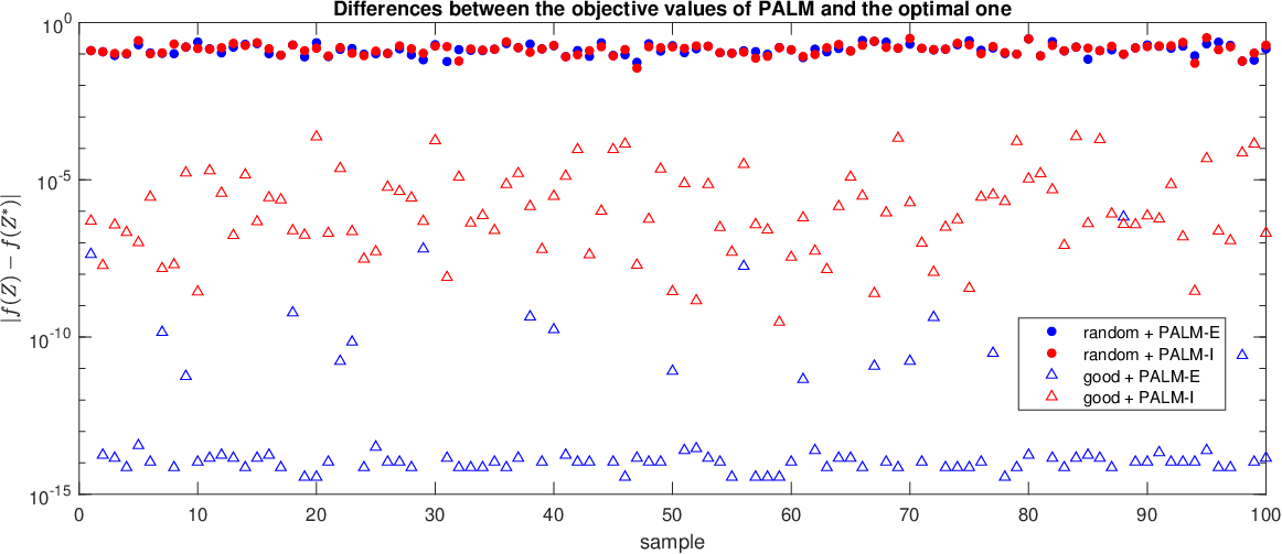
We can observe that, starting with randomly generated initial points, PALM-E and PALM-I often stop at points of similar qualities.

We then conduct a performance comparison between PALM-E and PALM-I with good initializations. The good initial points could be generated by random perturbation around the discretized optimal solution $Z^{*}$ supplied in [8]. The built-in “rand” function is invoked again to generate 100 good initial points, whose quantity of deviation from $Z^{*}$ is at most $10^{-3}$ . We plot out the averaged history of the minimum achieved relative KKT violation for both PALM-E and PALM-I; see Figure 1 (right). Moreover, the average CPU time used by PALM-E is about 0.85 seconds, while that of PALM-I is only approximately 0.03 seconds. These reflect the considerable time advantage of PALM-I over PALM-E in a neighborhood of optimal solution. Incidentally, the infeasible nature of PALM-I does not ruin much the solution quality; the maximum absolute difference between the terminating objective value and the optimal one is merely $2.39\times 10^{-4}$ , and it is less than $10^{-5}$ on over 75% samples.

The numerical results in this subsection reflect that PALM-I converges well and is clearly more efficient than PALM-E even with infeasibility. The efficiency is brought by the infeasible subsolver ssncg, whose usage is ensured by our theoretical results.

6.2 Optimization with Nonlinear Constraints

The second class of testing problems involves nonconvex quadratic objective functions and multiple ellipsoidal constraints, having the form

\begin{array}[]{cl}\displaystyle\min_{\mathbf{z}}&\displaystyle\frac{1}{2}\left\langle\mathbf{z},A\mathbf{z}\right\rangle+\left\langle\mathbf{b},\mathbf{z}\right\rangle\\ \mathrm{s.}~\mathrm{t.}&\displaystyle\frac{1}{2}\left\langle\mathbf{x}_{i},B_{i}\mathbf{x}_{i}\right\rangle+\left\langle\mathbf{c}_{i},\mathbf{x}_{i}\right\rangle\leq 1,~i=1,\ldots,n\end{array}

(6.2)

where, for $i=1,\ldots,n$ , $m_{i}=m\in\mathbb{N}$ ; $A\in\mathbb{S}^{mn}$ , while $\{B_{i}\}_{i=1}^{n}\subseteq\mathbb{S}_{++}^{m}$ ; $\mathbf{b}\in\mathbb{R}^{mn}$ and $\{\mathbf{c}_{i}\}_{i=1}^{n}\subseteq\mathbb{R}^{m}$ . This problem class is related to several domains [11, 15, 19], as noted in 1.2. In our implementation, $A$ and $\mathbf{b}$ are generated by the built-in function “randn” in Matlab. To form $\{B_{i}=(b_{i,jk})\}_{i=1}^{n}$ , we adopt the construction in [9, 14]:

b_{i,jk}=10^{\frac{j-1}{m-1}\text{ncond}_{i}},~\text{if }j=k;~~0,~\text{otherwise}.

It is easy to see that $\text{ncond}_{i}\in\mathbb{R}_{++}$ controls the condition number and the spectrum of each $B_{i}$ is spread in $[1,10^{\text{ncond}_{i}}]$ .

We compare the performances of PALM-E, PALM-F, and PALM-I when solving equation 6.2 with $n=5$ and $m=500$ ; that is, the number of variables is $2500$ . We select $\{\text{ncond}_{i}\}_{i=1}^{n}=\{3.00,3.25,3.50,3.75,4.00\}$ . The vectors $\{\mathbf{c}_{i}\}_{i=1}^{n}$ are set to be all-zero so that all ellipsoids are concentric. The proximal parameter is fixed at $\sigma_{i}^{(k)}\equiv\sigma=1$ for $i=1,\ldots,n$ and $k\geq 0$ . The three algorithms are armed with different subsolvers. Specifically, both PALM-E and PALM-I invoke the self-adative alternating direction methods of multiplier proposed in [14] (sadmm); PALM-F uses the feasible hybrid projection algorithm in [9] (hp). Note that the iterates produced by sadmm are not necessarily feasible. For $i=1,\ldots,n$ and $k\geq 0$ , we terminate hp within PALM-F if

\|\mathbf{x}_{i}^{(k+1)}-\tilde{\mathbf{x}}_{i}^{(k)}+\lambda_{i,\textup{{hp}}}^{(k+1)}(B_{i}\mathbf{x}_{i}^{(k+1)}+\mathbf{c}_{i})\|\leq\frac{\eta}{2}\|\mathbf{x}_{i}^{(k+1)}-\mathbf{x}_{i}^{(k)}\|_{\infty}.

where $\eta=0.99\sigma$ , and $\lambda_{i,\textup{{hp}}}^{(k+1)}\geq 0$ estimates the multiplier associated with the ellipsoidal constraint. It is not difficult to verify that the above inexact criteria help produce iterates fulfilling the assumption in [13]. Regarding sadmm in PALM-E and PALM-I, the residual function $r_{i}(\mathbf{x}_{i}^{(k+1)},\lambda_{i,\textup{{sadmm}}}^{(k+1)},\tilde{\mathbf{x}}_{i}^{(k)})$ becomes

		$\displaystyle\max\left\{\left\langle\mathbf{x}_{i}^{(k+1)},\mathbf{x}_{i}^{(k+1)}-\tilde{\mathbf{x}}_{i}^{(k)}+\lambda_{i,\textup{{sadmm}}}^{(k+1)}(B_{i}\mathbf{x}_{i}^{(k+1)}+\mathbf{c}_{i})\right\rangle,0\right\}$
	$\displaystyle+$	$\displaystyle\left\\|\mathbf{x}_{i}^{(k+1)}-\tilde{\mathbf{x}}_{i}^{(k)}+\lambda_{i,\textup{{sadmm}}}^{(k+1)}(B_{i}\mathbf{x}_{i}^{(k+1)}+\mathbf{c}_{i})\right\\|_{\infty}$
	$\displaystyle+$	$\displaystyle\lambda_{i,\textup{{sadmm}}}^{(k+1)}\max\left\{-\left[\frac{1}{2}\left\langle\mathbf{x}_{i}^{(k+1)},B_{i}\mathbf{x}_{i}^{(k+1)}\right\rangle+\left\langle\mathbf{c}_{i},\mathbf{x}_{i}^{(k+1)}\right\rangle-\alpha_{i}\right],0\right\}$
	$\displaystyle+$	$\displaystyle\max\left\{\frac{1}{2}\left\langle\mathbf{x}_{i}^{(k+1)},B_{i}\mathbf{x}_{i}^{(k+1)}\right\rangle+\left\langle\mathbf{c}_{i},\mathbf{x}_{i}^{(k+1)}\right\rangle-\alpha_{i},0\right\},$

where $\lambda_{i,\textup{{sadmm}}}^{(k+1)}\in\mathbb{R}_{+}$ is an approximate dual solution given by sadmm. In PALM-E, we set $\{\varepsilon^{(k)}\equiv 10^{-6}\}_{k\geq 0}$ ; for PALM-I, we choose $\big\{\varepsilon^{(k)}=\max\{\frac{10^{-1}}{(k+1)^{\ell}},10^{-6}\}\big\}_{k\geq 0}$ with $\ell=0.75$ . As in the previous subsection, the three outer frameworks are stopped once the relative KKT violation is smaller than $10^{-5}$ .

We invoke the built-in “randn” function in Matlab to generate 100 random initial points and then draw the averaged history of the relative KKT violation for the three algorithms; see Figure 3 (left).

The respective average CPU times used by PALM-E, PALM-F, and PALM-I are approximately 30.15 seconds, 9.26 seconds, and 1.74 seconds. One can observe that PALM-I takes the strengths of the infeasible subsolver sadmm and stands out with the best performance. We also make a comparison among the terminating objective values of the three algorithms. Since for equation 6.2, the optimal values are inaccessible, we take those given by PALM-E as benchmark and inspect the absolute differences of PALM-F and PALM-I from PALM-E; see Figure 3 (right). It appears that, even equipped with an infeasible solver, PALM-I is capable of yielding objective values much closer than PALM-F to those of PALM-E.

7 Conclusions

We recognize by examples the indispensability of infeasible subsolvers in PALM whenever constraints are complicated and illustrate through numerical simulations that PALM-I can be far more efficient than PALM-E and PALM-F. The shortage of existing works on PALM-I motivates us to analyze its convergence properties, particularly in the presence of objective value nonmonotonicity. We achieve this by constructing a monotonically decreasing surrogate sequence. Moreover, an implementable inexact criterion for subsolvers is devised for practical usage.

Futural improvements can be anticipated in several lines. For example, one could incorporate nonsmooth regularization terms into objective function and handle infeasibility and nonsmoothness simultaneously. Besides, the assumptions, such as Hoffman-like error bound, may appear to be restrictive and call for further relaxation. Last but not least, it is worth investigating the convergence properties of PALM-I on problems with nonconvex constraints and designing implementable inexact criteria for those contexts.

References

[1] H. Attouch and J. Bolte, On the convergence of the proximal algorithm for nonsmooth functions involving analytic features, Math. Program., 116 (2009), pp. 5–16.
[2] H. Attouch, J. Bolte, P. Redont, and A. Soubeyran, Proximal alternating minimization and projection methods for nonconvex problems: an approach based on the Kurdyka-Łojasiewicz inequality, Math. Oper. Res., 35 (2010), pp. 438–457.
[3] D. P. Bertsekas, A note on error bounds for convex and nonconvex programs, Comput. Optim. Appl., 12 (1999), pp. 41–51.
[4] J. Bolte, A. Daniilidis, and A. Lewis, The Łojasiewicz inequality for nonsmooth subanalytic functions with applications to subgradient dynamical systems, SIAM J. Optim., 17 (2007), pp. 1205–1223.
[5] J. Bolte, S. Sabach, and M. Teboulle, Proximal alternating linearized minimization for nonconvex and nonsmooth problems, Math. Program., 146 (2014), pp. 459–494.
[6] S. Bonettini, M. Prato, and S. Rebegoldi, A block coordinate variable metric linesearch based proximal gradient method, Comput. Optim. Appl., 71 (2018), pp. 5–52.
[7] R. Chill, On the Łojasiewicz-Simon gradient inequality, J. Funct. Anal., 201 (2003), pp. 572–601.
[8] M. Colombo, L. D. Pascale, and S. D. Marino, Multimarginal optimal transport maps for one-dimensional repulsive costs, Canad. J. Math., 67 (2015), pp. 350–368.
[9] Y. Dai, Fast algorithms for projection on an ellipsoid, SIAM J. Optim., 16 (2006), pp. 986–1006.
[10] P. Frankel, G. Garrigos, and J. Peypouquet, Splitting methods with variable metric for Kurdyka-Łojasiewicz functions and general convergence rates, J. Optim. Theory Appl., 165 (2015), pp. 874–900.
[11] S. He, Z. Li, and S. Zhang, Approximation algorithms for homogeneous polynomial optimization with quadratic constraints, Math. Program., 125 (2010), pp. 353–383.
[12] Y. Hu, H. Chen, and X. Liu, A global optimization approach for multi-marginal optimal transport problems with Coulomb cost. arXiv preprint arXiv:2110.07352, Oct. 2021.
[13] X. Hua and N. Yamashita, Block coordinate proximal gradient methods with variable Bregman functions for nonsmooth separable optimization, Math. Program., 160 (2016), pp. 1–32.
[14] Z. Jia, X. Cai, and D. Han, Comparison of several fast algorithms for projection onto an ellipsoid, J. Comput. Appl. Math., 319 (2017), pp. 320–337.
[15] R. Kučera, Convergence rate of an optimization algorithm for minimizing quadratic functions with separable convex constraints, SIAM J. Optim., 19 (2008), pp. 846–862.
[16] K. Kurdyka, On gradients of functions definable in o-minimal structures, Annales de l’institut Fourier, Grenoble, 48 (1998), pp. 769–783.
[17] X. Li, A. Milzarek, and J. Qiu, Convergence of random reshuffling under the Kurdyka-Łojasiewicz inequality. arXiv preprint arXiv:2110.04926, Oct. 2021.
[18] X. Li, D. Sun, and K.-C. Toh, On the efficient computation of a generalized Jacobian of the projector over the Birkhoff polytope, Math. Program., 179 (2020), pp. 419–446.
[19] B. Liu, C. Jiang, G. Li, and X. Huang, Topology optimization of structures considering local material uncertainties in additive manufacturing, Comput. Methods Appl. Mech. Engrg., 360 (2020), p. 112786.
[20] S. Łojasiewicz, Une propriété topologique des sous-ensembles analytiques réels, Les équations aux dérivées partielles, 117 (1963), pp. 87–89.
[21] , Sur la géométrie semi-et sous-analytique, Annales de l’institut Fourier, Grenoble, 43 (1993), pp. 1575–1595.
[22] O. L. Mangasarian and R. D. Leone, Error bounds for strongly convex programs and (super)linearly convergent iterative schemes for the least 2-norm solution of linear programs, Appl. Math. Optim., 17 (1988), pp. 1–14.
[23] P. Ochs, Unifying abstract inexact convergence theorems and block coordinate variable metric iPiano, SIAM J. Optim., 29 (2019), pp. 541–570.
[24] G. Peyré and M. Cuturi, Computational optimal transport: with applications to data science, Found. Trends Mach. Learn., 11 (2019), pp. 355–607.
[25] B. T. Polyak, Introduction to Optimization, Translations Series in Mathematics and Engineering, Optimization Software, Inc., Publications Division, New York, 1987.
[26] M. J. D. Powell and Y. Yuan, A trust region algorithm for equality constrained optimization, Math. Program., 49 (1991), pp. 189–211.
[27] M. Razaviyayn, M. Hong, and Z.-Q. Luo, A unified convergence analysis of block successive minimization methods for nonsmooth optimization, SIAM J. Optim., 23 (2013), pp. 1126–1153.
[28] R. Rockafellar and R. Wets, Variational Analysis, vol. 317, Springer-Verlag Berlin Heidelberg, 1998.
[29] T. Sun, H. Jiang, L. Cheng, and W. Zhu, A convergence framework for inexact nonconvex and nonsmooth algorithms and its applications to several iterations. arXiv preprint arXiv:1709.04072, Sept. 2017.
[30] X. Wang, X. Yuan, S. Zeng, J. Zhang, and J. Zhou, Block coordinate proximal gradient method for nonconvex optimization problems: convergence analysis. http://www.optimization-online.org/DB_FILE/2018/04/6573.pdf, Apr. 2018.
[31] Y. Xu and W. Yin, A block coordinate descent method for regularized multiconvex optimization with applications to nonnegative tensor factorization and completion, SIAM J. Imaging Sci., 6 (2013), pp. 1758–1789.
[32] L. Yang, Proximal gradient method with extrapolation and line search for a class of nonconvex and nonsmooth problems. arXiv preprint arXiv:1711.06831, Nov. 2017.
[33] Y. Yang, M. Pesavento, Z.-Q. Luo, and B. Ottersten, Inexact block coordinate descent algorithms for nonsmooth nonconvex optimization, IEEE Trans. Signal Process., 68 (2019), pp. 947–961.

		$\displaystyle\text{\lx@cref{creftype\lx@tilde refnum}{forward 1}}+\text{\lx@cref{creftype\lx@tilde refnum}{backward 1}}\geq-L\sum_{j=1}^{i-1}\\|\Delta\mathbf{x}_{j}^{(k+1)}\\|^{2}-L\sum_{j=1}^{i-1}\left\\|\begin{pmatrix}\mathbf{x}_{<j}^{(k+1)}-\bar{\mathbf{x}}_{<j}^{(k+1)}\\ \bar{\mathbf{x}}_{[j,i)}^{(k+1)}-\mathbf{x}_{[j,i)}^{(k+1)}\\ \bar{\mathbf{x}}_{i}^{(k)}-\bar{\mathbf{x}}_{i}^{(k+1)}\\ \bar{\mathbf{x}}_{>i}^{(k)}-\mathbf{x}_{>i}^{(k)}\end{pmatrix}\right\\|\\|\Delta\mathbf{x}_{j}^{(k+1)}\\|$
	$\displaystyle=$	$\displaystyle-L\sum_{j=1}^{i-1}\\|\Delta\mathbf{x}_{j}^{(k+1)}\\|^{2}-L\left\\|\begin{pmatrix}\mathbf{x}_{<i}^{(k+1)}-\bar{\mathbf{x}}_{<i}^{(k+1)}\\ \bar{\mathbf{x}}_{i}^{(k)}-\bar{\mathbf{x}}_{i}^{(k+1)}\\ \bar{\mathbf{x}}_{>i}^{(k)}-\mathbf{x}_{>i}^{(k)}\end{pmatrix}\right\\|\sum_{j=1}^{i-1}\\|\Delta\mathbf{x}_{j}^{(k+1)}\\|$
	$\displaystyle\geq$	$\displaystyle-L\sum_{j=1}^{i-1}\\|\Delta\mathbf{x}_{j}^{(k+1)}\\|^{2}-L\left\\|\begin{pmatrix}\mathbf{x}_{<i}^{(k+1)}-\bar{\mathbf{x}}_{<i}^{(k+1)}\\ \bar{\mathbf{x}}_{i}^{(k)}-\bar{\mathbf{x}}_{i}^{(k+1)}\\ \bar{\mathbf{x}}_{>i}^{(k)}-\mathbf{x}_{>i}^{(k)}\end{pmatrix}\right\\|\sqrt{(i-1)\sum_{j=1}^{i-1}\\|\Delta\mathbf{x}_{j}^{(k+1)}\\|^{2}}$
	$\displaystyle\geq$	$\displaystyle-\frac{L[\nu(i-1)+2]}{2}\sum_{j=1}^{i-1}\\|\Delta\mathbf{x}_{j}^{(k+1)}\\|^{2}-\frac{L}{\nu}\left[\\|\bar{\mathbf{x}}_{i}^{(k+1)}-\mathbf{x}_{i}^{(k)}\\|^{2}+\\|\Delta\mathbf{x}_{i}^{(k)}\\|^{2}\right]$
		$\displaystyle-\frac{L}{2\nu}\left[\sum_{l<i}\\|\Delta\mathbf{x}_{l}^{(k+1)}\\|^{2}+\sum_{l>i}\\|\Delta\mathbf{x}_{l}^{(k)}\\|^{2}\right],$

		$\displaystyle\big\\|\nabla_{i}f(\bar{\mathbf{z}}^{(k+1)})-\nabla_{i}f(\mathbf{x}_{<i}^{(k+1)},\bar{\mathbf{x}}_{i}^{(k+1)},\mathbf{x}_{>i}^{(k)})-\sigma_{i}^{(k)}(\bar{\mathbf{x}}_{i}^{(k+1)}-\mathbf{x}_{i}^{(k)})\big\\|$
	$\displaystyle\leq$	$\displaystyle L\left\\|\begin{pmatrix}\bar{\mathbf{x}}_{<i}^{(k+1)}-\mathbf{x}_{<i}^{(k+1)}\\ \bar{\mathbf{x}}_{>i}^{(k+1)}-\mathbf{x}_{>i}^{(k)}\end{pmatrix}\right\\|+\sigma_{i}^{(k)}\\|\bar{\mathbf{x}}_{i}^{(k+1)}-\mathbf{x}_{i}^{(k)}\\|$
	$\displaystyle\leq$	$\displaystyle L\left[\\|\Delta\mathbf{z}^{(k+1)}\\|+\\|\bar{\mathbf{z}}^{(k+1)}-\mathbf{z}^{(k)}\\|\right]+\sigma_{i}^{(k)}\\|\bar{\mathbf{x}}_{i}^{(k+1)}-\mathbf{x}_{i}^{(k)}\\|,$

		$\displaystyle\sqrt{c(\gamma-1)L}\sum_{k=s}^{t}\\|\bar{\mathbf{z}}^{(k+1)}-\mathbf{z}^{(k)}\\|$
	$\displaystyle\leq$	$\displaystyle\frac{c\bar{M}}{p}\left[\sum_{k=s-1}^{t}\\|\bar{\mathbf{z}}^{(k+1)}-\mathbf{z}^{(k)}\\|+\sum_{k=s}^{t}\\|\Delta\mathbf{z}^{(k)}\\|\right]+\frac{\bar{C}_{1}^{\bar{\theta}}}{p}\sum_{k=s}^{t}(e^{(k)})^{\bar{\theta}}+p\mathrm{D}^{(s,t+1)}$
	$\displaystyle\leq$	$\displaystyle\frac{c\bar{M}}{p}\left[\sum_{k=s-1}^{t}\\|\bar{\mathbf{z}}^{(k+1)}-\mathbf{z}^{(k)}\\|+\omega\sum_{k=1}^{\infty}\varepsilon^{(k)}\right]+\frac{\bar{C}_{1}^{\bar{\theta}}}{p}\sum_{k=1}^{\infty}(e^{(k)})^{\bar{\theta}}+p\bar{\varphi}(v^{(s)}-\overline{F}),$