An End-to-End Analysis of EMFI on Bit-sliced Post-Quantum ImplementationsDOI: XXXXXXX.XXXXXXXJournal: TECSCCS: Security and Privacy Post-Quantum Lattice-Based CryptographyCCS: Security and Privacy Digital SignaturesCCS: Security and Privacy Fault Attacks and Countermeasures
Abstract.
Bit-slicing is a software implementation technique that treats an N-bit processor datapath as N parallel single-bit datapaths. The natural spatial redundancy of bit-sliced software can be used to build countermeasures against implementation attacks. While the merits of bit-slicing for side-channel countermeasures have been studied before, their application for protection of post-quantum algorithms against fault injection is still unexplored. We present an end-to-end analysis of the efficacy of bit-slicing to detect and thwart electromagnetic fault injection (EMFI) attacks on post-quantum cryptography (PQC). We study Dilithium, a digital signature finalist of the NIST PQC competition. We present a bit-slice-redundant design for the Number-Theoretic Transform (NTT), the most complex and compute-intensive component in Dilithium. We show a data-redundant countermeasure for NTT which offers two concurrent bits for every single bit in the original implementation. We then implement a full Dilithium signature sequence on a 667 MHz ARM Cortex-A9 processor integrated in a Xilinx Zynq SoC. We perform a detailed EM fault-injection parameter search to optimize the location, intensity and timing of injected EM pulses. We demonstrate that, under optimized fault injection parameters, about 10% of the injected faults become potentially exploitable. However, the bit-sliced NTT design is able to catch the majority of these potentially exploitable faults, even when the remainder of the Dilithium algorithm as well as the control flow is left unprotected. To our knowledge, this is the first demonstration of a bitslice-redundant design of Dilithium that offers distributed fault detection throughout the execution of the algorithm.
Keywords:
Dilithium, Bit-slicing, Intra-Instruction Redundancy, Fault Attack Countermeasure, ARM Cortex-A9, Electromagnetic Fault Injection1. Introduction
Due to advancements in Quantum Computing and the discovery of Shor’s algorithm (Shor 1994), there is a looming threat to our existing public key infrastructure (PKI). With the possibility of powerful and large-scale quantum computers in not too distant future, common RSA- and ECC-based protocols become vulnerable.
NIST recently initiated a Post-Quantum Cryptography (PQC) Standardization process to select and standardize quantum-resistant algorithms (Moody et al. 2020) for Public Key Encryption (PKE), Key Establishment Mechanisms (KEM) and Digital Signatures (DS) in order to replace RSA and ECC schemes. This process is currently in its third and final round which has three finalist candidates in DS scheme category: Dilithium, Falcon and Rainbow (Moody et al. 2020). The criterion that determines the selection process includes classical as well as post-quantum (PQ) security guarantees. For the final round, in addition to key selection criterion such as classical security, theoretical PQ security guarantees, implementation cost and performance; resistance against active and passive implementation attacks, one of the most important criteria (Moody et al. 2020). Several authors have reported physical attacks on structured lattice-based schemes through exploitation of a number of side-channels such as power (Pessl 2017; Primas et al. 2017; Pessl and Primas 2019; Ravi et al. 2018; Aysu et al. 2018; Xu et al. 2021; Chen et al. 2021), electromagnetic emissions (Espitau et al. 2017b), cache timing (Groot Bruinderink et al. 2016; Pessl et al. 2017) and induced faults (Bruinderink and Pessl 2018; Bindel et al. 2016; Xagawa et al. 2021; Valencia et al. 2018; Espitau et al. 2017a; Ravi et al. 2019b; Pessl and Prokop 2021; Ravi et al. 2018; Ravi et al. 2019a).
In real-world usage scenarios, DS schemes will be deployed on a wide variety of platforms, including personal computers (PCs) and resource-constrained devices. It is crucial to analyze whether DS primitives and their implementations are vulnerable against fault injection analysis. There are previous works that have analyzed fault vulnerabilities on deterministic variants of lattice-based schemes to recover a part of secret key and validated those fault vulnerabilities using electromagnetic fault injection (EMFI) (Ravi et al. 2019b; Ravi et al. 2019a) and clock fault injection (Bruinderink and Pessl 2018; Xagawa et al. 2021) attacks. Such attacks are not impeded by basic fault countermeasures such as assembly-level instruction duplication/triplication (Barenghi et al. 2010), algorithm-level temporal redundancy (Schmidt and Medwed 2012; Ciet and Joye 2005; Bar-El et al. 2006) and verification-after-sign (Ducas et al. 2018). A major problem with these time-based redundancy techniques is that due to modern fault-injection capabilities, an adversary can inject consistent faults in redundant sections of code or data that may lead to faults go undetected. An adversary with precise control over the timing of the fault injection could bypass verification-over-sign countermeasure when fault effects are modelled by an instruction-skip.
The Number Theoretic Transform (NTT) is a central computation step in many post-quantum schemes including Dilithium. It is used to efficiently perform polynomial multiplication. Recent work has demonstrated that NTT can be used as a side-channel target leading to full-key recovery based on a single trace (Primas et al. 2017; Pessl and Primas 2019). To defend against such single-trace attacks on NTT, Ravi et al. proposed masking and shuffling countermeasures (Ravi et al. 2020). The performance overhead of their countermeasure for Dilithium’s key generation and signature generation procedures are in the range 12-197% and 32-490% respectively. However, this scheme has not been designed with controlled fault injection in mind.
Clearly, there is a need for comprehensive and fine-grained countermeasures to simultaneously protect lattice-based schemes against fault-injection and side-channel attacks while incurring tolerable performance costs. Bit-slicing has been proposed as a concrete software countermeasure against combined fault attacks and side-channel attacks using Intra-Instruction Redundancy (IIR) (Patrick et al. 2016; Kiaei et al. 2021; Breier et al. 2021) and higher-order masking (Kiaei et al. 2021) respectively.
As a first step, we present a bit-sliced design for the most critical sub-block in lattice-based schemes, NTT/INTT. We do so by representing the FFT-like structure of the NTT as parallel butterfly operations in each stage of NTT and then iterating over all the stages to compute final NTT output. We further exploit this bit-sliced design to provide a spatial intra-instruction redundant NTT design to protect it against faults in the datapath. We incorporate our countermeasure over the unprotected reference implementation of Dilithium Round 3 11 1 https://github.com/pq-crystals/dilithium. There is no prior work of fault attacks on the non-deterministic version of Dilithium (Round 3). To experimentally evaluate the effectiveness of the proposed countermeasure, we perform EMFI attack on an ARM Cortex-A9 processor-based Zynq SoC running Dilithium protected with our countermeasure.
1.1. Our Contribution
- (1)
We propose a software countermeasure based on dual data-redundancy obtained through our novel bit-sliced design for NTT in order to detect computation faults. While the use of bit-slicing with Intra-Instruction Redundancy (IIR) in context of fault attacks is not new (Kiaei et al. 2021), it’s application in the context of lattice-based post-quantum algorithms is still unexplored.
- (2)
The proposed countermeasure is generic and can easily be ported to other lattice-based post-quantum schemes having polynomial multiplications in abundance.
- (3)
We analyze the security of the proposed countermeasure to formulate estimated fault coverage in Dilithium.
- (4)
We evaluate the effectiveness of the proposed countermeasure on ARMv7-a architecture by testing it against EMFI attack on an 667 MHz ARM-based SoC.
- (5)
We perform a systematic search of the EM fault-injection parameters space, including precise location on the target chip, and optimal ranges for EMFI Pulse Delay and Pulse Power. We are able to increase the percentage of potentially exploitable faults to 10% of the fault injection attempts. From those potentially exploitable faults, we also determine that about 62% of them directly affect the data flow. This is possible due to the data-redundant design of our countermeasure to detect all data faults.
1.2. Outline
In Section 2, we will introduce the related literature and relevant background knowledge. Section 3 presents our bit-sliced design for NTT/Inverse NTT and our fault attack countermeasure design based on dual data-redundant bit-slicing. We state our assumptions about attacker’s capabilities and fault model in Section 4. Security analysis of the proposed countermeasure is provided in Section 5. Section 6 provides performance, footprint, overhead and a top-down EMFI analysis of our proposed countermeasure on an ARM-based SoC. Finally, we conclude this paper in Section 7.
2. Background
This section summarizes important background knowledge concepts, including bit-slicing, intra-instruction redundancy, Electromagnetic fault injection, and the NTT.
2.1. Bit-slicing
Bit-slicing is a software optimization technique originally developed to produce high throughput software implementations (Biham 1997). It was since also been applied as a side-channel and fault attack countermeasure (Belaïd et al. 2020; Patrick et al. 2016). Bit-sliced code is created from a boolean (bit-level) program. Bit-sliced programs are written using bit-wise logical operations (AND, OR, NOT, XOR) and as a result they run with bit-level parallelism and can be viewed as follows. An -bit variable in bit-sliced code with bits is spread over registers , such that register holds bit . A bit-sliced program on an -bit processor computes instances of -bit variable in parallel because it is composed of parallel copies of the boolean program. This -fold parallelism can be exploited in NTT computations since each stage of a -point NTT consists of independent butterfly operations. NTT operation is mapped to bit-sliced code by computing instances of butterfly operation per stage in parallel. Applying this bit-sliced butterfly computation over total stages will result in a -point NTT output.
2.2. Bit-slicing with Intra-Instruction Redundancy
Patrick et al. proposed a generic fault-attack countermeasure which requires an algorithm to be bit-sliced. We define slice as the bit-location in all registers which together constitute a -bit variable in bit-sliced code. The parallel bit-slices are used to create redundant copies of original data, which creates data redundancy within the execution of a single bit-wise instruction (Patrick et al. 2016). The resulting intra-instruction redundancy thus covers data bits within the same instruction. To detect faults, the original data slices and its respective redundant slices perform computation on same inputs and at the end of computation, they produce same outputs if there is no fault.
Intra-instruction redundancy builds on the fact that typical fault injection mechanisms offer poor control over the fault injection location. Therefore, it is difficult to affect the redundant copies within a single word in the same manner. Patrick also discusses an extension of intra-instruction redundancy which protects the control flow of an implementation, ie. the sequence and semantics of bit-wise instructions. In this approach, the different bit-slices allocate time-redundant copies of data bits, such a redundant copy of a data bit belonging to different iterations of an algorithm.
2.3. Fault Injection Mechanisms
Active Fault Attacks (FA) are a well-known threat to embedded devices. In this type of attack, the attacker tries to inject faults in the normal computation by pressuring the underlying device out of its nominal operating conditions. Faulty ciphertext, or fault signatures, can then be used to improve the cryptanalysis.
Fault injection is a relevant threat to post-quantum cryptography. The deterministic signature of Dilithium was shown susceptible to a Differential Fault Analysis (DFA) (Bruinderink and Pessl 2018), and recently also the randomized signature of Dilithium was shown vulnerable to a Signature Correction Attack (Islam et al. 2022).
We discuss some related work relevant to the EM fault injection mechanism used in our work. EMFI attacks produce a local transient magnetic field near the device which induces transient faults into the device computation. This could leak sensitive device information, cause data corruption (Menu et al. 2019), change the program flow (Rivière et al. 2015), bypass security mechanisms such as secure boot (Cui and Housley 2017) or cause privileged escalation (Gaine et al. 2020). Our research specifically considers EMFI on ARM architectures. Early work on EMFI is presented in (Dehbaoui et al. 2012; Schmidt and Hutter 2007). Moro et al. introduced for the first time a precise fault model to study the impact of an EM fault injection on a 32-bit ARM micro-controller (Moro et al. 2013). Elmohr et al. shows that EMFI is more susceptible at lower supply voltages and higher clock frequencies on ARM and RISC-V platforms and multi-instruction skips are possible with a single EM pulse (Elmohr et al. 2020). Rivière et al. performed EM fault injection on cache of an ARM Cortex-M4 micro-controller (Rivière et al. 2015). Menu et al. presents an EMFI attack on the data-prefetch mechanism of an ARM micro-controller to achieve AES key recovery and AES key resetting with a single fault injection (Menu et al. 2019). Majeric et al. successfully injected EM-induced faults into an ARM Cortex-A9 based SoC targeting an AES hardware accelerator (Majéric et al. 2016).
2.4. Definition of NTT and Inverse NTT
Dilithium uses NTT for efficient polynomial multiplication which is the key part of the scheme and the focus of this work. In this section, we provide the definition of NTT and inverse NTT. Detailed explanation of the structure of Dilithium algorithm can be found in the original specification (Ducas et al. 2018).
NTT is a generalized version of well-known Fast-Fourier Transform (FFT) where all the arithmetic is performed in the prime finite field instead of complex numbers. In ideal lattice-based cryptography, main operation is polynomial multiplication in the ring , where, ring denotes the set of polynomials with integer coefficients modulo and denotes the ring of polynomials with integer coefficients from the ring reduced by a cyclotomic polynomial . NTT-based polynomial multiplication requires that is a power of two and the modulus is chosen to be a prime such that . This way contains a primitive -th root of unity and its square root , which means that .
Let two polynomials with coefficients and respectively. Then, polynomial multiplication is defined as
| (1) |
where, denotes the point-wise multiplication of polynomials. To eliminate the overhead of zero-padding and to length , negative-wrapped convolution property of NTT is used. So, the transformation generates a polynomial whose coefficients can be defined as
| (2) |
The inverse NTT is computed in exactly same way except that is replaced with and the final results are scaled by factor. The inverse NTT transforms the polynomial back to whose coefficients are obtained as
| (3) |
3. Proposed Bit-sliced design of NTT-based Polynomial Multiplication
We propose to use bit-slicing technique on NTT and then utilize this bit-sliced NTT design to construct a data-redundant countermeasure for NTT to provide fault-attack resistance. We have implemented our bit-sliced NTT/INTT design and integrated it with reference Dilithium implementation in C. In this section, we describe the bit-sliced code generation process, the bit-sliced design of key components of Dilithium and the bit-sliced dual data-redundant countermeasure design for NTT/INTT.
3.1. Bit-sliced code generation process
Bit-slicing requires a boolean program (bit-level program), which is difficult to program because only single-bit operations can be used. To simplify the development of this boolean program, we express its equivalent functionality at the Register-Transfer Level (RTL) in a hardware description language, and then use logic synthesis to convert this behavior into an equivalent description of boolean operations. We have automated this step into an open-source logic synthesis environment that creates a bit-slice program in C directly from an RTL description in Verilog (Kiaei and Schaumont 2021).
Figure 1 shows register-transfer level description of standard Cooley-Tukey butterfly unit. This Butterfly unit forms the foundation block of NTT transforms and is built from a -bit modular adder, a -bit modular subtractor and a -bit modular multiplier module with modular operations in , where, prime modulus parameter is fixed to ( bits) for Dilithium algorithm. Modular reduction in adder and subtractor is performed using conditional subtraction and addition respectively. While design of modular reduction in multiplier is based on barret reduction algorithm (Barrett 1986) as described in Algorithm 6 (Banerjee et al. 2019). Butterfly operation takes three -bit signed integers as input: , and twiddle factor . The Butterfly operation then computes and resulting in two outputs and respectively.
The Verilog RTL description for the butterfly unit is first converted to a boolean program, a gate-level netlist comprised of primitives such as AND, OR, NOT and XOR using logic synthesis. This boolean program is further converted into a C code by levelling the gates in the netlist and each gate is substituted with an equivalent bit-wise logical instruction. This C code generation is integrated as a backend pass in YOSYS, the open-source synthesis tool (Wolf 2012). Listing 1 illustrates the generated bit-sliced C code. Each input or output in Figure 1 is mapped into a corresponding int32_t representing 32 parallel slices. The input argument is passed a zero value since the butterfly unit is essentially a combinational circuit thus requires no state preservation across multiple calls to bit-sliced function. To execute this bit-sliced code, the inputs must be converted into bit-sliced format. This requires doing matrix transposition of 32 -bit inputs into 32-bit registers, for example, holds the bit of 32 different inputs. Once the bit-sliced computation is done, outputs are reverse-transposed from bit-sliced format into normal format.

3.2. Bit-sliced Components of Dilithium
In this section, we describe the mapping of key building blocks of Dilithium such as forward and inverse NTT transformations (NTT and INTT), polynomial multiplication and matrix-vector Polynomial Multiplication to bit-sliced code. We target bit-slicing to those sections of code of the Dilithium algorithm which are both computationally intensive and vulnerable with respect to fault attacks (Bruinderink and Pessl 2018; Ravi et al. 2018; Ravi et al. 2019a), side-channel attacks (Primas et al. 2017; Pessl and Primas 2019) and cache-timing attacks (Facon et al. 2018). Bit-slicing provides constant-time implementation, enables intra-instruction redundancy to protect against fault-attacks and higher-order masking to protect against power side-channels (Kiaei et al. 2021). Please refer Algorithms 1 and 2 where the FA protected polynomial multiplication and matrix-vector polynomial multiplication instances are highlighted in blue.
3.2.1. Bit-sliced NTT and Inverse NTT
We exploit the iterative nature of NTT algorithm to apply fine-grained parallelism through bit-slicing. The NTT/INTT of size is typically computed in total stages with each stage consisting of butterfly operations. Dilithium algorithm operates with polynomials of size and uses 256-point NTT and 256-point INTT to compute polynomial multiplication. Cooley-Tukey (CT) butterfly structure is used to perform both NTT and INTT operations. The CT butterfly-based NTT and INTT requires inputs in bit-reversed order and generates outputs in normal order, similar to the decimation-in-time (DIT) FFT. While the INTT operates similar to NTT expect that its twiddle factors are negative powers of and coefficient-wise multiplication of output by and powers of as defined in Equations 2 and 3. In order to map 256-point NTT to bit-sliced mode, 256-point NTT is broken down into four 64-point NTTs. Now, each 64-point NTT computation takes six stages and each stage has 32 butterfly operations. Since all butterflies within any stage of the NTT can be computed independent of one another, this allows us to apply bit-sliced approach to NTT architecture. To parallelize the 32 butterfly operations in any stage of 64-point NTT, it is computed using a single call to bit-sliced butterfly function butterflyCompute() as defined in Listing 1.
Figure 2 shows the step-wise transformation of an input polynomial a into 256-point NTT output polynomial using bit-slicing technique, whereas, Algorithm 3 outlines its pseudocode. In lines 25-43 of the pseudocode, bit-sliced manipulation process takes place using SIMD instructions explained later in the section, we use ARM NEON intrinsics to support for Cortex-A series processors. This particular section of code can easily be ported to support AVX2 SIMD instructions for Intel CPUs as well. The NTT transformation starts with PolyBitReversal step which performs bit reversal on the input polynomial :
| and nS |
The bit-reversed input polynomial is then bisected and stored into arrays and as the two set of inputs applied to the 128 butterflies in the first stage of 256-point NTT as shown in lines 8 - 11 of code. Each array represents 4 subsets each of size and one subset drawn from each array therefore forms the 64 inputs to a 64-point NTT block. In other words, first subset and second subset constitutes the first inputs and second inputs respectively for the 32 butterflies of a 64-point NTT. These two butterfly inputs subsets can be viewed as and respectively in the Figure 3a. Before -bit input polynomial coefficients can be processed by a bit-sliced function, the input has to be transposed. The PolyTranspose step in Figure 2 performs transpose on the two butterfly inputs arrays and converts 32-bit inputs per first and second subset into 32 -bit inputs each as depicted by red and green colored slices respectively in the Figure 3a. In Figure 4, the transposed butterfly inputs subsets and are then passed as input arguments to pointwisemultiplier() bit-sliced function at PowMulψ step of Figure 2 to realize multiplication of polynomial coefficients with respective powers of negative convolution () factors. Its output subsets and are then inputs to butterflyCompute() bit-sliced function resulting in two butterfly outputs subsets, and , at the same time, comprising of the 32 first outputs and 32 second outputs respectively for the 32 butterflies in stage of a 64-point NTT block. In Figure 4, the 32 alternate red and green slices in two butterfly outputs subsets represents intermediate outputs which become the first inputs and second inputs respectively to the stage butterflies of a 64-point NTT. In order to process stage inputs by butterflyCompute() function, all the first butterfly inputs represented by red slices should be placed together in one subset and all the second butterfly inputs represented by green slices should to be placed together in the other subset. We therefore perform bit-sliced manipulation operation after bit-sliced butterfly computation operation in first five stages of 64-point NTT to obtain the desired butterfly inputs subsets for next stage as shown in the Figure 4. We exploit the fact that NTT is easily vectorizable hence bit-sliced manipulation takes the two input subsets through a sequence of SIMD bit-wise operations as shown in the lines 25-43 of pseudocode and can also be perceived as a gate-level circuit illustrated in Figure 4. This process begins with masking the inter-mixed red slices and green slices in both the subsets with a given mask value and its complement respectively. To extract and set together the red slices from both the subsets, the SIMD ANDed output of red slices from second subset with a complementary mask value is shifted by a given shift value and finally, it is SIMD ORed with the SIMD ANDed output of red slices from first subset with mask value. The results of bit-sliced manipulation are stored back into same memory locations from where butterfly inputs are read. Mask value, , complementary mask value, and shift value, are configured for first five stages of 64-point NTT stage since the number of overlapping butterflies differs stage-wise. Figure 4 highlights the path with red and green which combines all red slices together and green slices together respectively. Last stage of 64-point NTT does not require bit-sliced manipulation operation because all the 32 butterflies are interleaved with each other which causes both the butterfly output subsets to already have all the first butterfly outputs in one subset and all the second butterfly outputs in the other subset. A 64-point NTT output in bit-sliced domain is represented in Figure 5 using a rectangular block with top-half/red portion occupied with 32 first outputs (in 32 adjacent red slices spread across 32 words) and bottom-half/green portion occupied with 32 second outputs (in 32 adjacent green slices spread across 32 words) of 32 butterflies in the stage.
To compute the stage of 256-point NTT, 4 64-point NTT blocks are combined to form 2 128-point NTT blocks by 4 invocations to butterflyCompute() bit-sliced function as in lines 52-55 of pseudocode. Figure 5 shows that red portions and green portions of top two 64-point NTT blocks are inputs for the first 32 butterflies and next 32 butterflies respectively in the 7th stage of 256-point NTT which combine together to produce first 128-point NTT block. Butterfly outputs are stored back into same memory locations where the inputs are in. Going to the stage, composition of 2 128-point NTT blocks leads to a single 256-point NTT block which is computed by 4 invocations to butterflyCompute() bit-sliced function as in lines 63-66 of pseudocode. We get the final 256-point NTT output by performing last step in Figure 2, ReverseTranspose to convert the 32-bit 256-point NTT outputs from bit-sliced domain to normal domain.
It is to be noted that we use pre-computed transposed twiddle factors: , and , in our bit-sliced implementation of 256-point NTT and INTT. The bit-sliced implementation for 256-point INTT is same as 256-point NTT except that there is PowMulψ step at the end before the ReverseTranspose step instead of the beginning to perform point-wise multiplication of INTT output polynomial coefficients with respective powers of using pointwisemultiplier() bit-sliced function.
3.2.2. Bit-sliced Polynomial Multiplication
An NTT-based multiplication of two polynomials is computed using two forward NTTs to transform the input polynomials, a point-wise vector multiplication and one inverse NTT as stated in Equation 1. Bit-sliced implementation of multiplication of two 256 elements polynomials uses bit-sliced instances of: 256-point NTT and 256-point INTT for forward and inverse transform; pointwisemultiplier() bitsliced function to perform point-wise multiplication of 2 polynomials in NTT domain representation.
3.2.3. Bit-sliced Matrix-Vector Polynomial Multiplication
Bit-sliced multiplication of a polynomials matrix with a polynomials vector is computed by calculating the inner product row-wise and the inner product is composed of bit-sliced polynomial multiplications and bit-sliced polynomial accumulations. pointwiseaccumulator() bit-sliced function uses a state element to accumulate over the polynomials resulting from the point-wise multiplication of NTT domain polynomials in a given row of a matrix with NTT domain polynomials of a vector. This state element is mapped into a global variable to preserve state across multiple invocations of pointwiseaccumulator() function. To accumulate polynomials, we run bit-sliced accumulation over their 32 coefficients using calls to pointwiseaccumulator() and by iterating bit-sliced accumulation over the size of the polynomial, it outputs a single polynomial in bit-sliced format which is then followed by a bit-sliced INTT transformation to get the final polynomial for that particular row.
3.3. Proposed Fault-Attack Countermeasure for Dilithium Algorithm
In this section, we describe the implementation of Fault-Attack Countermeasure based on IIR mechanism in Dilithium. We utilize the bit-sliced construction defined for key elements of Dilithium in Section 3.2 as the foundation to add dual spatial redundancy to it. We consider the case of 256-point NTT to demonstrate the IIR-based countermeasure in Dilithium. In bit-sliced implementation of 256-point NTT, each slice is allocated to operate on a different coefficient of a polynomial for maximum throughput. We separate slices into original data slices (ODS) and redundant data slices (RDS) occupying the lower-half and upper-half word respectively for fault detection. RDS and ODS operate on the same input coefficients at any intermediate stage of 256-point NTT, and thus, they produce same output if no fault occurs. If a fault occurs during their execution, then it will be detected when output polynomial coefficients are compared at the end of 256-point NTT transformation.

Polynomial coefficients array of size arranged in bit-reversed order is split into 16 subsets each of size such that each subset has first half elements as polynomial coefficients and remaining are its copies. While half of the subsets store coefficients which are first inputs and remaining half subsets have second inputs of butterflies in first stage of 256-point NTT. Then, at PolyTranspose step, subsets are transposed into bit-sliced format having dual-spatial redundancy. Figure 3b illustrates a part of PolyTranspose step, when one of the first butterfly inputs subsets and one from the second butterfly inputs subsets, both shown in blue, are converted into their transposed versions represented by red and green respectively wherein the redundant slices and original data slices are portrayed in different patterns and indicated by arrows. All slices are split across 32 words for 32-bit polynomial coefficients. In next step, transposed subsets are point-wise multiplied with their respective power of factors using pointwisemultiplier() bit-sliced function.
Next, when a first butterfly inputs subset and a second butterfly inputs subset are passed to butterflyCompute() bit-sliced function, half of the butterflies will operate on redundant inputs, thus produces two butterfly output subsets with redundant slices which then become inputs to next stage. This leads us to compute in-parallel two 32-point NTTs, original and its copy, with 16 butterflies and its copies being computed per stage using a single call to butterflyCompute(). Here also, each stage except the last one involves bit-sliced manipulation process after butterflyCompute similar to non-redundant bit-sliced implementation. With dual data-redundancy, bit-sliced 256-point NTT is broken down into 8 32-point NTT blocks instead of 4 64-point NTT blocks. These 8 32-point NTT blocks are computed on 8 different pairs of butterfly inputs subsets and each 32-point NTT output in transposed form is represented in Figure 6 using a rectangular block with top-half/red portion and bottom-half/green portion storing first butterfly outputs and second butterfly outputs respectively of last stage of a 32-point NTT block. So, stage of 256-point NTT will merge these 8 32-point NTT blocks into 4 64-point NTT blocks using 8 calls to butterflyCompute() function in a way as illustrated in Figure 6. In stage, 4 64-point NTTs combine to output 2 128-point NTT blocks. 2 128-point blocks combine to output final 256-point NTT output. It is to be noted that in each stage, NTT blocks are generated along with its copies in-parallel.
An adversary can bypass this countermeasure by injecting two single-bit faults that are in different halves of the processor word. These two faults have to align with any of the ODS and its respective RDS. Then, both will produce same faulty 256-point NTT output, going undetected.
4. Fault Attacker Model
We assume that an attacker has complete physical access to the device during the execution of the signature generation procedure. The attacker should be able to collect the signatures generated by a message of his/her choice. The attacker should either be able to have a trigger in the device to time its fault injection or capability to capture power/EM traces to extract from them the timing information of points of interest. The attacker can stress the circuit or environmental conditions using an EM glitch. These glitches will induce localized transient faults into the device computation. An attacker can modify an instruction to be executed affecting the program flow of the algorithm or can cause algorithm modification depending upon the replaced instruction. An attacker can also modify the data to be loaded from memory without modifying the load instruction itself.
Proy et al. investigated effects of EM-induced faults at Instruction Set Architecture (ISA) level on an ARM Cortex-A9 based SoC (Proy et al. 2019). They have identified varied fault models ranging from instruction skip and register corruption, widely-adopted fault model for micro controllers (Rivière et al. 2015; Ravi et al. 2019b), to operand substitution, multiple correlated register corruptions and advanced control flow hijacking for SoCs. In this work, we have not performed characterization of fault effects rather assumed the studied fault effects on SoCs in previous works (Proy et al. 2019; Trouchkine et al. 2019).
5. Security Analysis of the Proposed Countermeasure
In this section, we provide the security analysis of the proposed countermeasure in Section 3.3 against the fault attacker models defined in Section 4.
In the unprotected, Dilithium implementation, any computation or instruction fault during the execution of signature generation algorithm may be useful for the adversary. As there is no detection mechanism for this implementation, the faulty signatures given out by the signature generation process may lead to some information about the secret key. The simplest method to protect against faults is function level temporal redundancy, i.e., to run the signature generation multiple times and only return the signature if their results are equal. However, it doesn’t guarantee security in a case where adversary injects similar faults to multiple executions. Another efficient countermeasure technique to protect against faults is verification-after-sign but it cannot detect faults when injected into verification procedure such that it gives a pass to faulty signatures as valid signatures. While in presence of the proposed countermeasure, it thwarts the malicious attempt by detecting the data faults through redundant data slices. However, adversary can circumvent the countermeasure by injecting same faults in both the original data slices and their corresponding redundant data slices. If either an original data slice or its respective redundant data slice has an error, it is detected by taking their XOR and its expected value is non-zero. Whereas, in case of non-faulty operations, they will always produce a zero value. Since this fault-response generation step is not covered by IIR, they would be duplicated using conventional approaches to protect from instruction faults.
We investigate the fault coverage of the proposed countermeasure using performance hotspots analysis. To perform this measurement on ARM Cortex-A9, we use Xilinx Vitis TCF Profiler. Results of profiling the protected Dilithium algorithm are shown in Table 1. We observe that butterflyCompute() and pointwisemultiplier() bit-sliced functions are the largest contributors to CPU cycles with a CPU usage of and on ARM Cortex-A9 target platform. These two functions form the core of bit-sliced polynomial multiplications and protects the most time-consuming operations from data faults. Countermeasure also delivers a temporal fault coverage of about , thereby, significantly decreasing the attack surface of Dilithium Algorithm.
The proposed countermeasure doesn’t provide protection against memory faults like Rowhammer (Gruss et al. 2016). Typical countermeasure for such type of fault attacks is storing redundant copies of sensitive intermediate variables and verify its value before using it. Additionally, this countermeasure doesn’t protect against instruction skipping faults since both original data slices and their corresponding redundant data slices will have the same effect. So, rejection sampling step implemented as an if-condition remains unguarded and if skipped, may leak secret-dependent signatures.
| Active Functions | CPU Cycles (%) | No. of Calls |
|---|---|---|
| butterflyCompute | 58.6 | 16064 |
| pointwisemultiplier | 20.4 | 5360 |
| pointwiseaccumulator | 0.26 | 1024 |
6. Experimental Results
We perform performance & footprint evaluation, overhead analysis and experimental fault attack resistance evaluation of the proposed countermeasure. To inject faults, we use Electromagnetic Fault Injection (EMFI) setup as described in Section 6.1.

6.1. Experimental Fault Injection Setup
This section describes our measurement setup for EM Pulse Injection. The setup consists of a hardware part, device under attack, a software part and experimental process.
6.1.1. Hardware Setup:
The EM fault injection bench is composed of a control PC, the targeted device, an automated XYZ stage, a pulse generator, an oscilloscope and an EMFI transient probe. We use commercially available FI hardware and software tools (Riscure 2001) to build this setup. The target is placed on the XYZ stage as shown in the Figure 7. We use a classic EMFI probe tip made of a copper winding around a ferrite core. It has a flat-head tip of positive polarity and 1.5 mm diameter in order to cause disturbance in small part of the device. The probe is connected to the pulse generator and oscilloscope. Oscilloscope is used to measure the trigger and probe coil current signals. As soon as the probe receives a pulse from the pulse generator at its digital glitch input, it discharges the capacitor bank into the coil at the probe tip thereby creating a single EM pulse. The PC controls every part of the setup including configuring the injection parameters and capturing the results for analysis. The control software running on the PC synchronizes its operations with the other components of the setup through serial communication.
6.1.2. Device Under Attack:
The attack is realized on a Zynq-7000 SoC, XC7Z030SBG485 Flip-Chip Lidless BGA device having 19x19 mm package size. This SoC is embedded on Avnet PicoZed, our target board and it consists of a dual-core 32-bit ARM Cortex-A9 MPCore based processing system (PS) and Xilinx programmable logic (PL) on CMOS 28nm technology implementing the ARMv7-a ISA and runs by default at 667 MHz. The ARM processor has two separate 32 KB L1 caches for instruction and data, 256 KB on-chip memory and shares 512 KB L2 cache with NEON co-processor. The target board has 1 GB external DDR3 Memory and 128 MB QuadSPI Flash.
6.1.3. Software Setup:
The test program is booted from external flash in PS Master Boot Mode and is executed from DDR3. We used Xilinx Vitis platform to program flash and for on-chip hardware debugging. We power the target during all the experiments at nominal voltage. A trigger is implemented using a general purpose IO pin of the target. The test program running on the target sets this trigger signal high just before the beginning of attack window and then sets the trigger signal low after the window ends. The test program used for all the experiments is open-source reference C implementation of Dilithium Round 3 version integrated with our countermeasure. This implementation was compiled with the arm-none-eabi-gcc-9.2.0 using compiler flags -mcpu=cortex-a9 -mfpu=neon-vfpv3 -mfloat-abi=hard -O0. For every fault injection, the test program sends a fault response and complete signature at the end of execution to the PC over UART for faults classification.
6.1.4. Experimental Process:
We configure four injection parameters in our EMFI setup for getting and increasing the probability of a successful fault injection. Since the full parameter search space is huge to be exhaustively covered, we rather focus on searching the optimal values for the most important parameters and keeping remaining parameters fixed:
- •
Spatial location - The x-y position is defined as the 2D-position of injection probe relative to the reference points set on the top surface area of the chip. We keep the Z-position fixed at approximately 0.4mm from the top of the chip.
- •
Temporal location - The amount of time between the trigger is set high and the actual EM pulse injection. It is also referred to as EMFI Pulse Delay.
- •
Injection voltage - The Intensity of EM pulse. It configures the maximum voltage over the coil which effects the current induced into the chip. It is also referred to as EMFI Pulse Power and this value is a percentage of the highest injection voltage of the probe, which is 475V.
- •
Pulse duration - The amount of time the probe continuously supplies variable coil current. We fixed it to 500 kns.
In this setup, the probe tip coil emits a single EM pulse for a fault injection. First, we gather golden signature response from the target running a fault-free execution for a fixed message and seed. After that, for every EM fault injection measurement, output response from the target is compared against the non-faulty output. The result of the experiment can be classified and grouped into different categories:
- •
No Effect - When the target output matches the expected response; no observable effect of fault is seen.
- •
Crash - When the target results in error conditions which are handled by fault exceptions such as Data Abort, Pre-fetch Abort or an undefined instruction on ARM processors. For each of these exceptions, there is an exception handler set up with an infinite loop.
- •
Faults Not Detected - When the output signature response is different from the expected response but fault response is not detected.
- •
Faults Detected - When the output signature response is different from the expected response but fault response is detected.
We do a software reset of the target after every measurement so that the result state of the previous measurement doesn’t effect next measurement. After a reset, the target boots from flash and runs the test program automatically. In the crash cases, we do manual external reset of the target. Faulty signatures are those which pass the rejection checks in the signing procedure. In a real-world setting of the proposed countermeasure, when a fault is detected by our countermeasure, it would not output any faulty signature for secret key analysis by the attacker.
6.2. Performance Analysis
Table 2 shows the performance impact of the proposed bit-slicing based IIR countermeasure on the key operations of Dilithium on ARM Cortex-A9 target platform. We report results for the NIST security level 2 of Dilithium (Dilithium2). These numbers are median cycle counts for 10,000 executions of Dilithium, including key generation and signing procedures only, as verification operates on public information. Note that hardware performance counters are used to measure cycles count. All the implementations for performance analysis are compiled with -O3 optimization flag. Both the slowdowns are calculated by dividing by the corresponding unprotected Dilithium metric. For NTT/INTT, slowdown directly comes from the butterflyCompute() and pointwisemultiplier() bit-sliced functions since they involve a large number of data transfers as compared to compute cycles. Their contribution in runtime of Dilithium in terms of number of functions calls is shown in Table 1. It is observed that Dilithium key generation and signing incurs high performance overhead since a significant portion of their runtime is dominated by NTT/INTTs, thereby, leading to large call counts of these bit-sliced functions. From the Table 2, it should be noticed that protected version have almost twice the slowdown compared to the bit-sliced version since the protection is based on dual spatial redundancy.
| Dilithium Main Operations | Cycles Count | Slowdown () | |||
|---|---|---|---|---|---|
| Unprotected | Bitsliced | Protected | Bitsliced | Protected | |
| Forward NTT | 28,928 | 925,824 | 1,827,584 | 32.0 | 63.2 |
| Inverse NTT | 30,848 | 928,128 | 1,833,152 | 30.1 | 59.4 |
| Point-wise Multiplication | 4,864 | 302,144 | 547,904 | 62.1 | 112.6 |
| Full Multiplication | 93,888 | 3,082,496 | 6,037,888 | 32.8 | 64.3 |
| Key Generation | 2,231,872 | 32,030,400 | 57,659,968 | 14.4 | 25.8 |
| Signature Generation | 7,150,272 | 191,078,144 | 351,530,304 | 26.7 | 49.2 |
6.3. Footprint Analysis
Footprint is calculated by measuring the compiled program size. Table 3 shows the footprint results for unprotected, bit-sliced and protected Dilithium implementations. All the implementations for footprint analysis are compiled with -Os optimization flag. Increased memory requirements in .text memory section for bit-sliced implementation comes from the butterflyCompute(), pointwisemultiplier() and pointwiseaccumulator() bit-sliced functions which occupy 77020 bytes, 82708 bytes and 3672 bytes respectively of code segment on ARM Cortex-A9 platform. The code size of a bit-sliced function is directly proportional to the cycles it takes to execute due to its linear code structure. This is evident by the protection cost of Dilithium implementation when protected with our bit-slicing based countermeasure mentioned in Table 2. While pre-computed twiddle and convolution factors used in bit-sliced polynomial multiplication computations are also part of .text section. Bit-sliced implementation also shows an overhead in .bss memory section due to uninitialized global intermediate array variables of polynomial size used in bit-sliced NTT/INTT operations. Table 3 shows that the footprint overhead of protected Dilithium implementation on target platform is 2.09 times.
| Dilithium Implementation | Code Size (bytes) |
Overhead
() | |||
| .text | .data | .bss | Total | ||
| Unprotected | 48,572 | 1,144 | 145,544 | 195,260 | - |
| Bitsliced | 222,488 | 1,144 | 159,056 | 382,688 | 1.95 |
| Protected | 232,064 | 1,144 | 176,464 | 409,672 | 2.09 |
6.4. Overhead Analysis
Table 4 shows our analysis of different bit-sliced functions used in the Bit-sliced Dilithium implementation in terms of instruction breakdown and overhead of data movements. The overhead values reported are calculated as the number of LDR and STR instructions divided by the total number of instructions. We observe the number of ORR, EOR, AND, ADD and SUB instructions involved during the execution of butterflyCompute(), pointwisemultiplier() and pointwiseaccumulator() bit-sliced functions. Furthermore, we observe that moving data from memory to processor is expensive for these functions. The number and composition of logical bit-wise instructions originates directly from the Boolean gate-level netlist generated from the Verilog description. The overhead of LDR and STR instructions, however, is introduced by the compiler due to increased register pressure. There is register pressure because net width in the netlist, i.e., the number of active variables in bit-sliced code exceeds the number of registers available in the underlying hardware. The overhead related to register spilling into memory is about 48-62% in terms of instruction count. This overhead explains the slower performance of the bit-sliced NTT, INTT, Full Multiplication and Matrix-Vector Multiplication operations of Dilithium.
|
Bit-sliced
function |
Instruction Mix | Overhead (%) | ||||||
|---|---|---|---|---|---|---|---|---|
| ORR | EOR | AND | ADD | SUB | LDR | STR | ||
| butterflyCompute | 1830 | 2957 | 3994 | 2 | 2 | 5210 | 3130 | 48.70 |
| pointwisemultiplier | 1931 | 3270 | 4331 | 2 | 2 | 5618 | 3295 | 48.31 |
| pointwiseaccumulator | 51 | 97 | 120 | 13 | 1 | 277 | 194 | 62.54 |
6.5. Fault Countermeasure Evaluation
In this section, our goal is to maximize the chances of obtaining a successful fault which gets detected by the proposed countermeasure. For this, determination of injection parameters is an essential step which consists of finding the spatial location, temporal location and injection voltage. We demonstrate the effectiveness of the proposed countermeasure by performing fault injection on protected NTT of , our point of interest in the test program and it is timed using a GPIO-based trigger as explained in Section 6.1. Protected NTT is divided into three phases: transpose, compute and reverse-transpose. As we know that redundant computations take place in the compute phase, therefore, we set compute phase as our attack window and it takes roughly 10M ns.
We first performed full chip scan with a 20 x 20 grid resolution and EMFI Pulse Delay and EMFI Pulse Power were randomly set to values between 0 ns & 10M ns and 70% & 100% respectively for each measurement. We observed through this initial trial that successful faults are obtained in the right upper quadrant of the chip which also correlates to an area containing target Processing System (PS). Also, there were no successful faults when EMFI Pulse Power is less than 80%. With this partial identification of successful faults distribution, we perform three experiments to fine-tune our injection parameters in a top-down approach:
6.5.1. Experiment 1: Randomly-chosen EMFI Pulse Power and EMFI Pulse Delay from an estimated range with a step-wise right upper quadrant chip scan
To determine the best probe x-y position within right upper quadrant of the chip, we performed scan in a 10 x 10 measurement grid and injected 30 faults per probe position, this led to 3000 measurements in total. The configuration of injection parameters for this experiment are summarized in the Table 5. Table 6 lists the outcome for this surface area exploration while injecting into the test program in terms of percentage faults in each category. Areas where no effect of fault injection is seen are shown in the Figure 8 while positions which are sensitive to fault injection where faults are either resulting in a crash, faults being detected and faults not detected are shown in the Figure 9a. We can also observe the spatial occurrence of individual fault categories where an effect of fault injection is visible in the following Figures 9b, 9c and 9d.
We can identify the best probe x-position as 214638 since 5 out 7 faults detected occur at the same x-position while best y-position is 199832 by taking the average of y co-ordinates of faults detected that fall in the top-half area. This means the probe x-y position can be fixed to decrease the spatial location parameter search space, significantly increasing the faults detection rate. We can conclude from Figure 10 that there are more faults detected when injection is performed between 0 to 5M ns duration of attack window and EMFI Pulse Power is less than 90%. At higher pulse intensities, more crash behavior is observed while lower pulse intensities does not cause enough voltage variations in the device to induce computational faults.
| Injection Parameter | Value |
|---|---|
| x-y Probe Position | Right Upper Quadrant Scan |
| EMFI Pulse Delay | Random between 0 ns and 10M ns |
| EMFI Pulse Power | Random between 80% and 100% |


| Classification | Amount | Percentage (%) |
|---|---|---|
| No Effect | 2953 | 98.4333 |
| Crash | 35 | 1.16667 |
| Faults Not Detected | 5 | 0.16666 |
| Faults Detected | 7 | 0.23333 |
6.5.2. Experiment 2: Randomly-chosen EMFI Pulse Power and EMFI Pulse Delay within an identified range with a fixed x-y probe position
This experiment is performed at a fixed spatial location determined through Experiment 6.5.1. Also, broad EMFI delay and intensity spectrum has been reduced from previous experiment and those settings are summarized in the Table 7. Using these parameters, we investigate the relationship between the EMFI Pulse Delay and EMFI Pulse Power to find an optimal parameter range in order to enhance the probability of detected successful faults. We perform total 6000 measurements in 21 hours and the results of this experiment are shown in Figure 11 and Table 8.
The plot shows that a lot of faults detected are spread out in a time window of 3M ns to 3.8M ns after the trigger. Also, we factorize the faults into two categories: potentially exploitable and non-exploitable. Potentially exploitable faults are usable for an attacker if the test program executes completely but computes a non-zero faulty signature whereas zero faulty signatures and correct signatures are non-exploitable. Crashes are faults aborting the normal execution of test program hence are not usable for an attack. Note that we get few cases where faults get detected but the signature response is as expected. These are also counted as non-exploitable faults being detected. We are able to find an easily glitchable area in the plot when EMFI Pulse Power is between 83% and 90% where we can spot clustering of fault detected red crosses. We can observe from the plot that there is a high correlation between the sensitive area for crashes and the sensitive area for potentially exploitable faults. To conclude, this experiment shows that the percentage of potentially exploitable faults that are data faults is 63.77%.
| Injection Parameter | Value |
|---|---|
| x-y Probe Position | Fixed at (214638, 199832) |
| EMFI Pulse Delay | Random between 0 ns and 5M ns |
| EMFI Pulse Power | Random between 80% and 90% |
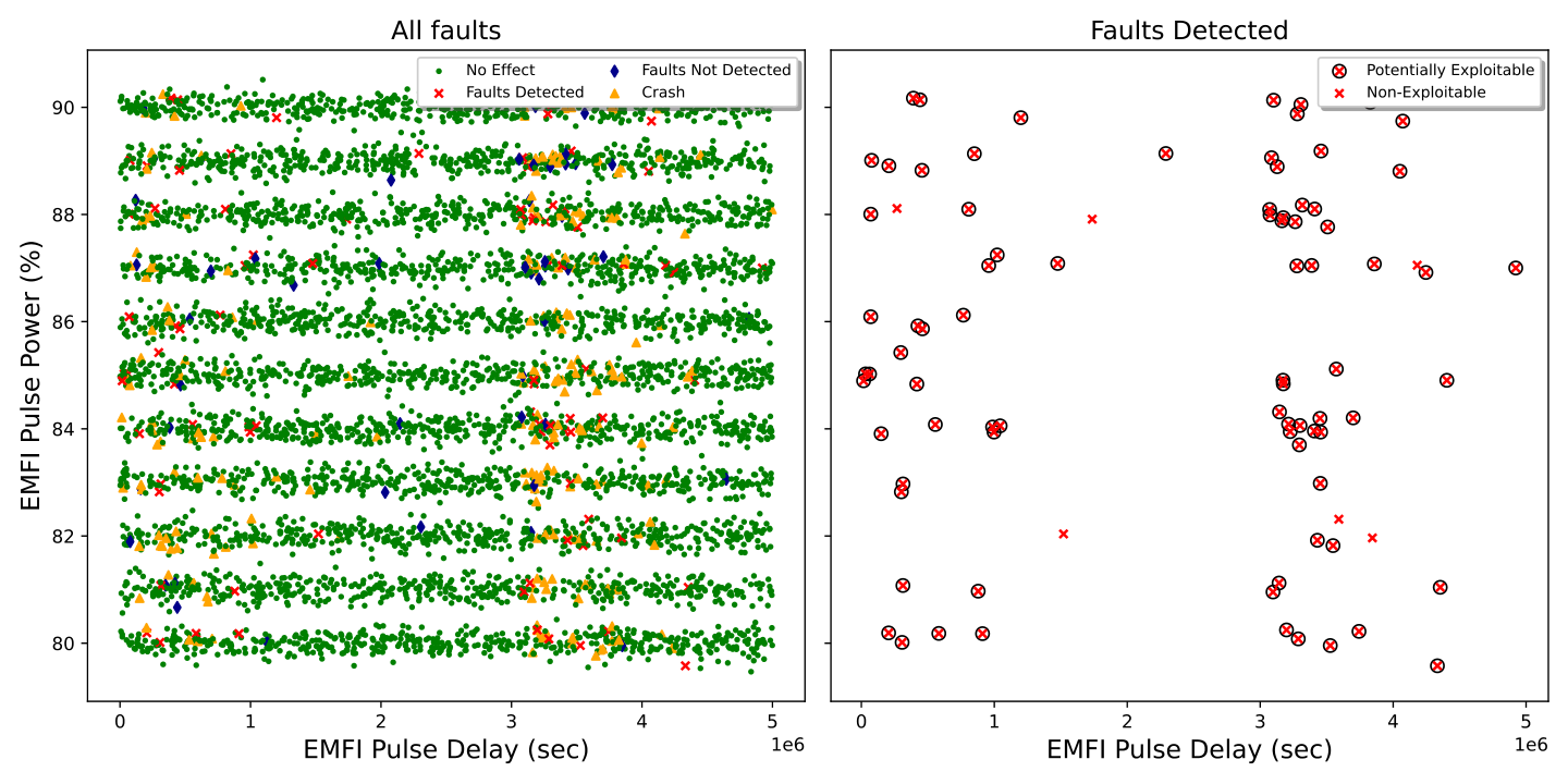
| Classification | Amount | Percentage (%) | Potentially Exploitable | Non-Exploitable |
|---|---|---|---|---|
| No Effect | 5635 | 93.9157 | 0 | 5635 |
| Crash | 229 | 3.81667 | 0 | 229 |
| Faults Not Detected | 49 | 0.816667 | 46 | 3 |
| Faults Detected | 87 | 1.45 | 81 | 6 |
6.5.3. Experiment 3: Parametric-sweep of EMFI Pulse Power and EMFI Pulse Delay with a fixed x-y probe position
In this experiment, we perform parameter sweep between the narrowed-down ranges identified through Experiment 6.5.2. Using the parameters given in Table 9, we perform 3 measurements per step that leads to total 4824 measurements completed in 16 hours. The results of this experiment are shown in the Figure 12 and Table 10 further shows the distribution of fault response.
It is observed that the number of potentially exploitable faults has increased from 127 in Experiment 6.5.2 to 382 in this experiment. This result further confirms that the spatial parameter search process led to a precise location on the chip where we are able to achieve large number of attacker usable faults. The plot shows the same observation as in previous experiments that the attacker usable faults occur at similar locations or locations closer to crashes. In conclusion, our approach to injection parameters exploration is able to find reliable and highly repeatable potentially exploitable faults which affect the datapath are 61.7% while the remaining are control flow faults or memory faults.
| Injection Parameter | Value |
|---|---|
| x-y Probe Position | Fixed at (214638, 199832) |
| EMFI Pulse Delay | Sweep between 3M ns and 3.8M ns by steps of 4000 ns |
| EMFI Pulse Power | Sweep between 83% and 90% by steps of 1% |

| Classification | Amount | Percentage (%) | Potentially Exploitable | Non-Exploitable |
|---|---|---|---|---|
| No Effect | 3762 | 77.9851 | 0 | 3762 |
| Crash | 583 | 12.0854 | 0 | 583 |
| Faults Not Detected | 230 | 4.76783 | 146 | 84 |
| Faults Detected | 249 | 5.16169 | 236 | 13 |
7. Conclusion
We conclude that hardening the polynomial multiplication operations in Dilithium with the proposed countermeasure significantly reduced the probability of a successful fault injection attack and increased the time required to gain enough faulty signatures to mount a complete attack at the cost of increased computational complexity. FI attack surface for Dilithium is so large that any part of code may become a potential FI attack vector. Our countermeasure reduces the attack surface by protecting polynomial multiplication operations, second largest contributor to the run-time of the algorithm after hash operations. The proposed countermeasure estimates the percentage of potentially exploitable faults which affect the datapath as 62%. However, some exploitable faults are not detected because time redundancy is not implemented in the proposed countermeasure to detect control flow faults. Further, characterization of fault effects is required to better understand the behavior of undetected potentially exploitable faults at software level. We plan to extend our bit-sliced NTT design with temporal IIR to detect faults in the control flow. Also, we intend to investigate the fault attack resistance of other finalist lattice-based schemes with our generic countermeasure.
References
- (1)
- Aysu et al. (2018) Aydin Aysu, Youssef Tobah, Mohit Tiwari, Andreas Gerstlauer, and Michael Orshansky. 2018. Horizontal side-channel vulnerabilities of post-quantum key exchange protocols. In 2018 IEEE International Symposium on Hardware Oriented Security and Trust (HOST). 81–88. https://doi.org/10.1109/HST.2018.8383894
- Banerjee et al. (2019) Utsav Banerjee, Tenzin S. Ukyab, and Anantha P. Chandrakasan. 2019. Sapphire: A Configurable Crypto-Processor for Post-Quantum Lattice-based Protocols. IACR Transactions on Cryptographic Hardware and Embedded Systems 2019, 4 (Aug. 2019), 17–61. https://doi.org/10.13154/tches.v2019.i4.17-61
- Bar-El et al. (2006) H. Bar-El, H. Choukri, D. Naccache, M. Tunstall, and C. Whelan. 2006. The Sorcerer’s Apprentice Guide to Fault Attacks. Proc. IEEE 94, 2 (2006), 370–382. https://doi.org/10.1109/JPROC.2005.862424
- Barenghi et al. (2010) Alessandro Barenghi, Luca Breveglieri, Israel Koren, Gerardo Pelosi, and Francesco Regazzoni. 2010. Countermeasures against Fault Attacks on Software Implemented AES: Effectiveness and Cost. In Proceedings of the 5th Workshop on Embedded Systems Security (Scottsdale, Arizona) (WESS ’10). Association for Computing Machinery, New York, NY, USA, Article 7, 10 pages. https://doi.org/10.1145/1873548.1873555
- Barrett (1986) Paul Barrett. 1986. Implementing the Rivest Shamir and Adleman Public Key Encryption Algorithm on a Standard Digital Signal Processor. In Advances in Cryptology - CRYPTO ’86, Santa Barbara, California, USA, 1986, Proceedings (Lecture Notes in Computer Science, Vol. 263). Springer, 311–323. https://doi.org/10.1007/3-540-47721-7_24
- Belaïd et al. (2020) Sonia Belaïd, Pierre-Évariste Dagand, Darius Mercadier, Matthieu Rivain, and Raphaël Wintersdorff. 2020. Tornado: Automatic Generation of Probing-Secure Masked Bitsliced Implementations. In Advances in Cryptology - EUROCRYPT 2020 - 39th Annual International Conference on the Theory and Applications of Cryptographic Techniques, Zagreb, Croatia, May 10-14, 2020, Proceedings, Part III (Lecture Notes in Computer Science, Vol. 12107), Anne Canteaut and Yuval Ishai (Eds.). Springer, 311–341. https://doi.org/10.1007/978-3-030-45727-3_11
- Biham (1997) Eli Biham. 1997. A Fast New DES Implementation in Software. In Fast Software Encryption, 4th International Workshop, FSE ’97, Haifa, Israel, January 20-22, 1997, Proceedings (Lecture Notes in Computer Science, Vol. 1267), Eli Biham (Ed.). Springer, 260–272. https://doi.org/10.1007/BFb0052352
- Bindel et al. (2016) Nina Bindel, Johannes Buchmann, and Juliane Krämer. 2016. Lattice-Based Signature Schemes and their Sensitivity to Fault Attacks. In FDTC 2016 - Fault Diagnosis and Tolerance in Cryptography. IEEE Conference Publication. http://tubiblio.ulb.tu-darmstadt.de/104111/
- Breier et al. (2021) Jakub Breier, Xiaolu Hou, and Yang Liu. 2021. On Evaluating Fault Resilient Encoding Schemes in Software. IEEE Transactions on Dependable and Secure Computing 18, 3 (2021), 1065–1079. https://doi.org/10.1109/TDSC.2019.2897663
- Bruinderink and Pessl (2018) Leon Groot Bruinderink and Peter Pessl. 2018. Differential fault attacks on deterministic lattice signatures. IACR Transactions on Cryptographic Hardware and Embedded Systems (2018), 21–43.
- Chen et al. (2021) Zhaohui Chen, Emre Karabulut, Aydin Aysu, Yuan Ma, and Jiwu Jing. 2021. An Efficient Non-Profiled Side-Channel Attack on the CRYSTALS-Dilithium Post-Quantum Signature. In 2021 IEEE 39th International Conference on Computer Design (ICCD). 583–590. https://doi.org/10.1109/ICCD53106.2021.00094
- Ciet and Joye (2005) Mathieu Ciet and Marc Joye. 2005. Practical Fault Countermeasures for Chinese Remaindering Based RSA ( Extended Abstract ).
- Cui and Housley (2017) Ang Cui and Rick Housley. 2017. BADFET: Defeating Modern Secure Boot Using Second-Order Pulsed Electromagnetic Fault Injection. In 11th USENIX Workshop on Offensive Technologies (WOOT 17). USENIX Association, Vancouver, BC. https://www.usenix.org/conference/woot17/workshop-program/presentation/cui
- Dehbaoui et al. (2012) Amine Dehbaoui, Jean-Max Dutertre, Bruno Robisson, and Assia Tria. 2012. Electromagnetic Transient Faults Injection on a Hardware and a Software Implementations of AES. In 2012 Workshop on Fault Diagnosis and Tolerance in Cryptography. 7–15. https://doi.org/10.1109/FDTC.2012.15
- Ducas et al. (2018) Léo Ducas, Eike Kiltz, Tancrede Lepoint, Vadim Lyubashevsky, Peter Schwabe, Gregor Seiler, and Damien Stehlé. 2018. Crystals-dilithium: A lattice-based digital signature scheme. IACR Transactions on Cryptographic Hardware and Embedded Systems (2018), 238–268.
- Elmohr et al. (2020) Mahmoud A. Elmohr, Haohao Liao, and Catherine H. Gebotys. 2020. EM Fault Injection on ARM and RISC-V. In 2020 21st International Symposium on Quality Electronic Design (ISQED). 206–212. https://doi.org/10.1109/ISQED48828.2020.9137051
- Espitau et al. (2017a) Thomas Espitau, Pierre-Alain Fouque, Benoît Gérard, and Mehdi Tibouchi. 2017a. Loop-Abort Faults on Lattice-Based Fiat-Shamir and Hash-and-Sign Signatures. In Selected Areas in Cryptography – SAC 2016, Roberto Avanzi and Howard Heys (Eds.). Springer International Publishing, Cham, 140–158.
- Espitau et al. (2017b) Thomas Espitau, Pierre-Alain Fouque, Benoît Gérard, and Mehdi Tibouchi. 2017b. Side-Channel Attacks on BLISS Lattice-Based Signatures. In 2017 ACM Conference on Computer and Communications Security (CCS 2017). ACM, Dallas, TX, United States, 1857–1874. https://doi.org/10.1145/3133956.3134028
- Facon et al. (2018) Adrien Facon, Sylvain Guilley, Matthieu Lec’Hvien, Alexander Schaub, and Youssef Souissi. 2018. Detecting Cache-Timing Vulnerabilities in Post-Quantum Cryptography Algorithms. In 2018 IEEE 3rd International Verification and Security Workshop (IVSW). 7–12. https://doi.org/10.1109/IVSW.2018.8494855
- Gaine et al. (2020) Clément Gaine, Driss Aboulkassimi, Simon Pontié, Jean-Pierre Nikolovski, and Jean-Max Dutertre. 2020. Electromagnetic Fault Injection as a New Forensic Approach for SoCs. In 2020 IEEE International Workshop on Information Forensics and Security (WIFS). 1–6. https://doi.org/10.1109/WIFS49906.2020.9360902
- Groot Bruinderink et al. (2016) L. Groot Bruinderink, A.T. Hülsing, T. Lange, and Y. Yarom. 2016. Flush, Gauss, and reload : a cache attack on the BLISS lattice-based signature scheme. IACR.
- Gruss et al. (2016) Daniel Gruss, Clémentine Maurice, and Stefan Mangard. 2016. Rowhammer. js: A remote software-induced fault attack in javascript. In International conference on detection of intrusions and malware, and vulnerability assessment. Springer, 300–321.
- Islam et al. (2022) Saad Islam, Koksal Mus, Richa Singh, Patrick Schaumont, and Berk Sunar. 2022. Signature Correction Attack on Dilithium Signature Scheme. CoRR abs/2203.00637 (2022). https://doi.org/10.48550/arXiv.2203.00637 arXiv:2203.00637
- Kiaei et al. (2021) Pantea Kiaei, Darius Mercadier, Pierre-Evariste Dagand, Karine Heydemann, and Patrick Schaumont. 2021. Custom Instruction Support for Modular Defense Against Side-Channel and Fault Attacks. In Constructive Side-Channel Analysis and Secure Design, Guido Marco Bertoni and Francesco Regazzoni (Eds.). Springer International Publishing, Cham, 221–253.
- Kiaei and Schaumont (2021) Pantea Kiaei and Patrick Schaumont. 2021. Synthesis of Parallel Synchronous Software. IEEE Embedded Systems Letters 13, 1 (2021), 17–20. https://doi.org/10.1109/LES.2020.2992051
- Majéric et al. (2016) F. Majéric, E. Bourbao, and L. Bossuet. 2016. Electromagnetic security tests for SoC. In 2016 IEEE International Conference on Electronics, Circuits and Systems (ICECS). 265–268. https://doi.org/10.1109/ICECS.2016.7841183
- Menu et al. (2019) Alexandre Menu, Shivam Bhasin, Jean-Max Dutertre, Jean-Baptiste Rigaud, and Jean-Luc Danger. 2019. Precise Spatio-Temporal Electromagnetic Fault Injections on Data Transfers. In 2019 Workshop on Fault Diagnosis and Tolerance in Cryptography (FDTC). 1–8. https://doi.org/10.1109/FDTC.2019.00009
- Moody et al. (2020) Dustin Moody, Gorjan Alagic, Daniel Apon, David Cooper, Quynh Dang, John Kelsey, Yi-Kai Liu, Carl Miller, Rene Peralta, Ray Perlner, Angela Robinson, Daniel Smith-Tone, and Jacob Alperin-Sheriff. 2020. Status Report on the Second Round of the NIST Post-Quantum Cryptography Standardization Process. https://doi.org/10.6028/NIST.IR.8309
- Moro et al. (2013) Nicolas Moro, Amine Dehbaoui, Karine Heydemann, Bruno Robisson, and Emmanuelle Encrenaz. 2013. Electromagnetic Fault Injection: Towards a Fault Model on a 32-bit Microcontroller. In 2013 Workshop on Fault Diagnosis and Tolerance in Cryptography. 77–88. https://doi.org/10.1109/FDTC.2013.9
- Patrick et al. (2016) Conor Patrick, Bilgiday Yuce, Nahid Farhady Ghalaty, and Patrick Schaumont. 2016. Lightweight Fault Attack Resistance in Software Using Intra-instruction Redundancy. In Selected Areas in Cryptography - SAC 2016 - 23rd International Conference, St. John’s, NL, Canada, August 10-12, 2016, Revised Selected Papers (Lecture Notes in Computer Science, Vol. 10532), Roberto Avanzi and Howard M. Heys (Eds.). Springer, 231–244. https://doi.org/10.1007/978-3-319-69453-5_13
- Pessl (2017) Peter Pessl. 2017. Analyzing the Shuffling Side-Channel Countermeasure for Lattice-Based Signatures. IACR Cryptol. ePrint Arch. (2017), 33. http://eprint.iacr.org/2017/033
- Pessl et al. (2017) Peter Pessl, Leon Groot Bruinderink, and Yuval Yarom. 2017. To BLISS-B or Not to Be: Attacking StrongSwan’s Implementation of Post-Quantum Signatures. In Proceedings of the 2017 ACM SIGSAC Conference on Computer and Communications Security (Dallas, Texas, USA) (CCS ’17). Association for Computing Machinery, New York, NY, USA, 1843–1855. https://doi.org/10.1145/3133956.3134023
- Pessl and Primas (2019) Peter Pessl and Robert Primas. 2019. More Practical Single-Trace Attacks on the Number Theoretic Transform. In Progress in Cryptology – LATINCRYPT 2019, Peter Schwabe and Nicolas Thériault (Eds.). Springer International Publishing, Cham, 130–149.
- Pessl and Prokop (2021) Peter Pessl and Lukas Prokop. 2021. Fault Attacks on CCA-secure Lattice KEMs. IACR Trans. Cryptogr. Hardw. Embed. Syst. 2021, 2 (2021), 37–60. https://doi.org/10.46586/tches.v2021.i2.37-60
- Primas et al. (2017) Robert Primas, Peter Pessl, and Stefan Mangard. 2017. Single-Trace Side-Channel Attacks on Masked Lattice-Based Encryption. In Cryptographic Hardware and Embedded Systems – CHES 2017, Wieland Fischer and Naofumi Homma (Eds.). Springer International Publishing, Cham, 513–533.
- Proy et al. (2019) Julien Proy, Karine Heydemann, Fabien Majéric, Albert Cohen, and Alexandre Berzati. 2019. Studying EM Pulse Effects on Superscalar Microarchitectures at ISA Level. https://doi.org/10.48550/ARXIV.1903.02623
- Ravi et al. (2018) Prasanna Ravi, Mahabir Prasad Jhanwar, James Howe, Anupam Chattopadhyay, and Shivam Bhasin. 2018. Side-channel Assisted Existential Forgery Attack on Dilithium-A NIST PQC candidate. IACR Cryptol. ePrint Arch. 2018 (2018), 821.
- Ravi et al. (2019a) Prasanna Ravi, Mahabir Prasad Jhanwar, James Howe, Anupam Chattopadhyay, and Shivam Bhasin. 2019a. Exploiting determinism in lattice-based signatures: practical fault attacks on pqm4 implementations of NIST candidates. In Proceedings of the 2019 ACM Asia Conference on Computer and Communications Security. 427–440.
- Ravi et al. (2020) Prasanna Ravi, Romain Poussier, Shivam Bhasin, and Anupam Chattopadhyay. 2020. On Configurable SCA Countermeasures Against Single Trace Attacks for the NTT: A Performance Evaluation Study over Kyber and Dilithium on the ARM Cortex-M4. In Security, Privacy, and Applied Cryptography Engineering: 10th International Conference, SPACE 2020, Kolkata, India, December 17–21, 2020, Proceedings. Springer-Verlag, Berlin, Heidelberg, 123–146. https://doi.org/10.1007/978-3-030-66626-2_7
- Ravi et al. (2019b) Prasanna Ravi, Debapriya Basu Roy, Shivam Bhasin, Anupam Chattopadhyay, and Debdeep Mukhopadhyay. 2019b. Number “not used” once-practical fault attack on pqm4 implementations of NIST candidates. In International Workshop on Constructive Side-Channel Analysis and Secure Design. Springer, 232–250.
- Riscure (2001) Riscure. 2001. Inspector FI. Retrieved March 25, 2022 from https://www.riscure.com/security-tools/inspector-fi
- Rivière et al. (2015) Lionel Rivière, Zakaria Najm, Pablo Rauzy, Jean-Luc Danger, Julien Bringer, and Laurent Sauvage. 2015. High precision fault injections on the instruction cache of ARMv7-M architectures. In 2015 IEEE International Symposium on Hardware Oriented Security and Trust (HOST). 62–67. https://doi.org/10.1109/HST.2015.7140238
- Schmidt and Hutter (2007) Jörn-Marc Schmidt and Michael Hutter. 2007. Optical and EM Fault-Attacks on CRT-based RSA: Concrete Results. In Austrochip 2007, 15th Austrian Workhop on Microelectronics, 11 October 2007, Graz, Austria, Proceedings. Verlag der Technischen Universität Graz, 61–67. Austrochip 2007 ; Conference date: 11-10-2007 Through 11-10-2007.
- Schmidt and Medwed (2012) Jörn-Marc Schmidt and Marcel Medwed. 2012. Countermeasures for Symmetric Key Ciphers (1 ed.). Springer, 73–88.
- Shor (1994) Peter W. Shor. 1994. Polynomial time algorithms for discrete logarithms and factoring on a quantum computer. In Algorithmic Number Theory, Leonard M. Adleman and Ming-Deh Huang (Eds.). Springer Berlin Heidelberg, Berlin, Heidelberg, 289–289.
- Trouchkine et al. (2019) Thomas Trouchkine, Sébanjila Kevin Bukasa, Mathieu Escouteloup, Ronan Lashermes, and Guillaume Bouffard. 2019. Electromagnetic fault injection against a System-on-Chip, toward new micro-architectural fault models. CoRR abs/1910.11566 (2019). arXiv:1910.11566 http://arxiv.org/abs/1910.11566
- Valencia et al. (2018) Felipe Valencia, Tobias Oder, Tim Güneysu, and Francesco Regazzoni. 2018. Exploring the Vulnerability of R-LWE Encryption to Fault Attacks. In Proceedings of the Fifth Workshop on Cryptography and Security in Computing Systems (Manchester, United Kingdom) (CS2 ’18). Association for Computing Machinery, New York, NY, USA, 7–12. https://doi.org/10.1145/3178291.3178294
- Wolf (2012) Clifford Wolf. 2012. Yosys Open Synthesis Suite. https://yosyshq.net/yosys/.
- Xagawa et al. (2021) Keita Xagawa, Akira Ito, Rei Ueno, Junko Takahashi, and Naofumi Homma. 2021. Fault-Injection Attacks against NIST’s Post-Quantum Cryptography Round 3 KEM Candidates. Springer-Verlag. https://doi.org/10.1007/978-3-030-92075-3_2
- Xu et al. (2021) Zhuang Xu, Owen Pemberton, Sujoy Sinha Roy, David Oswald, Wang Yao, and Zhiming Zheng. 2021. Magnifying Side-Channel Leakage of Lattice-Based Cryptosystems with Chosen Ciphertexts: The Case Study of Kyber. IEEE Trans. Comput. (27 Oct. 2021). https://doi.org/10.1109/TC.2021.3122997