跳到论文正文
W Papers独立论文阅读器 arXiv:2204.06104 论文正文 计算阅读时间 · 0%
引用这篇论文根据当前论文元数据生成,正式投稿前建议核对。


License: CC BY-NC-ND 4.0
arXiv:2204.06104v3 [eess.SY] 24 Apr 2022

A Tutorial on Solution Properties of State Space Models of Dynamical Systems

Bassam Bamieh Thanks: Department of Mechanical Engineering, University of California at Santa Barbara, bamieh@ucsb.edu. This work is partially supported by NSF Awards CMMI-1763064 and ECCS-1932777.
Abstract

The starting point of analysis of state space models is investigating existence, uniqueness and solution properties such as the semigroup property, and various formulas for the solutions. Several concepts such as the state transition matrix, the matrix exponential, the variations of constants formula (the Cauchy formula), the Peano-Baker series, and the Picard iteration are used to characterize solutions. In this note, a tutorial treatment is given where all of these concepts are shown to be various manifestations of a single abstract method, namely solving equations using an operator Neumann series involving the Volterra operator of forward integration. The matrix exponential, the Peano-Baker series, the Picard iteration, and the Cauchy formula can be “discovered” naturally from this Neumann series. The convergence of the series and iterations is a consequence of the key property of asymptotic nilpotence of the Volterra operator. This property is an asymptotic version of the nilpotence property of a strictly-lower-triangular matrix.

1 Introduction

State space models are the starting point in analysis of dynamical systems. They come in various forms of generality as follows

(a):x˙​(t)\displaystyle(a):~\dot{x}(t) =A(x(t),t),\displaystyle=~A\big(x(t),t\big),\hskip 20.00003pt\hskip 20.00003pt (b):x˙​(t)\displaystyle(b):~\dot{x}(t) =A⁡(x⁡(t),u⁡(t)),\displaystyle=~A\big(x(t),u(t)\big), (1)
(c):x˙​(t)\displaystyle(c):~\dot{x}(t) =A⁡(t)​x​(t),\displaystyle=~A(t)~x(t), (d):x˙​(t)\displaystyle(d):~\dot{x}(t) =A⁡(t)​x​(t)+B⁡(t)​u​(t),\displaystyle=~A(t)~x(t)~+~B(t)~u(t),
(e):x˙​(t)\displaystyle(e):~\dot{x}(t) =A​x​(t),\displaystyle=~A~x(t), (f):x˙​(t)\displaystyle(f):~\dot{x}(t) =A​x​(t)+B​u​(t).\displaystyle=~A~x(t)~+~B~u(t).

The state at each time x⁡(t)∈ℝnx(t)\in{\mathbb{R}}^{n} is an nn-vector, while the input u⁡(t)∈ℝqu(t)\in{\mathbb{R}}^{q} is also a vector at each tt, with typically a different dimension than the state. For control problems, for example, the signal uu is the control input, and most interesting problems have the dimension of uu being much less than that of xx (controlling many states with a single or few inputs). If the signal uu is a disturbance or a noise signal, it typically has dimensions comparable to those of the state xx.

The first column in (1) represents systems without an external input, and we generally want to understand their responses {x⁡(t)}\left\{x(t)\right\} due to various boundary conditions x⁡(t¯)x({\bar{t}}) specified at some time t¯{\bar{t}}. In the second column, the signal uu is regarded as an external signal, and we typically want to establish response properties for a whole class of inputs uu rather than a single, fixed input.

The systems in the first row are generally nonlinear, and without making more restrictive assumptions on the structure of the vector field AA, one can only deduce rather basic properties of existence and uniqueness of solutions. An important special instance of (a) is the time-invariant case where AA is constant in tt. The second row consists of linear time-varying systems. We will be able to say more about them, but in general these are capable of very rich behavior, and again without additional restrictive assumptions, only basic properties can be established. The third row represents linear time-invariant systems, and much more can be said about properties of those systems. Those statements will generally involve linear-algebraic properties of the matrices AA and BB. As a side note, when the state dimension becomes very large or infinite, the distinctions between the three categories of systems listed above can become quite blurry and in some cases cease to be relevant.

This tutorial is motivated by and organized around a pedagogical principle that it is better to discover results starting from basic, generally applicable principles than to simply be told what the answer is, and then just verify it. I will try to illustrate what I mean by this using the most concrete case of linear time-invariant systems. The traditional treatment [1, 2, 3] to derive formulas for the solution of a linear time-invariant state space system

x˙​(t)=A​x​(t)+w⁡(t),x⁡(0)=x¯\dot{x}(t)~=~Ax(t)~+~w(t),\hskip 20.00003pt\hskip 20.00003ptx(0)={\bar{x}} (2)

proceeds as follows. First, the homogenous problem with w⁡(t)=0w(t)=0 is addressed. The solution of this problem is given in terms of the matrix exponential. Given any square matrix AA, the exponential function is defined by the series formula

eA​t:=∑k=0∞Ak​tkk!=I+A​t+12​A2​t2+13!​A3​t3+⋯e^{At}~:=~\sum_{k=0}^{\infty}\frac{A^{k}t^{k}}{k!}~=~I+At+\frac{1}{2}A^{2}t^{2}+\frac{1}{3!}A^{3}t^{3}~+~\cdots

It is not difficult to show that this series is absolutely convergent for any matrix AA and time tt. Note also that e0=Ie^{0}=I. By differentiating this series element by element, it then follows that the derivative of this matrix-valued function is the matrix-valued function

dd​t​eA​t=A​eA​t=eA​t​A.\frac{d}{dt}e^{At}~=~A~e^{At}~=~e^{At}~A.

It is then an easy verification that the solution of (2) (with w=0w=0) is given by

x⁡(t)=eA​t​x¯,since\displaystyle x(t)~=~e^{At}{\bar{x}},\hskip 20.00003pt\hskip 20.00003pt\mbox{since} x˙​(t)=dd​t​eA​t​x¯=A​eA​t​x¯=A​x​(t),\displaystyle\dot{x}(t)~=~\frac{d}{dt}e^{At}{\bar{x}}~=~A~e^{At}{\bar{x}}~=~A~x(t), (3)
and\displaystyle~\mbox{and} x⁡(0)=eA​t​x¯|t=0=e0​x¯=I​x¯=x¯.\displaystyle\left.x(0)~=~e^{At}{\bar{x}}\right|_{t=0}~=~e^{0}{\bar{x}}~=~I{\bar{x}}~=~{\bar{x}}.

The solution of (2) with a non-zero forcing function ww is given by the ‘‘variations-of-constants’’ formula11 1 This is also known as the Cauchy formula.

x⁡(t)=eA​t​x¯+∫0t​eA⁡(t−τ)​w​(τ)​d​τ.x(t)~=~e^{At}{\bar{x}}~+~\mathchoice{\scalebox{.8}{$\displaystyle\int_{{0}}^{{t}}$}}{\scalebox{.8}{$\textstyle\int_{{0}}^{{t}}$}}{\scalebox{.8}{$\scriptstyle\int_{{0}}^{{t}}$}}{\scalebox{.8}{$\scriptscriptstyle\int_{{0}}^{{t}}$}}e^{A(t-\tau)}~w(\tau)~d\tau. (4)

The fact that this formula gives x⁡(t)x(t) that satisfies the differential equation (2) can be directly verified by differentiation.

The development described above, while quick and expedient, is unsatisfactory. Although it might be easy to guess the definition of the matrix exponential, and the solution (3) as a generalization of the well known scalar case, it is difficult to see how this might generalize to the linear time-varying or the nonlinear cases. Again, from a pedagogical point of view, being told what the answer to a problem is, and your role is simply to verify that it is indeed the answer is not helpful in gaining insight into how more general situations might be addressed. For example, if you have not seen the formula (4) before, it probably seems to “come out of thin air”. It is easy to verify, but where did it come from? What would a similar formula be in the time-varying case, or if the state xx is a matrix rather than a vector?

A more satisfactory development is to see the answer emerge naturally from basic, familiar principles that are applicable to a large variety of problem settings. At the expense of a little bit of abstraction, we can have a better, more contextual understanding of the subject. This is the approach we will follow in this paper which is organized around the following central idea. The differential equations (1) are rewritten as integral equations, which can then be thought of as equations in an abstract function space involving the Volterra operator of forward integration. This operator has very special properties which we investigate. The various series expressions and iterative algorithms for solutions follow from Neumann series involving this operator. In particular, the matrix exponential, the Peano-Baker series, the variations-of-constants formula, and the Picard iteration are all specific manifestations of this abstract Neumann series. They all emerge naturally from applying the Neumann series without having to guess the answer. Furthermore, the convergence properties of all these series and iterations follow from an asymptotic nilpotence property of the Volterra operator. This gives a unified view of all the various results in this area.

This presentation is organized as follows.

Section 2:

Introduces the basic properties of flow maps, and their special forms when the dynamics are time-invariant or linear respectively. These properties follow from the basic assumptions of existence and uniqueness.

Section 3:

Recasts the solution of state-space models in the linear case as a linear algebra problem in function space. The Volterra (forward) integration operator is introduced as analogous to strictly lower-triangular matrices. Such matrices are nilpotent, and the Volterra operator is shown to be “asymptotically nilpotent”. Convergence of series and iterations with the Voiterra operator then follow from this latter property. The kernel representation of linear operators is introduced here as the main tool to understand these properties.

Section 4:

Shows how the matrix exponential and the Peano-Baker series are special instances of the Neuman series.

Section 5:

Considers systems with inputs in the linear case. The well-known “variations-of-constants” (Cauchy) formula is derived in three different ways, one of which is again as a consequence of the Neumann series. Readers not interested in systems with inputs can skip this section.

Section 6:

Considers general non-linear systems. The Neumann series here becomes the Picard iteration. The proof of convergence follow from fixed point theorems. The standard contraction mapping theorem is used to show local existence and uniqueness. A tighter fixed point theorem that uses the asymptotic nilpotence of the Volterra operator is used to show global existence and uniqueness.

2 Basic Properties

We consider first systems without inputs (systems (a), (c) and (e) in (1)). We will give various conditions for existence and uniqueness of solutions later on in Section 6. For now however, we will make the following standing assumption.

Definition 1.

A system of the form (1) without input is said to be well posed over a time interval (a,b)⊆ℝ(a,b)\subseteq{\mathbb{R}} if for any initial time t¯∈(a,b){\bar{t}}\in(a,b), and any initial condition x⁡(t¯)∈ℝnx({\bar{t}})\in{\mathbb{R}}^{n}, there exists a unique solution of the differential equation over (a,b)(a,b). aa or bb may be −∞-\infty or ∞\infty respectively, and intervals can also be half open (i.e. [a,b)[a,b) or (a,b](a,b]).

It should be noted that a requirement of existence and uniqueness of solutions is a natural one when differential equations are used as mathematical models of physical phenomena. If solutions are non-unique, then the model must be missing some feature of the physical phenomenon, and likewise if solutions do not exist for some initial conditions. Further commentary along these lines is included in Section 6.4 after the conditions for existence and uniqueness are established.

2.1 The Flow Map

Consider now any of the systems (a), (c) and (e) in (1), and assume well-posedness over [0,T)[0,T) for some TT. The existence and uniqueness of solutions assumption implies that for each t,t¯∈[0,T)t,{\bar{t}}\in[0,T) there is a well-defined mapping Φt,t¯:ℝn→ℝn\Phi_{t,{\bar{t}}}:{\mathbb{R}}^{n}\rightarrow{\mathbb{R}}^{n} such that

x⁡(t)=Φt,t¯​(x⁡(t¯)).x(t)~=~\Phi_{t,{\bar{t}}}\big(x({\bar{t}})\big). (5)

We don’t know this mapping explicitly. This mapping is simply the statement that x⁡(t)x(t) is the solution of the differential equation at time tt given the initial condition x⁡(t¯)x({\bar{t}}) at time t¯{\bar{t}}. Since solutions exist and are unique by assumption, this is a well defined mapping. More precisely, Φ:={Φt,t¯,t,t¯∈[0,∞)}\Phi:=\left\{\Phi_{t,{\bar{t}}},~t,{\bar{t}}\in[0,\infty)\right\} is a two-parameter family of mappings on ℝn{\mathbb{R}}^{n}. We refer to Φ\Phi as the flow map of the dynamical system.

The flow map’s dependence on the parameters has properties that follow immediately from its definition. First, at any t∈[0,T)t\in[0,T)

Φt,t=I,\Phi_{t,t}~=~I,

where II is the identity map. This follows since Φt,t\Phi_{t,t} maps an initial condition at tt to the solution at tt, i.e. it maps each vector to itself. Second, consider three time instants t1,t2,t3∈[0,T)t_{1},t_{2},t_{3}\in[0,T). If we solve the equation from t1t_{1} to t3t_{3} starting from x⁡(t1)x(t_{1}), then the solution x⁡(t3)x(t_{3}) must be the same as what is obtained by solving the equation from t1t_{1} to t2t_{2} and then again from t2t_{2} to t3t_{3}, with the latter starting from x⁡(t2)x(t_{2}) as an initial condition (see Figure 1(a) for an illustration). In other words

x⁡(t3)=Φt3,t1​(x⁡(t1))=Φt3,t2​(x⁡(t2))=Φt3,t2​(Φt2,t1​(x⁡(t1))​)=(Φt3,t2∘Φt2,t1​)​(x⁡(t1)),x(t_{3})~=~\Phi_{t_{3},t_{1}}\big(x(t_{1})\big)~=~\Phi_{t_{3},t_{2}}\big(x(t_{2})\big)~=~\Phi_{t_{3},t_{2}}\left(\Phi_{t_{2},t_{1}}\big(x(t_{1})\big)\rule{0.0pt}{10.00002pt}\right)~=~\big(\Phi_{t_{3},t_{2}}\circ\Phi_{t_{2},t_{1}}\rule{0.0pt}{10.00002pt}\big)\big(x(t_{1})\big),

where the symbol ∘\circ denotes function composition. Since this has to hold for all possible initial conditions, we have equality of the mappings

Φt3,t1=Φt3,t2∘Φt2,t1\Phi_{t_{3},t_{1}}~=~\Phi_{t_{3},t_{2}}\circ\Phi_{t_{2},t_{1}} (6)

for all t1,t2,t3∈[0,T)t_{1},t_{2},t_{3}\in[0,T). This property is called the semigroup property, although this name is better suited for the time-invariant case which we discuss next.

(a) The semigroup property Φt3,t1=Φt3,t2∘Φt2,t1\Phi_{t_{3},t_{1}}=\Phi_{t_{3},t_{2}}\circ\Phi_{t_{2},t_{1}} is equivalent to saying that finding the solution at time t3t_{3} given an initial condition at time t1t_{1} is equivalent to solving in two steps. First, find the solution x⁡(t2)x(t_{2}) at some intermediate time t2t_{2} from the initial condition at t1t_{1}, then find the solution at time t3t_{3} from x⁡(t2)x(t_{2}) regarded as an initial condition at t2t_{2}. The answer should be the same as the going directly from t1t_{1} to t3t_{3}.
(b) The time invariance property implies that the solution x⁡(t)x(t) given an initial condition x⁡(t¯)x({\bar{t}}) is the same as solving a time-shifted problem (depicted in green), i.e. solving for xs​(t−t¯)x_{\rm s}(t-{\bar{t}}) from an initial condition xs​(0)=x​(t¯)x_{\rm s}(0)=x({\bar{t}}).
Figure 1: Well posed-ness (existence and uniqueness of solutions) of the system (1) implies that the solution x⁡(t2)x(t_{2}) at any time t2t_{2} from an initial conditions x⁡(t1)x(t_{1}) at time t1t_{1} is given by a well-defined, two-parameter family of mappings Φt2,t1:ℝn→ℝn\Phi_{t_{2},t_{1}}:{\mathbb{R}}^{n}\rightarrow{\mathbb{R}}^{n}. Well posedness also implies the semigroup property depicted in (a). When the system has constant (in time) coefficients, then the time-invariance (more precisely time-shift equivariance) property holds as depicted in (b), and the flow map is given by a single-parameter family Φt2,t1=Φt2​-​t1,0\Phi_{t_{2},t_{1}}=\Phi_{t_{2}\text{-}t_{1},0}.

2.2 Time Invariance

The concept of time invariance requires existence and uniqueness of solutions over semi-infinite time intervals. Without loss of generality, we will therefore assume well-posedness of the following system over the entire half line [0,∞)[0,\infty)

x˙​(t)=A⁡(x⁡(t)),t∈[0,∞),\dot{x}(t)~=~A\big(x(t)\big),\hskip 20.00003pt\hskip 20.00003ptt\in[0,\infty), (7)

where the vector field AA is constant in time. The “dynamics” of this system (i.e. the relation between x˙\dot{x} and xx at each time) are independent of tt. Suppose that x(.)x(.) is the solution from the initial condition x⁡(0)=x¯x(0)={\bar{x}}. Define the left-shift of xx by

xs​(t):=x⁡(t+t¯),t∈[0,∞),x_{\rm s}(t)~:=~x(t+{\bar{t}}),\hskip 20.00003pt\hskip 20.00003ptt\in[0,\infty),

where t¯{\bar{t}} is some fixed number. Note that the initial condition for xs​(0)x_{\rm s}(0) is x⁡(t¯)x({\bar{t}}). Now if we solve the equation from the initial condition xs​(0)=x​(t¯)x_{\rm s}(0)=x({\bar{t}}), the solution will simply be the portion of the original trajectory over [t¯,∞)[{\bar{t}},\infty), which is the same as xsx_{\rm s} over [0,∞)[0,\infty)

x˙s​(t)=x˙​(t+t¯)A​(xs​(t))=A⁡(x⁡(t+t¯))}⇒x˙​(t+t¯)=A⁡(x⁡(t+t¯))⇒{x˙s​(t)=A​(xs​(t))xs​(0)=x⁡(t¯).\left.\begin{array}[]{rcl}\dot{x}_{\rm s}(t)&=&\dot{x}(t+{\bar{t}})\\ A\big(x_{\rm s}(t)\big)&=&A\big(x(t+{\bar{t}})\big)\\ \end{array}\right\}\hskip 10.00002pt\Rightarrow\hskip 10.00002pt\dot{x}(t+{\bar{t}})=A\big(x(t+{\bar{t}})\big)\hskip 10.00002pt\Rightarrow\hskip 10.00002pt\left\{\begin{array}[]{rcl}\dot{x}_{\rm s}(t)&=&A\big(x_{\rm s}(t)\big)\\ x_{\rm s}(0)&=&x({\bar{t}})\\ \end{array}\right..

Thus the shifted function xsx_{\rm s} satisfies the differential equation with its initial condition as the vector x⁡(t¯)x({\bar{t}}). Figure 1(b) illustrates this property, which is called time invariance (or more precisely time-shift equivariance), for which we give a formal definition.

Definition 2.

Consider a state space system over [0,∞)[0,\infty). The system is called time invariant if for each solution trajectory {x⁡(t),t∈[0,∞)}\left\{x(t),~t\in[0,\infty)\right\}, and each t¯≥0{\bar{t}}\geq 0, the left-shifted trajectory xs​(t):=x⁡(t+t¯)x_{\rm s}(t):=x(t+{\bar{t}}) is a solution starting from the initial condition xs​(0)=x​(t¯)x_{\rm s}(0)=x({\bar{t}}).

The previous calculations show that a system of the form (7) where the vector field FF is independent of tt satisfies the definition above for time invariance. Note that the key to this fact is x˙​(t+t¯)=A⁡(x⁡(t+t¯))\dot{x}(t+{\bar{t}})=A\big(x(t+{\bar{t}})\big), which would not be true if the vector field AA depended on time since in general A⁡(x⁡(t+t¯),t+t¯)≠A⁡(x⁡(t+t¯),t)A\big(x(t+{\bar{t}}),t+{\bar{t}}\big)\neq A\big(x(t+{\bar{t}}),t\big).

Time invariance has an important implication for the dependence of the flow Φt2,t1\Phi_{t_{2},t_{1}} on the parameters t1t_{1} and t2t_{2}. Let xx be any trajectory, and let xs​(t):=x⁡(t+t1)x_{\rm s}(t):=x(t+t_{1}) be its shifted version. In terms of the flow maps, we have the relations

xs​(t):=x⁡(t+t1)\displaystyle x_{\rm s}(t)~:=~x(t+t_{1})\hskip 20.00003pt ⇒xs​(0)=x⁡(t1)​and​xs​(t2−t1)=x⁡(t2),\displaystyle\Rightarrow\hskip 20.00003ptx_{\rm s}(0)=x(t_{1})~\mbox{and}~x_{\rm s}(t_{2}-t_{1})=x(t_{2}),
x⁡(t2)=Φt2,t1​(x⁡(t1))xs​(t2−t1)=Φt2​-​t1,0​(xs​(0))=Φt2​-​t1,0​(x⁡(t1))}\displaystyle\left.\begin{array}[]{rcl}x(t_{2})&=&\Phi_{t_{2},t_{1}}\big(x(t_{1})\big)\\ x_{\rm s}(t_{2}-t_{1})&=&\Phi_{t_{2}\text{-}t_{1},0}\big(x_{\rm s}(0)\big)\\ &=&\Phi_{t_{2}\text{-}t_{1},0}\big(x(t_{1})\big)\end{array}\right\} ⇒Φt2,t1​(x⁡(t1))=Φt2​-​t1,0​(x⁡(t1))\displaystyle\Rightarrow\hskip 20.00003pt\Phi_{t_{2},t_{1}}\big(x(t_{1})\big)=\Phi_{t_{2}\text{-}t_{1},0}\big(x(t_{1})\big)

Since this last statement must hold for all possible vectors x⁡(t1)x(t_{1}), we conclude that as maps

Φt2,t1=Φt2​-​t1,0.\Phi_{t_{2},t_{1}}~=~\Phi_{t_{2}\text{-}t_{1},0}.

Thus the two-parameter family of flow maps is fully determined by the one parameter family {Φt,0,t∈[0,∞)}\left\{\Phi_{t,0},~t\in[0,\infty)\right\}. With a slight abuse of notation, we relabel this family as Φt\Phi_{t} and state this conclusion formally.

Lemma 3.

Assume the time-invariant dynamical system (7) is well posed over [0,∞)[0,\infty). Then there exists a one parameter family of maps Φt:ℝn→ℝn\Phi_{t}:{\mathbb{R}}^{n}\rightarrow{\mathbb{R}}^{n}, t∈[0,∞)t\in[0,\infty) such that for any trajectory, and any times t2≥t1≥0t_{2}\geq t_{1}\geq 0

x⁡(t2)=Φt2​-​t1​(x⁡(t1)).x(t_{2})~=~\Phi_{t_{2}\text{-}t_{1}}\big(x(t_{1})\big).

In particular, x⁡(t)=Φt​(x⁡(0))x(t)~=~\Phi_{t}\big(x(0)\big).

Thus for time-invariant systems, the flow map between the state at time t1t_{1} and the state at time t2t_{2} depends only on the time difference t2−t1t_{2}-t_{1}, and not on the starting or ending times t1t_{1} and t2t_{2}. Now recall the so-called semigroup property , which when combined with time invariance says

Φt3,t1=Φt3,t2∘Φt2,t1\displaystyle\Phi_{t_{3},t_{1}}=\Phi_{t_{3},t_{2}}\circ\Phi_{t_{2},t_{1}}\hskip 20.00003pt ⇒Φt3​-​t1,0=Φt3​-​t2,0∘Φt2​-​t1,0\displaystyle\Rightarrow\hskip 20.00003pt\Phi_{t_{3}\text{-}t_{1},0}=\Phi_{t_{3}\text{-}t_{2},0}\circ\Phi_{t_{2}\text{-}t_{1},0}
⇒Φt3​-​t1=Φt3​-​t2∘Φt2​-​t1,\displaystyle\Rightarrow\hskip 20.00003pt\Phi_{t_{3}\text{-}t_{1}}=\Phi_{t_{3}\text{-}t_{2}}\circ\Phi_{t_{2}\text{-}t_{1}},

where we repeated the abuse of notation in the last statement. If we now relabel t2−t1=:τ1t_{2}-t_{1}=:\tau_{1} and t3−t2=:τ2t_{3}-t_{2}=:\tau_{2}, then t3−t1=τ2+τ1t_{3}-t_{1}=\tau_{2}+\tau_{1} and we can finally state that for time-invariant systems, the one-parameter family of flow maps satisfies the property

Φτ2∘Φτ1=Φτ2+τ1,τ1,τ2∈[0,∞).\Phi_{\tau_{2}}\circ\Phi_{\tau_{1}}~=~\Phi_{\tau_{2}+\tau_{1}},\hskip 20.00003pt\hskip 20.00003pt\tau_{1},\tau_{2}\in[0,\infty). (8)

This can now be legitimately called the semigroup property. There is a one-to-one correspondence between the set [0,∞)[0,\infty) (which is a semigroup under addition) and the family of maps Φ:={Φt,t∈[0,∞)}\Phi:=\left\{\Phi_{t},~t\in[0,\infty)\right\}. The property (8) is a statement of semigroup isomorphism. Φ\Phi is a semigroup with the operation of function composition, which is isomorphic to [0,∞)[0,\infty), a semigroup under addition.

2.3 The State Transition Matrix

In the case of linear systems, the flow map Φt2,t1\Phi_{t_{2},t_{1}} can be shown to be a linear mapping on ℝn{\mathbb{R}}^{n}, and is therefore represented by a matrix-valued function Φ⁡(t2,t1)\Phi(t_{2},t_{1}) of two parameteres, which is naturally called the state transition matrix. The fact that the flow map is linear is easy to show without actually “solving” the equation as follows. Consider a linear time-varying system with no input, and two solutions corresponding to two initial conditions

x˙1​(t)\displaystyle\dot{x}_{1}(t)~ =A⁡(t)​x1​(t),x1​(t¯)=x¯1,\displaystyle=~A(t)~x_{1}(t),\hskip 20.00003pt\hskip 20.00003ptx_{1}({\bar{t}})~=~{\bar{x}}_{1},
x˙2​(t)\displaystyle\dot{x}_{2}(t)~ =A⁡(t)​x2​(t),x2​(t¯)=x¯2.\displaystyle=~A(t)~x_{2}(t),\hskip 20.00003pt\hskip 20.00003ptx_{2}({\bar{t}})~=~{\bar{x}}_{2}.

We can immediately verify that the solution due to a linear combination x⁡(t¯)=α​x¯1+β​x¯2x({\bar{t}})=\alpha{\bar{x}}_{1}+\beta{\bar{x}}_{2} of the initial conditions is the same linear combination x⁡(t)=α​x1​(t)+β​x2​(t)x(t)=\alpha x_{1}(t)+\beta x_{2}(t) of the individual solutions. Indeed

dd​t​(α​x1​(t)+β​x2​(t))\displaystyle\frac{d}{dt}\big(\alpha x_{1}(t)+\beta x_{2}(t)\big)~ =α​x˙1​(t)+β​x˙2​(t)=α​A​(t)​x1​(t)+β​A​(t)​x2​(t)\displaystyle=~\alpha~\dot{x}_{1}(t)+\beta~\dot{x}_{2}(t)~=~\alpha~A(t)~x_{1}(t)+\beta~A(t)~x_{2}(t)
=A⁡(t)​(α​x1​(t)+β​x2​(t))\displaystyle=~A(t)~\big(\alpha~x_{1}(t)+\beta~x_{2}(t)\big)

Thus x⁡(t)=α​x1​(t)+β​x2​(t)x(t)=\alpha x_{1}(t)+\beta x_{2}(t) satisfies the differential equation as well as the initial condition. Note that the only property used above is the linearity of differentiation and the linearity of the right hand side of the differential equation.

Recall that the flow map Φt,t¯\Phi_{t,{\bar{t}}} maps initial conditions at t¯{\bar{t}} to solutions at tt. Since we have established that this map is linear, and on ℝn{\mathbb{R}}^{n} general linear maps are represented by matrices, then there must exist a matrix-valued function of time Φ⁡(t,t¯)\Phi(t,{\bar{t}}) such that

x⁡(t)\displaystyle x(t)~ =Φt,t¯​(x​(t¯)),\displaystyle=~\Phi_{t,{\bar{t}}}\big(x({\bar{t}})\big), Φt¯,t¯\displaystyle\Phi_{{\bar{t}},{\bar{t}}}~ =I(the identity mapping)\displaystyle=~I\hskip 20.00003pt\mbox{(the identity mapping)}
⇒x⁡(t)\displaystyle\Rightarrow\hskip 20.00003ptx(t)~ =Φ⁡(t,t¯)​x​(t¯)\displaystyle=~\Phi(t,{\bar{t}})~x({\bar{t}}) Φ⁡(t¯,t¯)\displaystyle\Phi({\bar{t}},{\bar{t}})~ =I(the identity matrix)\displaystyle=~I\hskip 20.00003pt\mbox{(the identity matrix)} (9)

This matrix-valued function of two time parameters Φ(.,.)\Phi(.,.) is naturally called the state transition matrix. It inherits properties of the flow map when specialized to linear maps. For example, Φt,t\Phi_{t,t} is the identity mapping for any tt, and since this linear map is represented by the matrix Φ⁡(t,t)\Phi(t,t), this must be the identity matrix. The semigroup property is also inherited, and in this case composition of maps becomes matrix multiplication. We now state these properties formally.

Lemma 4.

Consider the linear time-varying system

x˙​(t)=A⁡(t)​x​(t),x⁡(t¯)=x¯,\dot{x}(t)~=~A(t)~x(t),\hskip 20.00003pt\hskip 20.00003ptx({\bar{t}})={\bar{x}}, (10)

and assume it is well posed over ℝ{\mathbb{R}}. Then there exists a matrix-valued function, called the state transition matrix Φ(.,.)\Phi(.,.), such that for any two times t1,t2∈ℝt_{1},t_{2}\in{\mathbb{R}}

x⁡(t2)=Φ⁡(t2,t1)​x​(t1).x(t_{2})~=~\Phi(t_{2},t_{1})~x(t_{1}). (11)

This state transition matrix has the semigroup property where for any t1,t2,t3∈ℝt_{1},t_{2},t_{3}\in{\mathbb{R}}

Φ⁡(t3,t1)=Φ⁡(t3,t2)​Φ​(t2,t1).\Phi(t_{3},t_{1})~=~\Phi(t_{3},t_{2})~\Phi(t_{2},t_{1}). (12)

In particular, it is always non-singular and inverses are given by Φ−1​(t2,t1)=Φ⁡(t1,t2).\Phi^{-1}(t_{2},t_{1})=\Phi(t_{1},t_{2}). Furthermore, it satisfies the matrix differential equation

dd​t​Φ​(t,t¯)=A⁡(t)​Φ​(t,t¯),Φ⁡(t¯,t¯)=I,for any​t¯∈ℝ.\frac{d}{dt}\Phi(t,{\bar{t}})~=~A(t)~\Phi(t,{\bar{t}}),\hskip 20.00003pt\hskip 20.00003pt\Phi({\bar{t}},{\bar{t}})~=~I,\hskip 20.00003pt\mbox{for any}~{\bar{t}}\in{\mathbb{R}}. (13)

In the last section, we will show that this system is well posed on ℝ{\mathbb{R}} under the reasonable assumption that the function A(.)A(.) is bounded on bounded intervals. Well-posedness over all of ℝ{\mathbb{R}} implies that the system can be solved forward or backwards in time from any t¯∈ℝ{\bar{t}}\in{\mathbb{R}}.

The invertibility of the state transition matrix follows from the semigroup property since we can always expresses the inverse as

Φ⁡(t1,t2)​Φ​(t2,t1)=Φ⁡(t1,t1)=I.\Phi(t_{1},t_{2})~\Phi(t_{2},t_{1})~=~\Phi(t_{1},t_{1})~=~I.

In other words, solving from an initial condition x⁡(t1)x(t_{1}) at time t1t_{1} to the response x⁡(t2)x(t_{2}) at time t2t_{2}, and then solving backwards from x⁡(t2)x(t_{2}) to the state at time t1t_{1} should given the original x⁡(t1)x(t_{1}). Finally, the differential equation (13) can be verified from the formula (9) together with the original differential equation (32)

x˙​(t)=A⁡(t)​x​(t)x⁡(t)=Φ⁡(t,t¯)​x​(t¯)}⇒dd​t​Φ​(t,t¯)​x​(t¯)=A⁡(t)​Φ​(t,t¯)​x​(t¯).\left.\begin{array}[]{rcl}\dot{x}(t)&=&A(t)~x(t)\\ x(t)&=&\Phi(t,{\bar{t}})~x({\bar{t}})\end{array}\right\}\hskip 20.00003pt\Rightarrow\hskip 20.00003pt\frac{d}{dt}\Phi(t,{\bar{t}})~x({\bar{t}})~=~A(t)~\Phi(t,{\bar{t}})~x({\bar{t}}).

Since the last equality holds for any initial condition vector x⁡(t¯)x({\bar{t}}), then the matrix equation (13) must hold.

Another new ingredient here over the nonlinear case is the differential equation (13) for the state transition matrix. We note that it is possible to derive an analogous equation for the nonlinear flow map Φ\Phi (see Exercise 1), but it is a partial differential equation, and not particularly useful for computations due to the “curse of dimensionality”.

It is important to keep in mind that Lemma 4 does not “solve” the system (32) in any concrete sense. It just states the properties of the solution. The “solution formula” (11) is simply an expression of the linearity of the problem. The semigroup property is a consequence of the uniqueness of solutions. The differential equation (13) for Φ\Phi is actually more complicated to solve than the original system when given a specific initial condition. The latter is a vector differential equation, while the former is a matrix differential equation. However, as we will now demonstrate, if we solve nn vector differential equations from properly chosen initial conditions, we can find the state transition matrix.

Let {vk}k=1n\left\{v_{k}\right\}_{k=1}^{n} be any basis of ℝn{\mathbb{R}}^{n}. Suppose that we numerically solve the nn, vector differential equations

x˙k(t)=A(t)xk(t),xk(t¯)=vk,k=1,…,n,\dot{x}_{k}(t)~=~A(t)~x_{k}(t),\hskip 20.00003pt\hskip 20.00003ptx_{k}({\bar{t}})~=~v_{k},\hskip 20.00003ptk=1,\ldots,n, (14)

each with vkv_{k} as its initial condition. Those nn solutions can be used to obtain the solution for other initial conditions. Expand any initial condition x⁡(t¯)=x¯x({\bar{t}})={\bar{x}} using the basis, and write this in matrix-vector form as

x¯=∑k=1nαkvk⇔[x¯]=[v1⋯vn​][α1:αn]=:Vα{\bar{x}}~=~\sum_{k=1}^{n}\alpha_{k}v_{k}\hskip 20.00003pt\Leftrightarrow\hskip 20.00003pt\begin{bmatrix}\\ {\bar{x}}\\ ~\end{bmatrix}~=~\left[\begin{array}[]{c:c:c}v_{1}\hfil\lx@intercol\vrule\lx@add@cssclass&\cdots\hfil\lx@intercol\vrule\lx@add@cssclass&v_{n}\rule{0.0pt}{18.00005pt}\\ \hfil\lx@intercol\vrule\lx@add@cssclass&\hfil\lx@intercol\vrule\lx@add@cssclass&\end{array}\right]\begin{bmatrix}\alpha_{1}\\ :\\ \alpha_{n}\end{bmatrix}~=:~V~\alpha

Since the mapping from x⁡(t¯)x({\bar{t}}) to x⁡(t)x(t) is linear, then

x(t)=∑k=1nαkxk(t)=[x1​(t)⋯xn​(t)​][α1:αn]=Φ(t,t¯)x¯=Φ(t,t¯)Vα.x(t)~=~\sum_{k=1}^{n}\alpha_{k}x_{k}(t)~=~\left[\begin{array}[]{c:c:c}x_{1}(t)\hfil\lx@intercol\vrule\lx@add@cssclass&\cdots\hfil\lx@intercol\vrule\lx@add@cssclass&x_{n}(t)\rule{0.0pt}{18.00005pt}\\ \hfil\lx@intercol\vrule\lx@add@cssclass&\hfil\lx@intercol\vrule\lx@add@cssclass&\end{array}\right]\begin{bmatrix}\alpha_{1}\\ :\\ \alpha_{n}\end{bmatrix}~=~\Phi(t,{\bar{t}})~{\bar{x}}~=~\Phi(t,{\bar{t}})~V~\alpha.

Since this must hold for every initial conditions (i.e. for every vector α\alpha of coefficients), then

Φ⁡(t,t¯)=[x1​(t)⋯xn​(t)​]​[v1⋯vn​]−1\Phi(t,{\bar{t}})~=~\left[\begin{array}[]{c:c:c}x_{1}(t)\hfil\lx@intercol\vrule\lx@add@cssclass&\cdots\hfil\lx@intercol\vrule\lx@add@cssclass&x_{n}(t)\rule{0.0pt}{18.00005pt}\\ \hfil\lx@intercol\vrule\lx@add@cssclass&\hfil\lx@intercol\vrule\lx@add@cssclass&\end{array}\right]\left[\begin{array}[]{c:c:c}v_{1}\hfil\lx@intercol\vrule\lx@add@cssclass&\cdots\hfil\lx@intercol\vrule\lx@add@cssclass&v_{n}\rule{0.0pt}{18.00005pt}\\ \hfil\lx@intercol\vrule\lx@add@cssclass&\hfil\lx@intercol\vrule\lx@add@cssclass&\end{array}\right]^{-1} (15)

In other words, given a state dimension of nn, if we choose a basis {vk}k=1n\left\{v_{k}\right\}_{k=1}^{n} and solve the nn vector differential equations (14), then the state transition matrix is obtained from those nn vector functions of time by (15). Note that this formula satisfies Φ⁡(t¯,t¯)=V​V−1=I\Phi({\bar{t}},{\bar{t}})=VV^{-1}=I as required. A particularly simple choice of basis is the canonical basis {ek}k=1n\left\{e_{k}\right\}_{k=1}^{n}. The matrix VV in this case is the identity, and according to (15) the state transition matrix would simply be made from the nn solutions {xk​(t)}k=1n\left\{x_{k}(t)\right\}_{k=1}^{n} as its columns.

3 A Linear Algebra Problem in Function Space

The key to the solution formulas for the system (2) is a slight abstraction where we think of the system as a linear algebra problem but in function space. From this point of view, it is at first just as easy to do the time-varying case, which is a system of the form

x˙​(t)=A⁡(t)​x​(t)+w⁡(t),x⁡(0)=x¯\dot{x}(t)~=~A(t)~x(t)~+~w(t),\hskip 20.00003pt\hskip 20.00003ptx(0)={\bar{x}} (16)

This equation is equivalent to an integral equation which we obtain by Integrating both sides of (16)

x⁡(t)−x⁡(0)=∫0t​A​(τ)​x​(τ)​d​τ+∫0t​w​(τ)​d​τ.x(t)~-~x(0)~=~\mathchoice{\scalebox{.8}{$\displaystyle\int_{{0}}^{{t}}$}}{\scalebox{.8}{$\textstyle\int_{{0}}^{{t}}$}}{\scalebox{.8}{$\scriptstyle\int_{{0}}^{{t}}$}}{\scalebox{.8}{$\scriptscriptstyle\int_{{0}}^{{t}}$}}A(\tau)~x(\tau)~d\tau~+~\mathchoice{\scalebox{.8}{$\displaystyle\int_{{0}}^{{t}}$}}{\scalebox{.8}{$\textstyle\int_{{0}}^{{t}}$}}{\scalebox{.8}{$\scriptstyle\int_{{0}}^{{t}}$}}{\scalebox{.8}{$\scriptscriptstyle\int_{{0}}^{{t}}$}}w(\tau)~d\tau. (17)

To express this equation as a linear algebra problem, fix a time horizon [0,T][0,T], and define the Volterra integration operator, which we denote by the symbol 𝒱{\cal V}

(𝒱​g)​(t):=∫0t​g​(τ)​d​τ.\big({\cal V}g\big)(t)~:=~\mathchoice{\scalebox{.8}{$\displaystyle\int_{{0}}^{{t}}$}}{\scalebox{.8}{$\textstyle\int_{{0}}^{{t}}$}}{\scalebox{.8}{$\scriptstyle\int_{{0}}^{{t}}$}}{\scalebox{.8}{$\scriptscriptstyle\int_{{0}}^{{t}}$}}g(\tau)~d\tau. (18)

This operator is well-defined on the function space 𝖫n1​[0,T]{\sf L}^{\!1}_{n}[0,T]. Define also the operator

(𝒜​g)​(t):=A​(t)​g​(t)\big(\mathcal{A}g\big)(t)~:=~A(t)~g(t)

of point-wise (in time) multiplication by A(.)A(.). Finally define the operator 𝔥:ℝn→𝖫n1​[0,T]\mathfrak{h}:{\mathbb{R}}^{n}\rightarrow{\sf L}^{\!1}_{n}[0,T], which takes vectors x¯∈ℝn{\bar{x}}\in{\mathbb{R}}^{n} to constant functions of time by

(𝔥​x¯)​(t):=𝔥⁡(t)​x¯,t∈[0,T],\big(\mathfrak{h}{\bar{x}}\big)(t)~:=~\mathfrak{h}(t)~{\bar{x}},\hskip 20.00003pt\hskip 20.00003ptt\in[0,T],

where 𝔥(.)\mathfrak{h}(.) is the unit step (Heaviside) function

𝔥⁡(t):={1t≥00t<0.\mathfrak{h}(t)~:=~\left\{\begin{array}[]{lcl}1&&t\geq 0\\ 0&&t<0\end{array}\right..

Note the slight abuse of notation where we use the same symbol to denote a function 𝔥(.)\mathfrak{h}(.) of time, as well as this operator.

With the above definitions, the integral equation (17) can now be written as the abstract equation

x=𝒱​𝒜​x+𝒱​w+𝔥​x¯,x~=~{\cal V}\mathcal{A}~x~+~{\cal V}~w~+~\mathfrak{h}~{\bar{x}},

where 𝒱​𝒜{\cal V}\mathcal{A} is the composition of the action of the operator 𝒜\mathcal{A} (first) with the operator 𝒱{\cal V} (second). Since ww and x¯{\bar{x}} are usually given, we rewrite this equation so as to solve for xx in terms of the given quantities by

(I−𝒱​𝒜)​x=𝒱​w+𝔥​x¯.\big(I-{\cal V}\mathcal{A}\big)~x~=~{\cal V}w+\mathfrak{h}{\bar{x}}. (19)

The right hand side (𝒱​w+𝔥​x¯)({\cal V}w+\mathfrak{h}{\bar{x}}) and xx are functions over [0,T][0,T], and (I−𝒱​𝒜)\big(I-{\cal V}\mathcal{A}\big) is a linear operator on such functions. If this operator is invertible, then the solution is

​x=(I−𝒱​𝒜)−1​(𝒱​w+𝔥​x¯).\boxed{~\rule{0.0pt}{10.00002pt}x~=~\big(I-{\cal V}\mathcal{A}\big)^{-1}\big({\cal V}w+\mathfrak{h}{\bar{x}}\big).~} (20)

Thus we need to understand the operator (I−𝒱​𝒜)−1\big(I-{\cal V}\mathcal{A}\big)^{-1} and its properties. The key is the familiar Neumann series

(I−𝒱​𝒜)−1=I+𝒱​𝒜+(𝒱​𝒜)2+(𝒱​𝒜)3+⋯=∑n=0∞(𝒱​𝒜)n.\textstyle\big(I-{\cal V}\mathcal{A}\big)^{-1}~=~I~+~{\cal V}\mathcal{A}~+~\big({\cal V}\mathcal{A}\big)^{2}~+~\big({\cal V}\mathcal{A}\big)^{3}~+~\cdots~=~\sum_{n=0}^{\infty}\big({\cal V}\mathcal{A}\big)^{n}. (21)

The Neumann series has an interpretation as an iterative algorithm generally known as a fixed point iteration. Denote the right hand side of (19) by gg. The solution in terms of the Neumann series is then

x=(I−𝒱​𝒜)−1​g\displaystyle\textstyle x~=~\big(I-{\cal V}\mathcal{A}\big)^{-1}~g~ =g+𝒱​𝒜​g+(𝒱​𝒜)2​g+(𝒱​𝒜)3​g+⋯\displaystyle=~g~+~{\cal V}\mathcal{A}~g~+~\big({\cal V}\mathcal{A}\big)^{2}~g~+~\big({\cal V}\mathcal{A}\big)^{3}~g~+~\cdots (22)
=g+(𝒱​𝒜​(g+𝒱​𝒜​(g+𝒱​𝒜​(g+⋯))))\displaystyle=~g~+~\left({\cal V}\mathcal{A}~\left(g~+~{\cal V}\mathcal{A}~\left(g~+~{\cal V}\mathcal{A}~\left(g~+~\cdots~\right)\right)\right)\right)

This infinite series can be rewritten as the iterative algorithm

x0\displaystyle x_{0} =g,\displaystyle=~g, (23)
xk+1\displaystyle x_{k+1} =g+𝒱​𝒜​xk.\displaystyle=~g~+~{\cal V}\mathcal{A}~x_{k}.

Thus xkx_{k} is the kk’th partial sum of the series (22). If this series converges, then the limit x:=limk→∞xk=limk→∞xk+1x:=\lim_{k\rightarrow\infty}x_{k}=\lim_{k\rightarrow\infty}x_{k+1} satisfies

x=g+𝒱𝒜x⇔(I−𝒱𝒜)x=g,x~=~g~+~{\cal V}\mathcal{A}~x\hskip 20.00003pt\Leftrightarrow\hskip 20.00003pt\big(I-{\cal V}\mathcal{A}\big)~x~=~g,

and thus the limit of the iteration (23) is indeed a solution of the original problem. We will study the convergence properties of this iteration, which also is applicable to nonlinear problems under certain conditions. For now, we consider only linear problems.

It turns out that the Volterra integration operator 𝒱{\cal V} has a special property that guarantees the convergence of the Neumann series (21) under very mild conditions. In addition, this formula will lead naturally to the matrix exponential when AA is constant, and to the so-called Peano-Baker series in the time-varying case. First, we need to establish some important properties of 𝒱{\cal V}.

The Volterra integration operator 𝒱{\cal V} is analogous to a strictly lower triangular matrix with entries of 11 below the diagonal. This analogy is important to understand properties of this operator, and it is best done using the so-called kernel representation of linear operators which we now describe.

3.1 The Kernel Representation of Linear Operators

Let AA be an n×nn\times n matrix with the i​jij’th entry denoted by Ai​jA_{ij}. A matrix represents a linear operator on vectors by the matrix vector product v=A​uv=Au

v=Au⇔vi=∑j=1nAi​juj.v~=~A~u\hskip 20.00003pt\Leftrightarrow\hskip 20.00003ptv_{i}~=~\sum_{j=1}^{n}A_{ij}u_{j}. (24)

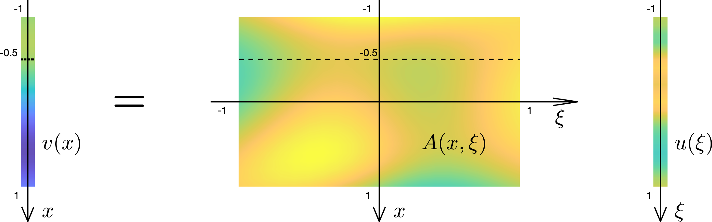
Now let 𝖨=(a,b)⊆ℝ{\sf I}=(a,b)\subseteq{\mathbb{R}} be any interval, and let A(.,.)A(.,.) be a real-valued function22 2 In the case when uu and vv are vector-valued functions, then A(.,.)A(.,.) would be a matrix-valued function. We suppress this distinction in our notation, which is equally applicable to either situation. of two variables from that interval A:𝖨×𝖨→ℝA:{\sf I}\times{\sf I}\rightarrow{\mathbb{R}}. Such a function defines a linear operator on single-variable functions over 𝖨{\sf I} in an analogous manner to (24) by

v=Au⇔v(x)=∫𝖨A(x,ξ)u(ξ)dξ,x∈𝖨,v~=~A~u\hskip 20.00003pt\Leftrightarrow\hskip 20.00003ptv(x)~=~\int_{{\sf I}}A(x,\xi)~u(\xi)~d\xi,\hskip 20.00003ptx\in{\sf I}, (25)

where the integration variable ξ\xi plays the same role as the column index jj over which the summation in (24) is performed. The operation in (25) is a linear operator A:u↦vA:u\mapsto v, and note the slight abuse of notation where we use the same symbol AA to denote the operator, as well as the function A(.,.)A(.,.) of two variables. The function A(.,.)A(.,.) is called the kernel function of the operator AA, and the formula (25) is called the kernel representation33 3 The reader should be careful not to confuse this with the null space of the operator, which is sometimes referred to as the kernel of the operator. The two concepts are unrelated. of AA.

Refer to caption
Figure 2: Graphical depiction of the integral operator (25) as an abstraction of matrix-vector multiplication. The two-variable kernel function A⁡(x,ξ)A(x,\xi) is the counterpart of matrix entries, with the coordinate xx as “row index” and ξ\xi as “column index”. The operation v⁡(x)=∫-​11A⁡(x,ξ)​u​(ξ)​𝑑ξv(x)=\int_{\text{-}1}^{1}A(x,\xi)~u(\xi)~d\xi gives the value of v⁡(x)v(x) at any xx (an instance above is depicted by the dashed lines at x=−0.5x=-0.5) as the multiply-then-integrate of the “xx’th row” of A(.,.)A(.,.) with the all the values of u⁡(ξ)u(\xi) viewed as a “column vector”. The case shown above is for an integral operator on functions defined over the interval [−1,1][-1,1]. The unusual choice of the vertical axis positive direction as downwards is made to be in analogy with matrix rows being indexed from top to bottom.

The operation (25) is depicted in Figure 2. The one-variable functions u⁡(ξ)u(\xi) and v⁡(x)v(x) are analogous to “column vectors”, while the two-variable kernel function A⁡(x,ξ)A(x,\xi) is analogous to a matrix, i.e. a two-dimensional array. For each xx, the value of v⁡(x)v(x) is given by the operation of multiply-then-integrate of the corresponding “row” of A⁡(x,ξ)A(x,\xi) with the function u⁡(ξ)u(\xi) in an analogous manner to matrix-vector multiplication.

Given two operators AA and BB in terms of their respective kernel functions, it is easy to see that the operator sum C:=A+BC:=A+B has as its kernel function C⁡(x,ξ)=A⁡(x,ξ)+B⁡(x,ξ)C(x,\xi)=A(x,\xi)+B(x,\xi)

v\displaystyle v =(A+B)​u=A​u+B​u\displaystyle=~\big(A+B\big)u~=~Au~+~Bu
v⁡(x)\displaystyle v(x) =∫A⁡(x,ξ)​u​(ξ)​𝑑ξ+∫B⁡(x,ξ)​u​(ξ)​𝑑ξ=∫(A⁡(x,ξ)+B⁡(x,ξ))​u​(ξ)​𝑑ξ.\displaystyle=~\int A(x,\xi)~u(\xi)~d\xi~+~\int B(x,\xi)~u(\xi)~d\xi~=~\int\big(A(x,\xi)+B(x,\xi)\big)~u(\xi)~d\xi.

Therefore, under addition, kernel functions behave just like matrix-matrix addition which is element-by-element.

Another intuitive property of kernel representations is that they can be composed in a manner similar to matrix-matrix multiplication. Let A:u↦vA:u\mapsto v and B:v↦wB:v\mapsto w be two operators with kernel representations

v⁡(x)=∫A⁡(x,ξ)​u​(ξ)​𝑑ξ,w⁡(x)=∫B⁡(x,ξ)​v​(ξ)​𝑑ξ.v(x)~=~\int A(x,\xi)~u(\xi)~d\xi,~~~~~~~~~~~~w(x)~=~\int B(x,\xi)~v(\xi)~d\xi.

Define a third operator as the composition C:=B​A:u↦wC:=BA:u\mapsto w, and calculate its kernel representation from those of AA and BB as follows

w⁡(x)=∫B⁡(x,ξ)​v​(ξ)​𝑑ξ\displaystyle w(x)=\int B(x,\xi)~v(\xi)~d\xi =∫B⁡(x,ξ)​(∫A⁡(ξ,r)​u​(r)​𝑑r)​𝑑ξ\displaystyle=\int B(x,\xi)\left(\int A(\xi,r)~u(r)~dr\right)~d\xi
=∫(∫B⁡(x,ξ)​A​(ξ,r)​𝑑ξ)​u​(r)​𝑑r=∫C⁡(x,r)​u​(r)​𝑑r.\displaystyle=\int\left(\int B(x,\xi)~A(\xi,r)~d\xi\right)~u(r)~dr=\int C(x,r)~u(r)~dr.

Thus the kernel of the composition C=B​AC=BA is obtained from the formula

Refer to caption
Figure 3: A graphical depiction of the composition of two operators C=B​AC=BA as the integral operation (26) on their respective kernels. This operation is akin to matrix-matrix multiplication as shown above. The value of the kernel CC at a point (x¯,r¯)(\bar{x},\bar{r}) is obtained from integrating the “row” B(x¯,.)B(\bar{x},.) against the “column” A(.,r¯)A(.,\bar{r}).
C⁡(x,r)=∫B⁡(x,ξ)​A​(ξ,r)​𝑑ξ,C(x,r)~=~\int B(x,\xi)~A(\xi,r)~d\xi, (26)

which looks like matrix-matrix multiplication except for integration instead of summation. Each “row” B(x,.)B(x,.) of the kernel of BB is integrated against each “column” A(.,r)A(.,r) of the kernel of AA. The composition operation (26) is depicted graphically in Figure 3. The reader should compare this visually with the usual matrix-matrix multiplication.

Lower-Triangular Operators

Just like certain matrix structures encode symmetries or properties of the linear operations they represent, the structure of a kernel encodes properties of the operators they represent. Figure 4(a) illustrates the structure of kernel functions of what can be termed “lower-triangular” operators. Such operators arise when modeling time-varying causal systems. The kernel is restricted to be zero in the “upper triangular part” of the (τ,t)(\tau,t) plane

A⁡(t,τ)=0,for​τ≥t.A(t,\tau)~=~0,~~~\mbox{for}~\tau\geq t. (27)

If uu and yy are temporal signals over the entire real line, then the lower-triangular property of the kernel implies that the integral (25) has the following limits

y⁡(t)=∫−∞∞A⁡(t,τ)​u​(τ)​𝑑τ=∫−∞tA⁡(t,τ)​u​(τ)​𝑑τ.y(t)~=~\int_{-\infty}^{\infty}A(t,\tau)~u(\tau)~d\tau~=~\int_{-\infty}^{t}A(t,\tau)~u(\tau)~d\tau. (28)

When tt and τ\tau are interpreted as time, then (28) is the description of a general time-varying system mapping uu to yy that has the causality property, i.e. for any given time tt, current and past values of the output {y⁡(τ);τ≤t}\left\{y(\tau);~\tau\leq t\right\} do not depend on future values of the input {u⁡(τ);τ>t}\left\{u(\tau);~\tau>t\right\}.

An alternative way of imposing the lower-triangular condition (27) is by using the unit-step (Heaviside) function 𝔥\mathfrak{h} as follows. Given any kernel function A⁡(x,ξ)A(x,\xi), observe that the product A⁡(x,ξ)​𝔥​(x−ξ)A(x,\xi)\mathfrak{h}\!\left(x-\xi\right) becomes a lower triangular kernel

∫ξ¯ξ¯(A⁡(x,ξ)​𝔥​(x−ξ))​u​(ξ)​𝑑ξ=∫ξ¯xA⁡(x,ξ)​u​(ξ)​𝑑ξ,\int^{\overline{\xi}}_{\underline{\xi}}\big(A(x,\xi)\mathfrak{h}\!\left(x-\xi\right)\big)~u(\xi)~d\xi~=~\int_{\underline{\xi}}^{x}A(x,\xi)~u(\xi)~d\xi,

since 𝔥⁡(x−ξ)=0\mathfrak{h}\!\left(x-\xi\right)=0 when ξ>x\xi>x. The above holds regardless of the original upper and lower integration limits ξ¯\overline{\xi} and ξ¯\underline{\xi} respectively.

Refer to caption
(a) A lower-triangular kernel is such that A⁡(t,τ)=0A(t,\tau)=0 for τ≥t\tau\geq t. If it operates on time signals, a lower-triangular kernel is a causal system, i.e. past values of the output do not depend on future values of the input.
Refer to caption
(b) The kernel function of the Volterra (forward) integration operator 𝒱{\cal V} has value one over the lower-triangular region τ<t\tau<t and zero everywhere else. It is analogous to a strictly lower-triangular matrix with ones on all subdiagonals.
Figure 4: Graphical depiction of lower-triangular operators and the Volterra forward integration operator.

Operators with a lower triangular kernel are sometimes called Volterra operators if the kernel function is bounded. For Volterra operators acting on function spaces Lp​(𝖨)L^{p}({\sf I}) where 𝖨{\sf I} is compact, these operators have the important property that the Neumann series converges even if the operator norm is greater than one. We first investigate a particular Volterra operator, which is the forward-integration operator defined in (18).

3.2 The Volterra Integration Operator 𝒱{\cal V}

The integration operator (18) has a kernel representation in terms of the unit step function as follows

(𝒱g)(t):=∫0tg(τ)dτ=∫0T𝔥(t-τ)g(τ)dτ⇔𝒱(t,τ)=𝔥(t-τ),\big({\cal V}g\big)(t)~:=~\mathchoice{\scalebox{.8}{$\displaystyle\int_{{0}}^{{t}}$}}{\scalebox{.8}{$\textstyle\int_{{0}}^{{t}}$}}{\scalebox{.8}{$\scriptstyle\int_{{0}}^{{t}}$}}{\scalebox{.8}{$\scriptscriptstyle\int_{{0}}^{{t}}$}}g(\tau)~d\tau~=~\mathchoice{\scalebox{.8}{$\displaystyle\int_{{0}}^{{T}}$}}{\scalebox{.8}{$\textstyle\int_{{0}}^{{T}}$}}{\scalebox{.8}{$\scriptstyle\int_{{0}}^{{T}}$}}{\scalebox{.8}{$\scriptscriptstyle\int_{{0}}^{{T}}$}}\mathfrak{h}(t\text{-}\tau)~g(\tau)~d\tau\hskip 20.00003pt\Leftrightarrow\hskip 20.00003pt{\cal V}(t,\tau)~=~\mathfrak{h}(t\text{-}\tau), (29)

were we used the notation 𝒱⁡(t,τ){\cal V}(t,\tau) for the kernel function of the operator 𝒱{\cal V}. This operator is analogous to a strictly lower-triangular matrix where all the entries below the diagonal are 11. This is illustrated in Figure 4(b).

A strictly lower-triangular matrix is nilpotent, i.e. the first kk subdiagonals of the k+1k+1 power of the matrix is zero, and thus it becomes zero after raising to a sufficiently large power. Although the operator 𝒱{\cal V} is not nilpotent, it does becomes “smaller” as it is composed with itself repeatedly, so it can be thought of as asymptotically nilpotent. More precisely, the composition formula (26) for operator kernels implies that

𝒱2​(t,τ)=∫0T​𝒱​(t,r)​𝒱​(r,τ)​d​r=∫0T​𝔥​(t​-​r)​𝔥​(r​-​τ)​d​r=∫τt​d​r=(t−τ)​𝔥​(t​-​τ).{\cal V}^{2}(t,\tau)~=~\mathchoice{\scalebox{.8}{$\displaystyle\int_{{0}}^{{T}}$}}{\scalebox{.8}{$\textstyle\int_{{0}}^{{T}}$}}{\scalebox{.8}{$\scriptstyle\int_{{0}}^{{T}}$}}{\scalebox{.8}{$\scriptscriptstyle\int_{{0}}^{{T}}$}}{\cal V}(t,r)~{\cal V}(r,\tau)~dr~=~\mathchoice{\scalebox{.8}{$\displaystyle\int_{{0}}^{{T}}$}}{\scalebox{.8}{$\textstyle\int_{{0}}^{{T}}$}}{\scalebox{.8}{$\scriptstyle\int_{{0}}^{{T}}$}}{\scalebox{.8}{$\scriptscriptstyle\int_{{0}}^{{T}}$}}\mathfrak{h}(t\text{-}r)~\mathfrak{h}(r\text{-}\tau)~dr~=~\mathchoice{\scalebox{.8}{$\displaystyle\int_{{\tau}}^{{t}}$}}{\scalebox{.8}{$\textstyle\int_{{\tau}}^{{t}}$}}{\scalebox{.8}{$\scriptstyle\int_{{\tau}}^{{t}}$}}{\scalebox{.8}{$\scriptscriptstyle\int_{{\tau}}^{{t}}$}}dr~=~(t-\tau)~\mathfrak{h}(t\text{-}\tau).

Repeated applications of this calculation [4] show that44 4 As can be verified by induction.

𝒱k​(t,τ)=(t−τ)k−1(k−1)!​𝔥​(t​-​τ).{\cal V}^{k}(t,\tau)~=~\frac{(t-\tau)^{k-1}}{(k-1)!}~\mathfrak{h}(t\text{-}\tau). (30)

Note that for each (t,τ)(t,\tau), the kernel of 𝒱k{\cal V}^{k} limits to zero as k→∞k\rightarrow\infty since the factorial in the denominator grows faster than any power of kk. This is the operator counterpart of a strictly lower triangular matrix being nilpotent, and we call this property asymptotic nilpotence. Asymptotic nilpotence implies that the Neumann series expression converges in the operator norm (on 𝖫p​[0,T]{\sf L}^{\!p}[0,T]) (p∈[1,∞]p\in[1,\infty]) as outlined in Appendix A.

The expression (30) gives a useful formula for repeated integration of any function. Define the kk’th antiderivative of any function gg by

g(-​k)(t):=
 

∫0t


∫0τk

 
⋯∫0τ2g(τ1)dτ1⋯dτk​-​1dτk⇔g(-​k):=𝒱kg,
g^{(\text{-}k)}(t)~:=~\mathchoice{\scalebox{.8}{$\displaystyle\int_{{0}}^{{t}}$}}{\scalebox{.8}{$\textstyle\int_{{0}}^{{t}}$}}{\scalebox{.8}{$\scriptstyle\int_{{0}}^{{t}}$}}{\scalebox{.8}{$\scriptscriptstyle\int_{{0}}^{{t}}$}}\mathchoice{\scalebox{.8}{$\displaystyle\int_{{0}}^{{\tau_{k}}}$}}{\scalebox{.8}{$\textstyle\int_{{0}}^{{\tau_{k}}}$}}{\scalebox{.8}{$\scriptstyle\int_{{0}}^{{\tau_{k}}}$}}{\scalebox{.8}{$\scriptscriptstyle\int_{{0}}^{{\tau_{k}}}$}}\cdots\mathchoice{\scalebox{.8}{$\displaystyle\int_{{0}}^{{\tau_{2}}}$}}{\scalebox{.8}{$\textstyle\int_{{0}}^{{\tau_{2}}}$}}{\scalebox{.8}{$\scriptstyle\int_{{0}}^{{\tau_{2}}}$}}{\scalebox{.8}{$\scriptscriptstyle\int_{{0}}^{{\tau_{2}}}$}}g(\tau_{1})~d{\tau_{1}}~\cdots~d{\tau_{k\text{-}1}}~d{\tau_{k}}\hskip 20.00003pt\Leftrightarrow\hskip 20.00003ptg^{(\text{-}k)}~:=~{\cal V}^{k}g,

and note the consistency of this notation with that for the kk’th derivative of a function. Applying the expression (30) for the kernel of 𝒱k{\cal V}^{k} we see that

g(-​k)​(t)=1(k−1)!​∫0t(t−τ)k−1​g​(τ)​𝑑τg^{(\text{-}k)}(t)~=~\frac{1}{(k-1)!}\int_{0}^{t}(t-\tau)^{k-1}~g(\tau)~d\tau (31)

This formula is known as the Cauchy formula for repeated integration. One interesting application of this formula is to define “fractional integrals” where the non-negative integer kk is replaced by a non-negative real number. The term (t−τ)(k−1)(t-\tau)^{(k-1)} would still make sense, and the term (k−1)!(k-1)! is replaced by the Gamma function Γ⁡(k−1)\Gamma(k-1). We will not need the concept of fractional integration in this note.

4 Formulas for the State Transition Matrix

In this section, we consider linear time-varying systems without input of the form

x˙​(t)=A⁡(t)​x​(t),t∈[0,T],\dot{x}(t)~=~A(t)~x(t),\hskip 20.00003pt\hskip 20.00003ptt\in[0,T], (32)

and calculate the Neumann series expression for the response due to initial conditions only. For notational simplicity, we assume temporarily that the initial condition is given at t=0t=0, and write Φ⁡(t)\Phi(t) for Φ⁡(t,0)\Phi(t,0). By Lemma 4 the solution to (32) is given in terms of the state transition matrix, which is the solution to the matrix differential equation

Φ˙​(t)=A⁡(t)​Φ​(t),Φ⁡(0)=I,t∈[0,T].\dot{\Phi}(t)~=~A(t)~\Phi(t),\hskip 20.00003pt\Phi(0)=I,\hskip 20.00003pt\hskip 20.00003ptt\in[0,T].

Just like the vector case, this equation can be written as an integral equation

Φ=𝒱𝒜Φ+𝔥I⇔(I−𝒱𝒜)Φ=𝔥I,\Phi~=~{\cal V}\mathcal{A}~\Phi~+~\mathfrak{h}I\hskip 20.00003pt\Leftrightarrow\hskip 20.00003pt\big(I-{\cal V}\mathcal{A}\big)~\Phi~=~\mathfrak{h}I,

where II is the identity matrix, and the function (𝔥​I)​(t)=I,\big(\mathfrak{h}I\big)(t)=I, for t∈[0,T]t\in[0,T]. The abstract formula for the solution again follows from the Neumann series

Φ=(I−𝒱​𝒜)−1​𝔥​I=(I+𝒱​𝒜+(𝒱​𝒜)2+⋯)​𝔥​I\Phi~=~\big(I-{\cal V}\mathcal{A}\big)^{-1}\mathfrak{h}I~=~\big(I~+~{\cal V}\mathcal{A}~+~\big({\cal V}\mathcal{A}\big)^{2}~+~\cdots\big)~\mathfrak{h}I (33)

Our goal is to express this series in terms of the system parameter A(.)A(.). This is done for the time-invariant case first, where the Neumann series will yield the exponential function, and then generalized to the time-varying case, which will yield the less explicit Peano-Baker series.

4.1 The Time-invariant Case: The Exponential Function

In the time-invariant case, A⁡(t)A(t) is constant in tt (so we just denote it by AA). The action of the operator 𝒱​𝒜{\cal V}\mathcal{A} on any function gg is

(𝒱​𝒜​g)​(t)=∫0tA​g​(τ)​𝑑τ=A​∫0tg⁡(τ)​𝑑τ=(𝒜​𝒱​g)​(t).\big({\cal V}\mathcal{A}~g\big)(t)~=~\int_{0}^{t}A~g(\tau)~d\tau~=~A\int_{0}^{t}g(\tau)~d\tau~=~\big(\mathcal{A}{\cal V}~g\big)(t).

Thus in the time-invariant case, the operators 𝒱{\cal V} and 𝒜\mathcal{A} commute (𝒱​𝒜=𝒜​𝒱{\cal V}\mathcal{A}=\mathcal{A}{\cal V}), and this makes the calculation of the Neumann series (33) particularly easy

(I−𝒱​𝒜)−1\displaystyle\big(I-{\cal V}\mathcal{A}\big)^{-1}~ =I+𝒱​𝒜+𝒱​𝒜​𝒱​𝒜+𝒱​𝒜​𝒱​𝒜​𝒱​𝒜+⋯\displaystyle=~I~+~{\cal V}\mathcal{A}~+~{\cal V}\mathcal{A}{\cal V}\mathcal{A}~+~{\cal V}\mathcal{A}{\cal V}\mathcal{A}{\cal V}\mathcal{A}~+~\cdots
=I+𝒜​𝒱+𝒜2​𝒱2+𝒜3​𝒱3+⋯=∑k=0∞𝒜k​𝒱k.\displaystyle=~I~+~\mathcal{A}{\cal V}~+~\mathcal{A}^{2}{\cal V}^{2}~+~\mathcal{A}^{3}{\cal V}^{3}~+~\cdots~=~\sum_{k=0}^{\infty}\mathcal{A}^{k}{\cal V}^{k}. (34)

Now compute the kernel representation of the operator (I−𝒱​𝒜)−1\big(I-{\cal V}\mathcal{A}\big)^{-1}. Using (30), and noting that the operator 𝒜k\mathcal{A}^{k} is simply multiplication by the matrix AkA^{k}, we see that

(I−𝒱​𝒜)−1​(t,τ)=∑k=0∞Ak​𝒱k​(t,τ)=∑k=0∞Ak​(t−τ)k−1(k−1)!​𝔥​(t​-​τ)\big(I-{\cal V}\mathcal{A}\big)^{-1}(t,\tau)~=~\sum_{k=0}^{\infty}A^{k}{\cal V}^{k}(t,\tau)~=~\sum_{k=0}^{\infty}A^{k}\frac{(t-\tau)^{k-1}}{(k-1)!}~\mathfrak{h}(t\text{-}\tau) (35)

Applying this to the solution formula (33)

Φ⁡(t)\displaystyle\Phi(t)~ =((I−𝒱​𝒜)-​1​𝔥​I)​(t)=∫0T(I−𝒱​𝒜)−1​(t,τ)​(𝔥​I)​(τ)​𝑑τ\displaystyle=~\left(\big(I-{\cal V}\mathcal{A}\big)^{\text{-}1}~\mathfrak{h}I\right)(t)~=~\int_{0}^{T}\big(I-{\cal V}\mathcal{A}\big)^{-1}(t,\tau)~\big(\mathfrak{h}I\big)(\tau)~d\tau
=∑k=0∞Ak​∫0T(t−τ)k−1(k−1)!​𝔥​(t​-​τ)​𝔥​(τ)​I​𝑑τ\displaystyle=~\sum_{k=0}^{\infty}A^{k}\int_{0}^{T}\frac{(t-\tau)^{k-1}}{(k-1)!}~\mathfrak{h}(t\text{-}\tau)~\mathfrak{h}(\tau)I~d\tau
=∑k=0∞Ak​∫0t(t−τ)k−1(k−1)!​𝑑τ=∑k=0∞Ak​-​(t−τ)kk!|0t=∑k=0∞Ak​tkk!=:eA​t.\displaystyle=~\sum_{k=0}^{\infty}A^{k}\int_{0}^{t}\frac{(t-\tau)^{k-1}}{(k-1)!}~d\tau~=~\sum_{k=0}^{\infty}A^{k}~\left.\frac{\text{-}(t-\tau)^{k}}{k!}\right|_{0}^{t}~=~\sum_{k=0}^{\infty}\frac{A^{k}t^{k}}{k!}~=:~e^{At}.

This is exactly the solution as postulated in (3) earlier. However, in this case, the matrix exponential eA​te^{At} emerges naturally (without guessing) from the details of the Neumann series for the time-invariant setting.

4.2 Time-varying Systems: The Peano-Baker Series

For this calculation and for the subsequent one with non-zero input, it will be useful to switch notation, and derive the expressions for the state transition matrix for a general initial time τ\tau

Φ˙​(t,τ)=A⁡(t)​Φ​(t,τ),Φ⁡(τ,τ)=I,0≤τ≤t≤T.\dot{\Phi}(t,\tau)~=~A(t)~\Phi(t,\tau),\hskip 20.00003pt\Phi(\tau,\tau)=I,\hskip 20.00003pt\hskip 20.00003pt0\leq\tau\leq t\leq T. (36)

In this setting, the Volterra integration operator is the forward integration operator starting at time τ\tau

(𝒱​g)​(t):=∫τt​g​(τ1)​d​τ1.\big({\cal V}~g\big)(t)~:=~\mathchoice{\scalebox{.8}{$\displaystyle\int_{{\tau}}^{{t}}$}}{\scalebox{.8}{$\textstyle\int_{{\tau}}^{{t}}$}}{\scalebox{.8}{$\scriptstyle\int_{{\tau}}^{{t}}$}}{\scalebox{.8}{$\scriptscriptstyle\int_{{\tau}}^{{t}}$}}g(\tau_{1})~d\tau_{1}.

In the general time-varying case, the operators 𝒜\mathcal{A} and 𝒱{\cal V} are no longer necessarily commutative, and the Neumann series cannot be rearranged into the simpler form (34). For notational simplicity, relabel the composition

𝒱A:=𝒱𝒜⇔(𝒱Ag)(t)\displaystyle\hskip-15.00002pt{\cal V}_{A}:={\cal V}\mathcal{A}\hskip 20.00003pt\Leftrightarrow\hskip 20.00003pt\big({\cal V}_{A}~g\big)(t) :=∫τt​A​(τ)​g​(τ1)​d​τ1=∫0T​A​(τ1)​𝔥​(t​-​τ1)​𝔥​(τ1​-​τ)​g​(τ1)​d​τ1\displaystyle:=\mathchoice{\scalebox{.8}{$\displaystyle\int_{{\tau}}^{{t}}$}}{\scalebox{.8}{$\textstyle\int_{{\tau}}^{{t}}$}}{\scalebox{.8}{$\scriptstyle\int_{{\tau}}^{{t}}$}}{\scalebox{.8}{$\scriptscriptstyle\int_{{\tau}}^{{t}}$}}A(\tau)~g(\tau_{1})~d\tau_{1}=\mathchoice{\scalebox{.8}{$\displaystyle\int_{{0}}^{{T}}$}}{\scalebox{.8}{$\textstyle\int_{{0}}^{{T}}$}}{\scalebox{.8}{$\scriptstyle\int_{{0}}^{{T}}$}}{\scalebox{.8}{$\scriptscriptstyle\int_{{0}}^{{T}}$}}A(\tau_{1})\mathfrak{h}(t\text{-}\tau_{1})\mathfrak{h}(\tau_{1}\text{-}\tau)~g(\tau_{1})~d\tau_{1}
⇒𝒱A​(t,τ1)\displaystyle\Rightarrow\hskip 20.00003pt{\cal V}_{A}(t,\tau_{1})~ =A⁡(τ1)​𝔥​(t​-​τ1)​𝔥​(τ1​-​τ),\displaystyle=~A(\tau_{1})\mathfrak{h}(t\text{-}\tau_{1})\mathfrak{h}(\tau_{1}\text{-}\tau), (37)

where the last expression is for the kernel function of the operator 𝒱A{\cal V}_{A}. Note that the independent variables in this kernel function are (t,τ1)(t,\tau_{1}), while τ\tau should be regarded as a parameter specifying the initial condition time (and therefore a fixed number when applying the operator 𝒱A{\cal V}_{A}). This notational switching will turn out to significantly simplify subsequent notation.

Expressions for the kernels of powers 𝒱Ak{\cal V}_{A}^{k} can get notationally messy as they will involve multivariable integrals. The notation will be significantly simplified by the introduction of the multivariable Heaviside function

𝔥t1,t2,…,tn:={1,t1≥t2≥⋯≥tn0,otherwise..\mathfrak{h}_{t_{1},t_{2},\ldots,t_{n}}~:=~\left\{\begin{array}[]{ll}1,&t_{1}\geq t_{2}\geq\cdots\geq t_{n}\\ 0,&\mbox{otherwise.}\end{array}\right..

This is just convenient and compact notation for the product of several scalar Heaviside functions, which can be used as an alternative definition

𝔥t1,t2,…,tn:=𝔥(t1−t2)𝔥(t2−t3)⋯𝔥(tn​-​1−tn).\mathfrak{h}_{t_{1},t_{2},\ldots,t_{n}}~:=~\mathfrak{h}(t_{1}-t_{2})~\mathfrak{h}(t_{2}-t_{3})~\cdots~\mathfrak{h}(t_{n\text{-}1}-t_{n}).

This function allows for encoding integration limits in the following manner

∫0T⋯∫0Tf(t,τ1,…,τn,τ)𝔥t,τ1,…,τn,τdτ1⋯dτn=
 

∫τt


∫ττ1

 
⋯
 

∫ττn​-​2


∫ττn​-​1

 
f(t,τ1,…,τn,τ)dτn⋯dτ1t,τ∈[t¯,T]
\mathchoice{\scalebox{.8}{$\displaystyle\int_{{0}}^{{T}}$}}{\scalebox{.8}{$\textstyle\int_{{0}}^{{T}}$}}{\scalebox{.8}{$\scriptstyle\int_{{0}}^{{T}}$}}{\scalebox{.8}{$\scriptscriptstyle\int_{{0}}^{{T}}$}}\cdots\mathchoice{\scalebox{.8}{$\displaystyle\int_{{0}}^{{T}}$}}{\scalebox{.8}{$\textstyle\int_{{0}}^{{T}}$}}{\scalebox{.8}{$\scriptstyle\int_{{0}}^{{T}}$}}{\scalebox{.8}{$\scriptscriptstyle\int_{{0}}^{{T}}$}}f(t,\tau_{1},\ldots,\tau_{n},\tau)~\mathfrak{h}_{t,\tau_{1},\ldots,\tau_{n},\tau}~d\tau_{1}\cdots d\tau_{n}\\ ~=~\mathchoice{\scalebox{.8}{$\displaystyle\int_{{\tau}}^{{t}}$}}{\scalebox{.8}{$\textstyle\int_{{\tau}}^{{t}}$}}{\scalebox{.8}{$\scriptstyle\int_{{\tau}}^{{t}}$}}{\scalebox{.8}{$\scriptscriptstyle\int_{{\tau}}^{{t}}$}}\mathchoice{\scalebox{.8}{$\displaystyle\int_{{\tau}}^{{\tau_{1}}}$}}{\scalebox{.8}{$\textstyle\int_{{\tau}}^{{\tau_{1}}}$}}{\scalebox{.8}{$\scriptstyle\int_{{\tau}}^{{\tau_{1}}}$}}{\scalebox{.8}{$\scriptscriptstyle\int_{{\tau}}^{{\tau_{1}}}$}}\cdots\mathchoice{\scalebox{.8}{$\displaystyle\int_{{\tau}}^{{\tau_{n\text{-}2}}}$}}{\scalebox{.8}{$\textstyle\int_{{\tau}}^{{\tau_{n\text{-}2}}}$}}{\scalebox{.8}{$\scriptstyle\int_{{\tau}}^{{\tau_{n\text{-}2}}}$}}{\scalebox{.8}{$\scriptscriptstyle\int_{{\tau}}^{{\tau_{n\text{-}2}}}$}}\mathchoice{\scalebox{.8}{$\displaystyle\int_{{\tau}}^{{\tau_{n\text{-}1}}}$}}{\scalebox{.8}{$\textstyle\int_{{\tau}}^{{\tau_{n\text{-}1}}}$}}{\scalebox{.8}{$\scriptstyle\int_{{\tau}}^{{\tau_{n\text{-}1}}}$}}{\scalebox{.8}{$\scriptscriptstyle\int_{{\tau}}^{{\tau_{n\text{-}1}}}$}}f(t,\tau_{1},\ldots,\tau_{n},\tau)~~d\tau_{n}\cdots d\tau_{1}\hskip 20.00003ptt,\tau\in[{\bar{t}},T]
(38)

Finally observe that the multivariable Heaviside function obeys the following “concatenation” property which will simplify later manipulations

𝔥t1,…,tk​-​1,tk,tl𝔥tk,tk+1,…,tn=𝔥t1,…,tk​-​1,tk,tk+1,…,tn,ifl=k+1,…,n.\mathfrak{h}_{t_{1},\ldots,t_{k\text{-}1},t_{k},t_{l}}~\mathfrak{h}_{t_{k},t_{k+1},\ldots,t_{n}}~=~\mathfrak{h}_{t_{1},\ldots,t_{k\text{-}1},t_{k},t_{k+1},\ldots,t_{n}},\hskip 20.00003pt\mbox{if}~l=k+1,\ldots,n. (39)

We now return to the calculation of the kernel functions of the operators 𝒱Ak{\cal V}_{A}^{k}. In the new notation, the kernel calculated in (37) becomes 𝒱A​(t,τ1)=A⁡(τ1)​𝔥t,τ1,τ{\cal V}_{A}(t,\tau_{1})~=~A(\tau_{1})\mathfrak{h}_{t,\tau_{1},\tau}, where τ\tau is a fixed number denoting the initial condition time. Calculations of subsequent powers give

(𝒱A2)​(t,τ1)\displaystyle\hskip-20.00003pt\big({\cal V}_{A}^{2}\big)(t,\tau_{1}) =∫0T​𝒱A​(t,τ2)​𝒱A​(τ2,τ1)​d​τ2=∫0T​A​(τ2)​𝔥t,τ2,τ​A​(τ1)​𝔥τ2,τ1,τ​d​τ2\displaystyle=\mathchoice{\scalebox{.8}{$\displaystyle\int_{{0}}^{{T}}$}}{\scalebox{.8}{$\textstyle\int_{{0}}^{{T}}$}}{\scalebox{.8}{$\scriptstyle\int_{{0}}^{{T}}$}}{\scalebox{.8}{$\scriptscriptstyle\int_{{0}}^{{T}}$}}{\cal V}_{A}(t,\tau_{2})~{\cal V}_{A}(\tau_{2},\tau_{1})~d\tau_{2}=\mathchoice{\scalebox{.8}{$\displaystyle\int_{{0}}^{{T}}$}}{\scalebox{.8}{$\textstyle\int_{{0}}^{{T}}$}}{\scalebox{.8}{$\scriptstyle\int_{{0}}^{{T}}$}}{\scalebox{.8}{$\scriptscriptstyle\int_{{0}}^{{T}}$}}A(\tau_{2})\mathfrak{h}_{t,\tau_{2},\tau}~A(\tau_{1})\mathfrak{h}_{\tau_{2},\tau_{1},\tau}~d\tau_{2}
=∫0T​A​(τ2)​𝔥t,τ2,τ1,τ​d​τ2​A​(τ1),\displaystyle=\mathchoice{\scalebox{.8}{$\displaystyle\int_{{0}}^{{T}}$}}{\scalebox{.8}{$\textstyle\int_{{0}}^{{T}}$}}{\scalebox{.8}{$\scriptstyle\int_{{0}}^{{T}}$}}{\scalebox{.8}{$\scriptscriptstyle\int_{{0}}^{{T}}$}}A(\tau_{2})~\mathfrak{h}_{t,\tau_{2},\tau_{1},\tau}~d\tau_{2}~~A(\tau_{1}),
(𝒱A3)​(t,τ1)\displaystyle\hskip-20.00003pt\big({\cal V}_{A}^{3}\big)(t,\tau_{1}) =∫0T​𝒱A​(t,τ3)​𝒱A2​(τ3,τ1)​d​τ3\displaystyle=\mathchoice{\scalebox{.8}{$\displaystyle\int_{{0}}^{{T}}$}}{\scalebox{.8}{$\textstyle\int_{{0}}^{{T}}$}}{\scalebox{.8}{$\scriptstyle\int_{{0}}^{{T}}$}}{\scalebox{.8}{$\scriptscriptstyle\int_{{0}}^{{T}}$}}\!{\cal V}_{A}(t,\tau_{3})~{\cal V}_{A}^{2}(\tau_{3},\tau_{1})~d\tau_{3}
=∫0T​A​(τ3)​𝔥t,τ3,τ​(∫0T​A​(τ2)​𝔥τ3,τ2,τ1,τ​d​τ2​A​(τ1))​d​τ3\displaystyle=\mathchoice{\scalebox{.8}{$\displaystyle\int_{{0}}^{{T}}$}}{\scalebox{.8}{$\textstyle\int_{{0}}^{{T}}$}}{\scalebox{.8}{$\scriptstyle\int_{{0}}^{{T}}$}}{\scalebox{.8}{$\scriptscriptstyle\int_{{0}}^{{T}}$}}\!A(\tau_{3})\mathfrak{h}_{t,\tau_{3},\tau}\left(\mathchoice{\scalebox{.8}{$\displaystyle\int_{{0}}^{{T}}$}}{\scalebox{.8}{$\textstyle\int_{{0}}^{{T}}$}}{\scalebox{.8}{$\scriptstyle\int_{{0}}^{{T}}$}}{\scalebox{.8}{$\scriptscriptstyle\int_{{0}}^{{T}}$}}A(\tau_{2})~\mathfrak{h}_{\tau_{3},\tau_{2},\tau_{1},\tau}~d\tau_{2}~A(\tau_{1})\right)d\tau_{3}
=
 

∫0T


∫0T

 
​A​(τ3)​A​(τ2)​𝔥t,τ3,τ2,τ1,τ​d​τ2​d​τ3​A​(τ1)
,
\displaystyle=\mathchoice{\scalebox{.8}{$\displaystyle\int_{{0}}^{{T}}$}}{\scalebox{.8}{$\textstyle\int_{{0}}^{{T}}$}}{\scalebox{.8}{$\scriptstyle\int_{{0}}^{{T}}$}}{\scalebox{.8}{$\scriptscriptstyle\int_{{0}}^{{T}}$}}\mathchoice{\scalebox{.8}{$\displaystyle\int_{{0}}^{{T}}$}}{\scalebox{.8}{$\textstyle\int_{{0}}^{{T}}$}}{\scalebox{.8}{$\scriptstyle\int_{{0}}^{{T}}$}}{\scalebox{.8}{$\scriptscriptstyle\int_{{0}}^{{T}}$}}A(\tau_{3})A(\tau_{2})~\mathfrak{h}_{t,\tau_{3},\tau_{2},\tau_{1},\tau}~d\tau_{2}d\tau_{3}~~A(\tau_{1}),

Note the use of the concatenation property (39) to simplify the final expression. Repeated applications of this calculation show that

(𝒱Ak)(t,τ1)=∫0T⋯∫0TA(τk)⋯A(τ2)𝔥t,τk,…,τ2,τ1,τdτ2⋯dτkA(τ1).\big({\cal V}_{A}^{k}\big)(t,\tau_{1})~=~\mathchoice{\scalebox{.8}{$\displaystyle\int_{{0}}^{{T}}$}}{\scalebox{.8}{$\textstyle\int_{{0}}^{{T}}$}}{\scalebox{.8}{$\scriptstyle\int_{{0}}^{{T}}$}}{\scalebox{.8}{$\scriptscriptstyle\int_{{0}}^{{T}}$}}\cdots\mathchoice{\scalebox{.8}{$\displaystyle\int_{{0}}^{{T}}$}}{\scalebox{.8}{$\textstyle\int_{{0}}^{{T}}$}}{\scalebox{.8}{$\scriptstyle\int_{{0}}^{{T}}$}}{\scalebox{.8}{$\scriptscriptstyle\int_{{0}}^{{T}}$}}A(\tau_{k})\cdots A(\tau_{2})~\mathfrak{h}_{t,\tau_{k},\ldots,\tau_{2},\tau_{1},\tau}~d\tau_{2}\cdots d\tau_{k}~~A(\tau_{1}). (40)

Now we turn to the evaluation of the series (33) for the state transition matrix. The kk’th element of that series, which we denote by Φk\Phi_{k} is calculated by

Φk​(t,τ)\displaystyle\Phi_{k}(t,\tau)~ :=(𝒱Ak​𝔥​I)​(t)=∫0t​𝒱Ak​(t,τ1)​𝔥τ1,τ​I​d​τ1=∫τt​𝒱Ak​(t,τ1)​d​τ1\displaystyle:=~\big({\cal V}_{A}^{k}~\mathfrak{h}I\big)(t)~=~\mathchoice{\scalebox{.8}{$\displaystyle\int_{{0}}^{{t}}$}}{\scalebox{.8}{$\textstyle\int_{{0}}^{{t}}$}}{\scalebox{.8}{$\scriptstyle\int_{{0}}^{{t}}$}}{\scalebox{.8}{$\scriptscriptstyle\int_{{0}}^{{t}}$}}{\cal V}_{A}^{k}(t,\tau_{1})~\mathfrak{h}_{\tau_{1},\tau}~I~d\tau_{1}~=~\mathchoice{\scalebox{.8}{$\displaystyle\int_{{\tau}}^{{t}}$}}{\scalebox{.8}{$\textstyle\int_{{\tau}}^{{t}}$}}{\scalebox{.8}{$\scriptstyle\int_{{\tau}}^{{t}}$}}{\scalebox{.8}{$\scriptscriptstyle\int_{{\tau}}^{{t}}$}}{\cal V}_{A}^{k}(t,\tau_{1})~d\tau_{1}
=
 

∫τt


∫0T

 
⋯∫0TA(τk)⋯A(τ2)𝔥t,τk,…,τ2,τ1,τdτ2⋯dτkA(τ1)dτ1
\displaystyle=~\mathchoice{\scalebox{.8}{$\displaystyle\int_{{\tau}}^{{t}}$}}{\scalebox{.8}{$\textstyle\int_{{\tau}}^{{t}}$}}{\scalebox{.8}{$\scriptstyle\int_{{\tau}}^{{t}}$}}{\scalebox{.8}{$\scriptscriptstyle\int_{{\tau}}^{{t}}$}}\mathchoice{\scalebox{.8}{$\displaystyle\int_{{0}}^{{T}}$}}{\scalebox{.8}{$\textstyle\int_{{0}}^{{T}}$}}{\scalebox{.8}{$\scriptstyle\int_{{0}}^{{T}}$}}{\scalebox{.8}{$\scriptscriptstyle\int_{{0}}^{{T}}$}}\cdots\mathchoice{\scalebox{.8}{$\displaystyle\int_{{0}}^{{T}}$}}{\scalebox{.8}{$\textstyle\int_{{0}}^{{T}}$}}{\scalebox{.8}{$\scriptstyle\int_{{0}}^{{T}}$}}{\scalebox{.8}{$\scriptscriptstyle\int_{{0}}^{{T}}$}}A(\tau_{k})\cdots A(\tau_{2})~\mathfrak{h}_{t,\tau_{k},\ldots,\tau_{2},\tau_{1},\tau}~d\tau_{2}\cdots d\tau_{k}~A(\tau_{1})~d\tau_{1}
=∫0T⋯∫0TA(τk)⋯A(τ1)𝔥t,τk,…,τ1,τdτ2⋯dτkdτ1\displaystyle{=}~\mathchoice{\scalebox{.8}{$\displaystyle\int_{{0}}^{{T}}$}}{\scalebox{.8}{$\textstyle\int_{{0}}^{{T}}$}}{\scalebox{.8}{$\scriptstyle\int_{{0}}^{{T}}$}}{\scalebox{.8}{$\scriptscriptstyle\int_{{0}}^{{T}}$}}\cdots\mathchoice{\scalebox{.8}{$\displaystyle\int_{{0}}^{{T}}$}}{\scalebox{.8}{$\textstyle\int_{{0}}^{{T}}$}}{\scalebox{.8}{$\scriptstyle\int_{{0}}^{{T}}$}}{\scalebox{.8}{$\scriptscriptstyle\int_{{0}}^{{T}}$}}A(\tau_{k})\cdots A(\tau_{1})~\mathfrak{h}_{t,\tau_{k},\ldots,\tau_{1},\tau}~d\tau_{2}\cdots d\tau_{k}~d\tau_{1}
=∫τtA(τk)∫ττk⋯∫ττ2A(τ1)dτ1⋯dτk,\displaystyle{=}~\mathchoice{\scalebox{.8}{$\displaystyle\int_{{\tau}}^{{t}}$}}{\scalebox{.8}{$\textstyle\int_{{\tau}}^{{t}}$}}{\scalebox{.8}{$\scriptstyle\int_{{\tau}}^{{t}}$}}{\scalebox{.8}{$\scriptscriptstyle\int_{{\tau}}^{{t}}$}}A(\tau_{k})\mathchoice{\scalebox{.8}{$\displaystyle\int_{{\tau}}^{{\tau_{k}}}$}}{\scalebox{.8}{$\textstyle\int_{{\tau}}^{{\tau_{k}}}$}}{\scalebox{.8}{$\scriptstyle\int_{{\tau}}^{{\tau_{k}}}$}}{\scalebox{.8}{$\scriptscriptstyle\int_{{\tau}}^{{\tau_{k}}}$}}\cdots\mathchoice{\scalebox{.8}{$\displaystyle\int_{{\tau}}^{{\tau_{2}}}$}}{\scalebox{.8}{$\textstyle\int_{{\tau}}^{{\tau_{2}}}$}}{\scalebox{.8}{$\scriptstyle\int_{{\tau}}^{{\tau_{2}}}$}}{\scalebox{.8}{$\scriptscriptstyle\int_{{\tau}}^{{\tau_{2}}}$}}A(\tau_{1})~d\tau_{1}\cdots d\tau_{k}, (41)

where the propery  (38) of 𝔥\mathfrak{h} gives the integration limits in the last equation.

We finally conclude that the state transition matrix Φ⁡(t,τ)\Phi(t,\tau) of the system (32) is given by the Peano-Baker series

Φ⁡(t,τ)=I+Φ1​(t,τ)+Φ2​(t,τ)+⋯,\Phi(t,\tau)~=~I~+~\Phi_{1}(t,\tau)~+~\Phi_{2}(t,\tau)~+~\cdots, (42)

where each Φk\Phi_{k} is given by (41). Note that the expression (41) also implies that the series terms have the following recursion relationship

Φk(t,τ)=∫τtA(τk)Φk​-​1(τk,τ)dτk⇔Φ˙k(t,τ)=A(t)Φk​-​1(t,τ),Φk(τ,τ)=0,k≥1,\Phi_{k}(t,\tau)=\mathchoice{\scalebox{.8}{$\displaystyle\int_{{\tau}}^{{t}}$}}{\scalebox{.8}{$\textstyle\int_{{\tau}}^{{t}}$}}{\scalebox{.8}{$\scriptstyle\int_{{\tau}}^{{t}}$}}{\scalebox{.8}{$\scriptscriptstyle\int_{{\tau}}^{{t}}$}}A(\tau_{k})~\Phi_{k\text{-}1}(\tau_{k},\tau)~d\tau_{k}\hskip 10.00002pt\Leftrightarrow\hskip 10.00002pt\dot{\Phi}_{k}(t,\tau)=A(t)~\Phi_{k\text{-}1}(t,\tau),\hskip 10.00002pt\Phi_{k}(\tau,\tau)=0,~k\geq 1,

with Φ0​(t,τ)=I\Phi_{0}(t,\tau)=I. The convergence of the Peano-Baker series is a consequence of the “asymptotic nilpotence” of the Volterra integration operator. Appendix A details this argument.

In general, the Peano-Baker series terms (41) do not yield tractable expressions except in special cases. One such case is when the time-varying family of matrices {A⁡(t),t∈[0,T]}\left\{A(t),~t\in[0,T]\right\} mutually commute. In this case, the series can be used to express Φ\Phi in terms of a matrix exponential.

Lemma 5.

Consider a mutually commuting family of matrices {A⁡(t),t∈[0,T]}\left\{A(t),~t\in[0,T]\right\}. The Pean-Baker series (42) for the state transition matrix reduces to

Φ⁡(t,t¯)=exp⁡(∫t¯tA⁡(τ)​𝑑τ).\Phi(t,{\bar{t}})~=~\exp\left(\int_{\bar{t}}^{t}A(\tau)~d\tau\right). (43)

The proof of this lemma is in Appendix B. The basic idea is that commutativity allows for expressing the repeated integral/products in (40) as a power of a single integral. The Peano-Baker series then becomes the series for the matrix exponential of the integral above. We finally note that in the scalar case, the formula (43) can be derived directly by integrating the equations as shown in Exercise 2.

5 Systems with Inputs

We will show that the solution to the linear time-varying system with input

x˙​(t)=A⁡(t)​x​(t)+w⁡(t),\dot{x}(t)~=~A(t)~x(t)~+~w(t), (44)

is given by the so-called variations of constants formula

x⁡(t)=Φ⁡(t,t¯)​x​(t¯)⏟zero-input response+∫t¯tΦ⁡(t,τ)​w​(τ)​dτ,⏟input-to-state responsex(t)~=~\underbrace{~\Phi(t,{\bar{t}})~x({\bar{t}})~}_{\mbox{\footnotesize zero-input response}}~+~\underbrace{~\int_{{\bar{t}}}^{t}\Phi(t,\tau)~w(\tau)~d\tau,~}_{\mbox{\footnotesize input-to-state response}} (45)

where x⁡(t¯)x({\bar{t}}) is an initial condition, and Φ\Phi is the state transition matrix of the homogenous problem (i.e. the problem with w⁡(t)=0w(t)=0). This formula is states that the solution is the sum of Φ⁡(t,t¯)​x​(t¯)\Phi(t,{\bar{t}})~x({\bar{t}}), which is the response due to the initial condition (also called the zero-input response), and the response due to input (also called the input-to-state response), which is a linear operation on {u⁡(τ),τ∈[t¯,t]}\left\{u(\tau),~\tau\in[{\bar{t}},t]\right\}, the input function restricted to the time interval [t¯,t][{\bar{t}},t].

The formula (45) can be directly verified by differentiation. First recall the Leibniz integral rule, which is the fundamental theorem of calculus when the integral limits depend on the differentiation variable (see Exercise 3 for a proof). In this specific case it states that for any function ff of two variables

dd​t​∫t¯tf⁡(t,τ)​𝑑τ=∫t¯t∂∂t​f​(t,τ)​𝑑τ+f⁡(t,t).\frac{d}{dt}\int_{{\bar{t}}}^{t}f(t,\tau)~d\tau~=~\int_{\bar{t}}^{t}\frac{\partial}{\partial t}f(t,\tau)~d\tau~+~f(t,t). (46)

If ff is matrix-valued, this formula applies entry by entry. Now differentiating (45)

x˙​(t)\displaystyle\hskip-20.00003pt\dot{x}(t)~ =dd​t​(Φ⁡(t,t¯)​x​(t¯)+∫t¯t​Φ​(t,τ)​w​(τ)​d​τ)\displaystyle=~\frac{d}{dt}\left(\Phi(t,{\bar{t}})~x({\bar{t}})+\mathchoice{\scalebox{.8}{$\displaystyle\int_{{{\bar{t}}}}^{{t}}$}}{\scalebox{.8}{$\textstyle\int_{{{\bar{t}}}}^{{t}}$}}{\scalebox{.8}{$\scriptstyle\int_{{{\bar{t}}}}^{{t}}$}}{\scalebox{.8}{$\scriptscriptstyle\int_{{{\bar{t}}}}^{{t}}$}}\Phi(t,\tau)~w(\tau)~d\tau\right)
=A⁡(t)​Φ​(t,t¯)​x​(t¯)+∫t¯t​∂∂t​Φ​(t,τ)​w​(τ)​d​τ+Φ⁡(t,t)​w​(t)\displaystyle=~A(t)~{\Phi}(t,{\bar{t}})~x({\bar{t}})+\mathchoice{\scalebox{.8}{$\displaystyle\int_{{{\bar{t}}}}^{{t}}$}}{\scalebox{.8}{$\textstyle\int_{{{\bar{t}}}}^{{t}}$}}{\scalebox{.8}{$\scriptstyle\int_{{{\bar{t}}}}^{{t}}$}}{\scalebox{.8}{$\scriptscriptstyle\int_{{{\bar{t}}}}^{{t}}$}}\frac{\partial}{\partial t}\Phi(t,\tau)~w(\tau)~d\tau+\Phi(t,t)~w(t)
=A⁡(t)​(Φ⁡(t,t¯)​x​(t¯)+∫t¯t​Φ​(t,τ)​w​(τ)​d​τ)+w⁡(t)=A⁡(t)​x​(t)+w⁡(t).\displaystyle=~A(t)~\left(\Phi(t,{\bar{t}})~x({\bar{t}})+\mathchoice{\scalebox{.8}{$\displaystyle\int_{{{\bar{t}}}}^{{t}}$}}{\scalebox{.8}{$\textstyle\int_{{{\bar{t}}}}^{{t}}$}}{\scalebox{.8}{$\scriptstyle\int_{{{\bar{t}}}}^{{t}}$}}{\scalebox{.8}{$\scriptscriptstyle\int_{{{\bar{t}}}}^{{t}}$}}\Phi(t,\tau)~w(\tau)~d\tau\right)~+~w(t)~=~A(t)~x(t)~+~w(t). (47)

While the formula (45) is relatively easy to verify, it is not clear where it comes from or how one can discover it from first principles. In the following we present three different methods of arriving at this formula from basic principles. Each method gives additional insight into the problem. First, we consider the response of the system for a special input which is a Dirac delta function.

Consider an input of the form w⁡(t)=w¯​δ​(t−τ)w(t)={\bar{w}}~\delta(t-\tau), a delta function in the direction of the vector w¯{\bar{w}} applied at time τ\tau

x˙​(t)=A⁡(t)​x​(t)+w¯​δ​(t−τ).\dot{x}(t)~=~A(t)~x(t)~+~{\bar{w}}~\delta(t-\tau). (48)

To see what happens around the time τ\tau, integrate the equation over [τ−ϵ,τ+ϵ][\tau-\epsilon,\tau+\epsilon]

∫τ−ϵτ−ϵ​x˙​(t)​d​t\displaystyle~\mathchoice{\scalebox{.8}{$\displaystyle\int_{{\tau-\epsilon}}^{{\tau-\epsilon}}$}}{\scalebox{.8}{$\textstyle\int_{{\tau-\epsilon}}^{{\tau-\epsilon}}$}}{\scalebox{.8}{$\scriptstyle\int_{{\tau-\epsilon}}^{{\tau-\epsilon}}$}}{\scalebox{.8}{$\scriptscriptstyle\int_{{\tau-\epsilon}}^{{\tau-\epsilon}}$}}\dot{x}(t)~dt~ =∫τ−ϵτ−ϵ​A​(t)​x​(t)​d​t+∫τ−ϵτ−ϵ​w¯​δ​(t−τ)​d​t\displaystyle=~\mathchoice{\scalebox{.8}{$\displaystyle\int_{{\tau-\epsilon}}^{{\tau-\epsilon}}$}}{\scalebox{.8}{$\textstyle\int_{{\tau-\epsilon}}^{{\tau-\epsilon}}$}}{\scalebox{.8}{$\scriptstyle\int_{{\tau-\epsilon}}^{{\tau-\epsilon}}$}}{\scalebox{.8}{$\scriptscriptstyle\int_{{\tau-\epsilon}}^{{\tau-\epsilon}}$}}A(t)~x(t)~dt~+~\mathchoice{\scalebox{.8}{$\displaystyle\int_{{\tau-\epsilon}}^{{\tau-\epsilon}}$}}{\scalebox{.8}{$\textstyle\int_{{\tau-\epsilon}}^{{\tau-\epsilon}}$}}{\scalebox{.8}{$\scriptstyle\int_{{\tau-\epsilon}}^{{\tau-\epsilon}}$}}{\scalebox{.8}{$\scriptscriptstyle\int_{{\tau-\epsilon}}^{{\tau-\epsilon}}$}}{\bar{w}}~\delta(t-\tau)~dt
x⁡(τ+ϵ)−x⁡(τ−ϵ)\displaystyle x(\tau+\epsilon)-x(\tau-\epsilon)~ =∫τ−ϵτ−ϵ​A​(t)​x​(t)​d​t+w¯.\displaystyle=~\mathchoice{\scalebox{.8}{$\displaystyle\int_{{\tau-\epsilon}}^{{\tau-\epsilon}}$}}{\scalebox{.8}{$\textstyle\int_{{\tau-\epsilon}}^{{\tau-\epsilon}}$}}{\scalebox{.8}{$\scriptstyle\int_{{\tau-\epsilon}}^{{\tau-\epsilon}}$}}{\scalebox{.8}{$\scriptscriptstyle\int_{{\tau-\epsilon}}^{{\tau-\epsilon}}$}}A(t)~x(t)~dt~+~{\bar{w}}.

Provided that the function A⁡(t)​x​(t)A(t)x(t) is bounded, the last integral term becomes zero when taking the limit ϵ→0\epsilon\rightarrow 0, and we conclude that

x(τ+)=x(τ−)+w¯,x⁡(τ+):⁣=limt↘τx⁡(t)x⁡(τ−):⁣=limt↗τx⁡(t).x(\tau^{+})~=~x(\tau^{-})~+~{\bar{w}},\hskip 20.00003pt\hskip 20.00003pt\hskip 20.00003pt\begin{array}[]{rcl}x(\tau^{+})&:=&\lim_{t\searrow\tau}x(t)\\ x(\tau^{-})&:=&\lim_{t\nearrow\tau}x(t)\end{array}. (49)

Thus the effect of a delta function at time τ\tau in the input is to make the state “jump” from x⁡(τ−)x(\tau^{-}) just before τ\tau to x⁡(τ+)x(\tau^{+}) just after τ\tau, with the jump magnitude and direction equal to the vector w¯{\bar{w}}. This is illustrated in Figure 5(a).

(a) The input w¯​δ​(t−τ){\bar{w}}~\delta(t-\tau) is an impulse at time τ\tau with strength given by the vector w¯{\bar{w}}. This input causes the state to “jump” from x(τ−):=limt↗τx(\tau^{-}):=\lim_{t\nearrow\tau} to x(τ+):=limt↘τx(\tau^{+}):=\lim_{t\searrow\tau}. The magnitude and direction of the jump is given by the vector w¯{\bar{w}}.
(b) When the input is an impulse w¯​δ​(t−τ){\bar{w}}~\delta(t-\tau) at time τ∈(0,T)\tau\in(0,T), with zero initial conditions x⁡(0)=0x(0)=0, the state becomes non-zero at τ\tau, and evolves as if x⁡(τ)=w¯x(\tau)={\bar{w}} is an initial condition. The entire solution is then x⁡(t)=Φ⁡(t,τ)​w¯​𝔥​(t−τ)x(t)~=~\Phi(t,\tau)~{\bar{w}}~\mathfrak{h}(t-\tau).
Figure 5: Illustration of the behavior of a linear system (48) when the input is an impulse.

For example, consider the system (48) starting from zero initial conditions x⁡(0)=0x(0)=0, and the impulse is applied at some time τ∈(0,T)\tau\in(0,T). The response is x⁡(t)=0x(t)=0 for t∈[0,τ)t\in[0,\tau). Around t=τt=\tau the state jumps to x⁡(τ+)=w¯x(\tau^{+})={\bar{w}}. Since the input is then zero over the remainder of the time interval (τ,T](\tau,T], the state evolves according to Φ⁡(t,τ)​w¯\Phi(t,\tau)~{\bar{w}} since x⁡(τ+)=w¯x(\tau^{+})={\bar{w}} is the initial condition at t=τt=\tau. The full evolution over the entire interval [0,T][0,T] can then be written as

x⁡(t)=Φ⁡(t,τ)​w¯​𝔥​(t−τ),t∈[0,T].x(t)~=~\Phi(t,\tau)~{\bar{w}}~\mathfrak{h}(t-\tau),\hskip 20.00003pt\hskip 20.00003ptt\in[0,T]. (50)

Figure 5(b) illustrates this example which we will use next in a superposition argument.

5.1 The Variations of Constants Formula via Superposition

The system (44) has an input ww that is persistently (in time) acting on it. If the signal ww can be written as a linear combination of “simpler” inputs, for which the solution is already known, then again by linearity we can write the response as a linear combination of the individual responses. Consider writing any signal as a integral involving the delta function

w⁡(t)=∫0T​δ​(t−τ)​w​(τ)​d​τ=:∫0T​δτ​(t)​w​(τ)​d​τ.w(t)~=~\mathchoice{\scalebox{.8}{$\displaystyle\int_{{0}}^{{T}}$}}{\scalebox{.8}{$\textstyle\int_{{0}}^{{T}}$}}{\scalebox{.8}{$\scriptstyle\int_{{0}}^{{T}}$}}{\scalebox{.8}{$\scriptscriptstyle\int_{{0}}^{{T}}$}}\delta(t-\tau)~w(\tau)~d\tau~=:~\mathchoice{\scalebox{.8}{$\displaystyle\int_{{0}}^{{T}}$}}{\scalebox{.8}{$\textstyle\int_{{0}}^{{T}}$}}{\scalebox{.8}{$\scriptstyle\int_{{0}}^{{T}}$}}{\scalebox{.8}{$\scriptscriptstyle\int_{{0}}^{{T}}$}}\delta_{\tau}(t)~w(\tau)~d\tau. (51)

This integral can be though of as “weighted sum” of a parametrized family of delta functions

{δτ​(t):=δ⁡(t−τ),t∈[0,T]​}\left\{\delta_{\tau}(t):=\delta(t-\tau),~t\in[0,T]\rule{0.0pt}{10.00002pt}\right\}

with the function w⁡(τ)w(\tau) acting as the “weighting function”. The calculation (50) already gives us the response to each δτ​(t)​w​(τ)\delta_{\tau}(t)w(\tau). We label that response as xτx_{\tau}

xτ​(t)=Φ⁡(t,τ)​w​(τ)​𝔥​(t−τ)x_{\tau}(t)~=~\Phi(t,\tau)~w(\tau)~\mathfrak{h}(t-\tau)

Note that this formula should be read so that it is a relation between functions of tt, with τ\tau as a parameter.

The response to the “combined” signal (51) is then the integral of all of those individual responses

x⁡(t)=∫0T​xτ​(t)​d​τ=∫0T​Φ​(t,τ)​w​(τ)​𝔥​(t−τ)​d​τ=∫0t​Φ​(t,τ)​w​(τ)​d​τ.x(t)~=~\mathchoice{\scalebox{.8}{$\displaystyle\int_{{0}}^{{T}}$}}{\scalebox{.8}{$\textstyle\int_{{0}}^{{T}}$}}{\scalebox{.8}{$\scriptstyle\int_{{0}}^{{T}}$}}{\scalebox{.8}{$\scriptscriptstyle\int_{{0}}^{{T}}$}}x_{\tau}(t)~d\tau~=~\mathchoice{\scalebox{.8}{$\displaystyle\int_{{0}}^{{T}}$}}{\scalebox{.8}{$\textstyle\int_{{0}}^{{T}}$}}{\scalebox{.8}{$\scriptstyle\int_{{0}}^{{T}}$}}{\scalebox{.8}{$\scriptscriptstyle\int_{{0}}^{{T}}$}}\Phi(t,\tau)~w(\tau)~\mathfrak{h}(t-\tau)~d\tau~=~\mathchoice{\scalebox{.8}{$\displaystyle\int_{{0}}^{{t}}$}}{\scalebox{.8}{$\textstyle\int_{{0}}^{{t}}$}}{\scalebox{.8}{$\scriptstyle\int_{{0}}^{{t}}$}}{\scalebox{.8}{$\scriptscriptstyle\int_{{0}}^{{t}}$}}\Phi(t,\tau)~w(\tau)~d\tau.

This is precisely the input-to-state response portion of the variations of constants formula (45).

5.2 Linearity of the Input-to-State Response

We have already seen in Section 2.3 that the zero-input response is a linear mapping from initial conditions to the response at any time. It is similarly easy to show that with zero initial conditions, the input-to-state response must be linear. Consider two inputs acting on the same system with zero initial conditions

x˙1​(t)\displaystyle\dot{x}_{1}(t)~ =A⁡(t)​x1​(t)+w1​(t),x1​(t¯)=0,\displaystyle=~A(t)~x_{1}(t)~+~w_{1}(t),\hskip 20.00003pt\hskip 20.00003ptx_{1}({\bar{t}})~=~0,
x˙2​(t)\displaystyle\dot{x}_{2}(t)~ =A⁡(t)​x2​(t)+w2​(t),x2​(t¯)=0.\displaystyle=~A(t)~x_{2}(t)~+~w_{2}(t),\hskip 20.00003pt\hskip 20.00003ptx_{2}({\bar{t}})~=~0.

Adding both sides of the equations as an arbitrary linear combination shows that

dd​t​(α​x1​(t)+β​x2​(t))=A⁡(t)​(α​x1​(t)+β​x2​(t))+(α​w1​(t)+β​w2​(t)),α​x1​(0)+β​x2​(0)=0.\frac{d}{dt}\big(\alpha x_{1}(t)+\beta x_{2}(t)\big)~=~A(t)~\big(\alpha x_{1}(t)+\beta x_{2}(t)\big)~+~\big(\alpha w_{1}(t)+\beta w_{2}(t)\big),\\ \alpha x_{1}(0)+\beta x_{2}(0)~=~0.

Thus the response to a linear combination of the two inputs is the same linear combination of their respective responses (when initial conditions are zero).

Recall the kernel representation of linear operators, by which any linear mapping of functions on an interval [0,T][0,T] to other functions on [0,T][0,T] can be written in the form

x⁡(t)=∫0T​G​(t,τ)​w​(τ)​d​τ=∫0t​G​(t,τ)​w​(τ)​d​τ,x(t)~=~\mathchoice{\scalebox{.8}{$\displaystyle\int_{{0}}^{{T}}$}}{\scalebox{.8}{$\textstyle\int_{{0}}^{{T}}$}}{\scalebox{.8}{$\scriptstyle\int_{{0}}^{{T}}$}}{\scalebox{.8}{$\scriptscriptstyle\int_{{0}}^{{T}}$}}G(t,\tau)~w(\tau)~d\tau~=~\mathchoice{\scalebox{.8}{$\displaystyle\int_{{0}}^{{t}}$}}{\scalebox{.8}{$\textstyle\int_{{0}}^{{t}}$}}{\scalebox{.8}{$\scriptstyle\int_{{0}}^{{t}}$}}{\scalebox{.8}{$\scriptscriptstyle\int_{{0}}^{{t}}$}}G(t,\tau)~w(\tau)~d\tau, (52)

where the kernel function G(.,.)G(.,.) may contain generalized functions. The first form is general, while the second is for the case when the operator is causal. This is the case for the system (44) solved forward in time, as the response xx cannot anticipate future values of the input ww.

Given that the response is of the form (52), we now can determine what the original differential equation (44) implies about the kernel function G(.,.)G(.,.)

x˙​(t)\displaystyle\dot{x}(t)~ =A⁡(t)​x​(t)+w⁡(t)\displaystyle=~A(t)~x(t)~+~w(t)
dd​t​(∫0t​G​(t,τ)​w​(τ)​d​τ)\displaystyle\frac{d}{dt}\left(\mathchoice{\scalebox{.8}{$\displaystyle\int_{{0}}^{{t}}$}}{\scalebox{.8}{$\textstyle\int_{{0}}^{{t}}$}}{\scalebox{.8}{$\scriptstyle\int_{{0}}^{{t}}$}}{\scalebox{.8}{$\scriptscriptstyle\int_{{0}}^{{t}}$}}G(t,\tau)~w(\tau)~d\tau\right) =A⁡(t)​(∫0t​G​(t,τ)​w​(τ)​d​τ)+w⁡(t)\displaystyle=~A(t)\left(\mathchoice{\scalebox{.8}{$\displaystyle\int_{{0}}^{{t}}$}}{\scalebox{.8}{$\textstyle\int_{{0}}^{{t}}$}}{\scalebox{.8}{$\scriptstyle\int_{{0}}^{{t}}$}}{\scalebox{.8}{$\scriptscriptstyle\int_{{0}}^{{t}}$}}G(t,\tau)~w(\tau)~d\tau\right)~+~w(t)
∫0t​∂∂t​G​(t,τ)​w​(τ)​d​τ+G⁡(t,t)​w​(t)\displaystyle~\mathchoice{\scalebox{.8}{$\displaystyle\int_{{0}}^{{t}}$}}{\scalebox{.8}{$\textstyle\int_{{0}}^{{t}}$}}{\scalebox{.8}{$\scriptstyle\int_{{0}}^{{t}}$}}{\scalebox{.8}{$\scriptscriptstyle\int_{{0}}^{{t}}$}}\frac{\partial}{\partial t}G(t,\tau)~w(\tau)~d\tau~+~G(t,t)~w(t) =A⁡(t)​(∫0t​G​(t,τ)​w​(τ)​d​τ)+w⁡(t),\displaystyle=~A(t)\left(\mathchoice{\scalebox{.8}{$\displaystyle\int_{{0}}^{{t}}$}}{\scalebox{.8}{$\textstyle\int_{{0}}^{{t}}$}}{\scalebox{.8}{$\scriptstyle\int_{{0}}^{{t}}$}}{\scalebox{.8}{$\scriptscriptstyle\int_{{0}}^{{t}}$}}G(t,\tau)~w(\tau)~d\tau\right)~+~w(t), (53)

where the last equation follows from applying the Leibniz integral rule (46). To see what G⁡(t,t)G(t,t) should be, note that the kernel representation implies that

x⁡(t)=∫0T​G​(t,τ)​w¯​δ​(τ−t)​d​τ=G⁡(t,t)​w¯.x(t)~=~\mathchoice{\scalebox{.8}{$\displaystyle\int_{{0}}^{{T}}$}}{\scalebox{.8}{$\textstyle\int_{{0}}^{{T}}$}}{\scalebox{.8}{$\scriptstyle\int_{{0}}^{{T}}$}}{\scalebox{.8}{$\scriptscriptstyle\int_{{0}}^{{T}}$}}G(t,\tau)~{\bar{w}}~\delta(\tau-t)~d\tau~=~G(t,t)~{\bar{w}}.

Thus we can determine G⁡(t,t)G(t,t) by applying a delta function input at time tt with initial conditions x⁡(t−)=0x(t^{-})=0 and then G⁡(t,t)=x⁡(t+)G(t,t)=x(t^{+}) is the value of the immediate state response. The formula (49) implies that x⁡(t+)=w¯x(t^{+})={\bar{w}}, and since w¯=G⁡(t,t)​w¯{\bar{w}}=G(t,t){\bar{w}} for all possible vectors w¯{\bar{w}}, then G⁡(t,t)G(t,t) must be the identity matrix. Applying this to (53) we see that

∫0t​∂∂t​G​(t,τ)​w​(τ)​d​τ+w⁡(t)=A⁡(t)​(∫0t​G​(t,τ)​w​(τ)​d​τ)+w⁡(t).~\mathchoice{\scalebox{.8}{$\displaystyle\int_{{0}}^{{t}}$}}{\scalebox{.8}{$\textstyle\int_{{0}}^{{t}}$}}{\scalebox{.8}{$\scriptstyle\int_{{0}}^{{t}}$}}{\scalebox{.8}{$\scriptscriptstyle\int_{{0}}^{{t}}$}}\frac{\partial}{\partial t}G(t,\tau)~w(\tau)~d\tau~+~w(t)~=~A(t)\left(\mathchoice{\scalebox{.8}{$\displaystyle\int_{{0}}^{{t}}$}}{\scalebox{.8}{$\textstyle\int_{{0}}^{{t}}$}}{\scalebox{.8}{$\scriptstyle\int_{{0}}^{{t}}$}}{\scalebox{.8}{$\scriptscriptstyle\int_{{0}}^{{t}}$}}G(t,\tau)~w(\tau)~d\tau\right)~+~w(t).

Since this formula has to hold for all possible input functions ww, we finally conclude that

∂∂t​G​(t,τ)=A⁡(t)​G​(t,τ),G⁡(τ,τ)=I.\frac{\partial}{\partial t}G(t,\tau)~=~A(t)~G(t,\tau),\hskip 20.00003pt\hskip 20.00003ptG(\tau,\tau)~=~I.

This is precisely the differential equation (13) for the state transition matrix found earlier. We therefore conclude that G⁡(t,τ)=Φ⁡(t,τ)G(t,\tau)=\Phi(t,\tau), and the linear operation (52) can now be rewritten as

x⁡(t)=∫0tG⁡(t,τ)​w​(τ)​𝑑τ=∫0tΦ⁡(t,τ)​w​(τ)​𝑑τ.x(t)~=~\int_{0}^{t}G(t,\tau)~w(\tau)~d\tau~=~\int_{0}^{t}\Phi(t,\tau)~w(\tau)~d\tau.

Again, this is the input-to-state portion of the variations of constants formula (45).

5.3 The Variations of Constants Formula via the Neumann Series

In calculating the initial-condition response for general time-varying system, we used the Neumann series to arrive at the Peano-Baker series. More precisely, we used the kernel representation (40) for each term 𝒱Ak{\cal V}_{A}^{k} in the Neumann series, and then applied it to constant functions to give each term (41) of the Peano-Baker series. For the input-to-state response, we return to the kernel representation (40) of 𝒱Ak{\cal V}_{A}^{k}, but apply it to non-constant functions of the form 𝒱​w{\cal V}~w.

Recall the abstract formula (20) for the solution, and consider only the input-to-state response (i.e. x¯=0{\bar{x}}=0),

x=(I−𝒱A)−1​𝒱​w=(I+𝒱A+𝒱A2+⋯)​𝒱​wx~=~\big(I-{\cal V}_{A}\big)^{-1}~{\cal V}~w~=~\big(I~+~{\cal V}_{A}~+~{\cal V}_{A}^{2}~+~\cdots\big)~{\cal V}~w

(recall that 𝒱A:=𝒱​𝒜{\cal V}_{A}:={\cal V}\mathcal{A}). Each term in this series can be calculated using the kernel function of 𝒱Ak{\cal V}_{A}^{k} as given in (40). For notational consistency, we now denote the initial time with t¯{\bar{t}}, i.e. the input is applied over [t¯,T][{\bar{t}},T]

(𝒱AkCLOSE\displaystyle\big({\cal V}_{A}^{k} OPEN𝒱​w)​(t)=∫t¯t​(𝒱Ak)​(t,τ1)​(∫t¯τ1​w​(τ)​d​τ)​d​τ1\displaystyle~{\cal V}w\big)(t)=\mathchoice{\scalebox{.8}{$\displaystyle\int_{{{\bar{t}}}}^{{t}}$}}{\scalebox{.8}{$\textstyle\int_{{{\bar{t}}}}^{{t}}$}}{\scalebox{.8}{$\scriptstyle\int_{{{\bar{t}}}}^{{t}}$}}{\scalebox{.8}{$\scriptscriptstyle\int_{{{\bar{t}}}}^{{t}}$}}\big({\cal V}_{A}^{k}\big)(t,\tau_{1})\left(\mathchoice{\scalebox{.8}{$\displaystyle\int_{{{\bar{t}}}}^{{\tau_{1}}}$}}{\scalebox{.8}{$\textstyle\int_{{{\bar{t}}}}^{{\tau_{1}}}$}}{\scalebox{.8}{$\scriptstyle\int_{{{\bar{t}}}}^{{\tau_{1}}}$}}{\scalebox{.8}{$\scriptscriptstyle\int_{{{\bar{t}}}}^{{\tau_{1}}}$}}w(\tau)~d\tau\right)d\tau_{1}
=
 

∫t¯t


∫0T

 
⋯∫0TA(τk)⋯A(τ2)𝔥t,τk,…,τ1,t¯dτ2⋯dτkA(τ1)(∫0T𝔥τ1,τ,t¯w(τ)dτ)dτ1
\displaystyle=\mathchoice{\scalebox{.8}{$\displaystyle\int_{{{\bar{t}}}}^{{t}}$}}{\scalebox{.8}{$\textstyle\int_{{{\bar{t}}}}^{{t}}$}}{\scalebox{.8}{$\scriptstyle\int_{{{\bar{t}}}}^{{t}}$}}{\scalebox{.8}{$\scriptscriptstyle\int_{{{\bar{t}}}}^{{t}}$}}\mathchoice{\scalebox{.8}{$\displaystyle\int_{{0}}^{{T}}$}}{\scalebox{.8}{$\textstyle\int_{{0}}^{{T}}$}}{\scalebox{.8}{$\scriptstyle\int_{{0}}^{{T}}$}}{\scalebox{.8}{$\scriptscriptstyle\int_{{0}}^{{T}}$}}\cdots\mathchoice{\scalebox{.8}{$\displaystyle\int_{{0}}^{{T}}$}}{\scalebox{.8}{$\textstyle\int_{{0}}^{{T}}$}}{\scalebox{.8}{$\scriptstyle\int_{{0}}^{{T}}$}}{\scalebox{.8}{$\scriptscriptstyle\int_{{0}}^{{T}}$}}A(\tau_{k})\cdots A(\tau_{2})~\mathfrak{h}_{t,\tau_{k},\ldots,\tau_{1},{\bar{t}}}~d\tau_{2}\cdots d\tau_{k}~A(\tau_{1})\left(\mathchoice{\scalebox{.8}{$\displaystyle\int_{{0}}^{{T}}$}}{\scalebox{.8}{$\textstyle\int_{{0}}^{{T}}$}}{\scalebox{.8}{$\scriptstyle\int_{{0}}^{{T}}$}}{\scalebox{.8}{$\scriptscriptstyle\int_{{0}}^{{T}}$}}\mathfrak{h}_{\tau_{1},\tau,{\bar{t}}}~w(\tau)d\tau\right)d\tau_{1}
=
 

∫t¯t


∫0T

 
⋯
 

∫0T


∫0T

 
A(τk)⋯A(τ1)𝔥t,τk,…,τ1,τ,t¯dτ1⋯dτkw(τ)dτ,
\displaystyle=\mathchoice{\scalebox{.8}{$\displaystyle\int_{{{\bar{t}}}}^{{t}}$}}{\scalebox{.8}{$\textstyle\int_{{{\bar{t}}}}^{{t}}$}}{\scalebox{.8}{$\scriptstyle\int_{{{\bar{t}}}}^{{t}}$}}{\scalebox{.8}{$\scriptscriptstyle\int_{{{\bar{t}}}}^{{t}}$}}\mathchoice{\scalebox{.8}{$\displaystyle\int_{{0}}^{{T}}$}}{\scalebox{.8}{$\textstyle\int_{{0}}^{{T}}$}}{\scalebox{.8}{$\scriptstyle\int_{{0}}^{{T}}$}}{\scalebox{.8}{$\scriptscriptstyle\int_{{0}}^{{T}}$}}\cdots\mathchoice{\scalebox{.8}{$\displaystyle\int_{{0}}^{{T}}$}}{\scalebox{.8}{$\textstyle\int_{{0}}^{{T}}$}}{\scalebox{.8}{$\scriptstyle\int_{{0}}^{{T}}$}}{\scalebox{.8}{$\scriptscriptstyle\int_{{0}}^{{T}}$}}\mathchoice{\scalebox{.8}{$\displaystyle\int_{{0}}^{{T}}$}}{\scalebox{.8}{$\textstyle\int_{{0}}^{{T}}$}}{\scalebox{.8}{$\scriptstyle\int_{{0}}^{{T}}$}}{\scalebox{.8}{$\scriptscriptstyle\int_{{0}}^{{T}}$}}A(\tau_{k})\cdots A(\tau_{1})~\mathfrak{h}_{t,\tau_{k},\ldots,\tau_{1},\tau,{\bar{t}}}~d\tau_{1}\cdots d\tau_{k}~w(\tau)~d\tau,
=∫t¯t(∫τt⋯∫ττ2A(τk)⋯A(τ1)dτ1⋯dτk)w(τ)dτ\displaystyle=\mathchoice{\scalebox{.8}{$\displaystyle\int_{{{\bar{t}}}}^{{t}}$}}{\scalebox{.8}{$\textstyle\int_{{{\bar{t}}}}^{{t}}$}}{\scalebox{.8}{$\scriptstyle\int_{{{\bar{t}}}}^{{t}}$}}{\scalebox{.8}{$\scriptscriptstyle\int_{{{\bar{t}}}}^{{t}}$}}\left(\mathchoice{\scalebox{.8}{$\displaystyle\int_{{\tau}}^{{t}}$}}{\scalebox{.8}{$\textstyle\int_{{\tau}}^{{t}}$}}{\scalebox{.8}{$\scriptstyle\int_{{\tau}}^{{t}}$}}{\scalebox{.8}{$\scriptscriptstyle\int_{{\tau}}^{{t}}$}}\cdots\mathchoice{\scalebox{.8}{$\displaystyle\int_{{\tau}}^{{\tau_{2}}}$}}{\scalebox{.8}{$\textstyle\int_{{\tau}}^{{\tau_{2}}}$}}{\scalebox{.8}{$\scriptstyle\int_{{\tau}}^{{\tau_{2}}}$}}{\scalebox{.8}{$\scriptscriptstyle\int_{{\tau}}^{{\tau_{2}}}$}}A(\tau_{k})\cdots A(\tau_{1})~d\tau_{1}\cdots d\tau_{k}\right)w(\tau)~d\tau
=∫t¯t​Φk​(t,τ)​w​(τ)​d​τ,\displaystyle=\mathchoice{\scalebox{.8}{$\displaystyle\int_{{{\bar{t}}}}^{{t}}$}}{\scalebox{.8}{$\textstyle\int_{{{\bar{t}}}}^{{t}}$}}{\scalebox{.8}{$\scriptstyle\int_{{{\bar{t}}}}^{{t}}$}}{\scalebox{.8}{$\scriptscriptstyle\int_{{{\bar{t}}}}^{{t}}$}}\Phi_{k}(t,\tau)~w(\tau)~d\tau, (54)

The last equality follows from the expression (41) for the kk’th term of the state transition matrix.

The total response is then given by the sum over all kk of the terms (54)

x⁡(t)\displaystyle x(t)~ =∑k=0∞∫t¯tΦk​(t,τ)​w​(τ)​𝑑τ=∫t¯t(∑k=0∞Φk​(t,τ))​w​(τ)​𝑑τ\displaystyle=~\sum_{k=0}^{\infty}\int_{\bar{t}}^{t}\Phi_{k}(t,\tau)~w(\tau)~d\tau~=~\int_{\bar{t}}^{t}\left(\sum_{k=0}^{\infty}\Phi_{k}(t,\tau)\right)~w(\tau)~d\tau
=∫t¯tΦ⁡(t,τ)​w​(τ)​𝑑τ,\displaystyle=~\int_{\bar{t}}^{t}\Phi(t,\tau)~w(\tau)~d\tau,

where the last equation follows from the series expression (42) for the state transition matrix. This is precisely the input-to-state term in the variations of constants formula (45).

6 Nonlinear Equations: The Picard Iteration

We now consider more general systems55 5 With very minor modifications, everything in this section applies equally to the more general time varying case x˙​(t)=F​(x​(t),t)\dot{x}(t)=F\big(x(t),t\big). of the form

x˙​(t)=A⁡(x⁡(t)),x⁡(0)=x¯∈ℝn,\dot{x}(t)~=~A\big(x(t)\big),\hskip 20.00003pt\hskip 20.00003ptx(0)~=~{\bar{x}}\in{\mathbb{R}}^{n}, (55)

where we set the initial time to t=0t=0 for notational simplicity. In such a general setting, we will not be able to say much about solutions other than existence and uniqueness for certain classes of vector fields AA. This existence and uniqueness result is sometimes referred to as the Picard-Lindelöf Theorem, the heart of which is the so-called Picard iteration, which is the nonlinear version of the Neumann series discussed earlier. The convergence of this iteration can be shown using the (Banach) fixed point theorem. The key to this argument is a C⁡[0,T]C[0,T] norm bound between successive iterates, which is accomplished by similar arguments used for bounds on the action of the Volterra operator.

The differential equation (55) can be equivalently viewed as an integral equation by integrating both sides to get

x(t)−x(t¯)=∫t¯tA(x(τ))dτ⇔x=𝒱𝒜(x)+𝔥x¯,x(t)~-~x({\bar{t}})~=~\int_{\bar{t}}^{t}A\big(x(\tau)\big)~d\tau\hskip 20.00003pt\Leftrightarrow\hskip 20.00003ptx~=~{\cal V}\mathcal{A}\big(x\big)~+~\mathfrak{h}{\bar{x}}, (56)

where the “Heaviside operator” maps vectors to functions (𝔥​x¯)​(t):=x¯,t∈[t¯,T]\big(\mathfrak{h}{\bar{x}}\big)(t):={\bar{x}},~t\in[{\bar{t}},T], 𝒱{\cal V} is the familiar integration (Volterra) operator (29), and 𝒜\mathcal{A} is the nonlinear point-wise operator

(𝒜⁡(x))​(t):=A⁡(x⁡(t)).\big(\mathcal{A}(x)\big)(t)~:=~A\big(x(t)\big).

Unlike the linear case, we cannot write a Neumann series of the form (22)

(I−𝒱​𝒜)−1≠(I+𝒱​𝒜+(𝒱​𝒜)2+⋯),\big(I-{\cal V}\mathcal{A}\big)^{-1}\neq\big(I~+~{\cal V}\mathcal{A}~+~({\cal V}\mathcal{A})^{2}~+~\cdots\big),

because the operator 𝒜\mathcal{A} does not distribute over additions. On the other hand, we can still make sense of the iteration (23)

x0\displaystyle x_{0} =𝔥​x¯,\displaystyle=~\mathfrak{h}{\bar{x}}, (57)
xk+1\displaystyle x_{k+1} =𝔥​x¯+𝒱​𝒜​(xk).\displaystyle=~\mathfrak{h}{\bar{x}}~+~{\cal V}\mathcal{A}(x_{k}).

This is the Picard iteration in the general nonlinear case. If this iteration converges, then limk→∞xk+1=limk→∞xk=:x\lim_{k\rightarrow\infty}x_{k+1}=\lim_{k\rightarrow\infty}x_{k}=:x, and this limit xx satisfies the original equation (56).

The convergence of the Picard iteration is dependent on properties of the function AA. It converges for some, but not others. We will first give conditions and a proof of convergence over some interval [0,ϵ)[0,\epsilon) near the initial condition. This will follow from a classic argument using the so-called Banach fixed point theorem. We will then use a refinement of this technique to show global convergence over all time intervals provided that the nonlinear function AA has a linear bound (the so-called Lipschitz bound). We then close with some examples demonstrating the lack of uniqueness or global existence when those conditions do not hold.

6.1 Local Convergence and Existence

A common method to show convergence of iterations is the contraction mapping theorem (also called the Banach fixed point theorem [5]), whose proof is in Appendix C.

Theorem 6.

Let M:𝖷→𝖷M:{\sf X}\rightarrow{\sf X} be a mapping on a complete metric space 𝖷{\sf X} equipped with the metric 𝖽(.,.){{\sf d}\!\left(.,.\right)}. If the mapping is a strict contraction, i.e. if

𝖽⁡(M⁡(x),M⁡(y)​)≤α​𝖽​(x,y),0≤α<1,{{\sf d}\!\left(M(x),M(y)\rule{0.0pt}{8.50006pt}\right)}~\leq~\alpha~{{\sf d}\!\left(x,y\right)},\hskip 20.00003pt\hskip 20.00003pt0\leq\alpha<1,

then given any initial point x0∈𝖷x_{0}\in{\sf X}, the sequence of iterates xk+1:=M⁡(xx)x_{k+1}:=M(x_{x}) converges to a unique limit x∈𝖷x\in{\sf X}.

For later comparison purposes, it is instructive to examine briefly the key idea behind this theorem, which is to bound the distance between successive iterates by the distance between the first two iterates66 6 The notation MkM^{k} stands for the mapping MM composed with itself kk times, i.e. M2:=M∘MM^{2}:=M\circ M, and Mk=M∘⋯∘MM^{k}=M\circ\cdots\circ M, kk times. Thus xk=Mk​(x0)x_{k}=M^{k}(x_{0}).

𝖽⁡(xk,xk+1)\displaystyle{{\sf d}\!\left(x_{k},x_{k+1}\right)}~ =𝖽⁡(Mk​(x0)​,Mk​(x1))\displaystyle=~{{\sf d}\!\left(M^{k}(x_{0})\rule{0.0pt}{10.00002pt},M^{k}(x_{1})\right)}
≤α​𝖽​(Mk​-​1​(x0)​,Mk​-​1​(x1))≤⋯≤αk​𝖽​(x0,x1).\displaystyle\leq~\alpha~{{\sf d}\!\left(M^{k\text{-}1}(x_{0})\rule{0.0pt}{10.00002pt},M^{k\text{-}1}(x_{1})\right)}~\leq~\cdots~\leq~\alpha^{k}~{{\sf d}\!\left(x_{0},x_{1}\right)}. (58)

Since α<1\alpha<1, the bound on the distance between successive iterates {αk}\left\{\alpha^{k}\right\} is a decaying geometric sequence. This can be shown to imply that the sequence of iterates {xk}\left\{x_{k}\right\} is Cauchy, and therefore convergent in the complete metric space 𝖷{\sf X}. The details are in Appendix C.

To use this theorem to examine convergence of the Picard iteration (57), we need a suitable metric on functions for which the iteration is a strict contraction. A convenient choice of metric (though not the only possible choice) is in the Banach space C⁡[0,T]C[0,T] of continuous functions equipped with the maximum norm

C[0,T]:={f:[0,T]→ℝn;fcontinuous,∥f∥∞:=maxt∈[0,T]∥f(t)∥v},C[0,T]~:=~\left\{f:[0,T]\rightarrow{\mathbb{R}}^{n};~f~\mbox{continuous},\|f\|_{\infty}:=\max_{t\in[0,T]}\|f(t)\|_{\rm v}\right\}, (59)

where ∥.∥v\|.\|_{\rm v} is any vector norm77 7 Note the since all norms on ℝn{\mathbb{R}}^{n} are equivalent, the set C⁡[0,T]C[0,T] is independent of choice of norm ∥.∥v\|.\|_{v}. However, the norm ∥.∥∞\|.\|_{\infty} of a function does depend on the choice of the vector norm. We suppress this dependence in our notation. on ℝn{\mathbb{R}}^{n}. In the iteration (57), the mapping MM is

M⁡(x):=𝔥​x¯+𝒱​𝒜​(x).M(x)~:=~\mathfrak{h}{\bar{x}}~+~{\cal V}\mathcal{A}(x). (60)

Since C⁡[0,T]C[0,T] is a vector space, the metric is given by the norm of the difference, and therefore

𝖽⁡(M⁡(x),M⁡(y)​)=‖M⁡(x)−M⁡(y)‖∞=‖𝔥​x¯+𝒱​𝒜​(x)−(𝔥​x¯+𝒱​𝒜​(y))‖∞\displaystyle\hskip-20.00003pt{{\sf d}\!\left(M(x),M(y)\rule{0.0pt}{8.50006pt}\right)}~=~\left\|M(x)-M(y)\right\|_{\infty}~=~\left\|\mathfrak{h}{\bar{x}}+{\cal V}\mathcal{A}(x)~-~\left(\mathfrak{h}{\bar{x}}+{\cal V}\mathcal{A}(y)\right)\right\|_{\infty}
=‖𝒱⁡(𝒜⁡(x)−𝒜⁡(y))‖∞=supt∈[0,T]‖∫0t​A​(x⁡(τ))−A⁡(y⁡(τ))​d​τ‖v\displaystyle=~\left\|{\cal V}\big(\mathcal{A}(x)-\mathcal{A}(y)\big)\right\|_{\infty}~=~\sup_{t\in[0,T]}\left\|\mathchoice{\scalebox{.8}{$\displaystyle\int_{{0}}^{{t}}$}}{\scalebox{.8}{$\textstyle\int_{{0}}^{{t}}$}}{\scalebox{.8}{$\scriptstyle\int_{{0}}^{{t}}$}}{\scalebox{.8}{$\scriptscriptstyle\int_{{0}}^{{t}}$}}A\big(x(\tau)\big)-A\big(y(\tau)\big)d\tau\right\|_{\rm v}
≤supt∈[0,T]∫0t​‖A⁡(x⁡(τ))−A⁡(y⁡(τ))‖v​d​τ=∫0T​‖A⁡(x⁡(τ))−A⁡(y⁡(τ))‖v​d​τ,\displaystyle\leq\sup_{t\in[0,T]}\mathchoice{\scalebox{.8}{$\displaystyle\int_{{0}}^{{t}}$}}{\scalebox{.8}{$\textstyle\int_{{0}}^{{t}}$}}{\scalebox{.8}{$\scriptstyle\int_{{0}}^{{t}}$}}{\scalebox{.8}{$\scriptscriptstyle\int_{{0}}^{{t}}$}}\left\|A\big(x(\tau)\big)-A\big(y(\tau)\big)\right\|_{\rm v}d\tau=\mathchoice{\scalebox{.8}{$\displaystyle\int_{{0}}^{{T}}$}}{\scalebox{.8}{$\textstyle\int_{{0}}^{{T}}$}}{\scalebox{.8}{$\scriptstyle\int_{{0}}^{{T}}$}}{\scalebox{.8}{$\scriptscriptstyle\int_{{0}}^{{T}}$}}\left\|A\big(x(\tau)\big)-A\big(y(\tau)\big)\right\|_{\rm v}d\tau, (61)

where the last equality follows from the integrand being a non-negative function, and therefore the supremum is achieved at t=Tt=T. Now if MM were to be a contraction mapping, we need to somehow bound the vector norm in the last expression by the vector norm ‖x⁡(t)−y⁡(t)‖v\|x(t)-y(t)\|_{\rm v}. If AA were a linear mapping, its induced norm would give that bound. If a general FF had such a linear bound, we could still make the same argument. This leads to the following definition.

Definition 7.

A function A:ℝn→ℝnA:{\mathbb{R}}^{n}\rightarrow{\mathbb{R}}^{n} is called globally Lipschitz (or simply Lipschitz) with Lipschitz constant l¯>0{\bar{l}}>0 if

∀x,y∈ℝn,‖A⁡(x)−A⁡(y)‖v≤l¯​‖x−y‖v.\forall~x,y\in{\mathbb{R}}^{n},\hskip 20.00003pt\hskip 20.00003pt\|A(x)-A(y)\|_{\rm v}~\leq~{\bar{l}}~\|x-y\|_{\rm v}. (62)

Note that since all vector norms on ℝn{\mathbb{R}}^{n} are equivalent, the definition above is independent of the choice of vector norm ∥.∥v\|.\|_{\rm v}. Perhaps a more descriptive name for this property is to say that the non-linear function AA is incrementally linearly bounded88 8 A standard linear bound would be of the form ‖F⁡(x)‖≤l¯​‖x‖\|F(x)\|\leq{\bar{l}}\|x\|. The bound (62) is a linear bound, but on increments (differences).. Note that any linear mapping x↦A​xx\mapsto Ax on ℝn{\mathbb{R}}^{n} is Lipschitz, with Lipschitz constant being the matrix norm of AA induced by the chosen vector norm on xx.

Now returning to the bound (61) and assuming that AA is Lipschitz

∫0T​‖A⁡(x⁡(τ))−A⁡(y⁡(τ))‖v​d​τ\displaystyle\hskip-10.00002pt\mathchoice{\scalebox{.8}{$\displaystyle\int_{{0}}^{{T}}$}}{\scalebox{.8}{$\textstyle\int_{{0}}^{{T}}$}}{\scalebox{.8}{$\scriptstyle\int_{{0}}^{{T}}$}}{\scalebox{.8}{$\scriptscriptstyle\int_{{0}}^{{T}}$}}\left\|A\big(x(\tau)\big)-A\big(y(\tau)\big)\right\|_{\rm v}d\tau~ ≤l¯​∫0T​‖x⁡(τ)−y⁡(τ)‖v​d​τ\displaystyle\leq~{\bar{l}}~\mathchoice{\scalebox{.8}{$\displaystyle\int_{{0}}^{{T}}$}}{\scalebox{.8}{$\textstyle\int_{{0}}^{{T}}$}}{\scalebox{.8}{$\scriptstyle\int_{{0}}^{{T}}$}}{\scalebox{.8}{$\scriptscriptstyle\int_{{0}}^{{T}}$}}\left\|x(\tau)-y(\tau)\right\|_{\rm v}d\tau
≤l¯​T​supτ∈[0,T]‖x⁡(τ)−y⁡(τ)‖v​d​τ=l¯​T​‖x−y‖∞.\displaystyle\leq~{\bar{l}}~T~\sup_{\tau\in[0,T]}\left\|x(\tau)-y(\tau)\right\|_{\rm v}d\tau~=~{\bar{l}}~T~\|x-y\|_{\infty}.

Combining this last bound with (61), we conclude that the mapping M(.):=𝔥x¯+𝒱𝒜(.)M(.):=\mathfrak{h}{\bar{x}}+{\cal V}\mathcal{A}(.) in (60) has the bound

‖M⁡(x)−M⁡(y)‖∞≤l¯​T​‖x−y‖∞.\|M(x)-M(y)\|_{\infty}~\leq~{\bar{l}}~T~\|x-y\|_{\infty}. (63)

for any x,y∈C⁡[0,T]x,y\in C[0,T]. Clearly if we choose T<1/l¯T<1/{\bar{l}}, then MM is strictly contractive, and the contraction mapping theorem implies that the Picard iteration converges on any interval [0,ϵ][0,\epsilon] provided ϵ<min⁡{1/l¯,T}\epsilon<\min\left\{{1}/{{\bar{l}}},T\right\}.

6.2 Global Convergence and Existence

The previous argument implied that unique solutions can only be guaranteed to exists on proper subintervals of [0,min⁡{1/l¯,T}][0,\min\left\{{1}/{{\bar{l}}},T\right\}]. This seems rather unsatisfactory as the interval can become arbitrarily small as l¯{\bar{l}} becomes large. In fact, the argument we just presented is unnecessarily conservative. To appreciate this, consider the linear case, where MM becomes the mapping 𝒱A{\cal V}_{A} from Section 4, and the Picard iteration is just the Neumann series. Demanding that 𝒱A{\cal V}_{A} be a contraction mapping is equivalent to demanding that its induced norm ‖𝒱A‖<1\left\|{\cal V}_{A}\right\|<1. However, because of the causality property of the Volterra operator, we were earlier able to show that 𝒱Ak{\cal V}_{A}^{k} converges to zero in a way that insures the absolute summability of the Neumann series even if ‖𝒱A‖<1\left\|{\cal V}_{A}\right\|<1 did not hold. They key condition was not ‖𝒱A‖<1\left\|{\cal V}_{A}\right\|<1, but rather that ‖𝒱Ak‖\left\|{\cal V}_{A}^{k}\right\| be a summable (in kk) sequence. This leads us to state a better version of the fixed point theorem.

Theorem 8.

Let M:𝖷→𝖷M:{\sf X}\rightarrow{\sf X} be a mapping on a complete metric space 𝖷{\sf X} equipped with the metric 𝖽(.,.){{\sf d}\!\left(.,.\right)}. If the iterated distances are summable for each xx, yy, i.e.

∑k=0∞𝖽⁡(Mk​(x),Mk​(y)​)<∞,x,y∈𝖷\sum_{k=0}^{\infty}{{\sf d}\!\left(M^{k}(x),M^{k}(y)\rule{0.0pt}{9.10004pt}\right)}~<~\infty,\hskip 20.00003pt\hskip 20.00003ptx,y\in{\sf X} (64)

then given any initial point x0∈𝖷x_{0}\in{\sf X}, the sequence of iterates xk+1:=M⁡(xx)x_{k+1}:=M(x_{x}) converges to a unique limit x∈𝖷x\in{\sf X}.

It is useful to contrast this theorem with the contraction mapping theorem 6. Recall that the basic idea of the latter is the bound (58), which demands that {𝖽⁡(xk,xk+1)}\left\{{{\sf d}\!\left(x_{k},x_{k+1}\right)}\right\} be a geometric sequence. The present theorem however is equivalent to only requiring that the sequence {𝖽⁡(xk,xk+1)}\left\{{{\sf d}\!\left(x_{k},x_{k+1}\right)}\right\} be summable (see Appendix C). Clearly a geometric sequence is summable, but that is too stringent of a requirement if all one needs is summability. A sequence that can increase initially, but eventually decrease at a rate that makes it summable would be admissible for Theorem 8, but not for Theorem 6.

Now our goal is to show that the summability condition (64) holds for the mapping M⁡(x)=𝔥​x¯+𝒱​𝒜​(x)M(x)=\mathfrak{h}{\bar{x}}+{\cal V}\mathcal{A}(x). To this end, we revisit the bounds (61) and show how they can be significantly tightened. The key is the “asymptotic nilpotence” property of the Volterra operator, which the reader should note was not used in the local existence arguments.

We adopt the following notation that will make subsequent arguments simpler to state.

  • •

    Given a vector-valued function g:[0,T]→ℝng:[0,T]\rightarrow{\mathbb{R}}^{n}, we define its time-varying norm function (denoted |g||g|) by

    |g|​(t):=‖g​(t)‖,|g|(t)~:=~\|g(t)\|,

    for any vector norm ∥.∥\|.\|. Of course |g||g| depends on the specific vector norm chosen, but we suppress this from the notation since it will be irrelevant to the arguments we need here.

  • •

    Let g,f:[0,T]→ℝg,f:[0,T]\rightarrow{\mathbb{R}} be any two scalar-valued functions. We write g≤fg\leq f if they satisfy this inequality pointwise in tt

    g≤f⇔g(t)≤f(t),t∈[0,T].g~\leq~f\hskip 20.00003pt\hskip 20.00003pt\Leftrightarrow\hskip 20.00003pt\hskip 20.00003ptg(t)~\leq~f(t),~~t\in[0,T].
  • •

    For two vector-valued functions f,g:[0,T]→ℝf,g:[0,T]\rightarrow{\mathbb{R}}, a combination of the above two definitions allows for writing bounds of the form

    |g|≤|f|⇔∥g(t)∥≤∥f(t)∥,t∈[0,T].|g|~\leq~|f|\hskip 20.00003pt\Leftrightarrow\hskip 20.00003pt\|g(t)\|~\leq~\|f(t)\|,\hskip 20.00003pt\hskip 20.00003ptt\in[0,T]. (65)

    Note that this is saying much more than ‖g‖∞≤‖f‖∞\|g\|_{\infty}\leq\|f\|_{\infty}. The latter means

    supt∈[0,T]‖g⁡(t)‖≤supt∈[0,T]‖f⁡(t)‖.\sup_{t\in[0,T]}\|g(t)\|~\leq~\sup_{t\in[0,T]}\|f(t)\|. (66)

    Clearly (65) implies (66), but the former encodes a more detailed comparison of the two functions gg and ff. For contraction mapping we only used bounds like (66). We will need pointwise (in tt) bounds like (65) for the summability criterion.

  • •

    With this notation, we can write the following inequality involving the integration operator

    |𝒱g|≤𝒱|g|⇔‖∫0tg(τ)dτ‖≤∫0t∥g(τ)∥dτ,t∈[0,T].\left|{\cal V}g\right|~\leq~{\cal V}|g|\hskip 20.00003pt\hskip 20.00003pt\Leftrightarrow\hskip 20.00003pt\hskip 20.00003pt\left\|\mathchoice{\scalebox{.8}{$\displaystyle\int_{{0}}^{{t}}$}}{\scalebox{.8}{$\textstyle\int_{{0}}^{{t}}$}}{\scalebox{.8}{$\scriptstyle\int_{{0}}^{{t}}$}}{\scalebox{.8}{$\scriptscriptstyle\int_{{0}}^{{t}}$}}g(\tau)~d\tau\right\|~\leq~\mathchoice{\scalebox{.8}{$\displaystyle\int_{{0}}^{{t}}$}}{\scalebox{.8}{$\textstyle\int_{{0}}^{{t}}$}}{\scalebox{.8}{$\scriptstyle\int_{{0}}^{{t}}$}}{\scalebox{.8}{$\scriptscriptstyle\int_{{0}}^{{t}}$}}\|g(\tau)\|~d\tau,\hskip 20.00003ptt\in[0,T]. (67)
  • •

    If AA is Lipschitz with constant l¯{\bar{l}}, then we can write the following bounds in a compact notation

    |A(x)−A(y)|≤l¯|x−y|⇔‖A(x(t))−A(y(t))‖≤l¯‖x(t)−y(t)‖,t∈[0,T].|A(x)-A(y)|~\leq~{\bar{l}}~|x-y|\hskip 20.00003pt\Leftrightarrow\hskip 20.00003pt\left\|A\big(x(t)\big)-A\big(y(t)\big)\right\|~\leq~{\bar{l}}~\left\|x(t)-y(t)\right\|,\hskip 10.00002ptt\in[0,T].

We now return to improving the bounds, and begin with the single-step bound

|M⁡(x)−M⁡(y)​|\displaystyle\left|M(x)-M(y)\rule{0.0pt}{9.10004pt}\right|~ =|𝔥​x¯+𝒱​𝒜​(x)−(𝔥​x¯+𝒱​𝒜​(y))​|=|𝒱⁡(𝒜⁡(x)−A⁡(y))|\displaystyle=~\left|\mathfrak{h}{\bar{x}}+{\cal V}\mathcal{A}(x)-\left(\mathfrak{h}{\bar{x}}+{\cal V}\mathcal{A}(y)\right)\rule{0.0pt}{9.10004pt}\right|~=~\left|{\cal V}\big(\mathcal{A}(x)-A(y)\big)\right|
≤1𝒱​|𝒜⁡(x)−𝒜⁡(y)​|≤2l¯​𝒱​|x−y|,\displaystyle\stackrel{{\scriptstyle 1}}{{\leq}}~{\cal V}\left|\mathcal{A}(x)-\mathcal{A}(y)\rule{0.0pt}{9.10004pt}\right|~\stackrel{{\scriptstyle 2}}{{\leq}}~{\bar{l}}~{\cal V}\left|x-y\right|,

where ≤1\stackrel{{\scriptstyle 1}}{{\leq}} follows from (67) and ≤2\stackrel{{\scriptstyle 2}}{{\leq}} is the Lipschitz bound. For the sake of clarity, we expand this in detail for the reader that has not yet digested the new notation

‖(M⁡(x)−M⁡(y)​)​(t)‖≤l¯​∫0t​‖x⁡(τ)−y⁡(τ)‖​d​τ.\left\|\left(M(x)-M(y)\rule{0.0pt}{10.00002pt}\right)\!(t)\right\|~\leq~{\bar{l}}~\mathchoice{\scalebox{.8}{$\displaystyle\int_{{0}}^{{t}}$}}{\scalebox{.8}{$\textstyle\int_{{0}}^{{t}}$}}{\scalebox{.8}{$\scriptstyle\int_{{0}}^{{t}}$}}{\scalebox{.8}{$\scriptscriptstyle\int_{{0}}^{{t}}$}}\|x(\tau)-y(\tau)\|~d\tau.

Note that this is a pointwise (in tt) bound, and is a much better bound than (63). Now a similar bound for applying MM twice

|M2​(x)−M2​(y)|\displaystyle\left|M^{2}(x)-M^{2}(y)\right|~ =|𝔥​x¯+𝒱​𝒜​(𝔥​x¯+𝒱​𝒜​(x))−(𝔥​x¯+𝒱​𝒜​(𝔥​x¯+𝒱​𝒜​(y)))|\displaystyle=~\left|\mathfrak{h}{\bar{x}}+{\cal V}\mathcal{A}\big(\mathfrak{h}{\bar{x}}+{\cal V}\mathcal{A}(x)\big)-\left(\mathfrak{h}{\bar{x}}+{\cal V}\mathcal{A}\big(\mathfrak{h}{\bar{x}}+{\cal V}\mathcal{A}(y)\big)\right)\right|
=|𝒱⁡(𝒜⁡(𝔥​x¯+𝒱​𝒜​(x))−𝒜⁡(𝔥​x¯+𝒱​𝒜​(y)))|\displaystyle=~\left|{\cal V}\left(\mathcal{A}\big(\mathfrak{h}{\bar{x}}+{\cal V}\mathcal{A}(x)\big)-\mathcal{A}\big(\mathfrak{h}{\bar{x}}+{\cal V}\mathcal{A}(y)\big)\right)\right|
≤𝒱​|𝒜⁡(𝔥​x¯+𝒱​𝒜​(x))−𝒜⁡(𝔥​x¯+𝒱​𝒜​(y))|\displaystyle\leq~{\cal V}\left|\mathcal{A}\big(\mathfrak{h}{\bar{x}}+{\cal V}\mathcal{A}(x)\big)-\mathcal{A}\big(\mathfrak{h}{\bar{x}}+{\cal V}\mathcal{A}(y)\big)\right|
≤l¯​𝒱​|𝒱​𝒜​(x)−𝒱​𝒜​(y)|≤l¯2​𝒱2​|x−y|\displaystyle\leq~{\bar{l}}~{\cal V}\left|{\cal V}\mathcal{A}(x)-{\cal V}\mathcal{A}(y)\right|~\leq~{\bar{l}}^{2}~{\cal V}^{2}\!\left|x-y\right|

We can therefore conclude, and verify by induction, that for any power kk

|Mk​(x)−Mk​(y)|≤l¯k​𝒱k​|x−y|.\left|M^{k}(x)-M^{k}(y)\right|~\leq~{\bar{l}}^{k}~{\cal V}^{k}\!\left|x-y\right|. (68)

A tighter bound on the last quantity is obtained by exploiting the asymptotic nilpotence property of 𝒱{\cal V}

‖𝒱k​|x−y|‖∞\displaystyle\hskip-10.00002pt\left\|{\cal V}^{k}\left|x-y\right|\right\|_{\infty}~ =supt∈[0,T]∫0t⋯∫0τ2∥x(τ1)−y(τ1)∥dτ1⋯dτk\displaystyle=~\sup_{t\in[0,T]}\int_{0}^{t}\cdots\int_{0}^{\tau_{2}}\|x(\tau_{1})-y(\tau_{1})\|~d\tau_{1}\cdots d\tau_{k}
≤∫0T⋯∫0τ2dτ1⋯dτk(supτ∈[0,T]∥x(τ)−y(τ)∥)\displaystyle\leq~\int_{0}^{T}\cdots\int_{0}^{\tau_{2}}~d\tau_{1}\cdots d\tau_{k}~\left(\sup_{\tau\in[0,T]}\|x(\tau)-y(\tau)\|\right) =Tkk!​‖x−y‖∞\displaystyle=~\frac{T^{k}}{k!}~\|x-y\|_{\infty}

The reader should compare this with the calculation (31) which involved the same iterated integrals. Finally, the pointwise bound (68) implies

‖Mk​(x)−Mk​(y)‖∞≤l¯k​‖𝒱k​|x−y|‖∞≤l¯k​Tkk!​‖x−y‖∞.\left\|M^{k}(x)-M^{k}(y)\right\|_{\infty}~\leq~{\bar{l}}^{k}~\left\|{\cal V}^{k}\left|x-y\right|\right\|_{\infty}~\leq~{\bar{l}}^{k}~\frac{T^{k}}{k!}~\|x-y\|_{\infty}.

This sequence is clearly summable, and the sum can in fact be expressed as

∑k=0∞‖Mk​(x)−Mk​(y)‖∞≤(∑k=0∞l¯k​Tkk!)​‖x−y‖∞=el¯​T​‖x−y‖∞.\sum_{k=0}^{\infty}\left\|M^{k}(x)-M^{k}(y)\right\|_{\infty}~\leq~\left(\sum_{k=0}^{\infty}{\bar{l}}^{k}~\frac{T^{k}}{k!}\right)~\|x-y\|_{\infty}~=~e^{{\bar{l}}T}~\|x-y\|_{\infty}. (69)

Thus by Theorem 8, the Picard iteration converges for any Lipschitz constant l¯<∞{\bar{l}}<\infty and any interval length T<∞T<\infty. We summarize this formally.

Theorem 9.

Consider the system

x˙​(t)=A⁡(x⁡(t)),x⁡(0)=x¯∈ℝn,\dot{x}(t)~=~A\big(x(t)\big),\hskip 20.00003pt\hskip 20.00003ptx(0)={\bar{x}}\in{\mathbb{R}}^{n},

where A:ℝn→ℝnA:{\mathbb{R}}^{n}\rightarrow{\mathbb{R}}^{n} is globally Lipschitz. For any interval length TT, any initial condition x¯∈ℝn{\bar{x}}\in{\mathbb{R}}^{n}, this system has a unique solution over [0,T][0,T].

We note that the bound (69) is tight in the sense that the simple scalar linear system

x˙​(t)=l¯​x​(t),\dot{x}(t)~=~{\bar{l}}~x(t),

has as solution x⁡(t)=el¯​t​x​(0)x(t)~=~e^{{\bar{l}}t}~x(0), which grows in time proportionally to the bound (69).

6.3 Examples

Example 10.

Consider the scalar nonlinear system

x˙​(t)=x2​(t).\dot{x}(t)~=~x^{2}(t). (70)

This scalar differential equation is solvable by “separation of variables” and direct integration

x˙​(τ)=x2​(τ)\displaystyle\hskip-10.00002pt\dot{x}(\tau)=x^{2}(\tau)\hskip 10.00002pt ⇔1x2d​xd​τ=1⇒∫x⁡(0)x⁡(t)1x2dx=∫0tdτ⇒−(1x⁡(t)−1x⁡(0))=t\displaystyle\Leftrightarrow\hskip 10.00002pt\frac{1}{x^{2}}\frac{dx}{d\tau}=1\hskip 10.00002pt\Rightarrow\hskip 10.00002pt\mathchoice{\scalebox{.8}{$\displaystyle\int_{{x(0)}}^{{x(t)}}$}}{\scalebox{.8}{$\textstyle\int_{{x(0)}}^{{x(t)}}$}}{\scalebox{.8}{$\scriptstyle\int_{{x(0)}}^{{x(t)}}$}}{\scalebox{.8}{$\scriptscriptstyle\int_{{x(0)}}^{{x(t)}}$}}\frac{1}{x^{2}}dx=\mathchoice{\scalebox{.8}{$\displaystyle\int_{{0}}^{{t}}$}}{\scalebox{.8}{$\textstyle\int_{{0}}^{{t}}$}}{\scalebox{.8}{$\scriptstyle\int_{{0}}^{{t}}$}}{\scalebox{.8}{$\scriptscriptstyle\int_{{0}}^{{t}}$}}d\tau\hskip 10.00002pt\Rightarrow\hskip 10.00002pt-\left(\frac{1}{x(t)}-\frac{1}{x(0)}\right)=t
⇒x⁡(t)=x⁡(0)1−x⁡(0)​t\displaystyle\Rightarrow\hskip 10.00002ptx(t)~=~\frac{x(0)}{1-x(0)~t}

This equation has a solution for small initial times, but it has the interesting feature of “finite escape time” as tt approaches 1/x⁡(0){1/x(0)}. That is the solution asymptotes to infinity as t→1/x⁡(0)t\rightarrow 1/x(0). The larger the initial condition, the shorter is the time interval over which the solution is possible. The right hand side of (70) is not globally Lipschitz, and therefore Theorem 9 does not apply. There is however a notion of locally Lipschitz systems for which only local existence can be guaranteed, with the time interval of existence being dependent on the initial condition. This is the situation with this example.

Example 11.

In this example, solutions need not be unique. This usually happens when the vector field FF has infinite derivatives. Consider the scalar system

x˙​(t)=|x⁡(t)|,x​(0)=0.\dot{x}(t)~=~\sqrt{|x(t)|},\hskip 20.00003pt\hskip 20.00003ptx(0)=0.

Clearly x⁡(t)=0x(t)=0, t≥0t\geq 0 is a solution, but there are others. By separation of variables again

x˙​(τ)=x⁡(τ)\displaystyle\dot{x}(\tau)=\sqrt{x(\tau)}\hskip 10.00002pt ⇔x-​12d​xd​τ=1⇒2x12|x⁡(0)x⁡(t)=t⇒x(t)=t24.\displaystyle\Leftrightarrow\hskip 10.00002ptx^{\text{-}\frac{1}{2}}\frac{dx}{d\tau}=1\hskip 10.00002pt\Rightarrow\hskip 10.00002pt\left.2x^{\frac{1}{2}}\right|_{x(0)}^{x(t)}=t\hskip 10.00002pt\Rightarrow\hskip 10.00002ptx(t)=\frac{t^{2}}{4}.

Thus we have found two different solutions from the same initial conditions. Note that these solutions are valid for all t∈[0,∞)t\in[0,\infty). Therefore, the non-uniqueness phenomenon is a separate one from the finite-escape-time phenomenon.

6.4 Modeling Implications of Existence and Uniqueness

Both of the examples above highlight an important issue in mathematical modeling of physical systems. We generally believe that given enough information about a physical system, we can construct a mathematical model (e.g. a differential equation) that predicts the future behavior of the system given a fully accurate (infinite precision) description of initial conditions99 9 The discussion here is unrelated to the phenomenon of “chaos”, which involves sensitive dependence on initial conditions. There are many chaotic systems with solutions that are guaranteed to exists from all initial conditions and are unique.. All models however are approximate, and no one believes that their mathematical model of any physical phenomena is fully accurate in all regimes1010 10 Those who do not realize that, are usually writing science fiction, contemplating Schrödinger’s cat, or some other similar speculation.. If we have finite-escape-time, this means that quantities (e.g. velocities, pressures, etc.) are becoming so large that the mathematical model is no longer fully valid. If we have differential equations that are not locally Lipschitz (such as Example 11 above), this means that derivatives (usually forces in mechanical models) become arbitrarily sensitive to small changes in the state. This is again a regime where the mathematical model breaks down, and no longer accurately represents the physical world.

The theme of the above remarks is that non-uniquness or lack of existence of solutions is not a mathematical difficulty, but rather a mathematical modeling difficulty. One can come up with equations and mathematical constructs that do all kinds of fantastical things. The question is whether these are good mathematical models of the physical world. It seems like a natural minimal requirement that a mathematical model should posses the property of existence and uniqueness of solutions.

References

  • [1] T. Kailath, Linear systems. Prentice-Hall Englewood Cliffs, NJ, 1980, vol. 156.
  • [2] P. J. Antsaklis and A. N. Michel, Linear systems. Springer, 1997, vol. 8.
  • [3] J. P. Hespanha, “Linear systems theory,” in Linear Systems Theory. Princeton university press, 2018.
  • [4] F. Riesz and B. S. Nagy, Functional analysis. Courier Corporation, 2012.
  • [5] E. Kreyszig, Introductory functional analysis with applications. John Wiley & Sons, 1991, vol. 17.
  • [6] C. Bernard, “Interpolation theorems and applications,” University of Chicago REU, 2013.

Appendix

Appendix A Convergence of the Neumann and the Peano-Baker Series

For clarity, we first show the convergence of the Neumann series for the Volterra operator alone

(I−𝒱)−1=∑k=0∞𝒱k,\big(I-{\cal V}\big)^{-1}~=~\sum_{k=0}^{\infty}{\cal V}^{k},

and then show it for the Peano-Baker series. Let ‖𝒱‖i\|{\cal V}\|_{\rm i} denote any induced operator norm (e.g. the 𝖫1​[0,T]{\sf L}^{\!1}[0,T] or 𝖫∞​[0,T]{\sf L}^{\!\infty}[0,T] induced norms). One commonly used sufficient condition for the convergence of this series in the operator norm is ‖𝒱‖i<1\|{\cal V}\|_{\rm i}<1, which then renders ‖𝒱‖ik\|{\cal V}\|_{\rm i}^{k} a geometrically convergent series. However, this condition is far from necessary, and a better condition is the summability of the series ‖𝒱k‖i\left\|{\cal V}^{k}\right\|_{\rm i}. This is the case here because of the “lower-triangular” structure of 𝒱{\cal V} even though in general we could have ‖𝒱‖i>1\|{\cal V}\|_{\rm i}>1.

Recall the expression (30) for the kernel function of the kk’th power of 𝒱{\cal V}

𝒱k​(t,τ)=(t−τ)k−1(k−1)!​𝔥​(t​-​τ).{\cal V}^{k}(t,\tau)~=~\frac{(t-\tau)^{k-1}}{(k-1)!}~\mathfrak{h}(t\text{-}\tau). (71)

The 𝖫1​[0,T]{\sf L}^{\!1}[0,T] or 𝖫∞​[0,T]{\sf L}^{\!\infty}[0,T] induced norms of an operator are easy to bound from its kernel representation, so we denote either of those particular induced norms by ∥.∥i\|.\|_{\rm i} here. This norm is bounded by the maximum of the kernel function over [0,T]×[0,T][0,T]\times[0,T]. For the operator 𝒱k{\cal V}^{k}

‖𝒱k‖i≤supt,τ∈[0,T]|(t−τ)k−1(k−1)!​𝔥​(t​-​τ)|=Tk−1(k−1)!.\left\|{\cal V}^{k}\right\|_{\rm i}~\leq~\sup_{t,\tau\in[0,T]}\left|\frac{(t-\tau)^{k-1}}{(k-1)!}~\mathfrak{h}(t\text{-}\tau)\right|~=~\frac{T^{k-1}}{(k-1)!}~. (72)

Thus the series converges absolutely in the induced operator norm (on both 𝖫1​[0,T]{\sf L}^{\!1}[0,T] and 𝖫∞​[0,T]{\sf L}^{\!\infty}[0,T]). The Riesz-Thorin convexity theorem [6] then implies convergence in the induced operator norm on 𝖫p​[0,T]{\sf L}^{\!p}[0,T] for any p∈[1,∞]p\in[1,\infty].

For the general time-varying case, the only assumption needed is that the function A(.)A(.) is bounded on bounded intervals. Recall that the Peano-Baker series (33) for the state transition matrix is

Φ=(I−𝒱A)−1​𝔥​I=(∑k=0∞𝒱Ak)​𝔥​I.\Phi~=~\big(I-{\cal V}_{A}\big)^{-1}~\mathfrak{h}I~=~\left(\sum_{k=0}^{\infty}{\cal V}_{A}^{k}\right)~\mathfrak{h}I. (73)

We will show that ∑k=0∞𝒱Ak\sum_{k=0}^{\infty}{\cal V}_{A}^{k} is convergent in the operator norm on C⁡[0,T]C[0,T]. Since 𝔥​I\mathfrak{h}I is a constant function on [0,T][0,T], then the expression above converges to a function in C⁡[0,T]C[0,T]. As in the previous case of the Volterra operator, the C⁡[0,T]C[0,T]-induced norm (denoted by ‖𝒱Ak‖i\left\|{\cal V}_{A}^{k}\right\|_{\rm i}) is bounded from above by the maximum absolute value of the kernel function over [0,T]×[0,T][0,T]\times[0,T]. Now compute

‖𝒱Ak‖i\displaystyle\left\|{\cal V}^{k}_{A}\right\|_{\rm i}~ ≤supt,τ1∈[0,T]‖∫0T⋯∫0TA(τk)⋯A(τ2)𝔥t,τk,…,τ2,τ1,τdτ2⋯dτkA(τ1)‖\displaystyle\leq~\sup_{t,\tau_{1}\in[0,T]}\left\|\mathchoice{\scalebox{.8}{$\displaystyle\int_{{0}}^{{T}}$}}{\scalebox{.8}{$\textstyle\int_{{0}}^{{T}}$}}{\scalebox{.8}{$\scriptstyle\int_{{0}}^{{T}}$}}{\scalebox{.8}{$\scriptscriptstyle\int_{{0}}^{{T}}$}}\cdots\mathchoice{\scalebox{.8}{$\displaystyle\int_{{0}}^{{T}}$}}{\scalebox{.8}{$\textstyle\int_{{0}}^{{T}}$}}{\scalebox{.8}{$\scriptstyle\int_{{0}}^{{T}}$}}{\scalebox{.8}{$\scriptscriptstyle\int_{{0}}^{{T}}$}}A(\tau_{k})\cdots A(\tau_{2})~\mathfrak{h}_{t,\tau_{k},\ldots,\tau_{2},\tau_{1},\tau}~d\tau_{2}\cdots d\tau_{k}~~A(\tau_{1})\right\|
≤(supt∈[0,T]‖A(t)‖)|∫τt⋯∫ττ3dτ2⋯dτk|\displaystyle\leq~\left(\sup_{t\in[0,T]}\left\|A(t)\right\|\right)~\left|\mathchoice{\scalebox{.8}{$\displaystyle\int_{{\tau}}^{{t}}$}}{\scalebox{.8}{$\textstyle\int_{{\tau}}^{{t}}$}}{\scalebox{.8}{$\scriptstyle\int_{{\tau}}^{{t}}$}}{\scalebox{.8}{$\scriptscriptstyle\int_{{\tau}}^{{t}}$}}\cdots\mathchoice{\scalebox{.8}{$\displaystyle\int_{{\tau}}^{{\tau_{3}}}$}}{\scalebox{.8}{$\textstyle\int_{{\tau}}^{{\tau_{3}}}$}}{\scalebox{.8}{$\scriptstyle\int_{{\tau}}^{{\tau_{3}}}$}}{\scalebox{.8}{$\scriptscriptstyle\int_{{\tau}}^{{\tau_{3}}}$}}d\tau_{2}\cdots d\tau_{k}\right| (74)
=(supt∈[0,T]‖A⁡(t)‖)​|𝒱k​(t,τ)|≤(supt∈[0,T]‖A⁡(t)‖)​Tk−1(k−1)!.\displaystyle=~\left(\sup_{t\in[0,T]}\left\|A(t)\right\|\right)~\left|{\cal V}^{k}(t,\tau)\right|~\leq~\left(\sup_{t\in[0,T]}\left\|A(t)\right\|\right)\frac{T^{k-1}}{(k-1)!}. (75)

The equality in the last line comes from observing that the integral in (74) is precisely the kernel function (71) of the operator 𝒱k{\cal V}^{k}. This kernel in turn has the bound (72). This last bound guarantees that the series converges absolutely.

We finally note that a similar argument to the above can be used to show convergence of the series in the induced operator norm over Cm​[0,T]C^{m}[0,T], the (Sobolev) Banach space of mm times differentiable functions, with the maximum norm of the first mm derivatives. This then shows that for the series (73), all first mm derivatives converge uniformly, and therefore converge to an mm-times continuously differentiable function. Since mm can be any integer, then the state transition matrix (for a finite-dimensional system) is smooth (infinitely differentiable).

Appendix B The Peano-Baker Series in the Commutative Case

The proof of Lemma 5 relies on the following observation

∫0t​A​(τ)​∫0τ​A​(r)​d​r​d​τ,=∫0t​F˙​(τ)​F​(τ)​d​τ,where​F​(τ)\displaystyle~\mathchoice{\scalebox{.8}{$\displaystyle\int_{{0}}^{{t}}$}}{\scalebox{.8}{$\textstyle\int_{{0}}^{{t}}$}}{\scalebox{.8}{$\scriptstyle\int_{{0}}^{{t}}$}}{\scalebox{.8}{$\scriptscriptstyle\int_{{0}}^{{t}}$}}A(\tau)\mathchoice{\scalebox{.8}{$\displaystyle\int_{{0}}^{{\tau}}$}}{\scalebox{.8}{$\textstyle\int_{{0}}^{{\tau}}$}}{\scalebox{.8}{$\scriptstyle\int_{{0}}^{{\tau}}$}}{\scalebox{.8}{$\scriptscriptstyle\int_{{0}}^{{\tau}}$}}A(r)~dr~d\tau,~=~\mathchoice{\scalebox{.8}{$\displaystyle\int_{{0}}^{{t}}$}}{\scalebox{.8}{$\textstyle\int_{{0}}^{{t}}$}}{\scalebox{.8}{$\scriptstyle\int_{{0}}^{{t}}$}}{\scalebox{.8}{$\scriptscriptstyle\int_{{0}}^{{t}}$}}\dot{F}(\tau)~F(\tau)~d\tau,\hskip 20.00003pt\hskip 20.00003pt\mbox{where}~~F(\tau) :=∫0τ​A​(r)​d​r\displaystyle:=\mathchoice{\scalebox{.8}{$\displaystyle\int_{{0}}^{{\tau}}$}}{\scalebox{.8}{$\textstyle\int_{{0}}^{{\tau}}$}}{\scalebox{.8}{$\scriptstyle\int_{{0}}^{{\tau}}$}}{\scalebox{.8}{$\scriptscriptstyle\int_{{0}}^{{\tau}}$}}A(r)~dr
and therefore​F˙​(τ)\displaystyle\mbox{and therefore}~~\dot{F}(\tau) =A⁡(τ),F⁡(0)=0.\displaystyle=A(\tau),~F(0)=0.

This indicates that we could use the integration-by-parts formula for matrix-valued functions to simplify this expression. This simplification is possible provided that F⁡(τ)F(\tau) and F˙​(τ)\dot{F}(\tau) commute. First, the commutativity of the family {A⁡(t),t∈[0,T]}\left\{A(t),~t\in[0,T]\right\} implies that A⁡(t)A(t) commutes with its integrals

A​(t)​(∫0t​A​(τ)​d​τ)\displaystyle A(t)\left(\mathchoice{\scalebox{.8}{$\displaystyle\int_{{0}}^{{t}}$}}{\scalebox{.8}{$\textstyle\int_{{0}}^{{t}}$}}{\scalebox{.8}{$\scriptstyle\int_{{0}}^{{t}}$}}{\scalebox{.8}{$\scriptscriptstyle\int_{{0}}^{{t}}$}}A(\tau)~d\tau\right) =(∫0t​A​(t)​A​(τ)​d​τ)=(∫0t​A​(τ)​A​(t)​d​τ)=(∫0t​A​(τ)​d​τ)​A​(t)\displaystyle=\left(\mathchoice{\scalebox{.8}{$\displaystyle\int_{{0}}^{{t}}$}}{\scalebox{.8}{$\textstyle\int_{{0}}^{{t}}$}}{\scalebox{.8}{$\scriptstyle\int_{{0}}^{{t}}$}}{\scalebox{.8}{$\scriptscriptstyle\int_{{0}}^{{t}}$}}A(t)~A(\tau)~d\tau\right)=\left(\mathchoice{\scalebox{.8}{$\displaystyle\int_{{0}}^{{t}}$}}{\scalebox{.8}{$\textstyle\int_{{0}}^{{t}}$}}{\scalebox{.8}{$\scriptstyle\int_{{0}}^{{t}}$}}{\scalebox{.8}{$\scriptscriptstyle\int_{{0}}^{{t}}$}}A(\tau)~A(t)~d\tau\right)=\left(\mathchoice{\scalebox{.8}{$\displaystyle\int_{{0}}^{{t}}$}}{\scalebox{.8}{$\textstyle\int_{{0}}^{{t}}$}}{\scalebox{.8}{$\scriptstyle\int_{{0}}^{{t}}$}}{\scalebox{.8}{$\scriptscriptstyle\int_{{0}}^{{t}}$}}A(\tau)~d\tau\right)A(t)
⇒F˙​(t)​F​(t)\displaystyle\Rightarrow\hskip 20.00003pt\dot{F}(t)~F(t)~ =F⁡(t)​F˙​(t).\displaystyle=~F(t)~\dot{F}(t).

Now observe that we can use integration-by-parts on matrix-valued functions

∫0t​F˙​(τ)​F​(τ)​d​τ,\displaystyle~\mathchoice{\scalebox{.8}{$\displaystyle\int_{{0}}^{{t}}$}}{\scalebox{.8}{$\textstyle\int_{{0}}^{{t}}$}}{\scalebox{.8}{$\scriptstyle\int_{{0}}^{{t}}$}}{\scalebox{.8}{$\scriptscriptstyle\int_{{0}}^{{t}}$}}\dot{F}(\tau)~F(\tau)~d\tau,~ =F⁡(τ)​F​(τ)​|0t−∫0t​F​(τ)​F˙​(τ)​d​τ=①F2​(t)−∫0t​F˙​(τ)​F​(τ)​d​τ\displaystyle=~\left.F(\tau)F(\tau)\rule{0.0pt}{10.00002pt}\right|_{0}^{t}-\mathchoice{\scalebox{.8}{$\displaystyle\int_{{0}}^{{t}}$}}{\scalebox{.8}{$\textstyle\int_{{0}}^{{t}}$}}{\scalebox{.8}{$\scriptstyle\int_{{0}}^{{t}}$}}{\scalebox{.8}{$\scriptscriptstyle\int_{{0}}^{{t}}$}}F(\tau)~\dot{F}(\tau)~d\tau~\stackrel{{\scriptstyle\mbox{\tiny\textcircled{1}}}}{{=}}~F^{2}(t)-\mathchoice{\scalebox{.8}{$\displaystyle\int_{{0}}^{{t}}$}}{\scalebox{.8}{$\textstyle\int_{{0}}^{{t}}$}}{\scalebox{.8}{$\scriptstyle\int_{{0}}^{{t}}$}}{\scalebox{.8}{$\scriptscriptstyle\int_{{0}}^{{t}}$}}\dot{F}(\tau)~{F}(\tau)~d\tau
⇒∫0t​F˙​(τ)​F​(τ)​d​τ\displaystyle\hskip-15.00002pt\Rightarrow~~\mathchoice{\scalebox{.8}{$\displaystyle\int_{{0}}^{{t}}$}}{\scalebox{.8}{$\textstyle\int_{{0}}^{{t}}$}}{\scalebox{.8}{$\scriptstyle\int_{{0}}^{{t}}$}}{\scalebox{.8}{$\scriptscriptstyle\int_{{0}}^{{t}}$}}\dot{F}(\tau)~F(\tau)~d\tau =12​F2​(t),\displaystyle=~\frac{1}{2}~F^{2}(t),

where we used the commutativity of F˙\dot{F} and FF in =①\stackrel{{\scriptstyle\mbox{\tiny\textcircled{1}}}}{{=}}.

By induction, we can show that

Φk​(t)\displaystyle\Phi_{k}(t)~ :=∫0tA(τk)∫0τkA(τk​-​1)⋯∫0τ2A(τ1)dτ1⋯dτk=∫0tA(τk)Φk−1(τk)dτk\displaystyle:=~\mathchoice{\scalebox{.8}{$\displaystyle\int_{{0}}^{{t}}$}}{\scalebox{.8}{$\textstyle\int_{{0}}^{{t}}$}}{\scalebox{.8}{$\scriptstyle\int_{{0}}^{{t}}$}}{\scalebox{.8}{$\scriptscriptstyle\int_{{0}}^{{t}}$}}A(\tau_{k})\mathchoice{\scalebox{.8}{$\displaystyle\int_{{0}}^{{\tau_{k}}}$}}{\scalebox{.8}{$\textstyle\int_{{0}}^{{\tau_{k}}}$}}{\scalebox{.8}{$\scriptstyle\int_{{0}}^{{\tau_{k}}}$}}{\scalebox{.8}{$\scriptscriptstyle\int_{{0}}^{{\tau_{k}}}$}}A(\tau_{k\text{-}1})\cdots\mathchoice{\scalebox{.8}{$\displaystyle\int_{{0}}^{{\tau_{2}}}$}}{\scalebox{.8}{$\textstyle\int_{{0}}^{{\tau_{2}}}$}}{\scalebox{.8}{$\scriptstyle\int_{{0}}^{{\tau_{2}}}$}}{\scalebox{.8}{$\scriptscriptstyle\int_{{0}}^{{\tau_{2}}}$}}A(\tau_{1})~d\tau_{1}\cdots d\tau_{k}~=~\mathchoice{\scalebox{.8}{$\displaystyle\int_{{0}}^{{t}}$}}{\scalebox{.8}{$\textstyle\int_{{0}}^{{t}}$}}{\scalebox{.8}{$\scriptstyle\int_{{0}}^{{t}}$}}{\scalebox{.8}{$\scriptscriptstyle\int_{{0}}^{{t}}$}}A(\tau_{k})\Phi_{k-1}(\tau_{k})~d\tau_{k}
=1k!​(∫0t​A​(τ)​d​τ)k=1k!​Fk​(t).\displaystyle=~\frac{1}{k!}\left(\mathchoice{\scalebox{.8}{$\displaystyle\int_{{0}}^{{t}}$}}{\scalebox{.8}{$\textstyle\int_{{0}}^{{t}}$}}{\scalebox{.8}{$\scriptstyle\int_{{0}}^{{t}}$}}{\scalebox{.8}{$\scriptscriptstyle\int_{{0}}^{{t}}$}}A(\tau)~d\tau\right)^{k}~=~\frac{1}{k!}~F^{k}(t).

Indeed, assume the statement is true for k−1k-1, then the above expression for Φk\Phi_{k} is1111 11 After the first line of this calculation, the dependence on τ\tau is suppressed for notational simplicity.

Φk​(t)=∫0t​A​(τ)​Φk​-​1​(τ)​τ\displaystyle\Phi_{k}(t)=\mathchoice{\scalebox{.8}{$\displaystyle\int_{{0}}^{{t}}$}}{\scalebox{.8}{$\textstyle\int_{{0}}^{{t}}$}}{\scalebox{.8}{$\scriptstyle\int_{{0}}^{{t}}$}}{\scalebox{.8}{$\scriptscriptstyle\int_{{0}}^{{t}}$}}A(\tau)~\Phi_{k\text{-}1}(\tau)~\tau~ =1(k​-​1)!​∫0t​F˙​(τ)​Fk​-​1​(τ)​d​τ\displaystyle=~\frac{1}{(k\text{-}1)!}~\mathchoice{\scalebox{.8}{$\displaystyle\int_{{0}}^{{t}}$}}{\scalebox{.8}{$\textstyle\int_{{0}}^{{t}}$}}{\scalebox{.8}{$\scriptstyle\int_{{0}}^{{t}}$}}{\scalebox{.8}{$\scriptscriptstyle\int_{{0}}^{{t}}$}}\dot{F}(\tau)~F^{k\text{-}1}(\tau)~d\tau
=1(k​-​1)!​(F​Fk​-​1|0t−(k​-​1)​∫0t​F​(F˙​Fk​-​2+Fk​-​2​F˙)​d​τ)\displaystyle=~\frac{1}{(k\text{-}1)!}\left(\left.FF^{k\text{-}1}\right|_{0}^{t}-(k\text{-}1)\mathchoice{\scalebox{.8}{$\displaystyle\int_{{0}}^{{t}}$}}{\scalebox{.8}{$\textstyle\int_{{0}}^{{t}}$}}{\scalebox{.8}{$\scriptstyle\int_{{0}}^{{t}}$}}{\scalebox{.8}{$\scriptscriptstyle\int_{{0}}^{{t}}$}}F\left(\dot{F}F^{k\text{-}2}+F^{k\text{-}2}\dot{F}\right)d\tau\right)
⇒∫0t​F˙​Fk​-​1​d​τ\displaystyle\Rightarrow~~\mathchoice{\scalebox{.8}{$\displaystyle\int_{{0}}^{{t}}$}}{\scalebox{.8}{$\textstyle\int_{{0}}^{{t}}$}}{\scalebox{.8}{$\scriptstyle\int_{{0}}^{{t}}$}}{\scalebox{.8}{$\scriptscriptstyle\int_{{0}}^{{t}}$}}\dot{F}F^{k\text{-}1}~d\tau~ =Fk−(k​-​1)​∫0t​F˙​Fk​-​1​d​τ\displaystyle=~F^{k}-(k\text{-}1)\mathchoice{\scalebox{.8}{$\displaystyle\int_{{0}}^{{t}}$}}{\scalebox{.8}{$\textstyle\int_{{0}}^{{t}}$}}{\scalebox{.8}{$\scriptstyle\int_{{0}}^{{t}}$}}{\scalebox{.8}{$\scriptscriptstyle\int_{{0}}^{{t}}$}}\dot{F}F^{k\text{-}1}~d\tau
⇒∫0t​F˙​Fk​-​1​d​τ\displaystyle\Rightarrow~~\mathchoice{\scalebox{.8}{$\displaystyle\int_{{0}}^{{t}}$}}{\scalebox{.8}{$\textstyle\int_{{0}}^{{t}}$}}{\scalebox{.8}{$\scriptstyle\int_{{0}}^{{t}}$}}{\scalebox{.8}{$\scriptscriptstyle\int_{{0}}^{{t}}$}}\dot{F}F^{k\text{-}1}~d\tau~ =1kFk⇒1(k​-​1)!∫0tF˙Fk​-​1dτ=1k!Fk,\displaystyle=~\frac{1}{k}F^{k}\hskip 20.00003pt\Rightarrow\hskip 20.00003pt\frac{1}{(k\text{-}1)!}\mathchoice{\scalebox{.8}{$\displaystyle\int_{{0}}^{{t}}$}}{\scalebox{.8}{$\textstyle\int_{{0}}^{{t}}$}}{\scalebox{.8}{$\scriptstyle\int_{{0}}^{{t}}$}}{\scalebox{.8}{$\scriptscriptstyle\int_{{0}}^{{t}}$}}\dot{F}F^{k\text{-}1}d\tau=\frac{1}{k!}F^{k},

where we used the fact that if F˙\dot{F} commutes with FF, then it commutes with all powers of FF.

Finally, the state transition matrix is given from the series by

Φ⁡(t,0)=∑k=1∞Φk​(t)=∑k=1∞1k!​(∫0t​A​(τ)​d​τ)k=exp⁡(∫0t​A​(τ)​d​τ).\Phi(t,0)~=~\sum_{k=1}^{\infty}\Phi_{k}(t)~=~\sum_{k=1}^{\infty}\frac{1}{k!}\left(\mathchoice{\scalebox{.8}{$\displaystyle\int_{{0}}^{{t}}$}}{\scalebox{.8}{$\textstyle\int_{{0}}^{{t}}$}}{\scalebox{.8}{$\scriptstyle\int_{{0}}^{{t}}$}}{\scalebox{.8}{$\scriptscriptstyle\int_{{0}}^{{t}}$}}A(\tau)~d\tau\right)^{k}~=~\exp\left(\mathchoice{\scalebox{.8}{$\displaystyle\int_{{0}}^{{t}}$}}{\scalebox{.8}{$\textstyle\int_{{0}}^{{t}}$}}{\scalebox{.8}{$\scriptstyle\int_{{0}}^{{t}}$}}{\scalebox{.8}{$\scriptscriptstyle\int_{{0}}^{{t}}$}}A(\tau)~d\tau\right).

Appendix C Proof of the Contraction Mapping Theorems

First we consider Theorem 6. As explained in (58), the key is that the iterates satisfy

𝖽⁡(xk,xk+1)≤αk​𝖽​(x0,x1).{{\sf d}\!\left(x_{k},x_{k+1}\right)}~\leq~\alpha^{k}~{{\sf d}\!\left(x_{0},x_{1}\right)}.

Now let NN be some integer and consider the distance between xNx_{N} and any element xnx_{n} in the “tail” of the sequence (i.e. n>Nn>N)

𝖽⁡(xN,xn)\displaystyle{{\sf d}\!\left(x_{N},x_{n}\right)}~ ≤𝖽⁡(xN,xN+1)+⋯+𝖽⁡(xn​-​1,xn)≤(αN+⋯+αn−1)​𝖽​(x0,x1)\displaystyle\leq~{{\sf d}\!\left(x_{N},x_{N+1}\right)}~+~\cdots~+~{{\sf d}\!\left(x_{n\text{-}1},x_{n}\right)}~\leq~\big(\alpha^{N}+\cdots+\alpha^{n-1}\big)~{{\sf d}\!\left(x_{0},x_{1}\right)}
=(∑l=Nn−1αl)​𝖽​(x0,x1)≤(∑l=N∞αl)​𝖽​(x0,x1)=αN1−α​𝖽​(x0,x1),\displaystyle=~\left(\sum_{l=N}^{n-1}\alpha^{l}\right){{\sf d}\!\left(x_{0},x_{1}\right)}~\leq~\left(\sum_{l=N}^{\infty}\alpha^{l}\right){{\sf d}\!\left(x_{0},x_{1}\right)}~=~\frac{\alpha^{N}}{1-\alpha}~{{\sf d}\!\left(x_{0},x_{1}\right)},

where the first inequality follows from the triangle inequality. Since α<1\alpha<1, the last bound (which is on the entire tail) can be made as small as desired. This proves that {xk}\left\{x_{k}\right\} is Cauchy. Since 𝖷{\sf X} is a complete metric space, the sequence therefore has a unique limit.

Now for Theorem 8. The summability condition

∑k=0∞𝖽⁡(Mk​(x),Mk​(y)​)<∞,x,y∈𝖷,\textstyle\sum_{k=0}^{\infty}{{\sf d}\!\left(M^{k}(x),M^{k}(y)\rule{0.0pt}{9.10004pt}\right)}~<~\infty,\hskip 20.00003pt\hskip 20.00003ptx,y\in{\sf X},

implies the summability of the distances between successive iterates

∑k=0∞𝖽⁡(xk,xk+1)=∑k=0∞𝖽⁡(Mk​(x0),Mk​(x1)​)<∞.\sum_{k=0}^{\infty}{{\sf d}\!\left(x_{k},x_{k+1}\right)}~=~\sum_{k=0}^{\infty}{{\sf d}\!\left(M^{k}(x_{0}),M^{k}(x_{1})\rule{0.0pt}{10.00002pt}\right)}~<~\infty.

The fact that the series sum of successive distances is finite implies that the sequence {xk}\left\{x_{k}\right\} is Cauchy. Indeed, summability implies that given any ϵ\epsilon, ∃N\exists N such that

∑k=N∞𝖽⁡(xk,xk+1)≤ϵ⇒𝖽⁡(xk1,xk2)≤ϵ,for​k1,k2≥N.\sum_{k=N}^{\infty}{{\sf d}\!\left(x_{k},x_{k+1}\right)}~\leq~\epsilon\hskip 20.00003pt\Rightarrow\hskip 20.00003pt{{\sf d}\!\left(x_{k_{1}},x_{k_{2}}\right)}~\leq~\epsilon,~~\mbox{for}~k_{1},k_{2}\geq N.

Exercises

Exercise 1.

Given the system x˙​(t)=A​(x​(t),t)\dot{x}(t)~=~A\big(x(t),t\big), show that its flow map Φt,t¯\Phi_{t,{\bar{t}}} satisfies the “functional” partial differential equation

∂∂t​Φt,t¯​(x)=A⁡(Φt,t¯​(x),t),Φt¯,t¯​(x)=x.\frac{\partial}{\partial t}~\Phi_{t,{\bar{t}}}(x)~=~A\big(\Phi_{t,{\bar{t}}}(x),t\big),\hskip 20.00003pt\hskip 20.00003pt\Phi_{{\bar{t}},{\bar{t}}}(x)~=~x.
Exercise 2.

Given the scalar (x⁡(t)∈ℝx(t)\in{\mathbb{R}}) time-varying system

x˙​(t)=a⁡(t)​x​(t),x⁡(0)=x¯,\dot{x}(t)~=~a(t)~x(t),\hskip 20.00003pt\hskip 20.00003ptx(0)~=~{\bar{x}},

show that the solution is given by the formula

x⁡(t)=e∫0ta⁡(τ)​𝑑τ​x¯.x(t)~=~e^{\int_{0}^{t}a(\tau)d\tau}~{\bar{x}}.

Hint: Rewrite the equation as dd​t​ln⁡(x⁡(t))=x˙​(t)x⁡(t)=a⁡(t)\frac{d}{dt}\ln\big(x(t)\big)~=~\frac{\dot{x}(t)}{x(t)}=a(t).

Exercise 3.

The Leibniz integral rule is the fundamental theorem of calculus when the integral limits depend on the differentiation variable. It states that

dd​t​∫l¯​(t)l¯​(t)f⁡(t,τ)​𝑑τ=∫l¯​(t)l¯​(t)∂∂t​f​(t,τ)​𝑑τ+f⁡(t,l¯​(t))​l¯′​(t)−f⁡(t,l¯​(t))​l¯′​(t),\frac{d}{dt}\int_{{\underline{l}}(t)}^{{\bar{l}}(t)}f(t,\tau)~d\tau~=~\int_{{\underline{l}}(t)}^{{\bar{l}}(t)}\frac{\partial}{\partial t}f(t,\tau)~d\tau~+~f\big(t,{\bar{l}}(t)\big)~{\bar{l}}^{\prime}(t)~-~f\big(t,{\underline{l}}(t)\big)~{\underline{l}}^{\prime}(t),

where the lower and upper bound functions are such that l¯​(t)≤l¯​(t){\underline{l}}(t)\leq{\bar{l}}(t), and l¯′{\bar{l}}^{\prime} is notation for the derivative of l¯{\bar{l}}. Prove this formula by rewriting the integral as

∫l¯​(t)l¯​(t)f⁡(t,τ)​𝑑τ=∫−∞∞f⁡(t,τ)​𝔥​(l¯​(t)−τ)​𝔥​(τ−l¯​(t))​𝑑τ,\int_{{\underline{l}}(t)}^{{\bar{l}}(t)}f(t,\tau)~d\tau~=~\int_{-\infty}^{\infty}f(t,\tau)~\mathfrak{h}\big({\bar{l}}(t)-\tau\big)~\mathfrak{h}\big(\tau-{\underline{l}}(t)\big)~d\tau,

and using both the product rule, as well as the fact that the derivative of the unit-step (Heaviside) function is the Dirac delta function.