On the Rate-Distortion-Perception Function
Abstract
Rate-distortion-perception theory generalizes Shannon’s rate-distortion theory by introducing a constraint on the perceptual quality of the output. The perception constraint complements the conventional distortion constraint and aims to enforce distribution-level consistencies. In this new theory, the information-theoretic limit is characterized by the rate-distortion-perception function. Although a coding theorem for the rate-distortion-perception function has recently been established, the fundamental nature of the optimal coding schemes remains unclear, especially regarding the role of randomness in encoding and decoding. It is shown in the present work that except for certain extreme cases, the rate-distortion-perception function is achievable by deterministic codes. This paper also clarifies the subtle differences between two notions of perfect perceptual quality and explores some alternative formulations of the perception constraint.
Index Terms:
Common randomness, divergence, maximal coupling, perceptual quality, rate-distortion, soft-covering lemma, squared error, total variation distance.I Introduction
For a Polish metric space , let be the Borel measurable space induced by the metric. Let denote the set of distributions (i.e., probability measures) defined over , and let be a random variable with distribution . Moreover, let be a (measurable) distortion function with , and let be a divergence with . The rate-distortion-perception function for is given by
| subject to | (1) | |||
| (2) |
where the infimum is taken over all channels (i.e., Markov kernels) from to itself satisfying (1) and (2). The rate-distortion-perception function generalizes the classical rate-distortion function by complementing the conventional distortion constraint (1) with a perception constraint (2). The rationale behind (2) is that probability distributions have important perceptual implications, thus constraining the divergence between and helps enforce the perceptual consistencies between the input and the output [1].
Since its inception in the seminal paper by Blau and Michaeli [2], rate-distortion-perception theory has received considerable attention in the machine learning community. A coding theorem for the rate-distortion-perception function has also been established recently [3] (see [4, 5] for some variants of this coding theorem). It is worth mentioning that there exist closely related works in the signal processing and information theory literature on quantizer design with a prescribed output distribution motivated by perceptual considerations [6, 7, 8, 9]. This line of research culminates in [10] with a rate-distortion theory for output constrained lossy source coding. These two theories are intimately connected in the sense that the perception constraint is exactly meant to constrain the output distribution. On the other hand, they also have noticeable differences. In particular, [10] focuses on the case where the output is an i.i.d. sequence whereas the formulation in [2, 3] does not directly impose this restriction. It will be seen that this difference has implications in terms of the rate-distortion tradeoff.
To understand the motivation behind the present work, it is instructive to consider the following example first introduced in [11]. Let be uniformly distributed over the unit circle , where is the -norm. The question is how to minimize the expected distortion if is encoded using bit while the reconstruction is required to meet the perfect perceptual quality constraint (i.e., is also uniformly distributed over ). Let denotes the angle of for any . Two coding schemes are studied in [11]. For the first coding scheme, the encoding operation is given by
and the decoding operation is given by
where is uniformly distributed over and is independent of . One can readily verify that the resulting expected distortion
In fact, it is shown in [11] that this is the minimum achievable distortion with private randomness only (i.e., the random seed at the decoder is independent of that at the encoder). The second coding scheme makes use of at both the encoder and the decoder. Specifically, the encoding operation is given by
while the decoding operation is given by
In this case, we have
which clearly shows the advantage of common randomness over private randomness.
The above toy example in the one-shot setting naturally leads to the question whether the same phenomenon appears in the asymptotic setting where many data points are encoded at once. We shall show that the answer depends critically on the definition of perfect perceptual quality. Specifically, in the asymptotic setting, there are two notions of perfect perceptual quality: weak-sense and strong-sense; the advantage of common randomness over private randomness manifests under the strong-sense perfect perceptual quality constraint but not under the weak-sense version. Moreover, if the weak-sense perfect perceptual quality constraint is further relaxed by allowing slight imperfection, then no randomness is needed at all. We would like to point out that the difference between common randomness and private randomness has been investigated in the context of output constrained lossy source coding [10], which has important implications here, especially with respect to the case of strong-sense perfect perceptual quality.
The rest of this paper is organized as follows. Section II contains coding theorems for various types of coding systems; in particular, it is shown that except for certain extreme cases, the rate-distortion-perception function is achievable by deterministic codes. Section III is devoted to the clarification of the subtle differences between two different notions of perfect perceptual quality. Some alternative formulations of the perception constraint are explored in Section IV. Section V concludes the paper.
Notation: We use to denote the product of copies of . We use to denote a channel (a regular conditional distribution or a Markov kernel), which associates to each point a probability measure such that, for every measurable set , the map is measurable with respect to the -algebra on . A distribution is discrete if it can be written as for some countable number of points and positive values such that , where is the Dirac measure at . For a discrete distribution, its support is defined as the set of points at which the probability masses are positive. For two distributions and , we use to denote the set of couplings of and (i.e., the set of joint distributions with marginals and ). Let and denote respectively the Bernoulli distribution with parameter and the Gaussian distribution with mean and variance . The cardinality of set is written as . The binary entropy function is represented by , i.e., for . Define to be an indicator function in the sense that if and otherwise. Let denote the uniform distribution over , where for integers . Throughout this paper, the base of the logarithm function is .
II Coding Theorems
Let be an i.i.d. process with marginal distribution .
Definition 1.
Given distortion constraint and perception constraint , rate is said to be achievable with common randomness if for all sufficiently large , there exist shared seed distribution on a Polish space , encoding distribution with countable (equipped with the Hamming metric), and decoding distribution with such that the induced joint distribution satisfies
| (3) | ||||
| (4) | ||||
| (5) |
The infimum of such achievable is denoted by . The achievable rate with private randomness is defined in the same way except that the encoder and the decoder do not have access to a shared random seed (i.e., is set to be a constant); the corresponding fundamental limit is denoted . If no randomness is allowed at all (i.e., the encoder output is required to be a deterministic function of while the decoder output is required to be a deterministic function of ), we denote the fundamental limit by .
Remark 1.
The rationale behind (3) is as follows. Given any realization , random variable can be represented by a variable-length code of average length no more than . Normalizing by and taking the expectation with respect to yields . The extra factor is neglible as . Alternatively, one can replace (3) by , where is the alphabet over which is defined. This variant is more suitable for fixed-length codes. As far as , , and are concerned, the difference between variable-length codes and fixed-length codes only manifests in certain extreme cases (say, ).
Remark 2.
It is easy to establish the following ordering by invoking the operational meanings of the relevant quantities:
| (6) |
In this paper, we will make some regularity assumptions along the way when they are needed for establishing certain technical results. This first one is as follows:
Assumption 1.
is convex in its second argument.
This assumption is quite mild as it is satisfied by -divergence and Rényi divergence [12, 13] as well as those taking the form11 1 Such divergences arise naturally in the theory of optimal transport. In particular, if is the metric on , then is the -Wasserstein distance. of , where is a (measurable) cost function and denotes the set of all couplings of and .
The following result, due to Theis and Wagner [3, Theorem 3], provides a computable characterization of by linking it to .
Theorem 1.
Remark 3.
Remark 4.
The proof of Theorem 1 in [3] relies on the strong functional representation lemma [14] and consequently makes use of common randomness in an essential way. Thus an open problem is posed in [3], which asks whether the same result can be established under weaker conditions. The next result provides an affirmative answer by showing that it suffices to use deterministic codes when and . To state this result precisely, we need the following technical assumption:
Assumption 2.
For any and , we have
| (7) |
moreover, given any , there exists a discrete random variable with its support satisfying and such that
| (8) | ||||
| (9) | ||||
| (10) | ||||
| (11) | ||||
| (12) |
Note that (7) is a prerequisite for the existence of a coding theorem non-void for all and . It clearly holds when since . When , (8)–(11) are also trivially true. In general, by the definition of , there exists a random variable such that
If we think of as a quantized version of , then (8) is automatically satisfied due to the data processing inequality, (10) is to ensure that no quantization output might be catastrophically bad while (9) and (11) basically require that and are not too sensitive to the discretization of (which can be viewed as a form of weak convergence requirement). Finally, (12) is a natural consequence22 2 Actually we only need for in a small neighborhood of confined to . of (11) for any reasonably behaved divergence. So Assumption 2 is basically always true when . In addition, we verify in Appendix A that Assumption 2 holds for the case of square-integrable random variable, squared distortion measure, and squared quadratic Wasserstein distance (i.e., , , and ). It is worth mentioning that with deterministic encoding and decoding performed at any finite rate, the reconstruction is inevitably discrete. Hence, there are reasons to believe that Assumption 2 cannot be substantially relaxed. Assumption 2 also has some nice implications. Specifically, together with Assumption 1, (7) implies that is convex and consequently continuous in for and while (12) implies that is continuous in over the interior of the probability simplex defined on .
Proof:
The detailed proof can be found in Appendix B. The basic idea is that, in the asymtotic setting, it is possible to leverage the aggregated randomness to simultaneously shape the marginal distributions of all output symbols into the desired form via proper deterministic encoding and decoding even though the bit rate might be far below the corresponding entropy. Consider the toy example in Section I. In the one-shot setting, it is clearly impossible to simulate a uniform distribution over the unit circle using bit if the decoder is required to be deterministic. However, in the asymptotic setting, even if the rate remains bit per data point, we are still able to accumulate enough randomness, which can be shared stratigically by the reconstructed points in such a way that they all acquire an approximate uniform distribution over the unit circle. ∎The case corresponds to the conventional zero-error source coding problem [15], for which there is no loss of optimality in restricting the encoder and the decoder to be deterministic. Moreover, it is clear that the perception constraint becomes superfluous when .
Theorem 3.
For ,
where
It remains to deal with the case . This is addressed by the next result, for which we need the following assumption:
Assumption 3.
For any and , there exist a discrete random variable and an arbitrary random variable on such that form a Markov chain, the support of , denoted , satisfies , and
Note that according to the definition of , there exists a random variable such that
So Assumption 3 basically postulates the existence of a discrete random variable sitting between and with . This is trivially true when . In general, this assumption is quite natural as even with the availability of private randomness, the interface between the encoder and the decoder remains discrete at any finite rate. We verify at the end of Appendix C that Assumption 3 holds for the case of square-integrable random variable and squared distortion measure.
Remark 5.
It is clear that deterministic encoder-decoder pairs are inadequate for achieving finite-valued when is a continuous distribution or has an infinite entropy.
Proof:
See Appendix D. ∎
III On Different Notions of Perfect Perceptual Quality
Note that setting in (5) only ensures , , which should be distinguished from the more restrictive constraint . We shall refer to the former as weak-sense perfect perceptual quality and the latter as strong-sense perfect perceptual quality. It is interesting to understand whether these two notions of perfect perceptual quality make any difference in terms of the rate-distortion tradeoff.
Now we proceed to define the counterparts of and under the strong-sense perfect perceptual quality constraint.
Definition 2.
Given distortion constraint , rate is said to be achievable with common randomness under the strong-sense perfect perceptual quality constraint if for all sufficiently large , there exist shared seed distribution (on a Polish space), encoding distribution (with countable), and decoding distribution (with ) such that the induced joint distribution satisfies
The infimum of such achievable is denoted . In the case of private randomness only, the corresponding limit is denoted .
Remark 6.
Analogously to (6), we have
| (14) |
Moreover, since strong-sense perfect perceptual quality implies weak-sense perfect perceptual quality, it follows that
Remark 7.
Under the strong-sense perfect perceptual quality constraint, requiring the encoder and the decoder to be deterministic trivializes the problem as the encoder-decoder pair is basically forced to establish a one-to-one mapping between the input and the output.
The following result, together with (13), shows that in the presence of common randomness, the difference between weak-sense perfect perceptual quality and strong-sense perfect perceptual quality has no impact on the fundamental rate-distortion tradeoff.
Theorem 5.
For
| (15) |
Proof:
This result can be deduced from the proof of [9, Theorem 7] (see also [7]). ∎The following result, together with (13), shows that in the case of private randomness only, the two different notions of perfect randomness indeed lead to different rate-distortion tradeoffs. Along with Theorem 5, it also indicates that under the strong-sense perfect perceptual quality constraint, common randomness is generally more powerful than private randomness, which should be contrasted with the fact that under the weak-sense perfect perceptual quality constraint, the difference between common randomness and private randomness is immaterial (see Theorem 4).
We first introduce a definition, which is an extended version of [16, Definition 3].
Definition 3.
A tuple of source distribution, reconstruction distribution, and distortion measure is said to be uniformly integrable if for every , there exists such that , where the supremum is over all and all measurable events with .
Note that is uniformly integrable if is bounded, i.e., , which is trivially true when . Moreover, in Appendix E, we verify uniform integrability for square-integrable and paired with squared distortion measure.
Theorem 6.
If is uniformly integrable, then
| (16) |
for , where33 3 Here , and the infimum above is taken over all with being a Polish space such that (17)-(19) hold. A similar convention applies to the bound in Theorem 10.
| subject to | (17) | |||
| (18) | ||||
| (19) |
Moreover, under the squared distortion measure (assuming ),
| (20) |
where
| (21) | ||||
| subject to | (22) |
Remark 8.
is interpreted as in [2, 17]. This interpretation is actually not completely accurate. Note that is the rate-distortion function with the output alphabet being as is allowed to take any real value. In constrast, is the rate-distortion function with the output alphabet being . In general, under the squared distortion measure,
where the second inequality becomes an equality when . Note that the first inequality follows by (14), (15), (16), and (20) (see also [2, Theorem 2]).
Proof:
One can specialize (16) from [10, Theorem 1] and [16, Theorem 2]. Moreover, (20) is implied by [17, Theorem 2] (see also [11, Theorem]). We give a simple proof of this fact in Appendix F. ∎
Theorem 7.
For with ,
under the Hamming distortion measure (which coincides with the squared distortion measure when ).
Remark 9.
In this case, we can deduce from [2, Equation (6)] that
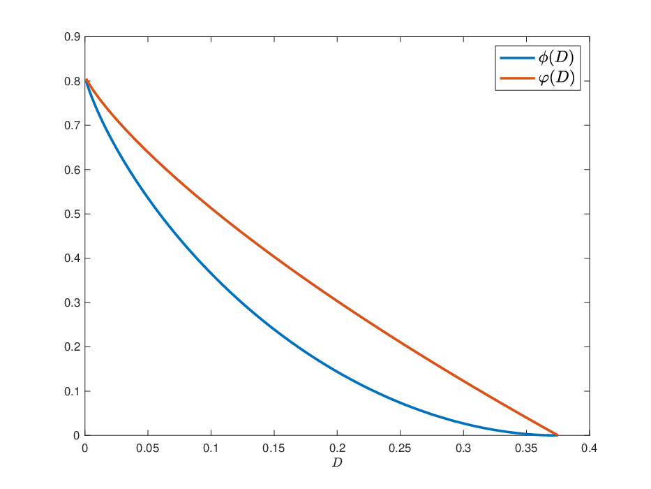
which is in general different from . So [17, Theorem 2] should be interpreted with great caution.
For illustrative purposes, we plot and for in Fig. 1.
Proof:
The expression of can be specialized from [2, Equation (6)]. The derivation of is given in Appendix G. ∎
Theorem 8.
For ,
under the squared distortion measure.
Remark 10.
In this case, and consequently [17, Theorem 2] holds. Indeed, we can deduce from [18, Theorem 1] that
which coincides with .
For illustrative purposes, we plot and for in Fig. 2.

IV Alternative Formulations of the Perception Constraint
The fact that the perception constraint in (5) fails to capture the notion of strong-sense perpect perceptual quality motivates us to consider the following alternative formulation.
Definition 4.
Given distortion constraint and perception constraint , rate is said to be achievable with common randomness if for all sufficiently large , there exist shared seed distribution (on a Polish space), encoding distribution (with countable), and decoding distribution (with ) such that the induced joint distribution satisfies
| (23) |
The infimum of such achievable is denoted . In the case of private randomness only, the corresponding limit is denoted .
Note that the strong-sense perceptual quality constraint can be viewed as an extreme case of the new formulation since setting in (23) forces . So we have and . However, the multiletter nature of the perception constraint in (23) makes it challenging to obtain a computable characterization of and when . To ease the difficulty, we shall impose some further restrictions on :
Assumption 4.
is tensorizable in the sense that
where denotes the joint distribution formed by the product of marginals .
Assumption 5.
is decomposable in the sense that
Note that Assumptions 4 and 5 are satisfied by the Kullback-Leibler divergence and those taking the form of with an additive cost function in the sense for some (e.g., ).
Proof:
We first prove the converse part. Let be an achievable rate with respect to distortion constraint and perception constraint . We have
| (24) |
where is uniformly distributed over and independent of . Moreover,
| (25) |
and
| (26) | ||||
| (27) | ||||
| (28) |
where (26) and (27) are due to respectively the tensorizability and convexity (in its second argument) of . Combining (24), (25), (28) and invoking the fact that proves .
Now it remains to prove the achievability part. We augment into a joint i.i.d. process using a memoryless channel satisfying and . For any positive integer ,
where the equality follows by the decomposability of . Moreover, by the strong functional representation lemma [14], there exists a random variable , independent of , such that can be expressed as a deterministic function of and
Setting and sending completes the proof. ∎
Theorem 10.
For and ,
where
| subject to | |||
Proof:
Suppose that is constrained to be an i.i.d. sequence with marginal distribution satisfying . For such ,
where the equality follows by the decomposability of . Now the problem is converted to output constrained lossy source coding in the sense of [10], and consequently the desired upper bound can be deduced by following steps similar to those for the achievability part of [16, Theorem 2].
It can be shown that, with the output constrained to be i.i.d., this upper bound is in fact the best possible (assuming is tensorizable, decomposable, and convex in its second argument). Moreover, when , the i.i.d. constraint is automatically satisfied and the upper bound is tight. Indeed, we have , which is known to coincide with (or equivalently, ) according to Theorem 6. On the other hand, it is unclear whether the i.i.d. constraint is redundant when . So the upper bound can potentially be loose in that regime. In constrast, as the proof of Theorem 9 indicates, with the presense of common randomness, the i.i.d. constraint incurs no penalty in terms of the rate-distortion-perception tradeoff. ∎Roughly speaking, distortion measures and perception measures in the rate-distortion-perception framework can be considered full-reference metrics and no-reference metrics, respectively. Take image compression as an example. To evaluate a compressed image, full-reference metrics compare it to the ground truth (i.e., the original version) while no-reference metrics quantify its quality using a prescribed criterion based on some statistical feature information. In the current setting, the realization of , the realization of , and the distribution of correspond to the object to be evaluated, the ground truth, and the statistical feature information, respectively. However, the perception constraint in the form of (5) or (23) is imposed on the distribution of , not on its realization. This is somewhat unsatisfactory since the perceptual quality should be defined for each individual object (say, an image) rather than for an ensemble only. Furthermore, it is often impossible to deduce a realization-based perceptual quality measure from a distribution-based measure because two different distributions may generate the same realization. So the operational meaning of (5) and (23) is not entirely clear.
To gain a better understanding, let us revisit the toy example in Section I. Suppose we want to evaluate the “perceptual quality” of a given realization of . Clearly, it is irrelevant here whether the distribution on the unit circle is uniform or not as we are dealing with a property of the realization itself. When a particular realization is concerned, the only role of the so-called “perfect perceptual quality constraint” is to force it to be on the unit circle. So the “perception constraint” should be better stated to specify a perceptually admissible set rather than the distribution(s) on it. Interestingly, if no restriction is imposed on how is distributed on the unit circle, then one can simply choose two antipodal reconstruction points (e.g., those highlighted with in Fig. 3) and perform vector quantization without involving extra randomness. Indeed, deterministic encoding and decoding
yields
previously only achievable with the aid of common randomness. Note that requiring to reside on the unit circle is not a superfluous “perception constraint” since otherwise it is possible [11] to achieve
by using the following modified decoder
with the two reconstruction points (highlighted with in Fig. 3) sitting inside the unit circle. Therefore, this distribution-oblivious “perception constraint” also requires a compromisation of distortion.

By now it should be clear that the role of realization-based perception constraints is to specify a collection of perceptually admissible sets parameterized by (the smaller is, the more restrictive the set becomes). One can reconcile such constraints with their distribution-based counterparts using empirical distribution as a link. To this end, we quantify the perceptual quality of a given realization by the divergence , where is the empirical distribution of . We say is -typical with respect to if , and let the perceptually admissible set be the set of -typical sequences. It will be seen that the single-letter characterization of the rate-distortion-perception function with distribution-based perception constraints (especially in the form of (5)) can be largely recovered in the realization-based framework under the following definition.
Definition 5.
Given distortion constraint and perception constraint , rate is said to be achievable with common randomness if for all sufficiently large , there exist shared seed distribution (on a Polish space), encoding distribution (with countable), and decoding distribution (with ) such that the induced joint distribution satisfies
| (29) |
The infimum of such achievable is denoted . The achievable rate with private randomness is defined in the same way except that the encoder and the decoder do not have access to a shared random seed (i.e., is set to be a constant); the corresponding fundamental limit is denoted . If the encoder and the decoder are further required to be deterministic (i.e., no randomness is allowed at all), we denote the fundamental limit by .
Remark 11.
It is worth mentioning that is in general not feasible under Definition 5 since cannot be realized as an empirical distribution for all sufficiently large . Moreover, implies almost surely. Note that in the finite alphabet case, almost surely for all sufficiently large if and only if
where means is absolutely continuous with respect to .
Proof:
First consider the case of common randomness. Let be an achievable rate with respect to distortion constraint and perception constraint . Similarly to (24) and (25), we have
| (30) | ||||
| (31) |
where is uniformly distributed over and independent of . Note that given , the distribution of is the same as the empirical distribution of , and consequently
Since almost surely and is convex in its second argument, it follows that
| (32) |
Combining (30), (31), (32) and invoking the fact that proves .
Next consider the case of no randomness. According to Assumption 2, for any , there exists a discrete random variable with its support satisfying and such that
By Lemma 1 in Appendix B, for any , when is sufficiently large, we can find deterministic encoding function and decoding function with the properties
where and is the set of -typical sequences with respect to . Clearly, by choosing , we have
Moreover, since is continuous in over the interior of the probability simplex defined on , it follows that
for all when is small enough. Now sending and invoking the continuity of for and shows . In view of the fact that , the proof is complete. ∎Although defining the perceptual quality of a realization based on its empirical distribution is arguably justifiable for i.i.d. sources, this is at best a first-order approximation of what humans subconciously adopt for image evaluation. How to take into account more sophisticated patterns while maintaining the theory at a manageable level is a challenge to be addressed in future works.
V Conclusion
The roles of common randomness and private randomness in rate-distortion-perception theory have been investigated and shown to depend critically on how the perception constraint is formulated. The operational meanings of various perception constraints are also examined. It is our opinion that, as the distinguishing feature of the new theory and likely the decisive factor for its success, the notion of perceptual quality remains to be formalized more convincingly in an information-theoretic framework as a no-reference metric closely mimicking the relevant human intuition.
Appendix A Verification of Assumption 2
Here we verify Assumption 2 for the case , , and (in this case, is written as according to the convention).
Let be a quantized version of , obtained by mapping to its nearest point in , where is a positive integer. Since , for any , we can choose a sufficiently large such that . Let be the mirror version of with respect to in the sense that and . Obviously, form a Markov chain and . Note that
Therefore, we have44 4 It is worth mentioning that the value of does not depend on the choice of divergence . . Since for , it follows that (7) holds.
By the definition of , for any and , there exists a random variable such that
Let be a quantized version of , obtained by mapping to its nearest point in , where is a positive integer. Clearly, we have since . With this construction, (8) is a simple consequence of the data processing inequality. It can be verified that
| (33) | ||||
| (34) | ||||
where (34) is due to the Cauchy-Schwarz inequality. Similarly,
Since (implied by the fact and ), it follows that as . Therefore, we can ensure (9) and (11) by setting large enough. Moreover, (10) is satisifed because
| (35) | ||||
where (35) is due to the Cauchy-Schwarz inequality. In view of the fact that for all with support , (12) must hold as well. This completes the verification of Assumption 2.
Appendix B Proof of Theorem 2
Lemma 1.
Let be a discrete random variable defined on and jointly distributed with and assume that its support satisfies and
Given any , , and , there exist deterministic encoding function and decoding function for all sufficiently large such that
where and denotes the set of -typical sequences with respect to , i.e., .
Proof:
This result has many known variants in the literature (see, e.g., [20, Theorem 9.6.2]). We include its proof for completeness.
We indepenently and uniformly choose codewords from . Given , the encoder finds an such that
| (36) |
If no such exists, the encoder simply sets . Let
where . Given , the encoder fails to find a codeword satisfying (36) only if for all . Therefore,
| (37) | ||||
| (38) |
where (37) is due to [15, Lemma 13.5.3]. Let . It follows from (38) that
where , , are independent and distributed according to . Note that with high probability when is large. Moreover, in light of the weak law of large numbers, and converge, respectively, to and in probability. It is easy to see that
So by choosing , we have as . It is also clear that as .
As shown by the above argument, for any and , when is sufficiently large, we can find deterministic encoding function and decoding function such that
Let
and , . We have
Note that
Since
it follows by the dominated convergence theorem that as . Therefore, by choosing a sufficiently small , we can ensure that , , and consequently
This completes the proof of Lemma 1. ∎Now we proceed to prove Theorem 2. It suffices to consider the case where does not assign all probability mass to a single atom since otherwise the problem is trivial.
According to Assumption 2, for any , there exists a random variable with its support satisfying and such that
| (39) | ||||
By Lemma 1, for any , when is sufficiently large, we can find deterministic encoding function and decoding function with the properties
Clearly, by choosing , we have
Moreover, must converge to under the total variation distance (i.e., ) as given the fact that
Since is continuous in over the interior of the probability simplex defined on , it follows that
| (40) |
when is sufficiently close to zero.
However, in general (40) does not imply the stronger requirement
Nevertheless, there is a simple remedy with the availability of common randomness. For any integer , let be a circular shift operator in the sense that for all , where is modulo- addition55 5 We assume the output of the modulo- operation is in .. Let denote the codebook obtained by applying to every codeword66 6 The resulting codeword still retains the index of the original codeword. of , . Moreover, we equip each codebook with encoding function and decoding function defined as follows:
Note that we have , , and . Let be uniformly distributed over , independent of , and available at both the encoder and decoder. The role of is to specify which codebook (as well as the associated encoding and decoding functions) to use. Let denote the reconstruction. Based on our construction, it is clear that
and consequently
It remains to eliminate common randomness. The key observation here is that can be simulated using a negligible fraction of source symbols as is sublinear in . Specificaly, consider the case where source symbols are leveraged to simulate , where is small enough. Let denote the maximum probability value of (i.e., the maximum of the probabilities of atoms if atoms exist; otherwise, ). We assume since otherwise can be exactly generated from . Obviously, the maximum probability value of is , which vanishes exponentially as (for any given ). This ensures that there is a map such that the distribution of satisfies for all . For example, first map as many atoms as possible to the elements of while ensuring that the total mass of atoms mapped to each element is no greater than ; then use the remaining atoms and atomless measurable sets to fill the gap between the total mass for each element and the target so that the total mass for each element is within the range . Consequently, we have as .
We assume the encoder uses this simulation code on the -th to -th source symbols to generate . It then transmits to the decoder losslessly with bits and applies the aforementioned randomly shifted code to the first source symbols but with replaced by its approximate version . Denote the reconstructions of the first source symbols by . For the -th to -th source symbols, the decoder generates reconstructions , . Under this construction, both the encoder and decoder are deterministic.
We shall show that the deterministic code has the desired properties. Since
it follows that
for all sufficiently large as long as is chosen small enough. Moreover, in view of the fact that , , and as , we must have uniformly for all as , which, together with the uniform convergence of , , to under the total variation distance as and the continuity of in this second argument at , implies
for all sufficiently large as long as is chosen small enough. Finally, invoking the fact that as and the continuity of for and completes the proof of Theorem 2.
Remark 12.
It is possible to avoid using the simulation code via a more careful construction.
Let and . Moreover, we partition into such that , . (The existence of such a partition will be discussed later.)
Take codebook and its associated deterministic encoding function and decoding function as specified in the proof of Theorem 2. Given , the encoder finds77 7 Use a prescribed deterministic tie-break rule if the minimizer is not unique. such that
where . It then sends to the decoder, which produces as the reconstruction. For , , the encoder finds the index pair for the corresponding in according to the aforedescribed encoding rule and sends it to the decoder. The decoder first produces the reconstruction for according to the aforedescribed decoding rule, then outputs the final result by shifting this reconstruction using . Let denote the output induced by this new coding scheme. Since the distortion does not increase for any realization as compared to the original scheme88 8 If we modify the coding scheme by setting for , then the distortion might increase for ., it follows that
| (41) |
where . Moreover, as shown at the end of Appendix B,
| (42) |
So with chosen small enough, the circular symmetry of the coding scheme (conditioned on ) ensures that , , are uniformly close to under the total variation distance and consequently
for all sufficiently large . As the rate overhead for transmitting is negligible, the new coding scheme indeed has the desired properties.
However, there is a subtle issue regarding the partition of into . The existence of such a partition is in a certain sense guaranteed. Note that is the union of a collection of disjoint equivalent classes, where each equivalent class consists of different sequences that can be converted from one to another via circular shifting. We can form by choosing one sequence from each equivalent class in ; then is uniquely specified due to the requirement , . It can be seen that there is considerable freedom in creating this kind of partitions. When is finite or countably infinite, the resulting sets are always measurable. But in a more general setting, certain partitions might yield non-measurable sets.
Here we show that this issue can be resolved by performing the partition judiciously when is a Polish space (as assumed throughout this paper). First consider the case . We shall start with a simple example where . There are totally permutations on , namely, , , , , , and . Pick two permutations that are not related via circular shifting99 9 For example, and are not related via circular shifting while and are since applying to gives .. Each permutation can be used to specificy a region in according to the following rule: . Now we can let be the union of the regions specified by the two picked permutations with the elements in excluded. Then and are also uniquely determined. In general, there are permutations on . We can pick permutations that are not related via circular shifting, and use these permutations to specify regions in (according to the obvious extension of the aforementioned rule). Then define by taking the union of these regions and excluding the elements in . It can be verified that the induced partition is free of the measurability issue.
This method can be generalized to any Polish space. Note that any Borel space on a Polish space is Borel isomorphic to a measurable subspace of . We can simply map the Polish space to a measurable subspace of via an isomorphism , which naturally induces a map from to via the isomorphism . We then perform the partition for the high probability subset of as above, and take intersections to produce a partition for the high probability subset of . Mapping this back to the Polish space , we obtain a desired partition.
Proof of (42): Note that given , we can divide into subsets of size , and the elements in each subset differ by a multiple of (modulo-). For example, when and , we have two subsets and . In this case, means and ; as a consequence
where for . In general, it can be verified that implies at least independent events of the kind , which, together with the fact , further implies
Now one can readily prove (42) since
where the last step is due to .
Appendix C Verification of Assumption 3
Here we verify Assumption 3 for the case and .
According to the definition of , for any and , there exists a random variable such that
Let be a quantized version of , obtained by mapping to its nearest point in , where is a positive integer. By the data processing inequality,
As is convex in and consequently1010 10 It is shown in Appendix A that for . continuous for , we have by choosing a sufficiently small . Let be the mirror version of with respect to in the sense that and . Obviously, form a Markov chain and . Moreover,
| (43) | ||||
| (44) | ||||
where (43) is due to the Cauchy-Schwarz inequality, and (44) is due to (implied by the fact that ). Since , it follows that , which further implies as . Therefore, we can ensure by setting large enough. This completes the verification.
Appendix D Proof of Theorem 4
According to Assumption 3, for any , there exist and such that form a Markov chain, the support of , denoted , satisifies , and
We shall treat the conditional distribution induced by specified above as a memoryless channel and establish a soft-covering lemma that is needed for the proof of Theorem 4.
Definition 6.
Given a codebook , let denote its induced distribution of the output sequence generated through memoryless channel by a codeword randomly picked from according to the uniform distribution.
Lemma 2.
For any and , there exists a sequence of codebooks with and such that
where denotes the set of -typical sequences with respect to .
Proof:
We first briefly review some basic definitions in information-spectrum methods. The limsup in probability of a sequence of random variables is defined as
Correspondingly, the liminf in probability is defined as
For a sequence of pairs of random variables , the sup-information rate of is defined as
where denotes the information density of . For a sequence of distributions , the inf-relative-entropy rate of is defined as
Now we are in a position to prove Lemma 2. Construct a sequence of pairs of random variables with and another sequence of pairs of random variables with , where and is a truncated version in the sense that
By the general soft-covering lemma [21, Theorem 4][22, Corollary VII.4], for any , there exists a sequence of codebooks with and such that
Note that
| (45) | ||||
where (45) is due to the data processing inequality for the total variation distance. Moreover, in light of the triangle inequality for the total variation distance,
So it suffices to prove .
It can be verified that
| (46) | ||||
where (46) follows by [23, p. 14, the third inequality from the bottom]. Since and the conditional distribution of given is the same as , we must have
Moreover, by the weak law of large numbers,
Finally, invoking the fact that [23, Lemma 3.2.1] completes the proof of Lemma 2. ∎
Now we proceed to prove Theorem 4. Given and , let be a sequence of codebooks with the properties specified in Lemma 2. Construct by applying the shift operator to every codeword of , . Let be uniformly distributed over , and be uniformly distributed over given , . Denote the output sequence generated by through memoryless channel as . For ,
| (47) | ||||
where (47) holds because is simply a shifted version of while is shift-invariant. Since is convex in its first argument, it follows that
and consequently must converge to as .
Our coding scheme can be illustrated using the following probablistic graphical model:
The encoder first leverages the conditional distribution induced by to generate based on . Note that we have , , and . For ,
| (48) | ||||
| (49) | ||||
where (48) and (49) are due to the triangle inequality and the data processing indequality for the total variation distance, respectively. Furthermore, we have as , and uniformly for all as . Therefore,
for and all sufficiently large , where as .
For each , let1111 11 Since is shift-invarint and is memoryless, it follows that and consequently are shift-invariant as well, which further implies the shift-invariance of in view of the fact . Therefore, , , , , , and are all time-invariant.
where
We claim that is a regular conditional distribution. Indeed, on one hand, given each , is a distribution (more precisely, a probability mass function) since , , and
on the other hand, given each , is measurable (which is due to the fact that both and are measurable), and so is for each . Moreover, given each , is in fact a maximal coupling of and since
which clearly also holds when .
The encoder leverages induced by to generate from , . Note that and
when is sufficiently large.
The encoder then sends to the decoder. We have
| (50) | ||||
| (51) |
where (50) is due to Fano’s inequality, and (51) holds when and is sufficiently large.
Given , the decoder simply generates using the conditional distribution . It is clear that , , and consequently
Finally, by choosing sufficiently small, sufficiently close to , and sufficiently large, we can make
as close to as we want. This completes the proof of Theorem 4.
Appendix E Verification of Uniform Integrability
Here we verify uniform integrability for the case , , and .
By the Cauchy-Schwarz inequality,
Note that for any ,
Similarly, we have
Since and , it follows by the dominated convergence theorem that both and converge to as . Therefore, there exists such that and . Setting ensures
Appendix F Proof of Theorem 6
We shall first prove . For any satisfying (17), (18), and (19), let and . Since form a Markov chain (see (18)), it follows that
which, together with (17), implies
Now consider the case . Note that
| (52) | ||||
where (52) is due to the data processing inequality. By symmetry (see (19)), continues to hold if . This proves .
Appendix G Proof of Theorem 7
In view of (20), the problem boils down to determining by solving the optimization problem in (21). To this end, we need the following lemma.
Lemma 3.
If there exist over a finite set with , , and such that
| (53) | ||||
| (54) | ||||
| (55) |
then given by
is an optimal solution to (21).
Proof:
It is clear that there is no loss of generality in assuming that only takes value from . Let be an arbitrary finite subset of . In view of the standard Karush-Kuhn-Tucker conditions [15, pp. 362–364], (53)–(55) ensures that attains the infimum in (21) when the alphabet of is restricted1212 12 We set for . to be . Moreover, according to the support lemma [24, p. 631], it suffices to consider the finite alphabet case; in fact, the alphabet size of does not need to exceed for the purpose of preserving , , and . So must be an optimal solution to (21). ∎Now we are in a position to solve (21). It suffices to consider the case since obviously equals when and equals when .
Let with
Note that . Define over such that
Moreover, let
which is clearly positive. We shall proceed to verify that the constructed and satisfying (53)–(55).
Next let
We have
Clearly,
if and only if
where
It can be verified that
On the other hand,
Moreover,
which shows that is a strictly convex function for and a strictly concave function for . So we must have
and consequently
References
- [1] Y. Blau and T. Michaeli, “The perception-distortion tradeoff,” in Proc. IEEE Conf. Comp. Vision and Pattern Recog. (CVPR), 2018, pp. 6288–6237.
- [2] Y. Blau and T. Michaeli, “Rethinking lossy compression: The rate-distortion-perception tradeoff,” in International Conference on Machine Learning, pp. 675–685, 2019.
- [3] L. Theis and A. B. Wagner, “A coding theorem for the rate-distortion-perception function,” ICLR 2021 neural compression workshop.
- [4] R. Matsumoto, “Introducing the perception-distortion tradeoff into the rate-distortion theory of general information sources,” IEICE Comm. Express, vol. 7, no. 11, pp. 427–431, 2018.
- [5] R. Matsumoto, “Rate-distortion-perception tradeoff of variable-length source coding for general information sources,? IEICE Comm. Express, vol. 8, no. 2, pp. 38–42, 2019.
- [6] M. Li, J. Klejsa, and W. B. Kleijn, “Distribution preserving quantization with dithering and transformation,” IEEE Signal Process. Lett., vol. 17, no. 12, pp. 1014–1017, Dec. 2010.
- [7] M. Li, J. Klejsa, and W. B. Kleijn. (2011). “On distribution preserving quantization. [Online]. Available: http://arxiv.org/abs/1108.3728
- [8] J. Klejsa, G. Zhang, M. Li, and W. B. Kleijn, “Multiple description distribution preserving quantization,” IEEE Trans. Signal Process., vol. 61, no. 24, pp. 6410–6422, Dec. 2013.
- [9] N. Saldi, T. Linder, and S. Yüksel, “Randomized quantization and source coding with constrained output distribution,” IEEE Trans. Inf. Theory, vol. 61, no. 1, pp. 91–106, Jan. 2015.
- [10] N. Saldi, T. Linder, and S. Yüksel, “Output constrained lossy source coding with limited common randomness,” IEEE Trans. Inf. Theory, vol. 61, no. 9, pp. 4984–4998, Sep. 2015.
- [11] L. Theis and E. Agustsson, “On the advantages of stochastic encoders,” ICLR 2021 neural compression workshop.
- [12] I. Csiszár and P. C. Shields, “Information theory and statistics: A Tutorial”, Foundations and Trends in Communications and Information Theory, vol. 1, no. 4, pp. 417–528, 2004.
- [13] V. van Erven and P. Harremoës, “Rényi divergence and Kullback-Leibler divergence,” IEEE Trans. Inf. Theory, vol. 60, no. 7, pp. 3797–3820, Jul. 2014.
- [14] C. T. Li and A. El Gamal, “Strong functional representation lemma and applications to coding theorems,” IEEE Trans. Inf. Theory, vol. 64, no. 11, pp. 6967–6978, Nov. 2018.
- [15] T. M. Cover and J. A. Thomas, Elements of Information Theory. New York, NY, USA: Wiley, 1991.
- [16] A. B. Wagner, “The rate-distortion-perception tradeoff: The role of common randomness,” 2022, arXiv:2202.04147. [Online] Available: https://arxiv.org/abs/2202.04147
- [17] Z. Yan, F. Wen, R. Ying, C. Ma, and P. Liu, “On perceptual lossy compression: The cost of perceptual reconstruction and an optimal training framework,” in International Conference on Machine Learning, 2021.
- [18] G. Zhang, J. Qian, J. Chen, and A. Khisti, ”Universal Rate-Distortion-Perception Representations for Lossy Compression,” in Conference on Neural Information Processing Systems, 2021.
- [19] H. Liu, G. Zhang, J. Chen, A. Khisti, “Lossy compression with distribution shift as entropy constrained optimal transport,” in International Conference on Learning Representations, 2022.
- [20] R. Gallager, Information Theory and Reliable Communication. New York, NY, USA: Wiley, 1968.
- [21] T. S. Han and S. Verdú, “Approximation theory of output statistics,” IEEE Trans. Inf. Theory, vol. 39, no. 3, pp. 752–772, Mar. 1993.
- [22] P. Cuff, “Distributed channel synthesis,” IEEE Trans. Inf. Theory, vol. 59, no. 11, pp. 7071–7096, Nov. 2013.
- [23] T. S. Han, Information-Spectrum Methods in Information Theory. Springer, 2003.
- [24] A. El Gamal and Y.-H. Kim, Network Information Theory. Cambridge, U.K.: Cambridge Univ. Press, 2011.