Highly-transmitting modes of light in dynamic atmospheric turbulence
Abstract
We show that instantaneous spatial singular modes of light in a dynamically evolving, turbulent atmosphere offer significantly improved high-fidelity signal transmission as compared to standard encoding bases corrected by adaptive optics. Their enhanced stability in stronger turbulence is associated with a subdiffusive algebraic decay of the transmitted power with evolution time.
Introduction.— Wave transport in random scattering media is ubiquitous in communication, sensing and imaging, from astronomical F. Roddier 2004 over mesoscopic G. Labeyrie et al. 1999; Popoff et al. 2014; Hsu et al. 2017 to microscopic scales Dorokhov 1984. In all these rather diverse physical settings, the common goal is to faithfully transmit and filter relevant information generated by the sender, probed by the scattering wave, or emitted by some unknown object(s). To achieve an efficient transmission and retrieval of information, it is indispensable to mitigate the random, i.e., uncontrolled modulation of the transmitted signal’s phase and intensity profile.
In the atmosphere, the primary sources of uncontrolled light modulations are turbulent eddies, i.e. blobs of air with smoothly varying refractive index. On the one hand, the minimal size of turbulent eddies is much larger than optical wavelengths Michael C. Roggemann et al. 1997, accordingly scattering on such eddies occurs mainly in the forward direction Fante 1975. On the other hand, the eddies’ sizes are comparable to the typical transverse width of propagating beams Michael C. Roggemann et al. 1997, resulting in random phase shifts of the light’s transverse profile Fante 1975. Furthermore, a combination of refraction and diffraction gives rise to intensity fluctuations upon transmission Fante 1975. Although phase errors can be compensated by adaptive optics (AO) Michael C. Roggemann et al. 1997; F. Roddier 2004; Y. Ren et al. 2014; Y. Ren et al. 2016; J. Zhao et al. 2020; Tyson 2016, the latter cannot alleviate intensity fluctuations G. Sorelli et al. 2019. Nor can AO reduce transmission losses arising due to finite-size apertures.
We propose to exploit the medium’s intrinsic properties for signal transmission across random disorder: Wave propagation in static disordered media generically allows for the formation of highly-transmitting spatial modes S. Rotter and Gigan 2017; Segev et al. 2013; Yılmaz et al. 2019. These modes qualify due to their minimal transverse losses as ideal candidates for high-dimensional signal encoding. However, their stability is challenged in a dynamically evolving medium – here the Earth’s atmosphere. Yet, even in the time-dependent atmosphere the channel’s geometry and turbulence parameters remain invariant. Therefore, one can expect that certain robust features are inscribed into instantaneous modes lending them persistent stability properties. Our present purpose is to consolidate this expectation, and to quantify the time scales over which such highly-transmitting modes offer resilient signal transmission with reduced losses.
The model.— We consider the horizontal propagation of a monochromatic laser beam through a clear atmospheric channel (e.g., free of fog or clouds), limited by two coaxial circular source and receiver apertures with diameters and , respectively, see Fig. 1. We study the spatial field distribution of the propagating beam, and choose a wavelength of nm which is in the infrared transparency window of the Earth’s atmosphere Kopeika 1998; Andrews 2005. Furthermore, we consider propagation distances much shorter than the light’s transport mean free path Carminati and Schotland 2021; mea, thereby neglecting the small attenuation of the field due to molecular and aerosol absorption and scattering Andrews 2005; Kopeika 1998. In this case, the propagation of a scalar light wave obeys the stochastic parabolic equation Andrews 2005

| (1) |
where , – the transverse Laplace operator with respect to the propagation axis – accounts for wave diffraction, and is the fluctuating part of the refractive index of air, to model the random turbulent potential and its time dependence.
The statistical properties of in Eq. (1) are governed, according to Kolmogorov theory Kolmogorov 1941, by the refractive index power spectrum , where denotes the transverse spatial frequency of refractive index fluctuations. These random inhomogeneities of the refractive index induce phase distortions with typical correlation radius given by the Fried parameter Andrews 2005, which is inversely proportional to the turbulence strength. The Fried parameter typically varies on the timescale of hours Andrews 2005 and can thus be assumed time-independent. Furthermore, phase distortions combined with diffraction give rise to intensity fluctuations, whose strength is quantified by the Rytov variance Tyson 2016; Tatarskii 2016; A. Ishimaru 1978.
For fixed times , the stochastic parabolic Eq. (1) is accurately solved by a split-step method Schmidt 2010; Lukin 2002; G. Sorelli et al. 2019, which relies on segmenting the propagation path into discrete, medium-induced phase modulations, i.e., phase screens, equally interconnected by vacuum diffraction (Fig. 1). Although every elementary propagation step of length only introduces phase errors sup, the assembled path reliably models as well intensity fluctuations which originate from constructive or destructive interference. To implement this numerically, we employ Fourier optics methods Born and Wolf 1999; Goodman 2005; Schmidt 2010; E. M. Johansson and Gavel 1994 and standard phase screens Schmidt 2010; E. M. Johansson and Gavel 1994 augmented by Zernike polynomials N. A. Roddier 1990.
Mathematically, the combination of phase distortions and free diffraction can be represented by the unitary operator acting on the propagating wave; the geometric truncation due to source and receiver apertures (Fig. 1) are captured by projection operators and , respectively. Combined, this defines the channel’s turbulence operator which maps modes from the source space onto the receiver space . In general, this operator is non-unitary, since light escapes the receiver aperture due to diffraction, turbulence-induced broadening and beam wandering Andrews 2005.
By performing a singular value decomposition (SVD) S. Rotter and Gigan 2017; D. A. B. Miller 2019 of , we find its orthonormal transmission channels: Source modes with mode index are coupled bijectively to receiver modes , each associated with singular values quantifying the transmitted power per channel, where and are transverse position vectors in the source and receiver apertures. The action of on an input state thus has the explicit form
| (2) |
where denotes the convolution, stands for the standard scalar product in transverse space, and the number of singular modes with non-vanishing weight depends on the source and receiver apertures’ cross sections. Practically, the SVD is applied to a matrix representation of the turbulence operator, known as transmission matrix , where and are basis modes on the source and receiver side, respectively. For an accurate representation of transmitted fields confined by circular apertures, we choose Laguerre-Gaussian (LG) modes at the source side, which also feature convenient diffraction properties Andrews 2005. To resolve the fine details of turbulence-induced distortions imprinted into the receiver modes a large number of pixel modes is employed at the receiver’s end. All parameters of our model our lacka are chosen to match realistic experimental conditions Lavery et al. 2017; M. Krenn et al. 2015.
Properties of instantaneous singular modes.— Before considering dynamical turbulence, we investigate the statistical properties of singular modes associated with an instantaneous atmospheric realization. The average distribution of singular values over an ensemble of random realizations is known in the asymptotic regime of weak turbulence J. H. Shapiro 1974 and aligns with our results. But our present numerical approach captures the properties of the singular modes under general, non-asymptotic turbulence conditions, and thus considerably expands over earlier studies J. H. Shapiro 1974; J. M. Kahn and Belmonte 2018; L. Borcea et al. 2020; V. N. Shatokhin et al. 2020. Representative examples of intensity and phase distributions of highly-transmitting (i.e., associated singular values close to one) source (a) and receiver (b) singular modes are shown in Fig. 2, for three values of corresponding to the regimes of weak, moderate and strong intensity fluctuations (left to right).
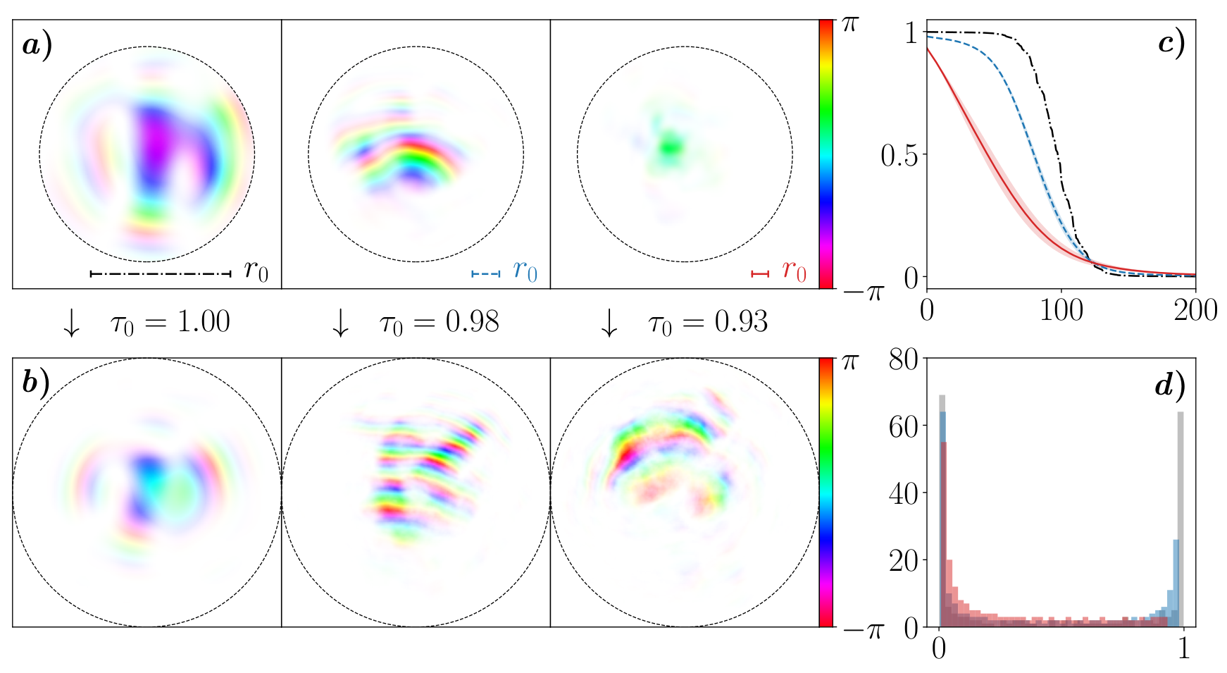
We note that with increasing turbulence strength, the source modes occupy smaller transverse areas. In addition, non-trivial phases of both, the source and receiver modes [encoded in the color gradient in Fig. 2(a,b)] are another salient feature – highlighting the relevance of constructive interference effects for effective transmission.
The right-hand panels of Fig. 2 show the distribution of singular values (c) and its histogram (d) after ensemble averaging over 500 atmospheric realizations. The black dash-dot curve corresponds to weak intensity fluctuations initially leveling for approximately 80 perfectly-transmitting singular modes associated with (the overline designates the ensemble average). The performance of further singular modes drops quickly towards vanishing transmittance, i.e., , where the wiggles in the curve reflect residual degeneracy of singular values stemming from geometric symmetries in the absence of turbulence D. A. B. Miller 2019. This sharp separation between open () and closed channels () corresponds to a bimodal distribution [Fig. 2(d)] and agrees with the singular value distribution observed in the absence of D. Slepian 1965 or in weak turbulence J. H. Shapiro 1974, as well as in other complex scattering systems Dorokhov 1984; Nazarov 1994; Beenakker 1997. However, with increasing turbulence strength the open channels evolve into partially transmitting channels, i.e., Goetschy and Stone 2013; Popoff et al. 2014; Hsu et al. 2017. With increasing turbulence strength the open-channel plateau shrinks (blue dashed line in Fig. 2 for moderate intensity fluctuations) and eventually turns into a monotonic decay (red solid line) of the transmittance for strong intensity fluctuations. In the latter regime, the resulting unimodal singular value distribution [Fig. 2(d)] is dominated by closed channels. Notwithstanding, even in this case, we identify more than ten modes with singular values .
Stability in dynamic turbulence.— Given the non-negligible set of highly-transmitting modes – even in strong turbulence – we need to address their stability under the atmosphere’s dynamical evolution. To account for the latter, we adopt Taylor’s hypothesis G. I. Taylor 1935, which states that the short time (s) atmospheric evolution is described by the wind-induced transverse flow of static turbulent eddies Andrews 2005. Within the framework of our split-step approach, this behavior is implemented by transverse shifts of individual phase screens with respect to the propagation direction according to appropriate velocity distributions Lukin 2002; E. Anzuola and Gładysz 2017 (cf. Fig. 1). Here, we assume normally-distributed transverse winds with mean and variance which induce atmospheric coherence times F. Roddier 2004.
In general, the atmospheric propagation of highly-transmitting modes associated with some initial realization of turbulence at will yield some unknown field on the receiver’s end for . As seen from Eq. (2), this field has to satisfy the initial condition . Consequently, the mean transmitted power is given by with , and a mode’s stability may be characterized by the way decays. Moreover, the evolution of the mean crosstalk matrix, quantifies the dynamically induced, undesired transfer of power from into other output modes. We benchmark this stability against the performance of optimized LG modes 11 1 The LG beam waist mm is chosen to maximize transmission in vacuum. For the definitions of transmitted power and crosstalk of LG modes denotes the azimuthal index and is given by modes propagated through evolved turbulence at time while corresponds to LG modes propagated through vacuum. subject to ideal AO corrections G. Sorelli et al. 2019. This means all phase errors attained by a propagated plane wave are subtracted form the received LG modes.

The main panel of Fig. 3 compares the mean transmitted power of the singular mode with the highest transmittance (; blue) to the AO corrected Gaussian (i.e., LG, ) mode (red) in the regime of strong intensity fluctuations, i.e., . The transmitted power is plotted as a function of time in units of , which renders the temporal dynamics of power transmittance and crosstalk independent of the mean wind speed . First, we observe that the Gaussian mode (red line in Fig. 3), being independent of the turbulent medium, transfers the same power on average. In contrast, being optimized for the initial realization of the turbulent medium, singular modes transmit less and less power as the atmosphere evolves. Nevertheless, it is evident from Fig. 3 that the singular mode with the largest singular value outperforms the power transmission of the Gaussian mode for sufficiently short time scales , where denotes the time when the transmitted powers of singular modes and LG modes intersect.
We establish by careful fits that the singular modes’ transmitted power is governed by the following decay law:
| (3) |
where the mean transmitted power at is given by the averaged singular values , while represents the asymptotic limit , obtained by propagating the singular modes through uncorrelated (rather than wind-shifted, see Fig. 1) phase screens. The parameters , and (for ) are instead determined through non-linear fits for different turbulence strengths sup. In particular, ( and ) are obtained by fitting the numerical data for (), where the crossover time is the inflection point of , which is inversely proportional to the mean wind speed, determined by the channel geometry and independent of the mode number sup.
The short-time decay in Eq. (3) is similar to the known decay law of the Strehl ratio F. Roddier 2004, a quantifier of imaging quality in optics Tyson 2016; Born and Wolf 1999. Notably, we find this initial decay to be universal: is independent of the Fried parameter , of the mean transverse wind speed – due to rescaling with – and of the mode number . In other words, the initial rate of a mode’s transmittance loss is solely determined by the static channel geometry, while its duration is fixed by the mean transverse wind speed .
The subsequent algebraic decay of transmitted power for is subdiffusive, i.e. decays slower than . For the eleven highest-transmitting singular modes and various turbulence strengths we find sup. This slow decay may be attributed to long-range transverse spatial correlations due to the Kolmogorov turbulence power spectrum Kolmogorov 1941; Andrews 2005: By means of Taylor’s hypothesis Kolmogorov’s long-ranging spatial correlations are translated into slowly decaying temporal correlations inducing the slow subdiffusive decay of transmittance. To corroborate this hypothesis, we consider light propagation through a disordered medium with only short-range correlations. Phase distortions in such a medium may be described by a Gaussian power spectrum J. M. Martin and Flatté 1988; A. Ishimaru 1978 for which we observe a purely exponential decay of the singular modes’ transmitted power sup.
The temporal stability of singular modes as compared to optimized LG modes is further substantiated by the evolution of their crosstalk matrices (top and bottom rows in Fig. 3, respectively). The coupling among the eleven highest-transmitting singular modes exhibits a prominent diagonal structure for , corresponding to negligible crosstalk. Furthermore, this structure leaves fingerprints even for longer times, while the considered LG modes feature strong crosstalk at all times.
Finally, we assess the effect of intensity fluctuations on the time interval over which singular modes perform better than LG modes. Figure 4 shows the extracted intersection time versus Rytov variance for the two highest transmitting modes ( in blue and in orange) for the same channel geometry as previously. We observe that is a nonlinear, monotonically increasing function of the Rytov variance. Since all of the considered eleven singular modes sup performed similarly well (cf. blue and orange curves for the two highest-transmitting modes in the insets of Fig. 4) and the transmittance of the LG modes decreases quickly for higher mode numbers (cf. red and green curves in the insets), the growth rate of the intersection time increases with the mode number . This is consistent with our above discussion of the distinct crosstalk properties of singular and LG modes (cf. Fig. 3). In particular, it emphasizes the potential benefit of singular modes for multi-mode applications such as high-dimensional information encoding in dynamical disordered media.
Conclusion.— The universality of our approach may open new venues of future research in various directions. For instance, the split-step method and the subsequent decomposition of the transmission matrix may be applied to any channel geometry and any turbulent medium, including non-Kolmogorov models or underwater channels. It would be particularly interesting to examine how our main results are transferred to different dynamic disordered media. Finally, recent experimental efforts have been dedicated to the spatiotemporal characterization of disorder in optical media, see e.g. the measurement of a time-gated transmission matrix in Devaud et al. 2022. We expect that combining these experimental advances with our theoretical tools could lead to new levels of control of light transmission in time-dependent disordered optical media.
Acknowledgements.— The authors are thankful for the fruitful discussions with Szymon Gładysz. We also acknowledge financial support of the Studienstiftung des deutschen Volkes and support by the state of Baden-Württemberg through bwHPC. This work was partially funded by French ANR under COSMIC project (ANR-19-ASTR0020-01). V.S. and A.B. acknowledge partial funding and support through the Strategiefonds der Albert-Ludwigs-Universität Freiburg and the Georg H. Endress Stiftung.
References
- F. Roddier (2004) F. Roddier, Adaptive Optics in Astronomy (Cambridge University Press, Cambridge, 2004).
- G. Labeyrie et al. (1999) G. Labeyrie, F. Tomasi, J. Bernard, C. A. Müller, C. Miniatura, and R. Kaiser, Phys. Rev. Lett. 83, 5266 (1999).
- Popoff et al. (2014) S. M. Popoff, A. Goetschy, S. F. Liew, A. D. Stone, and H. Cao, Phys. Rev. Lett. 112, 133903 (2014).
- Hsu et al. (2017) C. W. Hsu, S. F. Liew, A. Goetschy, H. Cao, and A. D. Stone, Nature Physics 13, 497 (2017).
- Dorokhov (1984) O. N. Dorokhov, Solid State Commun. 51, 381 (1984).
- Michael C. Roggemann et al. (1997) Michael C. Roggemann, B. M. Welsh, and R. Q. Fugate, Rev. Mod. Phys. 69, 437 (1997).
- Fante (1975) R. Fante, Proceedings of the IEEE 63, 1669 (1975).
- Y. Ren et al. (2014) Y. Ren, G. Xie, H. Huang, C. Bao, Y. Yan, N. Ahmed, M. P. J. Lavery, B. I. Erkmen, S. Dolinar, M. Tur, M. A. Neifeld, M. J. Padgett, R. W. Boyd, J. H. Shapiro, and A. E. Willner, Optics Lett. 39, 2845 (2014).
- Y. Ren et al. (2016) Y. Ren, L. Li, Z. Wang, S. M. Kamali, E. Arbabi, A. Arbabi, Z. Zhao, G. Xie, Y. Cao, N. Ahmed, Y. Yan, C. Liu, A. J. Willner, S. Ashrafi, M. Tur, A. Faraon, and A. E. Willner, Sci. Rep. 6, 33306 (2016).
- J. Zhao et al. (2020) J. Zhao, Y. Zhou, B. Braverman, C. Liu, K. Pang, N. K. Steinhoff, G. A. Tyler, A. E. Willner, and R. W. Boyd, Opt. Express 28, 15376 (2020).
- Tyson (2016) R. Tyson, Principles of adaptive optics (CRC Press, Boca Raton, 2016).
- G. Sorelli et al. (2019) G. Sorelli, N. Leonhard, V. N. Shatokhin, C. Reinlein, and A. Buchleitner, New J. Phys. 21, 023003 (2019).
- S. Rotter and Gigan (2017) S. Rotter and S. Gigan, Reviews of Modern Physics 89, 015005 (2017).
- Segev et al. (2013) M. Segev, Y. Silberberg, and D. N. Christodoulides, Nat. Photonics 7, 197 (2013).
- Yılmaz et al. (2019) H. Yılmaz, C. W. Hsu, A. Yamilov, and H. Cao, Nature Photonics 13, 352 (2019).
- Kopeika (1998) N. Kopeika, A System Engineering Approach to Imaging, Press Monographs (SPIE Optical Engineering Press, 1998).
- Andrews (2005) L. Andrews, Laser beam propagation through random media (SPIE, Bellingham, 2005).
- Carminati and Schotland (2021) R. Carminati and J. C. Schotland, Principles of Scattering and Transport of Light (Cambridge University Press, 2021).
- (19) For the propagation distance of km, the power transmittance at nm is about 99% Andrews 2005, which via the Lambert-Beer law yields the transport mean free path km .
- Kolmogorov (1941) A. N. Kolmogorov, Dokl. Acad. Sci. URSS 30, 301 (1941).
- Tatarskii (2016) V. I. Tatarskii, Wave propagation in a turbulent medium (Dover Publications, Mineola, 2016).
- A. Ishimaru (1978) A. Ishimaru, Wave Propagation and Scattering in Random Media (Academic Press, New York, 1978).
- Schmidt (2010) J. Schmidt, Numerical simulation of optical wave propagation with examples in MATLAB (SPIE, Bellingham, 2010).
- Lukin (2002) V. P. Lukin, Adaptive beaming and imaging in the turbulent atmosphere (SPIE, Bellingham, 2002).
- (25) See Supplemental Material for more details of the mean transmitted power of the first eleven singular modes, the fitting procedures and the Gaussian (i.e. non-Kolmogorov) power spectrum .
- Born and Wolf (1999) M. Born and E. Wolf, Principles of optics : electromagnetic theory of propagation, interference and diffraction of light (Cambridge University Press, Cambridge, 1999).
- Goodman (2005) J. Goodman, Introduction to Fourier optics (Roberts & Co, Englewood, 2005).
- E. M. Johansson and Gavel (1994) E. M. Johansson and D. T. Gavel, in Amplitude and Intensity Spatial Interferometry II, edited by J. B. Breckinridge (SPIE, 1994).
- N. A. Roddier (1990) N. A. Roddier, Opt. Eng. 29, 1174 (1990).
- D. A. B. Miller (2019) D. A. B. Miller, Adv. Opt. Photonics 11, 679 (2019).
- our (lacka) Parameters of our channel: km, cm, cm. Source basis: LG modes (beam waist mm, radial and azimuthal indices ); receiver basis: (pixels (a).
- Lavery et al. (2017) M. P. J. Lavery, C. Peuntinger, K. Günthner, P. Banzer, D. Elser, R. W. Boyd, M. J. Padgett, C. Marquardt, and G. Leuchs, Science Advances 3, e1700552 (2017).
- M. Krenn et al. (2015) M. Krenn, J. Handsteiner, M. Fink, R. Fickler, and A. Zeilinger, Proc. Natl. Acad. Sci. U.S.A. 112, 14197 (2015).
- J. H. Shapiro (1974) J. H. Shapiro, Appl. Opt. 13, 2614 (1974).
- J. M. Kahn and Belmonte (2018) J. M. Kahn and A. Belmonte, in Broadband Access Communication Technologies XII, edited by B. B. Dingel, K. Tsukamoto, and S. Mikroulis (SPIE, 2018).
- L. Borcea et al. (2020) L. Borcea, J. Garnier, and K. Sølna, J. Opt. Soc. Am. A 37, 720 (2020).
- V. N. Shatokhin et al. (2020) V. N. Shatokhin, D. Bachmann, G. Sorelli, N. Treps, and A. Buchleitner, in Environmental Effects on Light Propagation and Adaptive Systems III, edited by K. Stein and S. Gladysz (SPIE, 2020).
- D. Slepian (1965) D. Slepian, J. Opt. Soc. Am. 55, 1110 (1965).
- Nazarov (1994) Y. V. Nazarov, Phys. Rev. Lett. 73, 134 (1994).
- Beenakker (1997) C. W. J. Beenakker, Rev. Mod. Phys. 69, 731 (1997).
- Goetschy and Stone (2013) A. Goetschy and A. D. Stone, Phys. Rev. Lett. 111, 063901 (2013).
- G. I. Taylor (1935) G. I. Taylor, Proc. R. Soc. Lond. A 151, 421 (1935).
- E. Anzuola and Gładysz (2017) E. Anzuola and S. Gładysz, Opt. Eng. 56, 1 (2017).
- (44) The LG beam waist mm is chosen to maximize transmission in vacuum. For the definitions of transmitted power and crosstalk of LG modes denotes the azimuthal index and is given by modes propagated through evolved turbulence at time while corresponds to LG modes propagated through vacuum.
- our (lackb) Crosstalk matrices are inset in Fig. 3 at and 21.63. The entries correspond to eleven singular modes (top) or optimized LG modes (bottom), where the vertical axes represent unperturbed modes at and transmitted modes run along the horizontal axes (ordered by transmittance (b).
- our (lackc) m/s and m/s (Gaussian distribution (c).
- J. M. Martin and Flatté (1988) J. M. Martin and S. M. Flatté, Appl. Opt. 27, 2111 (1988).
- Devaud et al. (2022) L. Devaud, B. Rauer, M. Kühmayer, J. Melchard, M. Mounaix, S. Rotter, and S. Gigan, Phys. Rev. A 105, L051501 (2022).
I Supplemental Material
In this Supplemental Material, we provide details of the mean transmitted power (cf. Fig. 3 in the main manuscript) of the first eleven singular modes, i.e., , and for different values of the Fried parameter , ranging from 15 mm to 33 mm (with a mean velocity m/s). Table 1 summarizes the employed turbulence parameters. The number of phase screens required for the split-step method at a given Fried parameter is chosen such that each interval is short enough to remain within the regime of weak intensity fluctuations, i.e., .
| /mm | 15 | 20 | 25 | 33 |
|---|---|---|---|---|
| 6.72 | 4.16 | 2.87 | 1.81 | |
| 25 | 15 | 11 | 7 |
All simulations of the atmosphere relied on the Kolmogorov power spectrum of turbulence Kolmogorov 1941; Andrews 2005
| (4) |
where denotes the transverse spatial frequency of refractive index fluctuations. In this case, we obtain the initial exponential decay of transmitted power which transits into an algebraic decay for larger times, cf. Figs. 5-8 and given in Eq. (7) [Eq. (3) in the main manuscript]. Additionally, we employed a Gaussian (i.e., non-Kolmogorov) power spectrum J. M. Martin and Flatté 1988; A. Ishimaru 1978
| (5) |
where we chose a length scale of mm and seven propagation steps (cf. Table 1) leading to similar turbulence strengths as for the Kolmogorov spectrum with mm. Simulations based on the spectrum given in Eq. (5) entail exponential decay of the transmitted power with time, cf. Fig. 9 and Eq. (8).
To complement Fig. 3 of the main manuscript, Figs. 5-8 are plotted on double logarithmic scales in order to highlight the difference of the two decay regimes. The blue solid curve in each subplot shows the numerically obtained mean transmitted power (with its asymptotic offset subtracted), i.e., , versus time in units of atmospheric coherence times corresponding to singular mode . The offset is found numerically by ensemble averaging the transmitted power of singular modes associated with a given realization of turbulence through a statistically independent realization with the same Fried parameter . The ensemble averaging was performed over at least disorder realizations and the blue error bands correspond to one standard deviation.
The dot-dashed orange and black curves in Figs. 5-8 [atmospheric Kolmogorov spectrum, i.e., Eq. (4)] are obtained by two independent nonlinear fits. Both fitting parameters and their errors are determined with the python library scipy.optimize.curve_fit and the crossover time between the two fitting domains is given by the inflection point of . Since our numerical simulation yields discrete data points, was found by maximization of the difference quotient
| (6) |
The explicit form of the two fitting functions (composing a single piecewise function) reads
| (7) |
Thus, the initial exponential decay [orange dot-dashed curve in Figs. 5-8 and first line of Eq. (7)] for was fitted with a single parameter (where the index denotes as usual the singular mode number ordered by their initial transmittance) and is given by the ensemble average of the modes’ corresponding singular values . Notably, depends neither on the singular mode number , nor on the Fried parameter and, due to time rescaling with , nor on the mean wind velocity , cf. Tables 2-5.
The fit of the subsequent algebraic decay [black dot-dashed curve in Figs. 5-8 and second line of Eq. (7)] for relies on two fitting parameters, and , while the asymptotic transmittance was determined independently as described above (see the obtained numerical values in Tables 2-5). Consistently, if the asymptotic offset was treated as an additional fitting parameter , we typically obtained the same value within one standard deviation, cf. the last two columns of Tables 2-5.
Finally, Fig. 9 depicts the singular modes’s power transmittance minus for mm and the Gaussian power spectrum, Eq. (5). As expected, the absence of long-range spatial correlations in this case results in a purely exponential power decay. The left panels of Fig. 9 are plotted on semi-logarithmic scales, i.e., only the horizontal time axis is logarithmic, and the right panels of Fig. 9 employ double-logarithmic scales (an offset of 0.1 was added in order to avoid zero crossings which are now possible due to the fast convergence of the pure exponential decay). The numerical data is shown as blue solid curves with error bands corresponding to one standard deviation of more than realizations. The exponential fit (dot-dashed orange curve) is of the form
| (8) |
where and are fitting parameters and and were obtained independently as described above (errors are one standard deviation), with numerical values given in Table 6. When treating the asymptotic offset as an additional fitting parameter , it agrees with within one standard deviation, cf. last two columns of Table 6.
| (fit) | (uncorr. turbulence) | |||||
|---|---|---|---|---|---|---|
| 0 | 0.954 | 0.200 0.002 | 0.305 0.001 | 0.391 0.003 | 0.584 0.007 | 0.586 0.010 |
| 1 | 0.951 0.003 | 0.200 0.002 | 0.318 0.001 | 0.370 0.002 | 0.569 0.006 | 0.569 0.010 |
| 2 | 0.949 0.003 | 0.201 0.002 | 0.317 0.002 | 0.411 0.004 | 0.576 0.007 | 0.568 0.009 |
| 3 | 0.948 0.003 | 0.201 0.002 | 0.318 0.001 | 0.423 0.003 | 0.550 0.007 | 0.567 0.008 |
| 4 | 0.946 0.004 | 0.201 0.002 | 0.334 0.002 | 0.408 0.004 | 0.549 0.010 | 0.549 0.009 |
| 5 | 0.944 0.004 | 0.199 0.002 | 0.331 0.002 | 0.428 0.005 | 0.545 0.010 | 0.553 0.008 |
| 6 | 0.943 0.004 | 0.199 0.002 | 0.329 0.002 | 0.446 0.005 | 0.545 0.010 | 0.554 0.008 |
| 7 | 0.942 0.004 | 0.198 0.002 | 0.331 0.002 | 0.462 0.006 | 0.525 0.011 | 0.553 0.008 |
| 8 | 0.940 0.004 | 0.200 0.002 | 0.338 0.002 | 0.438 0.005 | 0.534 0.010 | 0.542 0.008 |
| 9 | 0.939 0.005 | 0.198 0.002 | 0.342 0.002 | 0.444 0.005 | 0.525 0.011 | 0.539 0.008 |
| 10 | 0.937 0.005 | 0.197 0.002 | 0.340 0.003 | 0.439 0.006 | 0.535 0.011 | 0.538 0.008 |
| (fit) | (uncorr. turbulence) | |||||
|---|---|---|---|---|---|---|
| 0 | 0.972 0.001 | 0.205 0.002 | 0.166 0.001 | 0.372 0.003 | 0.751 0.003 | 0.743 0.008 |
| 1 | 0.971 0.002 | 0.207 0.002 | 0.178 0.001 | 0.363 0.003 | 0.744 0.003 | 0.727 0.008 |
| 2 | 0.969 0.002 | 0.206 0.002 | 0.189 0.001 | 0.370 0.003 | 0.730 0.003 | 0.715 0.007 |
| 3 | 0.968 0.002 | 0.206 0.002 | 0.201 0.001 | 0.374 0.003 | 0.712 0.005 | 0.701 0.007 |
| 4 | 0.967 0.002 | 0.206 0.002 | 0.203 0.001 | 0.373 0.003 | 0.715 0.004 | 0.698 0.007 |
| 5 | 0.966 0.002 | 0.205 0.002 | 0.211 0.001 | 0.377 0.004 | 0.703 0.006 | 0.689 0.007 |
| 6 | 0.966 0.002 | 0.204 0.002 | 0.214 0.001 | 0.386 0.004 | 0.692 0.006 | 0.685 0.007 |
| 7 | 0.965 0.002 | 0.202 0.002 | 0.219 0.001 | 0.376 0.003 | 0.683 0.006 | 0.679 0.007 |
| 8 | 0.964 0.002 | 0.203 0.002 | 0.223 0.001 | 0.391 0.004 | 0.678 0.007 | 0.674 0.007 |
| 9 | 0.963 0.003 | 0.202 0.002 | 0.226 0.001 | 0.386 0.004 | 0.675 0.007 | 0.671 0.007 |
| 10 | 0.962 0.003 | 0.202 0.002 | 0.223 0.001 | 0.405 0.005 | 0.656 0.009 | 0.673 0.007 |
| (fit) | (uncorr. turbulence) | |||||
|---|---|---|---|---|---|---|
| 0 | 0.981 0.001 | 0.205 0.002 | 0.107 0.001 | 0.326 0.006 | 0.849 0.002 | 0.822 0.006 |
| 1 | 0.980 0.001 | 0.206 0.002 | 0.115 0.001 | 0.341 0.005 | 0.834 0.002 | 0.810 0.006 |
| 2 | 0.979 0.001 | 0.207 0.002 | 0.125 0.001 | 0.348 0.004 | 0.818 0.002 | 0.797 0.006 |
| 3 | 0.978 0.001 | 0.207 0.002 | 0.133 0.001 | 0.341 0.003 | 0.807 0.003 | 0.788 0.006 |
| 4 | 0.978 0.001 | 0.207 0.002 | 0.136 0.001 | 0.346 0.003 | 0.799 0.003 | 0.783 0.006 |
| 5 | 0.977 0.001 | 0.205 0.002 | 0.141 0.001 | 0.356 0.003 | 0.781 0.004 | 0.778 0.006 |
| 6 | 0.976 0.001 | 0.204 0.002 | 0.154 0.001 | 0.330 0.003 | 0.777 0.004 | 0.764 0.006 |
| 7 | 0.976 0.001 | 0.204 0.002 | 0.153 0.001 | 0.340 0.004 | 0.782 0.004 | 0.763 0.006 |
| 8 | 0.975 0.001 | 0.205 0.002 | 0.156 0.001 | 0.355 0.003 | 0.764 0.005 | 0.759 0.006 |
| 9 | 0.975 0.001 | 0.203 0.002 | 0.157 0.001 | 0.368 0.003 | 0.756 0.006 | 0.758 0.006 |
| 10 | 0.974 0.002 | 0.203 0.002 | 0.163 0.001 | 0.353 0.003 | 0.751 0.006 | 0.750 0.006 |
| (fit) | (uncorr. turbulence) | |||||
|---|---|---|---|---|---|---|
| 0 | 0.988 0.001 | 0.204 0.002 | 0.049 0.001 | 0.387 0.008 | 0.912 0.002 | 0.901 0.003 |
| 1 | 0.988 0.001 | 0.207 0.002 | 0.060 0.001 | 0.332 0.007 | 0.906 0.002 | 0.887 0.004 |
| 2 | 0.987 0.001 | 0.206 0.002 | 0.066 0.001 | 0.344 0.006 | 0.896 0.002 | 0.879 0.004 |
| 3 | 0.987 0.001 | 0.209 0.002 | 0.070 0.001 | 0.357 0.005 | 0.886 0.002 | 0.873 0.004 |
| 4 | 0.986 0.001 | 0.209 0.002 | 0.075 0.001 | 0.349 0.005 | 0.881 0.002 | 0.866 0.004 |
| 5 | 0.986 0.001 | 0.207 0.002 | 0.082 0.001 | 0.328 0.004 | 0.874 0.003 | 0.859 0.005 |
| 6 | 0.985 0.001 | 0.206 0.002 | 0.082 0.001 | 0.356 0.004 | 0.862 0.003 | 0.857 0.004 |
| 7 | 0.985 0.001 | 0.205 0.002 | 0.083 0.001 | 0.370 0.003 | 0.854 0.003 | 0.855 0.004 |
| 8 | 0.985 0.001 | 0.206 0.002 | 0.090 0.001 | 0.341 0.003 | 0.854 0.003 | 0.847 0.005 |
| 9 | 0.984 0.001 | 0.204 0.002 | 0.091 0.001 | 0.357 0.003 | 0.839 0.004 | 0.846 0.004 |
| 10 | 0.984 0.001 | 0.204 0.002 | 0.097 0.001 | 0.338 0.003 | 0.835 0.005 | 0.838 0.004 |
| (fit) | (uncorr. turbulence) | ||||
|---|---|---|---|---|---|
| 0 | 0.995 0.005 | 1.295 0.012 | 1.665 0.037 | 0.247 0.001 | 0.254 0.013 |
| 1 | 0.991 0.008 | 1.377 0.019 | 1.593 0.053 | 0.240 0.002 | 0.255 0.010 |
| 2 | 0.987 0.011 | 1.424 0.016 | 1.541 0.041 | 0.237 0.002 | 0.246 0.009 |
| 3 | 0.983 0.013 | 1.408 0.009 | 1.450 0.022 | 0.237 0.002 | 0.235 0.008 |
| 4 | 0.979 0.016 | 1.464 0.013 | 1.424 0.028 | 0.236 0.002 | 0.240 0.009 |
| 5 | 0.974 0.018 | 1.509 0.016 | 1.435 0.033 | 0.234 0.002 | 0.240 0.008 |
| 6 | 0.969 0.022 | 1.477 0.011 | 1.398 0.023 | 0.234 0.002 | 0.232 0.007 |
| 7 | 0.965 0.024 | 1.494 0.011 | 1.384 0.022 | 0.231 0.002 | 0.229 0.007 |
| 8 | 0.960 0.027 | 1.555 0.015 | 1.388 0.029 | 0.232 0.002 | 0.235 0.007 |
| 9 | 0.954 0.029 | 1.534 0.011 | 1.356 0.021 | 0.230 0.002 | 0.227 0.006 |
| 10 | 0.949 0.032 | 1.569 0.013 | 1.361 0.024 | 0.230 0.002 | 0.230 0.006 |