Dust Extinction Law in Nearby Star-Resolved Galaxies. II. M33 Traced by SupergiantsJournal: ApJS
Abstract
The dust extinction curves toward individual sight lines in M33 are derived for the first time with a sample of reddened O-type and B-type supergiants obtained from the LGGS. The observed photometric data are obtained from the LGGS, PS1 Survey, UKIRT, PHATTER Survey, GALEX, Swift/UVOT and XMM-SUSS. We combine the intrinsic spectral energy distributions (SEDs) obtained from the ATLAS9 and Tlusty stellar model atmosphere extinguished by the model extinction curves from the silicate-graphite dust model to construct model SEDs. The extinction traces are distributed along the arms in M33, and the derived extinction curves cover a wide range of shapes (), indicating the complexity of the interstellar environment and the inhomogeneous distribution of interstellar dust in M33. The average extinction curve with and dust size distribution is similar to that of the MW but with a weaker 2175 bump and a slightly steeper rise in the far-UV band. The extinction in the band of M33 is up to 2 mag, with a median value of mag. The multiband extinction values from the UV to IR bands are also predicted for M33, which will provide extinction corrections for future works. The method adopted in this work is also applied to other star-resolved galaxies (NGC 6822 and WLM), but only a few extinction curves can be derived because of the limited observations.
Keywords:
ISM: dust, extinction — stars: individual: M33I Introduction
Interstellar dust efficiently absorbs and scatters starlight, affecting observations and physical processes. Dust extinction or dust attenuation is of vital importance to recover the intrinsic spectral energy distributions (SEDs) of celestial objects and infer the properties of dust. Extinction represents the amount of light lost due to absorption and scattering of dust along a sight line. The extinction at a given wavelength depends on the grain size distribution and the optical properties of the grains (Salim & Narayanan 2020). In contrast to extinction, attenuation depends on both extinction and the complexity of star-dust geometry in galaxies, including scattering back into the sight line, varying column densities or optical depths and the contribution by unobscured stars (Salim & Narayanan 2020).
Cardelli et al. 1989 found that the dust extinction law in the Milky Way (MW) from ultraviolet (UV) to near-infrared (IR) bands could be characterized by one parameter named the total-to-selective extinction ratio , which depends on the interstellar environment along the sight line. However, the CCM extinction law is limited to only a set of sight lines in the MW, and it is not generally applied to external galaxies (Clayton et al. 2015). The properties of dust extinction curves or dust attenuation curves in galaxies and the physical mechanisms that shape them are fundamental extragalactic astrophysics questions and are important for deriving the physical properties of galaxies (Salim & Narayanan 2020). On the one hand, external galaxies allow us to study dust in diverse interstellar environments, which is a necessary intermediate step to understanding distant galaxies. On the other hand, whereas interpretation can sometimes be difficult in the MW disk because we see the projected material of the entire disk, high-latitude observation of face-on galaxies can provide clearer sight lines (Galliano et al. 2018).
Recently, an increasing number of extinction or attenuation laws have been quantified in the Large Magellanic Cloud (LMC, Nandy & Morgan 1978; Clayton & Martin 1985; Fitzpatrick 1986; Gordon et al. 2003), the Small Magellanic Cloud (SMC, Lequeux et al. 1982; Prevot et al. 1984; Gordon et al. 2003), M31 (Bianchi et al. 1996; Dong et al. 2014; Clayton et al. 2015; Wang et al. 2022) and M33 (Gordon et al. 1999; Hagen 2017; Moeller & Calzetti 2022), showing variations in the extinction/attenuation curves and the complexity of interstellar environments in external galaxies. Although the average extinctions in the LMC and M31 are similar to that in the MW, the extinction curve in the bar region of the SMC rises steeply in the UV bands and lacks 2175 .
For the late-type spiral M33 (Sc, Nilson 1973) ( 840 kpc Freedman et al. 1991), which is the third largest member in the Local Group Galaxies, the latest study on attenuation was carried out by Moeller & Calzetti 2022. Moeller & Calzetti 2022 combined archival images from UV to IR to derive the ages, masses, and the values of for the young star cluster population in M33 and found that all the star clusters have moderate-to-small internal extinction [ mag]. Hagen 2017 imaged the galaxy from FUV to NIR and measured the spatial variation of the dust attenuation law in M33 for the first time. They found that the attenuation curves tend to be steeper and with an MW-like 2175 bump between the arms in M33, while along the arms, the curves seem to be shallower with a weak 2175 bump. The median attenuation curve derived in Hagen 2017 is quite steep with a 2175 bump and is somewhat different from the fairly shallow attenuation curve with a strong 2175 bump obtained by Gordon et al. 1999 in the M33 nucleus study. Hagen 2017 found a median value of extinction in band mag, which is twice the value of the fairly small mean amount of dust extinction ( mag) derived from the star formation study in M33 by Verley et al. 2009 because of the different assumed stellar models and the lack of FIR observations in Hagen 2017. The dust attenuation laws derived in Hagen 2017 and Gordon et al. 1999 allow us to understand the effect of dust on light and analyze the dust properties on a large scale. However, the extinction curve toward the individual sight lines in M33 has never been calculated before, which can provide us with a better, more detailed understanding of the properties and distribution of the dust.
With the improvement of the observation resolution, individual stars in M33 could be distinguished and their photometry information and spectral types could be obtained, providing us with a completely new prospect for exploring the extinction law toward individual sight lines in M33. Wang et al. 2022 derived dozens of extinction curves toward individual sight lines in M31 with the combination of the intrinsic SEDs from the stellar model atmospheres and model extinction curves from the dust model. In this work, the method adopted in 108 is also applied to calculate the extinction curves in M33. We select the bright O-type and B-type supergiants in M33 from the Local Group Galaxies Survey (LGGS, Massey et al. 2016) as the extinction tracers following 108. Using the photometry available online, the spectral energy distribution (SED) for each tracer from UV to near-IR is constructed, the details of which are shown in Section II. The method of forward modeling the SED to obtain the dust extinction law is described in Section III. Section IV presents the extinction curves derived in this work and the discussion. Finally, our conclusions are summarized in Section V.
II Data and sample
As in 108, we selected the isolated O-type and B-type supergiants from the LGGS catalog (Massey et al. 2016) as the extinction tracers in M33 because supergiants are usually free of circumstellar dust and relatively bright (Shao et al. 2018; Liu et al. 2019). The LGGS catalog contains 146,622 stars in M33, of which 130 and 471 are confirmed to be O-type and B-type stars, respectively (Massey et al. 2016). In this work, the isolated O-type and B-type supergiants from the LGGS catalog are also selected as extinction tracers to explore the extinction law in M33. 25 O-type supergiants and 318 B-type supergiants constitute the extinction sample for M33 in this work. Because of the limitation of ground-based telescopes, OB associations or binaries may be identified as single OB stars. The optical images obtained from the Hubble Space Telescope (HST) in the and bands (, , ) are adopted to check the reliability of the extinction tracers. There are 205 tracers in the extinction sample can be found in the HST/F475W image or the HST/V image, of which 200 stars seem to be single stars in the HST images. While 5 sources are suspect because they overlap with other celestial objects and cannot be distinguished in the HST images. As a result, we suggest that 98% of the isolated supergiants from the LGGS catalog are reliable for calculating the dust extinction law in M33. The diagram and diagram for all LGGS sources and the supergiants in the extinction sample are plotted in Figure 1.

We construct the observed SED for each tracer using the photometric data from the LGGS catalog (Massey et al. 2016) in the bands, the United Kingdom Infrared Telescope (UKIRT, Irwin 2013) in the bands11 1 The UKIRT brightness for the extinction tracers are processed by Ren et al. 2021a., the Panoramic Survey Telescope and Rapid Response System release 1 Survey (Pan-STARRS PS1, Chambers et al. 2016) in the bands, the XMM-Newton Serendipitous ultraviolet source survey (XMM-SUSS, Page et al. 2019) in the bands and the swift ultraviolet and optical telescope (Swift/UVOT, Yershov 2015) in the bands, as mentioned in 108. The selection criteria for these catalogs are also the same as those in 108.
Instead of using the photometry from the Panchromatic Hubble Andromeda Treasury (PHAT) Survey (Williams et al. 2014) adopted in 108, we obtain the photometry in M33 from the Panchromatic Hubble Andromeda Treasury: Triangulum Extended Region (PHATTER, Williams et al. 2021). The PHATTER survey (Williams et al. 2021) presents panchromatic resolved stellar photometry for 22 million stars in the Local Group dwarf spiral Triangulum (M33), derived from HST observations with the Advanced Camera for Surveys in the optical bands (, ) and the Wide Field Camera 3 in the near-UV (, ) and near-IR bands (, ). The survey covers 14 square kpc of the sky and extends to 3.5 kpc from the center of M33. The PHATTER catalog is the largest stellar catalog for M33. We check the GST (“good star”) quality for each photometric point of each tracer and select the photometry with GST flag = ‘0’, which means that the source passes the GST criteria in Williams et al. 2021. PHATTER photometry can thus be applied for 2 O-type supergiants and 36 B-type supergiants.
In addition, we adopt UV data from the Galaxy Evolution Explorer (GALEX, Bianchi et al. 2017) in this work. GALEX (Martin et al. 2005) performed the first sky-wide UV surveys with different coverage and depth (Morrissey et al. 2007; Bianchi 2009), yielding observations in the following two broad bands: far-UV (FUV, ) and near-UV (NUV, ) (Bianchi et al. 2017). Unfortunately, the M33 sky area is not completely covered by the observation of the GALEX. In addition, it is estimated that most of the tracers in this work could be too faint for the GALEX with the typical depth of mag and mag to detect22 2 Regardless of the dust extinction, the observed AB magnitudes in the and bands for a tracer with the median spectral type of B2 can be estimated with K, log = 2.50 and (distance) = 840 kpc. The derived values of mag and mag plus the effect of dust extinction could be greater than the typical depth of the GALEX.. As a result, the UV data from the GALEX can be obtained for only a few tracers. We first check the artifact flag and the extraction flag for each photometric point of the tracers and eliminate spurious sources. We then eliminate the foreground photometry, which is too bright to fit the whole SED well. Finally, the GALEX data for only 1 O-type supergiant and 2 B-type supergiants are retained.
Above all, at most 27 bands of photometric data from UV to near-IR are obtained for each star. We summarize the selection criteria and the number of photometric points adopted for each catalog in Table .
| LGGSa | Supergiants; Cwd = ‘I’; V 21 mag | 25 | 318 |
|---|---|---|---|
| PS1 | Check information flags; Magnitude error 0.1 mag | 6 | 126 |
| UKIRT/WFCAM | mag; mag | 4 | 115 |
| Swift/UVOT | Extended flag = ‘0’; Quality flag = ‘0’ | 5 | 34 |
| PHATTER Survey | ST flag = ‘0’; GST flag = ‘0’ | 2 | 36 |
| XMM-SUSS | Source quality flag = ‘FFFFFFFFFFFF’ | 1 | 14 |
| GALEX | Artifact flag = ‘0’; Extraction flag = ‘0’ | 1 | 2 |
Note. — a The LGGS catalog contains 130 O-type and 471 B-type stars in M33. The 25 selected O-type and 318 B-type isolated supergiants constitute the sample of extinction tracers in this work.
b The criteria used to select the photometry from the LGGS, the UKIRT, the PS1 survey, the XMM-SUSS and the Swift/UVOT are the same as those in 108. The criteria for the UKIRT data refer to the results in Wang & Chen 2019.
III Method
For star-resolved galaxies, the pair method (Bless & Savage 1970) is extensively adopted to obtain the extinction law, which compares the spectrum of a reddened star with that of an unreddened (or slightly reddened) star with the same spectral type. In order to eliminate the influence of the limited unreddened standard stars and the mismatch error in the use of the pair method, Fitzpatrick & Massa 2005 proposed to use the stellar model atmospheres to derive the intrinsic SEDs rather than the unreddened standard stars.
Based on this “extinction without standards” technique, we first combine the intrinsic SED from the stellar model atmospheres extinguished by the model extinction curves to construct the model SEDs for the tracers, and then derive the extinction curves by fitting the model SEDs to the observed data. Instead of the mathematical extinction models such as CCM (Cardelli et al. 1989), FM90 (Fitzpatrick & Massa 1990) and F04 (Fitzpatrick 1999; Fitzpatrick 2004; Fitzpatrick & Massa 2007) extinction laws that are widely used in many works, the classic silicate-graphite dust model is adopted to model the dust extinction law as 108, so that the dust properties can also be analyzed besides obtaining the extinction curve. In addition, the extinction curves derived from the dust model are more applicable in various interstellar environments than the parameterized extinction curves.
The detailed calculation process in this work can be found in Figure 3 of 108. The construction of the model SEDs for M33 is described in detail in Section III.1, and Section III.2 describes the fitting of the model SEDs to the observed data.
III.1 Model SEDs
Theoretically, the observed SED of a reddened star can be expressed as follows:
| (1) |
where is the intrinsic surface flux of the star at wavelength , is the angular radius of the star (where is the distance and is the stellar radius), and is the absolute extinction/attenuation of the stellar flux by intervening dust at (Fitzpatrick & Massa 2005).
A Tlusty stellar model atmosphere (Hubeny & Lanz 2017a; Hubeny & Lanz 2017b; Hubeny & Lanz 2017c) and an ATLAS9 stellar model atmosphere (Castelli & Kurucz 2003) are adopted to obtain the intrinsic SEDs . With 27 effective temperature values ( with 2500 K steps for O-type supergiants, with 1000 K steps for B-type supergiants), 7 surface gravity values ( with 0.25 dex steps for O-type supergiants, with 0.25 dex steps for B-type supergiants) and the solar value of the metallicity, a grid of intrinsic SEDs for M33 is constructed.
The model extinction curves in this work are also derived from the silicate-graphite dust model with the same exponential cutoff power-law grain size distribution proposed by Kim, Martin and Hendry (hereafter KMH, Kim et al. 1994) with fixed to 0.25 m [] for both components, as adopted in 108. Detailed information on the chemical abundances of the interstellar environment in M33 is still controversial, and it is difficult to quantify the chemical abundances of the dust in M33. However, some studies (e.g., Magrini et al. 2007a; Magrini et al. 2007b; Toribio San Cipriano et al. 2016; Ren et al. 2019; Ren et al. 2021a) suggest that the abundances in M33 are close to the protosolar values (Asplund et al. 2009), which are adopted in some recent works (e.g., Neugent et al. 2017; Neugent 2021; Ren et al. 2021a). As a result, according to the previous works in other galaxies [e.g., MW (Wang et al. 2014), M31 (Draine et al. 2014; 108), NGC 4722 (Gao et al. 2020), etc], we assume that the interstellar abundances in M33 are similar to the protosolar values (Asplund et al. 2009) and adopt a typical value of for the mass ratio of graphite to silicate, which means the elements of Fe, Mg and Si are all in the solid phase and constrained in silicate dust, and the fraction of gas-phase carbon is 50%33 3 In addition to fixing the mass ratio of graphite to silicate to , we also adopt another typical value of (Gao et al. 2013; Wang et al. 2014; Gao et al. 2015; Gao et al. 2020), which means all graphite is in the solid phase. However, it is found that the change of does not substantially change the results.. We then derive a grid of the model extinction curves with 56 values of ( with 0.1 dex steps) and 51 values of ( with 0.1 mag steps).
By combining the intrinsic SEDs and the model extinction curves, a large grid of monochromatic flux extinguished by dust can be derived as follows:
| (2) |
To compare the model SEDs with the observed photometry, the model band flux can be calculated as follows:
| (3) |
where is the bandpass response function for the th band. The flux for each band is thus obtained from the response function and model SEDs, including the intrinsic SEDs and the model extinction curves.
III.2 Fitting Model SEDs to Observed Data
Since the tracers in M33 are paired with the stellar model atmospheres, the foreground MW dust extinction must be removed. We adopt an MW foreground extinction component of mag (Ruoyi & Haibo 2020), assuming an CCM dust, as a part of the fitting process.
The EMCEE fitting code (Foreman-Mackey et al. 2013) is used to fit the model SEDs to the observed data. It is a Markov-Chain Monte Carlo (MCMC) ensemble sampler and helps obtain the most suitable parameters and the corresponding confidence intervals. Gaussian likelihood is adopted, and flat priors are imposed on , log and in this work. A Gaussian prior is imposed on the effective temperature log based on the spectral type from the LGGS catalog (Massey et al. 2016) with one subclass in the spectral type considered the uncertainty (Clayton et al. 2015; 108). The calibration of the spectral type to log and log refers to Cox 2000 and Conti et al. 2008.
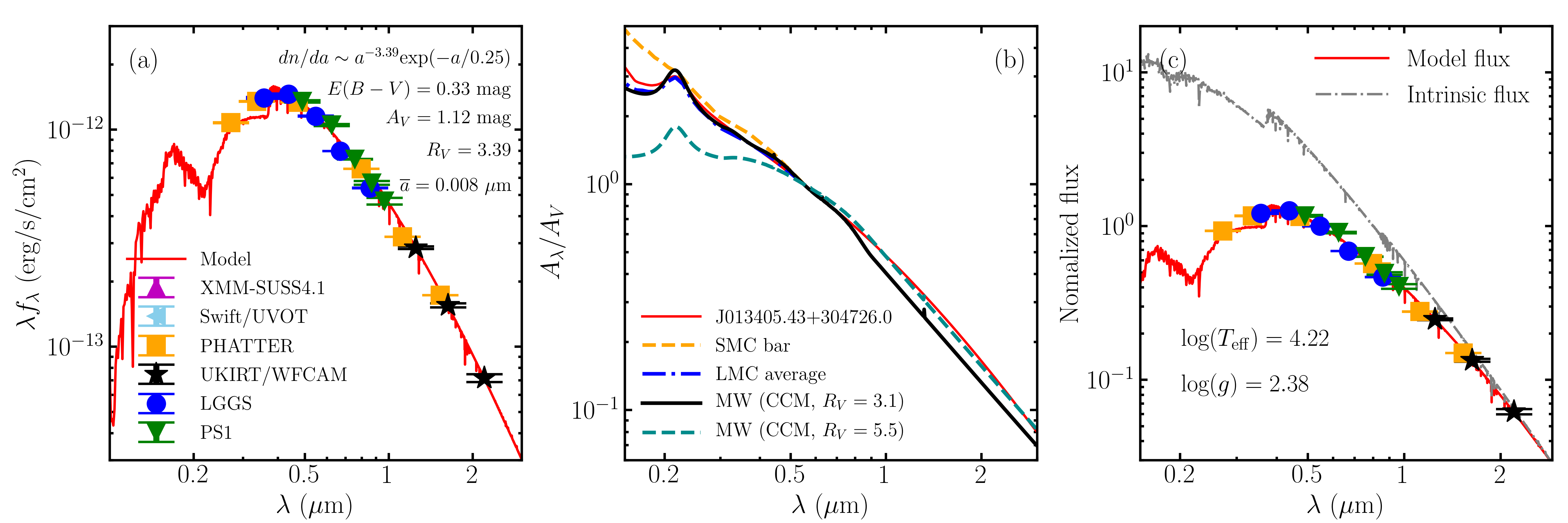
With the model SEDs fit to the observed data, the fitting parameters for each tracer, including in the dust model, extinction in the band , the effective temperature log and the surface gravity log, can be derived, as well as the corresponding extinction curve, the average dust radius , the color excess , and the total-to-selective extinction ratio . The average dust radius is derived based on equation (8) in Nozawa 2016. is derived by , and then . The results for one star in the extinction sample are plotted in Figure 2 as an example to show the comparison of the best-fitting model SED to the observed data with fitting parameters , , the derived parameters , and marked, the corresponding extinction curve and the comparison of normalized model SED and normalized intrinsic SED.
III.3 Results Screening
As mentioned in 108, pcFlag is also introduced in this work to show the coverage of passbands adopted in the calculation for each tracers and the sample of the extinction tracers in this work is therefore divided into four subsamples (pcFlag = ‘UVI’, pcFlag = ‘UV’, pcFlag = ‘VI’, pcFlag = ‘V’)44 4 U in pcFlag means the results are derived with UV data (here, this refers to the passbands bluer than the band), while V and I in pcFlag are short for visual bands and near-IR bands (here, this refers to the passbands redder than the band), respectively.. The numbers of the tracers in the four subsamples are 58, 20, 73 and 192, respectively. It is considered that the results for the sight lines with pcFlag = ‘UVI’ are the most reliable, which are adopted to analyze the extinction curves in this work. The criteria used to select the reasonable results are similar to those in 108, as follows:
I. The acceptance fraction, which indicates the fraction of proposed steps that are accepted in the MCMC process, is in the range of 0.2 - 0.5 (Foreman-Mackey et al. 2013).
II. The derived color excess is larger than the foreground extinction for M33 [ mag] because slightly reddened stars may lead to larger errors (Clayton et al. 2015).
III. The derived total-to-selective extinction ratio is in the range of . In our extinction sample, there are also some reddened stars with good MCMC performance, yet the derived values of are unusually as high () as those in 108. The results may lead to acceptable models that fit the observations well, but the derived values of are unphysical because the values of are observationally in the range of (Mathis 1990; Welty & Fowler 1992; Fitzpatrick 1999; Draine 2011; Wang et al. 2017).
There are 58 tracers with pcFlag = ‘UVI’ in the extinction sample, of which 39 tracers are selected for the further analysis based on the selection criteria mentioned above. It is anticipated that sufficient data covering UV to near-IR bands will bring more reliable results, because UV and near-IR data can effectively constrain the extinction curve and the intrinsic spectra. Although the results with pcFlag = ‘UVI’ are recommended in this work, we also present the selected results for the tracers from the other three subsamples in the following section (see Table and Table ) as a reference.
IV Results and discussion
IV.1 The Extinction Curves in M33
The results for each selected tracer are partly listed in Table , of which the entirety is available in machine-readable form. The ID and spectral type for each tracer are extracted from the LGGS catalog (Massey et al. 2016). The fitting parameter [, log, log and ] and the uncertainties are derived based on the 50%, 16% and 84% values of the parameter spaces generated from the EMCEE results. The corresponding values of , and derived in Section III.2 are also listed in Table . The columns named “Total bands” and “pcFlag” in Table present the number of passbands and the coverage of the passbands adopted in the calculation. The columns following the “pcFlag” column are the photometric information in each band, which are available in a machine-readable format. It should be noted that although extinction curves with smaller values usually have stronger 2175 bumps and steeper far-UV rises, the CCM extinction law with only one parameter is not generally applied in external galaxies (Clayton et al. 2015); thus, cannot completely describe the extinction features on the extinction curves in external galaxies (108). As a result, we prefer to adopt the parameter in the dust size distribution function to describe the dust extinction and dust properties in M33 in this work.
Table summarizes the median values with the upper and lower limits of each parameter. As mentioned in Section III.3, we divide our extinction sample into four subsamples based on the coverage of passbands adopted in the calculation (pcFlag). Lines 1 to 4 in Table present the results of the four subsamples, and the fifth line shows the results of all the selected tracers in the extinction sample. As illustrated in 108, the results for the sight lines with pcFlag = ‘UVI’ are the most reliable and are consequently adopted to describe the general extinction law in M33. Lines 6 to 9 in Table show the influence of the lack of UV or near-IR data on the results (see Section IV.4 for details). The last line in Table is the results of fitting our model extinction curves derived directly from the silicate-graphite dust model to the MW extinction curve (Fitzpatrick et al. 2019, 32 hereafter) for comparison.
The extinction curves toward the sight lines with pcFlag = ‘UVI’ are plotted in Figure 3 with gray solid lines. The extinction curves in M33 cover a wide range of shapes, from flat extinction curves with large to steep curves with obvious 2175 bumps, indicating the inhomogeneous interstellar environment and dust distribution in M33. The red solid line in Figure 3 shows the average extinction derived based on the median value of the fitting parameter for the sight lines with pcFlag = ‘UVI’. The average extinction curve in M33 shows similarity to the extinction curve in the diffuse region of the MW and the average LMC extinction curve, but with a slightly weaker 2175 bump and a slightly steeper rise in the UV bands. The average extinction law in M33 derived in this work can be applied to the general extinction correction in M33, and those toward individual sight lines can help with high-precision extinction correction (see Section IV.5 for details).
The dust size distributions toward the selected tracers with pcFlag = ‘UVI’ are plotted in Figure 4 with gray solid lines. As we know, grains with sizes that are comparable to the wavelength absorb and scatter light most effectively (, where a is the spherical radius of the grain, Li 2009). Interstellar dust has long been considered to be “submicron-sized” () since dust extinction was first confirmed by Trumpler 1930, because grain models that reproduce the observed extinction should have extinction in the visible bands () dominated by grains with (Draine 2011). However, it is now well recognized that the dust size actually spans a wide range from subnanometers to micrometers (Wang et al. 2015). In addition, the strong rise to on the extinction curves requires a large abundance of grain with ; thus, interstellar dust must include a large population of grains with . Based on equation (8) in Nozawa 2016, we derive that the average dust size toward individual sight lines with pcFlag = ‘UVI’ is in the range of 5.78-9.64 nm. The median value of the average dust size is nm, which is smaller than those of the MW ( nm) and M31 ( nm).
=1.5in {rotatetable}
| J013244.40+301547.7 | B6I | 7.53 | 0.23 | 3.24 | 11 | UVI | ||||
| J013250.65+304005.3 | B3I | 8.89 | 0.07 | 5.01 | 5 | V | ||||
| J013256.37+303552.1 | B1Ia | 8.51 | 0.08 | 4.53 | 16 | UVI | ||||
| J013256.61+302740.6 | B1.5Ia+Neb | 7.69 | 0.10 | 3.46 | 10 | V | ||||
| J013307.49+303042.7 | B7I | 6.46 | 0.13 | 1.93 | 16 | UVI |
Note. — a This is an extracted table, and the entire table is available in machine-readable form.
b The dust size distribution can be expressed as follows: , as described in Section III.
c The final results and the uncertainties for each parameter are derived from the 50th, 16th and 84th percentiles of the parameter spaces from the EMCEE results.
d The average dust radius is calculated from equation (8) in Nozawa 2016.
e This is the flag for the coverage of passbands adopted in the calculation. U = UV bands (here, this refers to the passbands bluer than the band). V = Visual band (here, this refers to the passbands from the to bands). I = IR band (here, this refers to the passbands redder than the band).
| pcFlag = ‘UVI’b | 39 | |||||
|---|---|---|---|---|---|---|
| pcFlag = ‘UV’ | 14 | |||||
| pcFlag = ‘VI’ | 32 | |||||
| pcFlag = ‘V’ | 41 | |||||
| All tracers | 126 | |||||
| Tracers with near-IR datac | 71 | |||||
| 51d | ∗ | ∗ | ∗ | ∗ | ∗ | |
| Tracers with UV datac | 53 | |||||
| 36d | ∗ | ∗ | ∗ | ∗ | ∗ | |
| MW (F19, )e | 3.37 | 8.36 |
Note. — a The superscript and the subscript in the table indicate the derived upper limit value and lower value of the derived parameters extracted from Table for the selected tracers.
b The results of the sight lines with pcFlag = ‘UVI’ are adopted to derive the general extinction law in M33.
c For tracers with near-IR (UV) data, the calculation is repeated without taking near-IR (UV) data into consideration, and reliable results are listed with ∗ for comparison.
d For the 71 (53) tracers with near-IR (UV) data, when repeating the calculation without adopting near-IR (UV) data, reliable results can be derived for only 51 (36) tracers.
e The Levenberg-Marquardt method is adopted to fit the model extinction curves to the F19 extinction curve with . There is only one parameter () in our model extinction curves, and a grid ranging from 0.50 to 7.00 with a step of 0.01 is taken.


IV.2 Comparison with the Local Galaxies
We compare the average extinction curve in M33 with those in the MW and other local group galaxies (SMC, LMC, M31) in Figure 3. The average LMC extinction law (Nandy & Morgan 1978; Fitzpatrick 1986; Gordon et al. 2003) resembles that in the MW, while most of the extinction curves in the SMC bar region (Prevot et al. 1984; Gordon et al. 2003) display a nearly linear rise with and an absent 2175 , similar to those in the starburst galaxies (Calzetti et al. 1994). The average extinction curve in M31 derived in 108 (yellow dashed lines in Figure 3) shows similarity to that of the MW but rises less steeply in the far-UV bands. The average extinction curve in M33 is similar to that of M31 in shape but with a slightly larger slope.
The average dust extinction curve derived in this work is also compared with the attenuation curves derived in Gordon et al. 1999 and Hagen 2017 in Figure 3. As illustrated in Section I, attenuation curves include both extinction and the assumed geometry of dust and stars, so attenuation is aimed at the effect of dust on an area instead of an individual sight line. Gordon et al. 1999 adopted radiative transfer modeling from UV to NIR of the M33 nucleus, which is an ideal interstellar environment of starburst, and found an MW-like attenuation curve with a strong 2175 bump (solid cyan line in Figure 3). Hagen 2017 modeled the SEDs for 1170 large pixels in M33 from FUV to NIR and derived a steep median attenuation curve with a weaker 2175 bump (solid green line in Figure 3).
The average extinction curve in M33 derived in this work presents a similar slope to Gordon et al. 1999 but with a weaker 2175 bump as the median one in Hagen 2017. In this work, we map the derived of the selected tracers in Figure 5 and find that the median value of is 0.43 mag, which is slightly smaller than the median ( mag) derived in (Hagen 2017) and larger than the mean amount of dust extinction ( mag) measured in Verley et al. 2009. The discrepancy may be due to the different scales of dust and the different stellar models (Conroy 2013). In addition, we eliminate the results with mag, as mentioned in Section III.3, because slightly reddened stars may lead to larger errors. As a result, tracers with small values are excluded, increasing the median value of .
Moeller & Calzetti 2022 combined the Starburst99 (Leitherer et al. 1999)+YGGDRASIL (Zachrisson et al. 2011) simple stellar population models and the starburst attenuation curve (Calzetti et al. 2000) to model the SEDs of the young star cluster population in M33. They found that all the star clusters have moderate-to-small internal extinction, i.e., all the star clusters have mag and approximately 2/3 of them have mag. We also derive small extinction values for all the supergiants in our extinction sample, i.e., all the supergiants have mag, and approximately 2/3 of them have mag, which is consistent with Moeller & Calzetti 2022.

IV.3 The 2175 bump
The 2175 bump, which is the broad excess in the extinction curve at a rest wavelength , is the strongest signature of dust in the interstellar medium (Kashino et al. 2021). It has been considered as a unique probe of the nature of dust in galaxies since it was discovered by Stecher 1965. The 2175 bump is obvious in the extinction curves toward the individual sight lines of the MW (e.g., Fitzpatrick & Massa 1986; Fitzpatrick & Massa 1990; 32), LMC (Nandy & Morgan 1978; Fitzpatrick 1986; Gordon et al. 2003) and M31 (Dong et al. 2014; Clayton et al. 2015; 108), while it was almost absent in the SMC (Prevot et al. 1984; Gordon et al. 2003). On galaxy scales, it was found that there is no significant 2175 bump in the attenuation curves of nearby starburst galaxies (Calzetti et al. 1994; Gordon et al. 1997; Calzetti et al. 2000) and Lyman break galaxies at high redshifts (, Vijh et al. 2003). As a result, the attenuation curves with no 2175 bump in Calzetti et al. 2000 are commonly adopted for both local and distant star-forming galaxies. However, the 2175 bump has been detected and even measured for star-forming galaixes by many recent works (e.g. Noll et al. 2007; Noll et al. 2009; Buat et al. 2011; Buat et al. 2012; Scoville et al. 2015; Battisti et al. 2017; Salim et al. 2018; Battisti et al. 2020; Shivaei et al. 2020).
As to M33, although it was one of the star-forming galaxies in Calzetti et al. 1994 with no significant 2175 bump in the attenuation curve, recent studies (Gordon et al. 1999; Hagen 2017) indicated that there exists a 2175 bump in the attenuation curve. Since graphite is one of the possible candidates of the carriers of the 2175 bump (Stecher & Donn 1965), we adopt the silicate-graphite dust model in this work to derive the overall extinction curves from UV to near-IR toward individual sight lines in M33. In order to find out whether the 2175 bump really exists in the extinction curves of M33, we also adopt the model extinction curves without a 2175 bump derived from the silicate dust model (, no carbonaceous grains) to repeat the calculation for the tracers with ultraviolet data. By comparing the median values of 55 5 , where is the number of the observed photometric points adopted in the calculation, is the number of adjustable parameters (see Section III.1 for details), is the observed flux of the photometric point, is the model flux of the photometric point and is the difference between logarithm of extreme and logarithm of . derived from both dust models for each tracer, it is found that the extinction curves derived from the silicate-graphite dust model can generally recover the observed SEDs better than the silicate dust model. We therefore suggest that there exists a 2175 bump in the extinction curves of M33. The fine structure of the UV extinction curves can be analyzed and more comprehensive results can be expected, if the UV data is adequate in the future.
IV.4 Influence of IR and UV Photometry
Photometric data that cover a wider range of passbands will constrain the observed SED better and bring more reliable results. Because of the observation limit, a number of tracers lack photometry in the and PHATTER bands. Meanwhile, UKIRT data are also not applied to all tracers in the extinction sample, as mentioned in Section II. It is thus necessary to determine whether the lack of photometry in the UV and near-IR bands affects the derived extinction law.
Lines 6 and 8 in Table summarize the results of the selected tracers with near-IR data and with UV data, respectively. We repeat the calculation for these two groups of tracers but ignore the near-IR data or UV data and list the number of tracers with reliable results as well as the derived results in the seventh and ninth lines of Table , respectively. As shown in Table , the number of tracers with reliable results is significantly reduced when UV data or near-IR data are not adopted in the calculation, indicating that photometric data in wider bands bring more reliable results.
On the other hand, we compare the reliable results derived with near-IR (UV) data ignored for the tracers with near-IR (UV) data [Tracers in Line 6 (8) of Table ] and the results extracted from Table for the same tracers in Figure 6. As Figure 6 shows, the lack of UV or near-IR data has little impact on and in this work. However, the dust size parameter and the average dust size for most of the individual tracers are influenced by the coverage of the adopted passbands, indicating that UV and near-IR data are important to constrain the dust model.
To illustrate the reliability of the derived results for individual sight lines, as mentioned in Section II, we introduce pcFlag in Table to show the coverage of passbands adopted in the calculation. The results of sight lines with pcFlag = ‘UVI’ are the most reliable, while those with pcFlag = ‘V’ are the least reliable. We anticipate that the results could be more comprehensive if the observed data in multiple bands are adequate, especially in UV bands, because UV data can provide a strong constraint on the extinction model. The coming 2 m-aperture Survey Space Telescope (also known as the China Space Station Telescope, CSST) will image approximately 17500 square degrees of the sky in the , , , , , and bands (Zhan 2021) and will provide us with abundant data to explore the dust extinction law in M33 and other nearby star-resolved galaxies.

IV.5 Prediction of Multiband Extinction
As mentioned in Section IV.1, the dust extinction curves derived in this work can help with the extinction correction in M33. Based on the average extinction curve of M33 in this work, multiband extinction values from UV to near-IR are predicted, which are shown in Table . High-precision extinction correction should refer to the extinction law of individual tracers derived in this work. Table partially lists the extinction values in multiple bands from UV to near-IR toward individual sight lines, and the entire table is available in machine-readable form. The ID, spectral type, right ascension and declination listed in the first four columns of Table for each tracer are obtained from the LGGS catalog (Massey et al. 2016). The , and in Table are extracted from Table . The column named pcFlag presents the passband coverage, as shown in Table . The following columns show the extinction values in multiple bands for each tracer. Although the results for some tracers are not affected by the lack of UV or near-IR data, we recommend multiband extinction toward individual sight lines with pcFlag = ‘UVI’.
When applying the method and results in this work, there are three aspects that need to be noted. First, the extinction curves derived in this work are applicable from UV to near-IR () bands. All dust models for the diffuse ISM predict that an extinction curve steeply declines with at and increases at because of the silicate absorption feature (Mathis et al. 1977; Kim et al. 1994; Weingartner & Draine 2001; Li et al. 2015). However, many recent observations suggest that the extinction law in the mid-IR band () appears to be universally flat or gray in various interstellar environments (Lutz et al. 1996; Lutz 1999; Indebetouw et al. 2005; Flaherty et al. 2007; Gao et al. 2009; Nishiyama et al. 2009; Fritz et al. 2011; Wang et al. 2013). Although the -sized grain can be adopted to model the flat mid-IR extinction curve (Wang et al. 2015), it will make the model more complex and, thus, reduce the universality of the method. As a result, the derived extinction curves cannot be applied to mid-IR bands at present.
Moreover, the classic silicate-graphite dust model adopted in this work may not be applied to analyze the fine structure of the extinction curves in UV bands, although it can be adopted to derive the overall reliable extinction curves in M33 from UV to near-IR bands. As illustrated in Section IV.3, the 2175 bump is known to be an important feature of the extinction curves in UV bands, which was first discovered by Stecher 1965. Since Stecher & Donn 1965 pointed out that small graphite particles would produce absorption very similar to this observed feature, some form of graphitic carbon has been an attractive candidate because the transition in graphite is responsible for the absorption feature at (Draine 2003). However, this graphite hypothesis does not appear to explain the fact that the full width at half maxima (FWHM) of 2175 varies with the interstellar environment while holding the central wavelength nearly constant (Draine & Malhotra 1993). Currently, a polycyclic aromatic hydrocarbon (PAH) mixtures are carrier candidates for the 2175 bump (Joblin et al. 1992; Li & Draine 2001; Xiang et al. 2011; Steglich et al. 2011; Mishra & Li 2015; Mishra & Li 2017) because PAH molecules generally have strong absorption in the 2000 - 2500 region with variation in FWHM and small variation in . As a result, we consider adding PAHs to the dust model in future work to analyze the fine structure of UV extinction curves and obtain a more detailed understanding of the dust properties in M33 and other nearby galaxies.
Finally, as shown in Figure 5, the size of the extinction sample adopted in this work is not adequate to cover the entire region of M33. Thus, it can only provide us with a low-resolution extinction map to help with a rough extinction correction for certain regions in M33. A major science project named CSST mentioned in Section IV.4 will provide us with larger extinction samples and adequate data in multiple bands. We can expect further exploration of the dust properties and extinction law in M33 and in other nearby star-resolved galaxies, as well as the development of higher-precision extinction corrections in the near future.
| /UVOT | 0.209 | ||
|---|---|---|---|
| /UVOT | 0.225 | ||
| /UVOT | 0.268 | ||
| /PHAT | 0.272 | ||
| /CSST | 0.29 | ||
| /PHAT | 0.336 | ||
| 0.357 | |||
| 0.443 | |||
| /PHAT | 0.473 | ||
| /CSST | 0.475 | ||
| 0.554 | |||
| /CSST | 0.612 | ||
| 0.67 | |||
| /CSST | 0.758 | ||
| /PHAT | 0.798 | ||
| 0.857 | |||
| /CSST | 0.911 | ||
| /CSST | 0.989 | ||
| /PHAT | 1.12 | ||
| /2MASS | 1.235 | ||
| /PHAT | 1.528 | ||
| /2MASS | 1.662 | ||
| /2MASS | 2.159 |
Note. — a For the effective wavelengths of multiple bands (except CSST bands) used in this work refer to the SVO Filter Profile Service (http://svo2.cab.inta-csic.es/theory/fps/, Rodrigo et al. 2012). The effective wavelengths of the CSST bands are calculated by , where is the filter transmission function and is the Vega spectrum.
b is the average extinction in M33 based on the median value of .
= 2in {rotatetable}
| J013244.40+301547.7 | B6I | 01 32 44.37 | +30 15 47.6 | 3.46 | 7.53 | 0.23 | UVI | 0.76 | 8.37 | 7.3 | 3.23 | 3.08 |
| J013250.65+304005.3 | B3I | 01 32 50.62 | +30 40 05.2 | 2.93 | 8.89 | 0.07 | V | 0.37 | 4.1 | 3.58 | 1.58 | 1.51 |
| J013256.37+303552.1 | B1Ia | 01 32 56.34 | +30 35 52.0 | 3.04 | 8.51 | 0.08 | UVI | 0.35 | 3.9 | 3.41 | 1.51 | 1.44 |
| J013256.61+302740.6 | B1.5Ia+Neb | 01 32 56.58 | +30 27 40.5 | 3.37 | 7.69 | 0.1 | V | 0.35 | 3.87 | 3.38 | 1.49 | 1.43 |
| J013307.49+303042.7 | B7I | 01 33 07.46 | +30 30 42.6 | 4.35 | 6.46 | 0.13 | UVI | 0.26 | 1.2 | 1.14 | 0.72 | 0.7 |
Note. — a This is an extracted table for the same tracers as listed in Table with a portion of the multiband extinction values. The entire table is available in machine-readable form.
b Flag for the coverage of passbands adopted in the calculation (the same as Table )
IV.6 Application in Other Nearby Star-Resolved Galaxies
The method adopted in this work and 108 is extended to other nearby star-resolved galaxies. The LGGS provides plus the interference-image photometry of luminous stars in seven systems currently forming massive stars (IC 10, NGC 6822, WLM, Sextans A and B, Pegasus and Phoenix, Massey et al. 2007) in addition to the spiral galaxies M31 and M33 (Massey et al. 2006; Massey et al. 2016). We can isolate O-type and B-type supergiants in NGC 6822 and WLM from the LGGS catalog (Massey et al. 2007), which are selected as the extinction tracers.
The observed data for the tracers in NGC 6822 and WLM are from the LGGS catalog (Massey et al. 2007), the PS1 survey (Chambers et al. 2016), the UKIRT (Irwin 2013) and the HST (Bianchi et al. 2017, only for NGC 6822). We adopt mag and mag to remove the foreground extinction for NGC 6822 and WLM (Schlafly & Finkbeiner 2011), respectively. The process for constructing the model SEDs for the tracers is the same as mentioned in Section III.1, but we adopt for both NGC 6822 and WLM (Leaman 2012; Ren et al. 2021a; Ren et al. 2021b). After result selection with the criteria mentioned in Section III.366 6 Instead of mag, we consider the foreground extinction values for NGC 6822 and WLM as the second selection criterion listed in Section III.3., 6 tracers in NGC 6822 and 4 tracers in WLM with reliable results are selected for further analysis.
The results for all the selected tracers are listed in Table , and the derived extinction curves in NGC 6822 and WLM are plotted in Figure 7 (a) and (b), respectively, and compared with those in WM (F19, , black dashed line), M31 (108, yellow dashed line) and M33 (this work, cyan dashed line). There is only one extinction curve in NGC 6822 toward the sight line with pcFlag = ‘UVI’, which shows a steeper far-UV rise than the average ones in the MW, M31 and M33, indicating a smaller dust size. The average extinction curves presented in Figure 7 are calculated from the median values of derived for the selected traces, which can only represent the average results in this work rather than the whole galaxies. More photometric data in various bands are needed to obtain a better understanding of the extinction law and the dust properties in NGC 6822, WLM and other nearby star-resolved galaxies.

= 1.5in {rotatetable}
| NGC 6822 | J194451.18-144919.8 | B0-1Ia | 7.93 | 0.30 | 3.77 | 10 | V | ||||
| NGC 6822 | J194455.47-144930.0 | B1-2I | 6.93 | 0.29 | 2.52 | 5 | V | ||||
| NGC 6822 | J194450.21-144253.6 | B1.5I | 6.89 | 0.26 | 2.48 | 5 | V | ||||
| NGC 6822 | J194452.28-145220.6 | B1I | 6.77 | 0.40 | 2.35 | 8 | VI | ||||
| NGC 6822 | J194455.08-145213.1 | B5Ia | 5.83 | 0.65 | 1.96 | 4 | V | ||||
| NGC 6822 | J194501.60-145440.0 | B8-A0:I | 7.26 | 0.28 | 2.91 | 9 | UVI | ||||
| NGC 6822 | Averageb | - | 3.88 | - | - | 0.89 | 6.91 | 0.30 | 2.50 | - | - |
| WLM | J000157.20-152718.0 | B1.5Ia | 6.64 | 0.21 | 2.21 | 5 | V | ||||
| WLM | J000158.12-152648.5 | B1.5Ia | 6.92 | 0.10 | 2.52 | 5 | V | ||||
| WLM | J000153.22-152839.5 | B9Ia | 8.56 | 0.10 | 4.57 | 12 | VI | ||||
| WLM | J000159.95-152819.0 | O9.7Ia | 6.00 | 0.13 | 1.90 | 12 | VI | ||||
| WLM | Averageb | - | 4.00 | - | - | 0.35 | 6.78 | 0.12 | 2.37 | - | - |
Note. — a The columns descriptions are the same as those for Table .
b These lines show the median values of the derived parameters for selected tracers in NGC 6822 and WLM.
V Summary
A sample of bright O-type and B-type supergiants from the LGGS catalog (Massey et al. 2016) are chosen as extinction tracers to derive the dust extinction curves in M33. This is the first study focused on the dust extinction curves toward individual sight lines in M33 rather than the dust attenuation curves in Gordon et al. 1999; Hagen 2017. The previous studies have been improved, and the main results of this work are as follows:
1. The extinction curves in M33 derived in this work cover a wide range of shapes, from curves with an obvious 2175 bump (like the extinction curves with ) to relatively flat curves with , implying the complexity of the interstellar environment and the inhomogeneous distribution of interstellar dust in M33. The derived parameter in the dust size distribution ranges from , while the dust size ranges from nm.
2. The average extinction curve in M33 () is similar to the MW extinction curve with but with a slightly weaker 2175 bump and a slightly steeper far-UV rise. The average dust size distribution in M33 is , and the median value of the average dust size is nm, which is smaller than that of the MW ( nm).
3. The derived in M33 is up to 2 mag with a median value of mag, which is smaller than the median value ( mag) derived in Hagen 2017 and larger than the mean amount ( mag) measured by Verley et al. 2009.
4. The method adopted in this work and 108 that combines the stellar model atmospheres and the dust models to calculate extinction curves and analyze dust properties toward individual sight lines is extended to the star-resolved galaxies NGC 6822 and WLM, but we can only derive the extinction curves toward a few individual sight lines. More observations are needed to gain a better understanding of the extinction law and dust properties in nearby star-resolved galaxies.
References
- Asplund et al. (2009) Asplund, M., Grevesse, N., Sauval, A. J., & Scott, P. 2009, ARA&A, 47, 481, doi: 10.1146/annurev.astro.46.060407.145222
- Battisti et al. (2017) Battisti, A. J., Calzetti, D., & Chary, R. R. 2017, ApJ, 851, 90, doi: 10.3847/1538-4357/aa9a43
- Battisti et al. (2020) Battisti, A. J., Cunha, E. d., Shivaei, I., & Calzetti, D. 2020, ApJ, 888, 108, doi: 10.3847/1538-4357/ab5fdd
- Bianchi (2009) Bianchi, L. 2009, Ap&SS, 320, 11, doi: 10.1007/s10509-008-9761-3
- Bianchi et al. (1996) Bianchi, L., Clayton, G. C., Bohlin, R. C., Hutchings, J. B., & Massey, P. 1996, ApJ, 471, 203, doi: 10.1086/177963
- Bianchi et al. (2017) Bianchi, L., Shiao, B., & Thilker, D. 2017, ApJS, 230, 24, doi: 10.3847/1538-4365/aa7053
- Bless & Savage (1970) Bless, R. C., & Savage, B. D. 1970, in IAU Symposium, Vol. 36, Ultraviolet Stellar Spectra and Related Ground-Based Observations, ed. R. Muller, L. Houziaux, & H. E. Butler, 28
- Buat et al. (2011) Buat, V., Giovannoli, E., Heinis, S., et al. 2011, A&A, 533, A93, doi: 10.1051/0004-6361/201117264
- Buat et al. (2012) Buat, V., Noll, S., Burgarella, D., et al. 2012, A&A, 545, A141, doi: 10.1051/0004-6361/201219405
- Calzetti et al. (2000) Calzetti, D., Armus, L., Bohlin, R. C., et al. 2000, ApJ, 533, 682, doi: 10.1086/308692
- Calzetti et al. (1994) Calzetti, D., Kinney, A. L., & Storchi-Bergmann, T. 1994, ApJ, 429, 582, doi: 10.1086/174346
- Cardelli et al. (1989) Cardelli, J. A., Clayton, G. C., & Mathis, J. S. 1989, ApJ, 345, 245, doi: 10.1086/167900
- Castelli & Kurucz (2003) Castelli, F., & Kurucz, R. L. 2003, in Modelling of Stellar Atmospheres, ed. N. Piskunov, W. W. Weiss, & D. F. Gray, Vol. 210, A20. https://arxiv.org/abs/astro-ph/0405087
- Chambers et al. (2016) Chambers, K. C., Magnier, E. A., Metcalfe, N., et al. 2016, arXiv e-prints, arXiv:1612.05560. https://arxiv.org/abs/1612.05560
- Clayton et al. (2015) Clayton, G. C., Gordon, K. D., Bianchi, L. C., et al. 2015, ApJ, 815, 14, doi: 10.1088/0004-637X/815/1/14
- Clayton & Martin (1985) Clayton, G. C., & Martin, P. G. 1985, ApJ, 288, 558, doi: 10.1086/162821
- Conroy (2013) Conroy, C. 2013, ARA&A, 51, 393, doi: 10.1146/annurev-astro-082812-141017
- Conti et al. (2008) Conti, P. S., Crowther, P. A., & Leitherer, C. 2008, From Luminous Hot Stars to Starburst Galaxies
- Cox (2000) Cox, A. N. 2000, Allen’s astrophysical quantities
- Dong et al. (2014) Dong, H., Li, Z., Wang, Q. D., et al. 2014, ApJ, 785, 136, doi: 10.1088/0004-637X/785/2/136
- Draine (2003) Draine, B. T. 2003, ARA&A, 41, 241, doi: 10.1146/annurev.astro.41.011802.094840
- Draine (2011) —. 2011, Physics of the Interstellar and Intergalactic Medium
- Draine & Malhotra (1993) Draine, B. T., & Malhotra, S. 1993, ApJ, 414, 632, doi: 10.1086/173109
- Draine et al. (2014) Draine, B. T., Aniano, G., Krause, O., et al. 2014, ApJ, 780, 172, doi: 10.1088/0004-637X/780/2/172
- Fitzpatrick (1986) Fitzpatrick, E. L. 1986, AJ, 92, 1068, doi: 10.1086/114237
- Fitzpatrick (1999) —. 1999, PASP, 111, 63, doi: 10.1086/316293
- Fitzpatrick (2004) Fitzpatrick, E. L. 2004, in Astronomical Society of the Pacific Conference Series, Vol. 309, Astrophysics of Dust, ed. A. N. Witt, G. C. Clayton, & B. T. Draine, 33. https://arxiv.org/abs/astro-ph/0401344
- Fitzpatrick & Massa (1986) Fitzpatrick, E. L., & Massa, D. 1986, ApJ, 307, 286, doi: 10.1086/164415
- Fitzpatrick & Massa (1990) —. 1990, ApJS, 72, 163, doi: 10.1086/191413
- Fitzpatrick & Massa (2005) —. 2005, AJ, 130, 1127, doi: 10.1086/431900
- Fitzpatrick & Massa (2007) —. 2007, ApJ, 663, 320, doi: 10.1086/518158
- Fitzpatrick et al. (2019) Fitzpatrick, E. L., Massa, D., Gordon, K. D., Bohlin, R., & Clayton, G. C. 2019, ApJ, 886, 108, doi: 10.3847/1538-4357/ab4c3a
- Flaherty et al. (2007) Flaherty, K. M., Pipher, J. L., Megeath, S. T., et al. 2007, ApJ, 663, 1069, doi: 10.1086/518411
- Foreman-Mackey et al. (2013) Foreman-Mackey, D., Hogg, D. W., Lang, D., & Goodman, J. 2013, PASP, 125, 306, doi: 10.1086/670067
- Freedman et al. (1991) Freedman, W. L., Wilson, C. D., & Madore, B. F. 1991, ApJ, 372, 455, doi: 10.1086/169991
- Fritz et al. (2011) Fritz, T. K., Gillessen, S., Dodds-Eden, K., et al. 2011, ApJ, 737, 73, doi: 10.1088/0004-637X/737/2/73
- Galliano et al. (2018) Galliano, F., Galametz, M., & Jones, A. P. 2018, ARA&A, 56, 673, doi: 10.1146/annurev-astro-081817-051900
- Gao et al. (2009) Gao, J., Jiang, B. W., & Li, A. 2009, ApJ, 707, 89, doi: 10.1088/0004-637X/707/1/89
- Gao et al. (2015) Gao, J., Jiang, B. W., Li, A., Li, J., & Wang, X. 2015, ApJ, 807, L26, doi: 10.1088/2041-8205/807/2/L26
- Gao et al. (2013) Gao, J., Li, A., & Jiang, B. W. 2013, Earth, Planets, and Space, 65, 1127, doi: 10.5047/eps.2013.05.016
- Gao et al. (2020) Gao, W., Zhao, R., Gao, J., Jiang, B., & Li, J. 2020, Planet. Space Sci., 183, 104627, doi: 10.1016/j.pss.2018.12.010
- Gordon et al. (1997) Gordon, K. D., Calzetti, D., & Witt, A. N. 1997, ApJ, 487, 625, doi: 10.1086/304654
- Gordon et al. (2003) Gordon, K. D., Clayton, G. C., Misselt, K. A., Land olt, A. U., & Wolff, M. J. 2003, ApJ, 594, 279, doi: 10.1086/376774
- Gordon et al. (1999) Gordon, K. D., Hanson, M. M., Clayton, G. C., Rieke, G. H., & Misselt, K. A. 1999, ApJ, 519, 165, doi: 10.1086/307350
- Hagen (2017) Hagen, L. M. Z. 2017, PhD thesis, The Pennsylvania State University
- Hubeny & Lanz (2017a) Hubeny, I., & Lanz, T. 2017a, arXiv e-prints, arXiv:1706.01859. https://arxiv.org/abs/1706.01859
- Hubeny & Lanz (2017b) —. 2017b, arXiv e-prints, arXiv:1706.01937. https://arxiv.org/abs/1706.01937
- Hubeny & Lanz (2017c) —. 2017c, arXiv e-prints, arXiv:1706.01935. https://arxiv.org/abs/1706.01935
- Indebetouw et al. (2005) Indebetouw, R., Mathis, J. S., Babler, B. L., et al. 2005, ApJ, 619, 931, doi: 10.1086/426679
- Irwin (2013) Irwin, M. J. 2013, in Thirty Years of Astronomical Discovery with UKIRT, Vol. 37, 229, doi: 10.1007/978-94-007-7432-2_21
- Joblin et al. (1992) Joblin, C., Leger, A., & Martin, P. 1992, ApJ, 393, L79, doi: 10.1086/186456
- Kashino et al. (2021) Kashino, D., Lilly, S. J., Silverman, J. D., et al. 2021, ApJ, 909, 213, doi: 10.3847/1538-4357/abdf62
- Kim et al. (1994) Kim, S.-H., Martin, P. G., & Hendry, P. D. 1994, ApJ, 422, 164, doi: 10.1086/173714
- Leaman (2012) Leaman, R. 2012, AJ, 144, 183, doi: 10.1088/0004-6256/144/6/183
- Leitherer et al. (1999) Leitherer, C., Schaerer, D., Goldader, J. D., et al. 1999, ApJS, 123, 3, doi: 10.1086/313233
- Lequeux et al. (1982) Lequeux, J., Maurice, E., Prevot-Burnichon, M. L., Prevot, L., & Rocca-Volmerange, B. 1982, A&A, 113, L15
- Li & Draine (2001) Li, A., & Draine, B. T. 2001, ApJ, 554, 778, doi: 10.1086/323147
- Li et al. (2015) Li, A., Wang, S., Gao, J., & Jiang, B. W. 2015, Dust in the Local Group, 85, doi: 10.1007/978-3-319-10614-4_8
- Li (2009) Li, H. 2009, Smart Hydrogel Modelling, doi: 10.1007/978-3-642-02368-2
- Liu et al. (2019) Liu, Z., Cui, W., Liu, C., et al. 2019, ApJS, 241, 32, doi: 10.3847/1538-4365/ab0a0d
- Lutz (1999) Lutz, D. 1999, in ESA Special Publication, Vol. 427, The Universe as Seen by ISO, ed. P. Cox & M. Kessler, 623
- Lutz et al. (1996) Lutz, D., Feuchtgruber, H., Genzel, R., et al. 1996, A&A, 315, L269
- Magrini et al. (2007a) Magrini, L., Corbelli, E., & Galli, D. 2007a, A&A, 470, 843, doi: 10.1051/0004-6361:20077215
- Magrini et al. (2007b) Magrini, L., Vílchez, J. M., Mampaso, A., Corradi, R. L. M., & Leisy, P. 2007b, A&A, 470, 865, doi: 10.1051/0004-6361:20077445
- Martin et al. (2005) Martin, D. C., Fanson, J., Schiminovich, D., et al. 2005, ApJ, 619, L1, doi: 10.1086/426387
- Massey et al. (2016) Massey, P., Neugent, K. F., & Smart, B. M. 2016, AJ, 152, 62, doi: 10.3847/0004-6256/152/3/62
- Massey et al. (2007) Massey, P., Olsen, K. A. G., Hodge, P. W., et al. 2007, AJ, 133, 2393, doi: 10.1086/513319
- Massey et al. (2006) —. 2006, AJ, 131, 2478, doi: 10.1086/503256
- Mathis (1990) Mathis, J. S. 1990, ARA&A, 28, 37, doi: 10.1146/annurev.aa.28.090190.000345
- Mathis et al. (1977) Mathis, J. S., Rumpl, W., & Nordsieck, K. H. 1977, ApJ, 217, 425, doi: 10.1086/155591
- Mishra & Li (2015) Mishra, A., & Li, A. 2015, ApJ, 809, 120, doi: 10.1088/0004-637X/809/2/120
- Mishra & Li (2017) —. 2017, ApJ, 850, 138, doi: 10.3847/1538-4357/aa937a
- Moeller & Calzetti (2022) Moeller, C., & Calzetti, D. 2022, AJ, 163, 16, doi: 10.3847/1538-3881/ac324e
- Morrissey et al. (2007) Morrissey, P., Conrow, T., Barlow, T. A., et al. 2007, ApJS, 173, 682, doi: 10.1086/520512
- Nandy & Morgan (1978) Nandy, K., & Morgan, D. H. 1978, Nature, 276, 478, doi: 10.1038/276478a0
- Neugent (2021) Neugent, K. F. 2021, ApJ, 908, 87, doi: 10.3847/1538-4357/abd47b
- Neugent et al. (2017) Neugent, K. F., Massey, P., Hillier, D. J., & Morrell, N. 2017, ApJ, 841, 20, doi: 10.3847/1538-4357/aa6e51
- Nilson (1973) Nilson, P. 1973, Uppsala general catalogue of galaxies
- Nishiyama et al. (2009) Nishiyama, S., Tamura, M., Hatano, H., et al. 2009, ApJ, 696, 1407, doi: 10.1088/0004-637X/696/2/1407
- Noll et al. (2007) Noll, S., Pierini, D., Pannella, M., & Savaglio, S. 2007, A&A, 472, 455, doi: 10.1051/0004-6361:20077067
- Noll et al. (2009) Noll, S., Pierini, D., Cimatti, A., et al. 2009, A&A, 499, 69, doi: 10.1051/0004-6361/200811526
- Nozawa (2016) Nozawa, T. 2016, Planet. Space Sci., 133, 36, doi: 10.1016/j.pss.2016.08.006
- Page et al. (2019) Page, M. J., Brindle, C., Talavera, A., et al. 2019, VizieR Online Data Catalog, II/356
- Prevot et al. (1984) Prevot, M. L., Lequeux, J., Maurice, E., Prevot, L., & Rocca-Volmerange, B. 1984, A&A, 132, 389
- Ren et al. (2021a) Ren, Y., Jiang, B., Yang, M., et al. 2021a, ApJ, 907, 18, doi: 10.3847/1538-4357/abcda5
- Ren et al. (2021b) Ren, Y., Jiang, B., Yang, M., Wang, T., & Ren, T. 2021b, arXiv e-prints, arXiv:2110.08793. https://arxiv.org/abs/2110.08793
- Ren et al. (2019) Ren, Y., Jiang, B.-W., Yang, M., & Gao, J. 2019, ApJS, 241, 35, doi: 10.3847/1538-4365/ab0825
- Rodrigo et al. (2012) Rodrigo, C., Solano, E., & Bayo, A. 2012, SVO Filter Profile Service Version 1.0, IVOA Working Draft 15 October 2012, doi: 10.5479/ADS/bib/2012ivoa.rept.1015R
- Ruoyi & Haibo (2020) Ruoyi, Z., & Haibo, Y. 2020, ApJ, 905, L20, doi: 10.3847/2041-8213/abccc4
- Salim et al. (2018) Salim, S., Boquien, M., & Lee, J. C. 2018, ApJ, 859, 11, doi: 10.3847/1538-4357/aabf3c
- Salim & Narayanan (2020) Salim, S., & Narayanan, D. 2020, ARA&A, 58, 529, doi: 10.1146/annurev-astro-032620-021933
- Schlafly & Finkbeiner (2011) Schlafly, E. F., & Finkbeiner, D. P. 2011, ApJ, 737, 103, doi: 10.1088/0004-637X/737/2/103
- Scoville et al. (2015) Scoville, N., Faisst, A., Capak, P., et al. 2015, ApJ, 800, 108, doi: 10.1088/0004-637X/800/2/108
- Shao et al. (2018) Shao, Z., Jiang, B. W., Li, A., et al. 2018, MNRAS, 478, 3467, doi: 10.1093/mnras/sty1267
- Shivaei et al. (2020) Shivaei, I., Reddy, N., Rieke, G., et al. 2020, ApJ, 899, 117, doi: 10.3847/1538-4357/aba35e
- Stecher (1965) Stecher, T. P. 1965, ApJ, 142, 1683, doi: 10.1086/148462
- Stecher & Donn (1965) Stecher, T. P., & Donn, B. 1965, ApJ, 142, 1681, doi: 10.1086/148461
- Steglich et al. (2011) Steglich, M., Bouwman, J., Huisken, F., & Henning, T. 2011, ApJ, 742, 2, doi: 10.1088/0004-637X/742/1/2
- Toribio San Cipriano et al. (2016) Toribio San Cipriano, L., García-Rojas, J., Esteban, C., Bresolin, F., & Peimbert, M. 2016, MNRAS, 458, 1866, doi: 10.1093/mnras/stw397
- Trumpler (1930) Trumpler, R. J. 1930, PASP, 42, 214, doi: 10.1086/124039
- Verley et al. (2009) Verley, S., Corbelli, E., Giovanardi, C., & Hunt, L. K. 2009, A&A, 493, 453, doi: 10.1051/0004-6361:200810566
- Vijh et al. (2003) Vijh, U. P., Witt, A. N., & Gordon, K. D. 2003, ApJ, 587, 533, doi: 10.1086/368344
- Wang & Chen (2019) Wang, S., & Chen, X. 2019, ApJ, 877, 116, doi: 10.3847/1538-4357/ab1c61
- Wang et al. (2013) Wang, S., Gao, J., Jiang, B. W., Li, A., & Chen, Y. 2013, ApJ, 773, 30, doi: 10.1088/0004-637X/773/1/30
- Wang et al. (2017) Wang, S., Jiang, B. W., Zhao, H., Chen, X., & de Grijs, R. 2017, ApJ, 848, 106, doi: 10.3847/1538-4357/aa8db7
- Wang et al. (2014) Wang, S., Li, A., & Jiang, B. W. 2014, Planet. Space Sci., 100, 32, doi: 10.1016/j.pss.2014.03.018
- Wang et al. (2015) —. 2015, ApJ, 811, 38, doi: 10.1088/0004-637X/811/1/38
- Wang et al. (2022) Wang, Y., Gao, J., & Ren, Y. 2022, ApJS, 259, 12, doi: 10.3847/1538-4365/ac3bc6
- Weingartner & Draine (2001) Weingartner, J. C., & Draine, B. T. 2001, ApJ, 548, 296, doi: 10.1086/318651
- Welty & Fowler (1992) Welty, D. E., & Fowler, J. R. 1992, ApJ, 393, 193, doi: 10.1086/171497
- Williams et al. (2014) Williams, B. F., Lang, D., Dalcanton, J. J., et al. 2014, ApJS, 215, 9, doi: 10.1088/0067-0049/215/1/9
- Williams et al. (2021) Williams, B. F., Durbin, M. J., Dalcanton, J. J., et al. 2021, ApJS, 253, 53, doi: 10.3847/1538-4365/abdf4e
- Xiang et al. (2011) Xiang, F. Y., Li, A., & Zhong, J. X. 2011, ApJ, 733, 91, doi: 10.1088/0004-637X/733/2/91
- Yershov (2015) Yershov, V. N. 2015, VizieR Online Data Catalog, II/339
- Zachrisson et al. (2011) Zachrisson, C., Kozachkov, H., Roberts, S., et al. 2011, Journal of Materials Research, 26, 1260, doi: 10.1557/jmr.2011.92
- Zhan (2021) Zhan, H. 2021, Chinese Science Bulletin, , doi: https://doi.org/10.1360/TB-2021-0016