跳到论文正文
W Papers独立论文阅读器 arXiv:2204.05441 论文正文 计算阅读时间 · 0%
引用这篇论文根据当前论文元数据生成,正式投稿前建议核对。


License: arXiv.org perpetual non-exclusive license
arXiv:2204.05441v3 [cond-mat.str-el] 22 Aug 2022

Origin of nonsymmorphic bosonization formulas in generalized antiferromagnetic Kitaev spin-12\frac{1}{2} chains from a renormalization-group perspective

Wang Yang Affiliation: Department of Physics and Astronomy and Stewart Blusson Quantum Matter Institute, University of British Columbia, Vancouver, B.C., Canada, V6T 1Z1    Chao Xu Affiliation: Kavli Institute for Theoretical Sciences, University of Chinese Academy of Sciences, Beijing 100190, China    Alberto Nocera Affiliation: Department of Physics and Astronomy and Stewart Blusson Quantum Matter Institute, University of British Columbia, Vancouver, B.C., Canada, V6T 1Z1    Ian Affleck Affiliation: Department of Physics and Astronomy and Stewart Blusson Quantum Matter Institute, University of British Columbia, Vancouver, B.C., Canada, V6T 1Z1
Abstract

Recently, in the Luttinger liquid phase of the one-dimensional generalized antiferromagnetic Kitaev spin-1/2 model, it has been found that the abelian bosonization formulas of the local spin operators only respect the exact discrete nonsymmorphic symmetry group of the model, not the emergent U(1) symmetry. In this work, we perform a renormalization group (RG) study to provide explanations for the origin of the U(1) breaking terms in the bosonization formulas. We find that the lack of U(1) symmetry originates from the wavefunction renormalization effects in the spin operators along the RG flow induced by the U(1) breaking interactions in the microscopic Hamiltonian. In addition, the RG analysis can give predictions to the signs and order of magnitudes of the coefficients in the bosonization formulas. Our work is helpful to understand the rich nonsymmorphic physics in one-dimensional Kitaev spin models.

I Introduction

Kitaev materials have attracted intense research attentions in the past decade Jackeli2009; Chaloupka2010; Singh2010; Price2012; Singh2012; Plumb2014; Kim2015; Winter2016; Baek2017; Leahy2017; Sears2017; Wolter2017; Zheng2017; Rousochatzakis2017; Kasahara2018; Rau2014; Ran2017; Wang2017; Catuneanu2018; Gohlke2018; Liu2011; Chaloupka2013; Johnson2015; Motome2020, since they not only provide potential experimental platforms for realizing the Kitaev spin-1/2 model on the honeycomb lattice – a prototypical strongly correlated model for topological quantum computations Kitaev2006; Nayak2008, but also are representatives of frustrated magnetic systems, having close relations to the fields of strongly correlated quantum magnetism Fazekas1999; Lauchli2006 and quantum spin liquids Balents2010; Witczak-Krempa2014; Rau2016; Winter2017; Zhou2017; Savary2017. Theoretical and experimental studies have established the fact that Kitaev materials can be described by generalized Kitaev spin models Chaloupka2010; Rau2014; Catuneanu2018; Gohlke2018; Ran2017; Wang2017 which – in addition to Kitaev interaction – contain other types of couplings including the Heisenberg interaction, the off-diagonal Γ\Gamma and Γ′\Gamma^{\prime} terms, and beyond nearest neighbor interactions. One of the central themes in the field of Kitaev materials is to understand the effects of such additional interactions which are inevitable in real materials.

Recently, there has been increasing interests in studying one-dimensional (1D) Kitaev spin models Sela2014; Agrapidis2018; Agrapidis2019; Catuneanu2019; Yang2020; Yang2020a; Yang2020b; Yang2021b; Yang2022; Yang2022b; Luo2021; Luo2021b; You2020; Sorensen2021, which are constructed by selecting one row out of the honeycomb lattice. These 1D Kitaev spin models have discrete nonsymmorphic symmetry group structures Yang2020; Yang2020a; Yang2022, leading to rich physics including emergent conformal symmetries, extended Luttinger liquid phases in the phase diagram, nonvanishing string order parameters, and magnetically ordered phases with exotic symmetry breaking patterns such as Oh→D4O_{h}\rightarrow D_{4} Yang2020; Yang2022b, Oh→D3O_{h}\rightarrow D_{3} Yang2020b; Yang2021b; Yang2022b, Oh→D2O_{h}\rightarrow D_{2} Yang2022b, and D3​d→ℤ2D_{3d}\rightarrow\mathbb{Z}_{2} Yang2020a, where OhO_{h} is the full octahedral group, DnD_{n} is the dihedral group of order 2​n2n, and D3​d≅D3×ℤ2D_{3d}\cong D_{3}\times\mathbb{Z}_{2}. The motivation of such 1D studies is to provide hints and guidance for the 2D physics. Indeed, it has been demonstrated in Ref. Yang2022b that the zigzag phase in 2D Kitaev-Heisenberg-Gamma model can be obtained by weakly coupling an infinite number of 1D chains, thereby providing a controllable approach to the 2D zigzag order. In addition, 1D studies also have their independent merits, since there have been proposals on realizing 1D generalized Kitaev spin models in real materials Motome2020.

As shown in Ref. Yang2020a, the system has an emergent U(1) symmetry at low energies in the gapless Luttinger liquid phase in the generalized Kitaev spin-1/2 chain with an antiferromagnetic (AFM) Kitaev coupling. At first sight, it seems that the discrete nature of the nonsymmorphic symmetry group is lost in the long wavelength limit. However, as discussed in detail in Ref. Yang2022b, the discreteness of the nonsymmorphic symmetry group still has notable influence on the low energy properties, reflected by the constraints on the abelian bosonization formulas for the spin operators. The abelian bosonization formulas build the connections between the lattice spin operators on one side and the low energy field theory degrees of freedom on the other side, and the two sides have to be covariant under symmetry transformations.

One typical type of the nonsymmorphic symmetry operations is the screw operation, where a spatial translation followed by a spin rotation is a symmetry of the system, whereas neither the translation nor the spin rotation alone leaves the system invariant. Unlike the on-site spin rotational symmetry in a translationally invariant system, a screw symmetry relates the spin operators on different sites. Hence it is expected that the constraint imposed by a screw symmetry is much looser than the constraints imposed by translation plus global spin rotation.

Indeed, it was found in Ref. Yang2022b that the bosonization formulas for the spin-1/2 Kitaev-Heisenberg-Gamma chain contain a large number (equal to ten) of non-universal bosonization coefficients, which are only compatible with the exact nonsymmorphic symmetry group, not respecting the emergent U(1) symmetry. The ten bosonization coefficients are determined by density matrix renormalization group (DMRG) numerical simulations to a high degree of accuracy Yang2022b. However, although a symmetry analysis is able to determine the constraints on the relations among the bosonization coefficients, it cannot give any prediction on the magnitudes or signs of the coefficients, neither can it provide explanations for the mechanism of how these coefficients arise.

In this work, in view of the aforementioned incapability of the symmetry analysis, we perform a renormalization group (RG) study in the Luttinger liquid phase of the Kitaev-Heisenberg-Gamma spin-1/2 chain in the AFM Kitaev region. The basic idea is that the U(1) breaking terms in the microscopic Hamiltonian renormalize the spin operators along the RG flow, and the nonsymmorphic bosonization coefficients are reminiscences of such renormalization effects in the low energy physics. Our RG study is able to explain the origin of the U(1) breaking bosonization coefficients. In addition, it can also give predictions on the signs and order of magnitudes of the bosonization coefficients. We note that as revealed by this RG study, the U(1) breaking effects in the bosonization coefficients arise at the “Planck scale” of the lattice, before the lattice sites within a unit cell get smeared and lose distinguishability. Therefore, we emphasize that our RG treatment is applied in the ultraviolet (UV) high energy region, unlike the usual cases where RG analysis is typically performed in the low energy limit. This RG study cannot produce quantitative predictions, though indeed, it correctly captures the qualitative features of the related physics.

The rest of the paper is organized as follows. In Sec. II, we introduce the model Hamiltonian, discuss the phase diagram of the model, and give a review on the nonsymmorphic bosonization formulas in the Luttinger liquid phase under interest. In Sec. III, the general framework of the RG treatment in this work is formulated. Sec. IV derives and solves the RG flow equations for the scaling fields which are coupled to the spin operators. In Sec. V, the bosonization coefficients are derived by solving the flow equations. Finally in Sec. VI, we briefly summarize the main results of the paper.

II Nonsymmorphic bosonization formulas

II.1 Model Hamiltonian

Refer to caption
Figure 1: Bond patterns of the Kitaev-Heisenberg-Gamma chain (a) before the sublattice rotation, and (b) after the four-sublattice rotation.

We consider a spin-1/2 Kitaev-Heisenberg-Gamma chain in zero magnetic field defined as

H=∑<i​j>∈γ​bond[K​Siγ​Sjγ+J​S→i⋅S→j+Γ⁡(Siα​Sjβ+Siβ​Sjα)],\displaystyle H=\sum_{<ij>\in\gamma\,\text{bond}}\big[KS_{i}^{\gamma}S_{j}^{\gamma}+J\vec{S}_{i}\cdot\vec{S}_{j}+\Gamma(S_{i}^{\alpha}S_{j}^{\beta}+S_{i}^{\beta}S_{j}^{\alpha})\big], (1)

in which i,ji,j are two sites of nearest neighbors; γ=x,y\gamma=x,y is the spin direction associated with the γ\gamma bond shown in Fig. 1 (a); α≠β\alpha\neq\beta are the two remaining spin directions other than γ\gamma; KK, JJ and Γ\Gamma, are the Kitaev, Heisenberg and Gamma couplings, respectively. The coupling constants K,ΓK,\Gamma can be parametrized as K=cos⁡(ψ)K=\cos(\psi), Γ=sin⁡(ψ)\Gamma=\sin(\psi), in which ψ∈[0,π]\psi\in[0,\pi]. The phase diagram of the model in terms of J,ψJ,\psi is shown in Fig.2.

Refer to caption
Figure 2: Phase diagram of the spin-1/2 Kitaev-Heisenberg-Gamma chain in the region K>0,J<0K>0,J<0, in which the vertical axis is JJ and the horizontal axis is ψ\psi where K=cos⁡(ψ)K=\cos(\psi) and Γ=sin⁡(ψ)\Gamma=\sin(\psi). In the figure, “LL” and “FM” denote the Luttinger liquid and FM phases, respectively Yang2020a; Yang2022b. The phase boundary between LL and FM phases is described by an emergent SU(2)1 conformal symmetry at low energies Yang2022b.

A useful unitary transformation is called four-sublattice rotation U4U_{4}, which is defined as

Sublattice 1:\displaystyle\text{Sublattice $1$}: (x,y,z)\displaystyle(x,y,z) →(−x′,y′,−z′),\displaystyle\rightarrow(-x^{\prime},y^{\prime},-z^{\prime}),
Sublattice 2:\displaystyle\text{Sublattice $2$}: (x,y,z)\displaystyle(x,y,z) →(−x′,−y′,z′),\displaystyle\rightarrow(-x^{\prime},-y^{\prime},z^{\prime}),
Sublattice 3:\displaystyle\text{Sublattice $3$}: (x,y,z)\displaystyle(x,y,z) →(x′,−y′,−z′),\displaystyle\rightarrow(x^{\prime},-y^{\prime},-z^{\prime}),
Sublattice 4:\displaystyle\text{Sublattice $4$}: (x,y,z)\displaystyle(x,y,z) →(x′,y′,z′),\displaystyle\rightarrow(x^{\prime},y^{\prime},z^{\prime}), (2)

in which “Sublattice ii” (1≤i≤41\leq i\leq 4) represents all the sites i+4​ni+4n (n∈ℤn\in\mathbb{Z}) in the chain, and we have dropped the spin symbol SS for simplicity (i.e., α\alpha is understood as SαS^{\alpha} where α=x,y,z\alpha=x,y,z). The Hamiltonian H′=U4​H​U4−1H^{\prime}=U_{4}HU_{4}^{-1} in the four-sublattice rotated frame acquires the form

H′\displaystyle H^{\prime} =\displaystyle= ∑<i​j>∈γ​bond[(K+2J)SiγSjγ−JS→i⋅S→j\displaystyle\sum_{<ij>\in\gamma\,\text{bond}}\big[(K+2J)S_{i}^{\gamma}S_{j}^{\gamma}-J\vec{S}_{i}\cdot\vec{S}_{j} (3)
+ϵ(γ)Γ(SiαSjβ+SiβSjα)],\displaystyle+\epsilon(\gamma)\Gamma(S_{i}^{\alpha}S_{j}^{\beta}+S_{i}^{\beta}S_{j}^{\alpha})\big],

in which the bonds γ=x,y,x¯,y¯\gamma=x,y,\bar{x},\bar{y} has a four-site periodicity as shown in Fig. 1 (b); the function ϵ⁡(γ)\epsilon(\gamma) is defined as ϵ⁡(x)=ϵ⁡(y)=−ϵ⁡(x¯)=−ϵ⁡(y¯)=1\epsilon(x)=\epsilon(y)=-\epsilon(\bar{x})=-\epsilon(\bar{y})=1; Siγ¯=SiγS_{i}^{\bar{\gamma}}=S_{i}^{\gamma}; and S→i′=U4​S→i​U4−1\vec{S}_{i}^{\prime}=U_{4}\vec{S}_{i}U_{4}^{-1} is denoted as S→i\vec{S}_{i} for short. Notice that U4U_{4} reveals a hidden SU(2) symmetric point located at K+2​J=0K+2J=0, Γ=0\Gamma=0. At this point, H′H^{\prime} is exactly the SU(2) symmetric AFM Heisenberg model. Explicit forms of HH and H′H^{\prime} are included in Appendix A.

From here on, we will stick to the four-sublattice rotated frame unless otherwise stated.

II.2 Phase diagram in the antiferromagnetic Kitaev region

The phase diagram in the region K>0K>0, J<0J<0 is shown in Fig. 2. Since a global spin rotation around zz-axis by π\pi changes the sign of Γ\Gamma but leaves KK and JJ invariant, it is enough to consider the Γ>0\Gamma>0 region.

As can be seen from Fig. 2, there are two phases close to the Γ=0\Gamma=0 line (i.e., the vertical axis), including a Luttinger liquid phase (denoted as LL in Fig. 2), and a ferromagnetically ordered phase (denoted as FM). It has been shown in Ref. Yang2022b that in the sense of low energy field theory, the phase boundary between the LL and FM is essentially a phase transition between planar and axial spin-1/2 XXZ chains. Hence, the low energy physics of this phase boundary is described by the SU(2)1 Wess-Zumino-Witten (WZW) model.

In this paper, we will focus on the Luttinger liquid phase in Fig. 2.

II.3 Nonsymmorphic abelian bosonization formulas

In this subsection, we briefly review the nonsymmorphic bosonization formulas in the Luttinger liquid phase in Fig. 2, which are proposed in Ref. Yang2022b based on a symmetry analysis.

The system in the four-sublattice rotated frame is invariant under the following symmetry operations Yang2020a; Yang2022b,

T\displaystyle T :\displaystyle: (Six,Siy,Siz)→(−Six,−Siy,−Siz)\displaystyle(S_{i}^{x},S_{i}^{y},S_{i}^{z})\rightarrow(-S_{i}^{x},-S_{i}^{y},-S_{i}^{z})
R⁡(y^,π)​I\displaystyle R(\hat{y},\pi)I :\displaystyle: (Six,Siy,Siz)→(−S5−ix,S5−iy,−S5−iz)\displaystyle(S_{i}^{x},S_{i}^{y},S_{i}^{z})\rightarrow(-S_{5-i}^{x},S_{5-i}^{y},-S_{5-i}^{z})
R⁡(z^,−π2)​Ta\displaystyle R(\hat{z},-\frac{\pi}{2})T_{a} :\displaystyle: (Six,Siy,Siz)→(−Si+1y,Si+1x,Si+1z),\displaystyle(S_{i}^{x},S_{i}^{y},S_{i}^{z})\rightarrow(-S_{i+1}^{y},S_{i+1}^{x},S_{i+1}^{z}), (4)

in which TT is time reversal; II is the spatial inversion with inversion center located at the middle of the bond connecting sites 22 and 33; Tn​aT_{na} is the spatial translation by nn sites; and R⁡(n^,θ)R(\hat{n},\theta) represents a global spin rotation around n^\hat{n}-axis by an angle θ\theta. It has been proved in Refs. Yang2020a; Yang2022b that the symmetry group G=<T,R(y^,π)I,R(z^,−π2)Ta>G=\mathopen{<}T,R(\hat{y},\pi)I,R(\hat{z},-\frac{\pi}{2})T_{a}\mathclose{>} is nonsymmorphic and satisfies G/<T4​a>≅D4​dG/\mathopen{<}T_{4a}\mathclose{>}\cong D_{4d}, in which <…>\mathopen{<}...\mathclose{>} represents the group generated by the elements within the bracket; and D4​d≅ℤ2×D4D_{4d}\cong\mathbb{Z}_{2}\times D_{4}.

In the Luttinger liquid phase, the low energy theory is described by the Luttinger liquid Hamiltonian

HL​L=v2​∫d​x​[κ−1​(∇φ)2+κ​(∇θ)2],\displaystyle H_{LL}=\frac{v}{2}\int dx[\kappa^{-1}(\nabla\varphi)^{2}+\kappa(\nabla\theta)^{2}], (5)

in which vv is the velocity; κ\kappa is the Luttinger parameter; and the fields θ,φ\theta,\varphi satisfy [φ⁡(x),θ⁡(x′)]=i2​sgn​(x′−x)[\varphi(x),\theta(x^{\prime})]=\frac{i}{2}\text{sgn}(x^{\prime}-x). For later convenience, it is useful to define the following fields,

J±=2acos(4​πφ)e±i​π​θ,Jz=−2π∇φ,\displaystyle J^{\pm}=\frac{2}{a}\cos(\sqrt{4\pi}\varphi)e^{\pm i\sqrt{\pi}\theta},\penalty\ J^{z}=-\sqrt{2}\pi\nabla\varphi,
N±=2a​e±i​π​θ,Nz=2a​sin⁡(4​π​φ),\displaystyle N^{\pm}=\frac{\sqrt{2}}{a}e^{\pm i\sqrt{\pi}\theta},\penalty\ N^{z}=\frac{\sqrt{2}}{a}\sin(\sqrt{4\pi}\varphi), (6)

where J±=Jx±i​JyJ^{\pm}=J^{x}\pm iJ^{y} and N±=Nx±i​NyN^{\pm}=N^{x}\pm iN^{y} , . Since ∫d​x​Jz​(x)\int dxJ^{z}(x) is the generator for the global spin rotation around zz-axis, JαJ^{\alpha} and NαN^{\alpha} transform under R⁡(z^,β)R(\hat{z},\beta) as A±→A±​e±i​βA^{\pm}\rightarrow A^{\pm}e^{\pm i\beta} and Az→AzA^{z}\rightarrow A^{z}, where A=J,NA=J,N. Clearly, the low energy field theory has an emergent U(1) symmetry corresponding to rotations around zz-axis, even though the microscopic Hamiltonian only has a discrete nonsymmorphic symmetry group.

On the other hand, the discrete and nonsymmorphic nature of the symmetry group still has significant effects on the low energy properties of the system. We note that when the microscopic Hamiltonian is U(1) invariant (for example, the planar XXZ model), the bosonization formulas of the spin operators are given by Sjα=λ​Jα+μ​(−)j​NαS_{j}^{\alpha}=\lambda J^{\alpha}+\mu(-)^{j}N^{\alpha}, in which λ,μ\lambda,\mu are constants. However, these relations cease to apply in the Kitaev-Heisenberg-Gamma chain. In Ref. Yang2022b, the following nonsymmorphic bosonization formulas are proposed

Sj+4​nα=∑β[Djα​β​Jβ​(x)+(−)j​Cjα​β​Nβ​(x)],\displaystyle S^{\alpha}_{j+4n}=\sum_{\beta}[D_{j}^{\alpha\beta}J^{\beta}(x)+(-)^{j}C_{j}^{\alpha\beta}N^{\beta}(x)], (7)

in which: nn is the index for the unit cell; jj (1≤j≤41\leq j\leq 4) represents the site within the four-site unit cell; x=j+4​nx=j+4n is the spatial coordinate in the continuum limit; and α,β=x,y,z\alpha,\beta=x,y,z.

Two comments are in order. First, Eq. (7) was obtained in Ref. Yang2022b by covariance of the two sides under symmetry transformations. Notice that for non-symmetry transformations, the two sides in Eq. (7) are not covariant, since the transformed JβJ^{\beta} and NβN^{\beta} operators are driven out of the low energy subspace of the Hilbert space in such situations. Second, Eq. (7) equally applies to nonabelian bosonization formulas in the nonsymmorphic case, except that the JβJ^{\beta} and NβN^{\beta} operators should be replaced by the WZW current operators and primary fields, respectively. As shown in Fig. 2, the line separating LL and FM phases has an emergent SU(2)1 conformal symmetry at low energies (see Ref. Yang2022b for details). Therefore, a nonabelian bosonization version of Eq. (7) should be used along this phase transition line.

Defining 3×33\times 3 matrices DjD_{j} and CjC_{j} whose matrix elements at position (α,β)(\alpha,\beta) are Djα​βD_{j}^{\alpha\beta} and Cjα​βC_{j}^{\alpha\beta}, the coefficients in Eq. (7) can be compactly expressed as

D1\displaystyle D_{1} =\displaystyle= (aDbDcDbDaD−cDhD−hDiD),\displaystyle\left(\begin{array}[]{ccc}a_{D}&b_{D}&c_{D}\\ b_{D}&a_{D}&-c_{D}\\ h_{D}&-h_{D}&i_{D}\end{array}\right),
Dj\displaystyle D_{j} =\displaystyle= (Mz)j−1​D1​(Mz)1−j,\displaystyle(M_{z})^{j-1}D_{1}(M_{z})^{1-j},

and

C1\displaystyle C_{1} =\displaystyle= (aCbCcCbCaC−cChC−hCiC),\displaystyle\left(\begin{array}[]{ccc}a_{C}&b_{C}&c_{C}\\ b_{C}&a_{C}&-c_{C}\\ h_{C}&-h_{C}&i_{C}\end{array}\right),
Cj\displaystyle C_{j} =\displaystyle= (Mz)j−1​C1​(Mz)1−j,\displaystyle(M_{z})^{j-1}C_{1}(M_{z})^{1-j},

where j=2,3,4j=2,3,4, and

Mz=(010−100001).\displaystyle M_{z}=\left(\begin{array}[]{ccc}0&1&0\\ -1&0&0\\ 0&0&1\end{array}\right).

It can be seen that there are ten non-universal coefficients in Eq. (7), which spoil the emergent U(1) symmetry and only respect the exact nonsymmorphic symmetries of the system. Explicit expressions of the nonsymmorphic bosonization formulas are included in Appendix B.

On the other hand, although the symmetry analysis is able to determine the form of the bosonization formulas, it has no predictive power on the order of magnitudes nor the signs of the ten bosonization coefficients aΛ,bΛ,cΛ,hΛ,iΛa_{\Lambda},b_{\Lambda},c_{\Lambda},h_{\Lambda},i_{\Lambda} (Λ=C,D\Lambda=C,D). In addition, the symmetry analysis gives no explanation to the origin of the bosonization coefficients, i.e., there is no information on how they arise microscopically. In view of these issues, it is the purpose of this work to derive the ten bosonization coefficients using an RG approach.

III Setup for RG flows

In this section, we set up the method for deriving the RG flow equations which can provide explanations for the microscopic origin of the nonsymmorphic bosonization coefficients.

The low energy physics of the 1D spin-1/2 repulsive Hubbard model at half filling is known to be described by the SU(2)1 Wess-Zumino-Witten (WZW) model, which is the same as the low energy theory of the spin-1/2 AFM Heisenberg model (for details, see Affleck1988 and Appendix C). Hence, the weak coupling repulsive Hubbard model can be used to mimic the low energy physics of the Kitaev-Heisenberg-Gamma model at the hidden AFM point (i.e., K+2​J=0K+2J=0, Γ=0\Gamma=0) in the four-sublattice rotated frame. Then K+2​JK+2J and Γ\Gamma can be treated as perturbations to the repulsive Hubbard model.

Here we make some comments on the reasons why a fermion model has to be introduced for an RG treatment, and the limitations of the method. We first emphasize that the bosonization coefficients arise from the microscopic lattice structures. Hence a perturbation in the low energy sector cannot capture these bosonization coefficients, and the physics at the “Planck scale” of the lattice has to be involved. It seems that there is still hope since the spin-1/2 Heisenberg model is an integrable system solvable by the Bethe ansatz method, which is applicable to any energy scale. However, a perturbation on the Heisenberg model is analytically intractable since Bethe ansatz is a very intricate method, not suitable for perturbative calculations.

On the other hand, it is standard to perform perturbative calculations based on the free fermion models. Therefore, in the weak coupling limits, i.e., when the Hubbard interaction, the combination K+2​JK+2J, and the Gamma interaction are all small, an RG analysis can be applied in the vicinity of the free fermion fixed point. Notice that this directly implies the limitation of the method. Our RG analysis is only qualitative, since the model is changed from a pure spin model to a fermion model. However, this RG analysis is able to provide explanations for the origin of the bosonization coefficents, justifying the proposed nonsymmorphic bosonization formulas in Eq. (7). It is able to give predictions on the signs and order of magnitudes of the bosonization coefficients.

We start from the following fermion model in the four-sublattice rotated frame,

HF\displaystyle H_{F} =\displaystyle= H0+Hi​n​t,\displaystyle H_{0}+H_{int}, (22)

in which

H0\displaystyle H_{0} =\displaystyle= −t∑<i​j>,α(ci​α†cj​α+h.c.)−μ∑i​αci​α†ci​α,\displaystyle-t\sum_{<ij>,\alpha}(c_{i\alpha}^{\dagger}c_{j\alpha}+\text{h.c.})-\mu\sum_{i\alpha}c_{i\alpha}^{\dagger}c_{i\alpha},
Hi​n​t\displaystyle H_{int} =\displaystyle= HU+H4,\displaystyle H_{U}+H_{4}, (23)

where

HU=U​∑ini↑​ni↓\displaystyle H_{U}=U\sum_{i}n_{i\uparrow}n_{i\downarrow}
H4=∑<i​j>∈γ​bond[(K+2​J)​Siγ​Sjγ+ϵ⁡(γ)​Γ​(Siα​Sjβ+Siβ​Sjα)].\displaystyle H_{4}=\sum_{<ij>\in\gamma\,\text{bond}}\big[(K+2J)S_{i}^{\gamma}S_{j}^{\gamma}+\epsilon(\gamma)\Gamma(S_{i}^{\alpha}S_{j}^{\beta}+S_{i}^{\beta}S_{j}^{\alpha})\big]. (24)

At half-filling and for a repulsive UU, H0+HUH_{0}+H_{U} reproduces the SU(2)1 WZW model in the low energy limit (see Ref. Affleck1988 and Appendix. C). Then by adding H4H_{4}, the low energy physics of the Kitaev-Heisenberg-Gamma model is recovered.

The partition function for HFH_{F} is given by

𝒵=∫D⁡[c,c†]​e−𝒮,\displaystyle\mathcal{Z}=\int D[c,c^{\dagger}]e^{-\mathcal{S}}, (25)

where

𝒮=∫d​τ​(∑i​αci,α†​∂τci​α+H0+Hi​n​t).\displaystyle\mathcal{S}=\int d\tau(\sum_{i\alpha}c^{\dagger}_{i,\alpha}\partial_{\tau}c_{i\alpha}+H_{0}+H_{int}). (26)

The goal is to compute the spin correlation functions Gi​α,j​βG_{i\alpha,j\beta}

Gi​α,j​β​(τ,n)\displaystyle G_{i\alpha,j\beta}(\tau,n) =\displaystyle= ⟨Siα​(0)​Sj+4​nβ​(τ)⟩\displaystyle\langle S_{i}^{\alpha}(0)S_{j+4n}^{\beta}(\tau)\rangle (27)
=\displaystyle= 1𝒵​∫D⁡[c,c†]​Siα​(0)​Sj+4​nβ​(τ)​e−𝒮\displaystyle\frac{1}{\mathcal{Z}}\int D[c,c^{\dagger}]S_{i}^{\alpha}(0)S_{j+4n}^{\beta}(\tau)e^{-\mathcal{S}}

in which τ\tau is the imaginary time, i,j∈{1,2,3,4}i,j\in\{1,2,3,4\}, and

Siα=∑a,b12​ci​a†​σa​bα​ci​b,\displaystyle S_{i}^{\alpha}=\sum_{a,b}\frac{1}{2}c_{ia}^{\dagger}\sigma^{\alpha}_{ab}c_{ib}, (28)

where a,b=↑,↓a,b=\uparrow,\downarrow.

Refer to caption
Figure 3: Diagrammatic representation of the interaction term between site ii and jj, where 1≤i,j≤41\leq i,j\leq 4. The outgoing arrow, ingoing arrow, and dashed lines represent fermion creation operator, fermion annihilation operator, and the four-fermion interaction, respectively.
Refer to caption
Figure 4: Diagrammatic representation of the spin operator. The outgoing arrow, ingoing arrow, and wavy lines represent fermion creation operator, fermion annihilation operator, and external magnetic field, respectively.

We note that upon integrating over the fast modes in a momentum shell, Hi​n​tH_{int} renormalizes the spin operators. In fact, by separating the fast and slow modes, we obtain

Gi​α,j​β​(τ,n)=1𝒵<​∫D⁡[c<,c<†]​e−𝒮e​f​f,<\displaystyle G_{i\alpha,j\beta}(\tau,n)=\frac{1}{\mathcal{Z}_{<}}\int D[c_{<},c^{\dagger}_{<}]e^{-\mathcal{S}_{eff,<}}
⟨(1−∫d​τ​𝑑x​Hi​n​t,>,<)​Siα​(0)​Sj+4​nβ​(τ)⟩>,\displaystyle\langle(1-\int d\tau dxH_{int,>,<})S_{i}^{\alpha}(0)S_{j+4n}^{\beta}(\tau)\rangle_{>}, (29)

in which Hi​n​t,>,<H_{int,>,<} represents the mixing term between the fast and slow modes, ⟨…⟩>\langle...\rangle_{>} is defined as

⟨…⟩>=1𝒵>​∫D⁡[c>,c>†]​e−𝒮e​f​f,>​(…),\displaystyle\langle...\rangle_{>}=\frac{1}{\mathcal{Z}_{>}}\int D[c_{>},c^{\dagger}_{>}]e^{-\mathcal{S}_{eff,>}}(...), (30)

and only first order renormalization is taken into account for the spin operators. Eq. (29) leads to a set of coupled Callan-Symanzik equations Amit1984, which can be solved to determine the behaviors of the correlation functions.

The interactions and the spin operators are represented by the diagrams in Fig. 3 and Fig. 4, respectively. In particular, Fig. 3 represents (K+2​J)​Siγ​Sjγ+ϵ⁡(γ)​Γ​(Siα​Sjβ+Siβ​Sjα)(K+2J)S_{i}^{\gamma}S_{j}^{\gamma}+\epsilon(\gamma)\Gamma(S_{i}^{\alpha}S_{j}^{\beta}+S_{i}^{\beta}S_{j}^{\alpha}) where <i​j>=γ\mathopen{<}ij\mathclose{>}=\gamma. There are two diagrams which contribute to the contractions between Hi​n​t,>,<H_{int,>,<} and the spin operators as shown in Fig. 5 and Fig. 6. It is clear that Fig. 5 introduces a renormalization of the spin operators, whereas on the other hand, Fig. 6 produces new terms along the RG flow, which are of the forms ci†​σλ​cjc^{\dagger}_{i}\sigma^{\lambda}c_{j} where i=j±1i=j\pm 1. Although ci†​σλ​cjc^{\dagger}_{i}\sigma^{\lambda}c_{j} is not of the form of an on-site spin operator, it becomes indistinguishable from a spin operator in the low energy limit when the difference between adjacent sites is smeared out. Later in Sec. IV.2 we will see that the value of the diagram in Fig. 6 vanishes. However, we still include it here from a conceptual consideration, and in addition, if the Hamiltonian in Eq. (1) contains beyond next-nearest neighbor terms (which is always the case in real materials), the diagram in Fig. 6 indeed contributes. We note that the set of coupled Callan-Symanzik equations for the correlation functions to the one-loop level can be obtained from the two diagrams in Fig. 5 and Fig. 6.

Refer to caption
Figure 5: Diagrams for the renormalization of the spin operators.
Refer to caption
Figure 6: Diagrams that generate new terms upon RG flow.

Here we take an alternative route for later convenience. Instead of considering the Callan-Symanzik equations, we introduce the following set of magnetic fields into the action

−∫dτ[∑n∑j=14∑α=x,y,zhjα(τ,n)Sj+4​nα(τ)\displaystyle-\int d\tau\big[\sum_{n}\sum_{j=1}^{4}\sum_{\alpha=x,y,z}h_{j}^{\alpha}(\tau,n)S_{j+4n}^{\alpha}(\tau)
+∑n∑i=14∑j=i±1∑α=x,y,z12hi​jα(τ,n)ci+4​n†(τ)σαcj+4​n(τ)],\displaystyle+\sum_{n}\sum_{i=1}^{4}\sum_{j=i\pm 1}\sum_{\alpha=x,y,z}\frac{1}{2}h_{ij}^{\alpha}(\tau,n)c^{\dagger}_{i+4n}(\tau)\sigma^{\alpha}c_{j+4n}(\tau)\big], (31)

in which nn is the index of the unit cell;,ii and jj are site indices within a unit cell, and the hi​jα​(τ,n)h_{ij}^{\alpha}(\tau,n) terms are inserted since they can be generated upon RG flow as a result of the diagram in Fig. 6. The spin correlation functions can be obtained from the functional derivatives as

⟨Siα​(τ,n)​Sjβ​(τ′,n′)⟩=∂2F∂hiα​(τ,n)​∂hjβ​(τ′,n′),\displaystyle\langle S_{i}^{\alpha}(\tau,n)S_{j}^{\beta}(\tau^{\prime},n^{\prime})\rangle=\frac{\partial^{2}F}{\partial h_{i}^{\alpha}(\tau,n)\partial h_{j}^{\beta}(\tau^{\prime},n^{\prime})}, (32)

where F=−ln⁡𝒵F=-\ln\mathcal{Z} is the free energy.

We will determine the RG flow equations for the scaling fields hjα​(τ,n)h_{j}^{\alpha}(\tau,n) and hi​jα​(τ,n)h_{ij}^{\alpha}(\tau,n). In Eq. (23), the free fermion Hamiltonian H0H_{0} is gapless at ±kF=±π/(2a)\pm k_{F}=\pm\pi/(2a), giving rise to left mover cL​ac_{La} and right mover cR​ac_{Ra} (a=↑,↓a=\uparrow,\downarrow) at low energies, where cL​ac_{La} and cR​ac_{Ra} are the fermion annihilation operators for the left and right movers, containing Fourier components with wavevectors close to −kF-k_{F} and kFk_{F}, respectively. Then in the low energy limit, the wavevectors in the spin operators are either close to zero or π\pi, corresponding to intra-mover and inter-mover contributions. Keeping only the low energy modes, the spin operator S~rα​(τ)\tilde{S}^{\alpha}_{r}(\tau) at smeared position rr and time τ\tau can be written as

S~rα​(τ)∼Suα​(τ,r)+(−)r​Ssα​(τ,r),\displaystyle\tilde{S}^{\alpha}_{r}(\tau)\sim S^{\alpha}_{u}(\tau,r)+(-)^{r}S^{\alpha}_{s}(\tau,r), (33)

in which the uniform component Suα​(τ,r)S^{\alpha}_{u}(\tau,r) and staggered component Ssα​(τ,r)S^{\alpha}_{s}(\tau,r) are given by

Suα\displaystyle S_{u}^{\alpha} =\displaystyle= 12​(cL†​σα​cL+cR†​σα​cR),\displaystyle\frac{1}{2}(c_{L}^{\dagger}\sigma^{\alpha}c_{L}+c_{R}^{\dagger}\sigma^{\alpha}c_{R}),
Ssα\displaystyle S_{s}^{\alpha} =\displaystyle= 12​(cL†​σα​cR+cR†​σα​cL),\displaystyle\frac{1}{2}(c_{L}^{\dagger}\sigma^{\alpha}c_{R}+c_{R}^{\dagger}\sigma^{\alpha}c_{L}), (34)

where cλ=(cλ↑,cλ↓)Tc_{\lambda}=(c_{\lambda\uparrow},c_{\lambda\downarrow})^{T} (λ=L,R\lambda=L,R) and both SuαS^{\alpha}_{u} and SsαS^{\alpha}_{s} are smooth functions of rr (i.e., no Fourier components with a wavevector far from zero). Here we note that since hlα​(τ,n)h_{l}^{\alpha}(\tau,n) is defined every four sites, the zero- and π\pi-wavevector components cannot be distinguished in hlα​(τ,n)h_{l}^{\alpha}(\tau,n) or hi​jα​(τ,n)h_{ij}^{\alpha}(\tau,n) since both components are smooth in nn.

Finally we make a comment on the energy scales in the problem. There are five characteristic energy scales Λ0\Lambda_{0}, Λs\Lambda_{s}, ΛL\Lambda_{L}, mcm_{c}, and EE, where Λ0∼1/a\Lambda_{0}\sim 1/a is the UV cutoff of the lattice structure, Λs∼1/(4​a)\Lambda_{s}\sim 1/(4a) is the energy scale where the four sites within a unit cell are smeared and can no longer be clearly distinguished, ΛL\Lambda_{L} is the energy scale where a linearization of the free fermion spectrum around ±kF\pm k_{F} can be performed, mc∼e−const.t/Um_{c}\sim e^{-\text{const.}t/U} is the charge gap due to the repulsive Hubbard term, and EE is the energy scale of the correlation functions which we are eventually interested in. The hierarchy of the energy scales is clearly

Λ0≫Λs≫ΛL≫mc≫E.\displaystyle\Lambda_{0}\gg\Lambda_{s}\gg\Lambda_{L}\gg m_{c}\gg E. (35)

We note that below ΛL\Lambda_{L}, the fermion has an emergent Lorentz symmetry, and is fractionalized into a U(1) charge boson and an SU(2)1 spin boson Affleck1988. When the energy is further lowered below mcm_{c}, the charge boson is gapped, and we are left with only spin degrees of freedom JαJ^{\alpha} and NαN^{\alpha}. We also note that since the microscopic lattice structure is lost at Λs\Lambda_{s}, our RG analysis stops at an energy scale ∼Λs\sim\Lambda_{s}.

IV RG flow equations

In this section, we derive the RG flow equations for the scaling fields hlα​(τ,n)h_{l}^{\alpha}(\tau,n) and hi​jα​(τ,n)h_{ij}^{\alpha}(\tau,n) from the diagrams in Fig. 5 and Fig. 6.

IV.1 Flow equations from the diagram in Fig. 5

Let’s first consider the diagram in Fig. 5. It is nonvanishing when ν=α\nu=\alpha, and renormalizes hiμh_{i}^{\mu}. Suppose we lower the cutoff from Λ0/b\Lambda_{0}/b to Λ0/b′\Lambda_{0}/b^{\prime}, where Λ0\Lambda_{0} is chosen as π/(2​a)\pi/(2a) and b′=b+Δ​bb^{\prime}=b+\Delta b with 0<Δ​b≪10<\Delta b\ll 1. The perturbation process in Fig. 5 gives rise to the following term in the action

λj​l​δν​α​Δ​ln⁡b​∫d​τ​∑nhlα​(τ,n)​Si+4​nμ​(τ),\displaystyle\lambda_{jl}\delta_{\nu\alpha}\Delta\ln b\int d\tau\sum_{n}h_{l}^{\alpha}(\tau,n)S_{i+4n}^{\mu}(\tau), (36)

leading to a renormalization of hiμh_{i}^{\mu} by hlαh_{l}^{\alpha}, where Δ​ln⁡b=Δ​b/b\Delta\ln b=\Delta b/b. Define the free fermion Green’s function 𝒢⁡(k)\mathcal{G}(k) as

𝒢⁡(k)=1i​ω−ϵ⁡(k).\displaystyle\mathcal{G}(k)=\frac{1}{i\omega-\epsilon(k)}. (37)

in which k=(i​ω,k→)k=(i\omega,\vec{k}) where ω\omega is Matsubara frequency and k→\vec{k} is the wavevector in space (we define the spatial wavevector as a vector to distinguish it from the spacetime combined index kk, even though the system is 1D and k→\vec{k} is in essence a scalar), and ϵ⁡(k)\epsilon(k) is the free fermion dispersion which includes the chemical potential term. The coefficient λj​l\lambda_{jl} can be derived as

λj​l​Δ​ln⁡b=\displaystyle\lambda_{jl}\Delta\ln b=
−a8∑m=14e−i​π2​m​(j−l)∫Λ0/b′Λ0/bd2k𝒢(k)𝒢(k+π2​amx^),\displaystyle-\frac{a}{8}\sum_{m=1}^{4}e^{-i\frac{\pi}{2}m(j-l)}\int_{\Lambda_{0}/b^{\prime}}^{\Lambda_{0}/b}d^{2}k\mathcal{G}(k)\mathcal{G}(k+\frac{\pi}{2a}m\hat{x}), (38)

where aa is the lattice spacing, and x^\hat{x} is the unit vector in the spatial direction. We note that because of the translation and inversion symmetries of the free fermion theory, λi​j\lambda_{ij} satisfies the following relations

λi​j=λi+l,j+l=λ−i,−j=λi,j+4,\displaystyle\lambda_{ij}=\lambda_{i+l,j+l}=\lambda_{-i,-j}=\lambda_{i,j+4}, (39)

where l∈ℤl\in\mathbb{Z}.

We briefly describe the derivation of λj​l\lambda_{jl}. Detailed derivations are included in Appendix D.1. The Fourier transforms of the fermion operator and the scaling field are defined as

c†​(k)=1N​β​∫d​τ​∑j=1Ncj†​(τ)​ei⁡(ω​τ−k→⋅j​a​x^),\displaystyle c^{\dagger}(k)=\frac{1}{\sqrt{N\beta}}\int d\tau\sum_{j=1}^{N}c^{\dagger}_{j}(\tau)e^{i(\omega\tau-\vec{k}\cdot ja\hat{x})}, (40)

and

hlα​(q)=1N​β​∫d​τ​∑n=1N/4hlα​(τ,n)​ei⁡(ω​τ−q→⋅4​n​a​x^),\displaystyle h_{l}^{\alpha}(q)=\frac{1}{\sqrt{N\beta}}\int d\tau\sum_{n=1}^{N/4}h_{l}^{\alpha}(\tau,n)e^{i(\omega\tau-\vec{q}\cdot 4na\hat{x})}, (41)

in which NN is the system size, β\beta is the inverse of the temperature, jj in Eq. (40) is summed over all sites in the chain, and nn in Eq. (41) is summed over the unit cells. Integrating over the fast modes in the momentum shell and using momentum conservations in the free fermion model, the expression of the diagram in Fig. 5 is given by

14​∑m¯=14ei​π2​m¯​i​∑k​q′ei​q→′⋅i​a​x^​hlα​(−q′)​c†​(k+q′+π2​a​m¯​x^)​12​σμ​c​(k)\displaystyle\frac{1}{4}\sum_{\bar{m}=1}^{4}e^{i\frac{\pi}{2}\bar{m}i}\sum_{kq^{\prime}}e^{i\vec{q}^{\prime}\cdot ia\hat{x}}h_{l}^{\alpha}(-q^{\prime})c^{\dagger}(k+q^{\prime}+\frac{\pi}{2a}\bar{m}\hat{x})\frac{1}{2}\sigma^{\mu}c(k)
×e−iq→′⋅(j−l)ax^14​N​β∑m=14∑k′e−i​π2​(m+m¯)​(j−l)\displaystyle\times e^{-i\vec{q}^{\prime}\cdot(j-l)a\hat{x}}\frac{1}{4N\beta}\sum_{m=1}^{4}\sum_{k^{\prime}}e^{-i\frac{\pi}{2}(m+\bar{m})(j-l)}
×⟨c†(k′−q′)12σνc(k′+π2​a(m+m¯)x^)\displaystyle\times\langle c^{\dagger}(k^{\prime}-q^{\prime})\frac{1}{2}\sigma^{\nu}c(k^{\prime}+\frac{\pi}{2a}(m+\bar{m})\hat{x})
⋅c†(k′+π2​a(m+m¯)x^)12σαc(k′−q′)⟩f,\displaystyle\penalty\ \penalty\ \penalty\ \penalty\ \penalty\ \penalty\ \penalty\ \penalty\ \penalty\ \penalty\ \penalty\ \penalty\ \cdot c^{\dagger}(k^{\prime}+\frac{\pi}{2a}(m+\bar{m})\hat{x})\frac{1}{2}\sigma^{\alpha}c(k^{\prime}-q^{\prime})\rangle_{\text{f}}, (42)

in which q→′\vec{q}^{\prime} in hlα​(−q′)h_{l}^{\alpha}(-q^{\prime}) satisfies |q→′|∼0|\vec{q}^{\prime}|\sim 0, since hlα​(n)h_{l}^{\alpha}(n) is a smooth function of nn. In Eq. (42), the factor e−iq→′⋅(j−l)ax^e^{-i\vec{q}^{\prime}\cdot(j-l)a\hat{x}} can be set as 11 since it is a slowly varying variable. Comparing with the following Fourier representation of the magnetic field term in the action

∫d​τ​∑nhi′α​(τ,n)​Si′+4​nα​(τ)=\displaystyle\int d\tau\sum_{n}h_{i^{\prime}}^{\alpha}(\tau,n)S_{i^{\prime}+4n}^{\alpha}(\tau)=
14​∑k​q∑m=14ei​q→⋅i′​a​x^​ei​π2​m​i′​hi′α​(−q)​c†​(k+π2​a​m​x^)​12​σα​c​(k−q),\displaystyle\frac{1}{4}\sum_{kq}\sum_{m=1}^{4}e^{i\vec{q}\cdot i^{\prime}a\hat{x}}e^{i\frac{\pi}{2}mi^{\prime}}h_{i^{\prime}}^{\alpha}(-q)c^{\dagger}(k+\frac{\pi}{2a}m\hat{x})\frac{1}{2}\sigma^{\alpha}c(k-q), (43)

it can be seen that Eq. (42) is of the form in Eq. (36) which renormalizes hiμh_{i}^{\mu}, in which λj​l\lambda_{jl} is given by Eq. (38).

Refer to caption
Figure 7: (a) Linear dispersion of free fermion model, (b) dispersion of the 1D Dirac fermion.

Eq. (38) is the desired expression for the coefficients λj​l\lambda_{jl}’s in the RG flow equations. An analytic expression of λj​l\lambda_{jl} is difficult, so we will turn to numerical calculations. The numerical value of λj​l\lambda_{jl} relies on the underlying free fermion band structure ϵ⁡(k)\epsilon(k), but the essential physics does not depend on the details of the band structure. Hence, the precise form of the band structure is not essential in our RG treatment. The free fermion term H0H_{0} in Eq. (23) has a −t​cos⁡(k→⋅x^)-t\cos(\vec{k}\cdot\hat{x}) dispersion. For simplicity, we modify the dispersion to a linear form, as

ϵ⁡(k)=v⁡(|k→|−Λ0),\displaystyle\epsilon(k)=v(|\vec{k}|-\Lambda_{0}), (44)

where v=t/Λ0v=t/\Lambda_{0}, and Λ0=π/(2​a)\Lambda_{0}=\pi/(2a). The figure for the spectrum in Eq. (44) is shown in Fig. 7 (a). The dispersion is essentially a Dirac fermion as shown in Fig. 7 (b), in which the positions of the two gapless Fermi points are combined.

Next we evaluate the value of λj​l\lambda_{jl} along RG flow. Although the Dirac fermion has a cutoff Λ0\Lambda_{0} in momentum space as shown in Fig. 7 (b), the value of the Matsubara frequency at zero temperature is continuous and can extend to infinity. Therefore, RG starts with an initial cutoff Λi∼∞\Lambda_{i}\sim\infty in the frequency-momentum space, and stops at Λs∼Λ0/4\Lambda_{s}\sim\Lambda_{0}/4 as explained before. The values of λj​l\lambda_{jl} in general depend on the cutoff Λ=Λ0/b\Lambda=\Lambda_{0}/b where Λ0=π/(2​a)\Lambda_{0}=\pi/(2a). We note that bb can be smaller than 11 since the value of the Matsubara frequency can take large values.

According to Fig. 7 (b), the modes satisfying Λ0b+Δ​b≤(ω/v)2+(|k→|−Λ0)2≤Λ0b\frac{\Lambda_{0}}{b+\Delta b}\leq\sqrt{(\omega/v)^{2}+(|\vec{k}|-\Lambda_{0})^{2}}\leq\frac{\Lambda_{0}}{b} are integrated over. The frequency and wavevector in the momentum shell can be parametrized as

ωv​Λ0=1b​cos⁡(θ),|k→|−Λ0Λ0=1b​sin⁡(θ),\displaystyle\frac{\omega}{v\Lambda_{0}}=\frac{1}{b}\cos(\theta),\penalty\ \frac{|\vec{k}|-\Lambda_{0}}{\Lambda_{0}}=\frac{1}{b}\sin(\theta), (45)

where for each value of |k→|−Λ0∈[−Λ0,Λ0]|\vec{k}|-\Lambda_{0}\in[-\Lambda_{0},\Lambda_{0}], we have both the left mover and the right mover. We note that when b<1b<1, θ\theta cannot take all values in [0,2​π][0,2\pi], since −Λ0≤|k→|−Λ0≤Λ0-\Lambda_{0}\leq|\vec{k}|-\Lambda_{0}\leq\Lambda_{0}. On the other hand, when b>1b>1, k→\vec{k} cannot take all values in [−π/a,π/a][-\pi/a,\pi/a], since some of the k→\vec{k}’s have been integrated over.

Then λj​l​(b)\lambda_{jl}(b) as a function of bb can be obtained from Eq. (38) as

λj​l(b)=−164​π​t∑me−i​π2​m​(j−l)∑ν=±1∫02​πdθf(ν,m,θ,b)\displaystyle\lambda_{jl}(b)=-\frac{1}{64\pi t}\sum_{m}e^{-i\frac{\pi}{2}m(j-l)}\sum_{\nu=\pm 1}\int_{0}^{2\pi}d\theta f(\nu,m,\theta,b)
×1[i​cos⁡θ−b​ϵ¯​(b−1​sin⁡θ+ν)]\displaystyle\times\frac{1}{[i\cos\theta-b\bar{\epsilon}(b^{-1}\sin\theta+\nu)]}
×1[i​cos⁡θ−b​ϵ¯​(b−1​sin⁡θ+ν+m)],\displaystyle\times\frac{1}{[i\cos\theta-b\bar{\epsilon}(b^{-1}\sin\theta+\nu+m)]}, (46)

in which ν=1\nu=1 and −1-1 corresponds to the right and left movers in Fig. 7 (b), respectively; f⁡(ν,m,θ,b)f(\nu,m,\theta,b) is defined as

f⁡(ν,m,θ,b)\displaystyle f(\nu,m,\theta,b) =1,\displaystyle=1, if ​|b−1​sin⁡θ|,|ϵ¯​(b−1​sin⁡θ+ν)|,\displaystyle\text{if }|b^{-1}\sin\theta|,|\bar{\epsilon}(b^{-1}\sin\theta+\nu)|,
|ϵ¯​(b−1​sin⁡θ+ν+m)|≤min​{1,b−1},\displaystyle|\bar{\epsilon}(b^{-1}\sin\theta+\nu+m)|\leq\text{min}\{1,b^{-1}\},
f⁡(ν,m,θ,b)\displaystyle f(\nu,m,\theta,b) =0,\displaystyle=0, otherwise,\displaystyle\penalty\ \text{otherwise}, (47)

imposing the condition that the magnitude of the spatial wavevector cannot exceed the cutoff; and ϵ¯\bar{\epsilon} is defined as

ϵ¯​(x)=|mod​(x,4)|−1,\displaystyle\bar{\epsilon}(x)=|\text{mod}(x,4)|-1, (48)

where −2≤mod​(x,4)≤2-2\leq\text{mod}(x,4)\leq 2.

Next we write down the flow equations for hlα​(b)h_{l}^{\alpha}(b), in which bb is the flow parameter, defined as Λ⁡(b)=Λ0/b\Lambda(b)=\Lambda_{0}/b where Λ⁡(b)\Lambda(b) is the cutoff at the stage of the flow in consideration. Since we are only interested in the U⁡(1)U(1) breaking effects, we neglect the renormalizations of the scaling fields due to the Hubbard term. Although the Hubbard term also renormalizes the scaling fields, such renormalizations are SU(2) symmetric, which does not affect the conclusions on U(1) breaking effects in the bosonization coefficients on a qualitative level. We will also neglect the flows of the coupling constants K+2​JK+2J and Γ\Gamma. The reason is as follows. As will be discussed in Sec. V.3, the contributions to the bosonization coefficients from the b∼0b\sim 0 region (i.e., the Λ⁡(b)∼∞\Lambda(b)\sim\infty region) are negligible. Hence it is enough to consider the RG flows within the range [bi,bs][b_{i},b_{s}] where bi∼O⁡(1)b_{i}\sim O(1) and bs∼4b_{s}\sim 4. Since K+2​JK+2J and Γ\Gamma have scaling dimensions equal to zero and thereby are marginal operators, their flows can be safely neglected between the scales bib_{i} and bsb_{s}. On the other hand, in the high energy region b∼0b\sim 0 (i.e., Λ⁡(b)∼∞\Lambda(b)\sim\infty), there is no singularity in the perturbations, and as a result, K⁡(bi)+2​J​(bi)K(b_{i})+2J(b_{i}) and Γ⁡(bi)\Gamma(b_{i}) are analytic functions of the bare couplings K+2​JK+2J and JJ. Hence, in the weak coupling limit, it is enough to keep the leading order terms in K⁡(bi)+2​J​(bi)K(b_{i})+2J(b_{i}) and Γ⁡(bi)\Gamma(b_{i}), which are exactly given by K+2​JK+2J and JJ. To summarize, according to the above arguments, K⁡(b)+2​J​(b)K(b)+2J(b) and Γ⁡(b)\Gamma(b) can be just taken as K+2​JK+2J and JJ throughout the RG process in consideration.

The flow equation of hlμh_{l}^{\mu} (1≤l≤41\leq l\leq 4, μ=x,y,z\mu=x,y,z) up to one-loop level derived from the diagram in Fig. 5 is given by

d​hlμd​ln⁡b\displaystyle\frac{dh_{l}^{\mu}}{d\ln b} =\displaystyle= hlμ−(K+2​J)​∑γ,k[δl​i​δμ​γ​λj​k​hkγ+δl​j​δμ​γ​λi​k​hkγ]\displaystyle h_{l}^{\mu}-(K+2J)\sum_{\gamma,k}\big[\delta_{li}\delta_{\mu\gamma}\lambda_{jk}h_{k}^{\gamma}+\delta_{lj}\delta_{\mu\gamma}\lambda_{ik}h_{k}^{\gamma}\big] (49)
−Γ∑γ,kϵ(γ)[δl​iδμ​αλj​khkβ+δl​jδμ​βλi​khkα\displaystyle-\Gamma\sum_{\gamma,k}\epsilon(\gamma)\big[\delta_{li}\delta_{\mu\alpha}\lambda_{jk}h_{k}^{\beta}+\delta_{lj}\delta_{\mu\beta}\lambda_{ik}h_{k}^{\alpha}
+δl​iδμ​βλj​khkα+δl​jδμ​αλi​khkβ],\displaystyle+\delta_{li}\delta_{\mu\beta}\lambda_{jk}h_{k}^{\alpha}+\delta_{lj}\delta_{\mu\alpha}\lambda_{ik}h_{k}^{\beta}\big],

in which the conventions are: γ=x,y,x¯,y¯\gamma=x,y,\bar{x},\bar{y}; α≠β≠γ\alpha\neq\beta\neq\gamma; the spin direction index x¯\bar{x} (and y¯\bar{y}) is identified with xx (and yy) in the Kronecker delta and the scaling fields; <i​j>=γ\mathopen{<}ij\mathclose{>}=\gamma; i<ji<j; 1≤i,j≤41\leq i,j\leq 4; 55 is identified with 11. The first term in Eq. (49) arises from the tree level scaling of the field hlμh_{l}^{\mu} (the dimension of the scaling field hlμh_{l}^{\mu} is 2−2​[c†]=12-2[c^{\dagger}]=1 where [c†]=12[c^{\dagger}]=\frac{1}{2} is the dimension of the fermion operator at the free fermion fixed point), whereas the second term is the one-loop correction. Explicit expressions of the flow equations are included in Appendix E.

We note that Eq. (49) is invariant under the nonsymmorphic symmetry operations of the system, as proved in Appendix F.

IV.2 Flow equations from the diagram in Fig. 6

Next we consider the diagram in Fig. 6. This diagram gives rise to

λi​l​j​Δ​ln⁡b​∫d​τ​∑nhlα​(τn)​12​ci+4​n†​σμ​σα​σν​cj+4​n,\displaystyle\lambda_{ilj}\Delta\ln b\int d\tau\sum_{n}h_{l}^{\alpha}(\tau_{n})\frac{1}{2}c^{\dagger}_{i+4n}\sigma^{\mu}\sigma^{\alpha}\sigma^{\nu}c_{j+4n}, (50)

which leads to a renormalization of hi​jμ⋅α⋅νh_{ij}^{\mu\cdot\alpha\cdot\nu}, where the multiplication μ⋅ν\mu\cdot\nu (μ,ν=1,2,3,4\mu,\nu=1,2,3,4) is defined as x⋅y=y⋅x=zx\cdot y=y\cdot x=z, x⋅z=z⋅x=yx\cdot z=z\cdot x=y, and y⋅z=z⋅y=xy\cdot z=z\cdot y=x. The coefficient λi​l​j\lambda_{ilj} can be derived as

λi​l​j​Δ​ln⁡b\displaystyle\lambda_{ilj}\Delta\ln b =\displaystyle= a8​∑mei​π2​m​(l−i)​∫Λ/bΛd2​k′\displaystyle\frac{a}{8}\sum_{m}e^{i\frac{\pi}{2}m(l-i)}\int_{\Lambda/b}^{\Lambda}d^{2}k^{\prime} (51)
×e−ik→′⋅(i−j)ax^𝒢(k′)𝒢(k′+π2​amx^).\displaystyle\times e^{-i\vec{k}^{\prime}\cdot(i-j)a\hat{x}}\mathcal{G}(k^{\prime})\mathcal{G}(k^{\prime}+\frac{\pi}{2a}m\hat{x}).

Details of the derivation of Eq. (51) is included in Appendix D.2.

We demonstrate that the integration in Eq. (51) vanishes when j=i±1j=i\pm 1, which applies to our case. Notice that for j=i±1j=i\pm 1,

e−i(k→′+πax^)⋅(i−j)ax^=−e−ik→′⋅(i−j)ax^.\displaystyle e^{-i(\vec{k}^{\prime}+\frac{\pi}{a}\hat{x})\cdot(i-j)a\hat{x}}=-e^{-i\vec{k}^{\prime}\cdot(i-j)a\hat{x}}. (52)

Then performing change of variables (ω→−ω,k→′→k→′+πax^)(\omega\rightarrow-\omega,\vec{k}^{\prime}\rightarrow\vec{k}^{\prime}+\frac{\pi}{a}\hat{x}) (the change of variable for ω\omega is legitimate since −ω-\omega also lies in the momentum shell) and using ϵ⁡(k→′+πa​x^)=−ϵ⁡(k→′)\epsilon(\vec{k}^{\prime}+\frac{\pi}{a}\hat{x})=-\epsilon(\vec{k}^{\prime}), it can be seen that the integration in Eq. (51) changes sign, hence λi​l​j=−λi​l​j=0\lambda_{ilj}=-\lambda_{ilj}=0. We note that when the Hamiltonian contains beyond nearest neighbor terms (e.g., |j−i|=2|j-i|=2), the integration in Eq. (51) no longer vanishes, and the diagram in Fig. 6 will contribute.

Because of the vanishing of λi​l​j\lambda_{ilj}, the RG flow equations of λi​l​j\lambda_{ilj} are

d​hi​jμd​ln⁡b=hi​jμ,\displaystyle\frac{dh_{ij}^{\mu}}{d\ln b}=h_{ij}^{\mu}, (53)

where j=i±1j=i\pm 1. Notice that initially hi​j(0)​μ=0h_{ij}^{(0)\mu}=0 at the beginning of the RG flow, hence the solution of Eq. (53) is

hi,i±1μ​(b)=0.\displaystyle h_{i,i\pm 1}^{\mu}(b)=0. (54)

IV.3 Solving the RG flow equations

The RG flow equations for hi​jμh_{ij}^{\mu} have already been solved in Eq. (54). To obtain hjα​(b)h^{\alpha}_{j}(b), the coupled RG flow equations in Eq. (49) need to be solved, which is a difficult problem. Here we make the assumption that both K+2​JK+2J and Γ\Gamma are very small and only keep up to their first order terms. With this approximation, all the terms on the right hand side of the flow equations proportional to K+2​JK+2J or Γ\Gamma can be replaced with b​h(0)bh^{(0)}, where h(0)h^{(0)} is the initial value (i.e., bare field) at the beginning of the RG flow b0b_{0}. Here we note that b0b_{0} in principle should be taken as b0=0b_{0}=0 since the Matsubara frequency can take infinite values.

Within the first order approximation, we obtain the following typical flow equation,

d​h​(x)d​x=h⁡(x)+λ⁡(x)​ex,\displaystyle\frac{dh(x)}{dx}=h(x)+\lambda(x)e^{x}, (55)

where x=ln⁡bx=\ln b, and λ\lambda is on order of K+2​JK+2J or Γ\Gamma. Let h=y​exh=ye^{x}, Eq. (55) can be rewritten as

d​yd​x=λ,\displaystyle\frac{dy}{dx}=\lambda, (56)

which can be easily solved as

y=y0+∫d​x​λ​(x).\displaystyle y=y_{0}+\int dx\lambda(x). (57)

Hence the solution of Eq. (55) is

h⁡(b)=b⁡[h(0)+∫d​ln⁡b⋅λ⁡(b)].\displaystyle h(b)=b[h^{(0)}+\int d\ln b\cdot\lambda(b)]. (58)

Using Eq. (58), Eq. (49) can be solved as

hlμ(b)=b[hl(0)​μ\displaystyle h_{l}^{\mu}(b)=b\big[h_{l}^{(0)\mu}
−(K+2J)∫dlnb∑γ,k(δl​iδμ​γλj​khk(0)​γ+δl​jδμ​γλi​khk(0)​γ)\displaystyle-(K+2J)\int d\ln b\sum_{\gamma,k}(\delta_{li}\delta_{\mu\gamma}\lambda_{jk}h_{k}^{(0)\gamma}+\delta_{lj}\delta_{\mu\gamma}\lambda_{ik}h_{k}^{(0)\gamma})
−Γ∫dlnb∑γ,kϵ(γ)(δl​iδμ​αλj​khk(0)​β+δl​jδμ​βλi​khk(0)​α\displaystyle-\Gamma\int d\ln b\sum_{\gamma,k}\epsilon(\gamma)(\delta_{li}\delta_{\mu\alpha}\lambda_{jk}h_{k}^{(0)\beta}+\delta_{lj}\delta_{\mu\beta}\lambda_{ik}h_{k}^{(0)\alpha}
+δl​iδμ​βλj​khk(0)​α+δl​jδμ​αλi​khk(0)​β)],\displaystyle+\delta_{li}\delta_{\mu\beta}\lambda_{jk}h_{k}^{(0)\alpha}+\delta_{lj}\delta_{\mu\alpha}\lambda_{ik}h_{k}^{(0)\beta})\big], (59)

in which γ=x,y,x¯,y¯\gamma=x,y,\bar{x},\bar{y}; α≠β≠γ\alpha\neq\beta\neq\gamma; the spin direction index x¯\bar{x} (and y¯\bar{y}) is identified with xx (and yy) in the Kronecker delta and the scaling field; <i​j>=γ\mathopen{<}ij\mathclose{>}=\gamma; i<ji<j; 1≤i,j≤41\leq i,j\leq 4; 55 is identified with 11; and hl​m(0)​μ=0h_{lm}^{(0)\mu}=0 is used.

V Bosonization coefficients from RG flow equations

In this section, we derive the nonsymmorphic bosonization coefficients from the solutions of the RG flow equations. Since hi,i±1μh^{\mu}_{i,i\pm 1}’s are all zero as shown in Eq. (54), we will focus on the terms involving hiμh^{\mu}_{i}.

V.1 The uniform and staggered scaling fields at low energies

Below the energy scale Λs\Lambda_{s}, the differences among the sites within a unit cell are smeared out and our RG analysis stops. At this stage, the coupling to the scaling fields is

−∑n∑j=14∑α=x,y,z∫dτhjα(b;τ,n)Sj+4​nα(τ),\displaystyle-\sum_{n}\sum_{j=1}^{4}\sum_{\alpha=x,y,z}\int d\tau h_{j}^{\alpha}(b;\tau,n)S_{j+4n}^{\alpha}(\tau), (60)

in which b>Λ0/Λsb>\Lambda_{0}/\Lambda_{s}. In addition, the K+2​JK+2J term becomes indistinguishable from the U(1) symmetric interaction 12​(K+2​J)​∑i[Six​Si+1x+Siy​Si+1y]\frac{1}{2}(K+2J)\sum_{i}[S_{i}^{x}S_{i+1}^{x}+S_{i}^{y}S_{i+1}^{y}], and the Γ\Gamma interaction cancels due to the ϵ⁡(γ)\epsilon(\gamma) factor in Eq. (3). Therefore, below the scale Λs\Lambda_{s}, although the RG flow continues to renormalize the scaling fields, such renormalizations respect the U(1) symmetry and there is no further U(1) breaking effect. In view of this, for the purpose of a qualitative understanding of the U(1) breaking effects in the bosonization coefficients, we will not discuss the flow equations below Λs\Lambda_{s}, bearing in mind that they only give rise to some overall U(1) preserving factors.

When the cutoff is further lowered below ΛL\Lambda_{L}, the only spin degrees of freedom are SuαS_{u}^{\alpha} and SsαS_{s}^{\alpha} defined in Eq. (33), since the wavevectors far from 00 and π\pi have all been integrated out. We make a comment on the low energy field theory at the scale ΛL\Lambda_{L}. As explained in Eq. (35), below ΛL\Lambda_{L}, the fermion model can be approximated as a 1+1-dimensional Dirac fermion, and the spin-charge separation is applicable. The low energy field theory contains a spin part and a charge part. The charge Hamiltonian has a cos⁡(8​π​ϕ)\cos(\sqrt{8\pi}\phi) term due to the repulsive Hubbard interaction where ϕ\phi is the charge boson, which eventually opens a charge gap at the energy scale mcm_{c} (where the mass acquires the same order of magnitude as the cutoff). The spin Hamiltonian is of the XXZ type, since the smeared K+2​JK+2J interaction lowers the symmetry of the low energy Hamiltonian from SU(2) to U(1). Clearly, the low energy theory has an emergent U(1) symmetry below the energy scale ΛL\Lambda_{L}. It is worth to mention that although U(1) breaking renormalizations have already stopped at the scale Λs\Lambda_{s}, it is not legitimate to talk about a low energy theory at Λs\Lambda_{s}, since Λs∼Λ0/4\Lambda_{s}\sim\Lambda_{0}/4 is still in the high energy region.

To express Eq. (60) in terms of SuαS_{u}^{\alpha} and SsαS_{s}^{\alpha} when the energy scale is below ΛL\Lambda_{L}, we should first project Eq. (60) to left and right movers of the fermions, and then rewrite the expression using SuαS_{u}^{\alpha} and SsαS_{s}^{\alpha}. Clearly, the projection of Sj+4​nαS_{j+4n}^{\alpha} is given by

Sj+4​nα​(n)\displaystyle S_{j+4n}^{\alpha}(n) =\displaystyle= 12​(cL†​σα​cL+cR†​σα​cR)\displaystyle\frac{1}{2}(c_{L}^{\dagger}\sigma^{\alpha}c_{L}+c_{R}^{\dagger}\sigma^{\alpha}c_{R}) (61)
+(−)j​12​(cL†​σα​cR+cR†​σα​cL).\displaystyle+(-)^{j}\frac{1}{2}(c_{L}^{\dagger}\sigma^{\alpha}c_{R}+c_{R}^{\dagger}\sigma^{\alpha}c_{L}).

Plugging Eqs. (34,61) into Eq. (60), we arrive at

−∑α∫dτdx(huαSuα+hsαSsα),\displaystyle-\sum_{\alpha}\int d\tau dx(h_{u}^{\alpha}S_{u}^{\alpha}+h_{s}^{\alpha}S_{s}^{\alpha}), (62)

in which the uniform and staggered scaling fields huα,hsαh_{u}^{\alpha},h_{s}^{\alpha} are given by

huα\displaystyle h_{u}^{\alpha} =\displaystyle= ∑j=14hjα,\displaystyle\sum_{j=1}^{4}h_{j}^{\alpha},
hsα\displaystyle h_{s}^{\alpha} =\displaystyle= ∑j=14(−)j​hjα.\displaystyle\sum_{j=1}^{4}(-)^{j}h_{j}^{\alpha}. (63)

V.2 Derivations of the bosonization coefficients

Plugging Eq. (59) into Eq. (63), huαh_{u}^{\alpha} and hsαh_{s}^{\alpha} (defined below the scale λL\lambda_{L}) can be expressed in terms of hjμ⁡(0)h_{j}^{\mu(0)} as

huα\displaystyle h_{u}^{\alpha} =\displaystyle= ∑ν=x,y,z∑l=14𝔻lα​ν​hl(0)​ν,\displaystyle\sum_{\nu=x,y,z}\sum_{l=1}^{4}\mathbb{D}_{l}^{\alpha\nu}h_{l}^{(0)\nu},
hsα\displaystyle h_{s}^{\alpha} =\displaystyle= ∑ν=x,y,z∑l=14(−)l​ℂlα​ν​hl(0)​ν,\displaystyle\sum_{\nu=x,y,z}\sum_{l=1}^{4}(-)^{l}\mathbb{C}_{l}^{\alpha\nu}h_{l}^{(0)\nu}, (64)

in which 𝔻lα​ν\mathbb{D}_{l}^{\alpha\nu} and ℂlα​ν\mathbb{C}_{l}^{\alpha\nu} are some numerical factors. Notice that the low energy fields JαJ^{\alpha} and NαN^{\alpha} live at an energy scale below mcm_{c} where the charge sector has been gapped out, leaving only the spin degrees of freedom. When the energy scale is further lowered from ΛL\Lambda_{L} to below mcm_{c}, SuαS_{u}^{\alpha} and SsαS_{s}^{\alpha} become just JαJ^{\alpha} and NαN^{\alpha}, respectively, since SuαS_{u}^{\alpha} (SsαS_{s}^{\alpha}) and JαJ^{\alpha} (NαN^{\alpha}) both correspond to the zero- (π\pi-) wavevector component of the low energy spin operator S~rα​(τ)\tilde{S}^{\alpha}_{r}(\tau) defined in Eq. (33). As mentioned earlier, the RG flow between ΛL\Lambda_{L} and mcm_{c} respects the emergent U(1) symmetry. Hence, up to some additional U(1) symmetric renormalization factors, the coupling to scaling fields in Eq. (62) becomes

−∑α∫dτdx(huαJα+hsαNα)\displaystyle-\sum_{\alpha}\int d\tau dx(h_{u}^{\alpha}J^{\alpha}+h_{s}^{\alpha}N^{\alpha}) (65)

below the scale mcm_{c}.

Recall that performing functional derivatives ∂/∂hjα\partial/\partial h_{j}^{\alpha}, ∂/∂huα\partial/\partial h_{u}^{\alpha}, and ∂/∂hsα\partial/\partial h_{s}^{\alpha} on the free energy can give the correlation functions involving SjαS_{j}^{\alpha}, JαJ^{\alpha}, and NαN^{\alpha}, respectively. Using

∂∂hl(0)​ν=∑α=x,y,z[∂huα∂hl(0)​ν​∂∂huα+∂hsα∂hl(0)​ν​∂∂hsα]\displaystyle\frac{\partial}{\partial h_{l}^{(0)\nu}}=\sum_{\alpha=x,y,z}[\frac{\partial h_{u}^{\alpha}}{\partial h_{l}^{(0)\nu}}\frac{\partial}{\partial h_{u}^{\alpha}}+\frac{\partial h_{s}^{\alpha}}{\partial h_{l}^{(0)\nu}}\frac{\partial}{\partial h_{s}^{\alpha}}] (66)

we see from Eq. (64) that

𝔻lα​ν=∂huα∂hl(0)​ν,ℂlα​ν=∂hsα∂hl(0)​ν.\displaystyle\mathbb{D}_{l}^{\alpha\nu}=\frac{\partial h_{u}^{\alpha}}{\partial h_{l}^{(0)\nu}},\penalty\ \mathbb{C}_{l}^{\alpha\nu}=\frac{\partial h_{s}^{\alpha}}{\partial h_{l}^{(0)\nu}}. (67)

In particular, it can be seen from Eq. (66) that 𝔻lα​ν\mathbb{D}_{l}^{\alpha\nu} and ℂlα​ν\mathbb{C}_{l}^{\alpha\nu} in Eq. (64) are related to the bosonization coefficients defined in Eq. (7) by

Dlα​β=𝔻lβ​α,Clα​β=ℂlβ​α.\displaystyle D_{l}^{\alpha\beta}=\mathbb{D}_{l}^{\beta\alpha},\penalty\ C_{l}^{\alpha\beta}=\mathbb{C}_{l}^{\beta\alpha}. (68)

Dlα​νD_{l}^{\alpha\nu} and Clα​νC_{l}^{\alpha\nu} satisfy the symmetries in Eq. (4), since the RG flow equations are invariant under the symmetries.

Next we establish the precise relations between the bosonization coefficients and the solutions of the RG flow equations. Notice that in Eq. (59), hlμ​(b)h_{l}^{\mu}(b) is linear in hj(0)​αh_{j}^{(0)\alpha}. Therefore, we have

hiμ​(b)\displaystyle h_{i}^{\mu}(b) =\displaystyle= ∑ν=x,y,z∑j=14Ei​jμ​ν​hj(0)​ν,\displaystyle\sum_{\nu=x,y,z}\sum_{j=1}^{4}E^{\mu\nu}_{ij}h_{j}^{(0)\nu}, (69)

in which the explicit expressions of the coefficients Ei​jμ​νE^{\mu\nu}_{ij} can be read from Eq. (59). Plugging Eq. (69) into Eq. (63) and comparing with Eqs. (64,68), we obtain

Dlα​β=∑j=14Ej​lβ​α,Clα​β=∑j=14(−)l+j​Ej​lβ​α,\displaystyle D^{\alpha\beta}_{l}=\sum_{j=1}^{4}E^{\beta\alpha}_{jl},\penalty\ C^{\alpha\beta}_{l}=\sum_{j=1}^{4}(-)^{l+j}E^{\beta\alpha}_{jl}, (70)

which give the bosonization coefficients via Eq. (68).

From Eq. (70), the explicit expressions of the ten bosonization coefficients up to first orders in K+2​JK+2J and Γ\Gamma can be derived as

aD\displaystyle a_{D} =\displaystyle= b⁡[1−(K+2​J)​∫d​ln⁡b⋅(λ11+λ21+λ31+λ41)]\displaystyle b[1-(K+2J)\int d\ln b\cdot(\lambda_{11}+\lambda_{21}+\lambda_{31}+\lambda_{41})]
bD\displaystyle b_{D} =\displaystyle= 0\displaystyle 0
cD\displaystyle c_{D} =\displaystyle= b​Γ​∫d​ln⁡b⋅(λ11−λ21−λ31+λ41)\displaystyle b\Gamma\int d\ln b\cdot(\lambda_{11}-\lambda_{21}-\lambda_{31}+\lambda_{41})
hD\displaystyle h_{D} =\displaystyle= b​Γ​∫d​ln⁡b⋅(λ11−λ21−λ31+λ41)\displaystyle b\Gamma\int d\ln b\cdot(\lambda_{11}-\lambda_{21}-\lambda_{31}+\lambda_{41})
iD\displaystyle i_{D} =\displaystyle= b,\displaystyle b, (71)

and

aC\displaystyle a_{C} =\displaystyle= b⁡[1−(K+2​J)​∫d​ln⁡b⋅(λ11−λ21+λ31−λ41)]\displaystyle b[1-(K+2J)\int d\ln b\cdot(\lambda_{11}-\lambda_{21}+\lambda_{31}-\lambda_{41})]
bC\displaystyle b_{C} =\displaystyle= 0\displaystyle 0
cC\displaystyle c_{C} =\displaystyle= b​Γ​∫d​ln⁡b⋅(λ11+λ21−λ31−λ41)\displaystyle b\Gamma\int d\ln b\cdot(\lambda_{11}+\lambda_{21}-\lambda_{31}-\lambda_{41})
hC\displaystyle h_{C} =\displaystyle= b​Γ​∫d​ln⁡b⋅(λ11+λ21−λ31−λ41)\displaystyle b\Gamma\int d\ln b\cdot(\lambda_{11}+\lambda_{21}-\lambda_{31}-\lambda_{41})
iC\displaystyle i_{C} =\displaystyle= b,\displaystyle b, (72)

in which λi​j\lambda_{ij}’s are functions of bb as determined by Eq. (46).

It can be seen from Eqs. (71,72) that up to first order in K+2​JK+2J and Γ\Gamma, the coefficients bDb_{D} and bCb_{C} vanish. In fact, they start to appear at second order. Take bDb_{D} as an example. It can be observed from the flow equations that hjyh_{j}^{y} contributes to the flow of hjzh_{j}^{z}, and hjzh_{j}^{z} contributes to the flow of h1xh_{1}^{x}. As a result, h1xh_{1}^{x} is affected by hjyh_{j}^{y}, eventually leading to a nonzero bDb_{D}. However, this is clearly a second order effect. Also notice that in Eqs. (71,72), there are the relations cD=hDc_{D}=h_{D}, cC=hCc_{C}=h_{C}. However, these equalities are not expected to hold when higher order terms are included.

We make some comments on the effects of the RG flow below the energy scale ΛL\Lambda_{L}. The scaling fields hηα​(b)h_{\eta}^{\alpha}(b) (η=u,s\eta=u,s and α=x,y,z\alpha=x,y,z) are related to hηα​(bL)h_{\eta}^{\alpha}(b_{L}) (bL=Λ0/ΛL≪bb_{L}=\Lambda_{0}/\Lambda_{L}\ll b) via the following relations

hηα​(b)\displaystyle h_{\eta}^{\alpha}(b) =\displaystyle= ∑βMα​β(η)​hηβ​(bL),\displaystyle\sum_{\beta}M^{(\eta)}_{\alpha\beta}h_{\eta}^{\beta}(b_{L}), (73)

in which the matrix M(η)M^{(\eta)} is a function of bb (for fixed bLb_{L}) and has U(1) symmetry since the U(1) breaking renormalization along the RG flow has already stopped at the scale Λs\Lambda_{s} (which is greater than ΛL\Lambda_{L}). Using the chain rule of partial derivatives

∂∂hl(0)​ν=∑η=u,s∑α,β=x,y,z∂hηβ​(bL)∂hl(0)​ν​∂hηα​(b)∂hηβ​(bL)​∂∂hηα​(b),\displaystyle\frac{\partial}{\partial h_{l}^{(0)\nu}}=\sum_{\eta=u,s}\sum_{\alpha,\beta=x,y,z}\frac{\partial h_{\eta}^{\beta}(b_{L})}{\partial h_{l}^{(0)\nu}}\frac{\partial h_{\eta}^{\alpha}(b)}{\partial h_{\eta}^{\beta}(b_{L})}\frac{\partial}{\partial h_{\eta}^{\alpha}(b)}, (74)

we see that the matrices Dl​(b)D_{l}(b), Cl​(b)C_{l}(b) are related to Dl​(bL)D_{l}(b_{L}), Cl​(bL)C_{l}(b_{L}) via

Dl​(b)\displaystyle D_{l}(b) =\displaystyle= Dl​(bL)​(M(u))T,\displaystyle D_{l}(b_{L})(M^{(u)})^{T},
Cl​(b)\displaystyle C_{l}(b) =\displaystyle= Cl​(bL)​(M(s))T.\displaystyle C_{l}(b_{L})(M^{(s)})^{T}. (75)

When bb satisfies Λ0/b<mc\Lambda_{0}/b<m_{c}, Eq. (74) produces the bosonization formulas, and Dl​(b)D_{l}(b), Cl​(b)C_{l}(b) become the matrices of bosonization coefficients in Eq. (7). It is clear from Eq. (75) that all the bosonization coefficients Dlα​βD_{l}^{\alpha\beta}, Clα​βC_{l}^{\alpha\beta} are affected by the RG flow below ΛL\Lambda_{L}, though in a U(1) invariant manner. For example, in the special SU(2) case (i.e., the matrices M(η)M^{(\eta)} have SU(2) symmetry, not just U(1) symmetry, which applies to the SU(2)1 line in Fig. 2), Dlα​β=r(u)​Dlα​β​(bL)D_{l}^{\alpha\beta}=r^{(u)}D^{\alpha\beta}_{l}(b_{L}) and Clα​β=r(s)​Clα​β​(bL)C_{l}^{\alpha\beta}=r^{(s)}C^{\alpha\beta}_{l}(b_{L}) acquire an overall renormalization factor r(u)r^{(u)} and r(s)r^{(s)}, respectively, where Mα​β(u)=r(u)​δα​βM^{(u)}_{\alpha\beta}=r^{(u)}\delta_{\alpha\beta} and Mα​β(s)=r(s)​δα​βM^{(s)}_{\alpha\beta}=r^{(s)}\delta_{\alpha\beta}.

V.3 Values of the bosonization coefficients

|aΛ||a_{\Lambda}| |iΛ||i_{\Lambda}| |cΛ||c_{\Lambda}| |hΛ||h_{\Lambda}| |bΛ||b_{\Lambda}|
Λ=C\Lambda=C 0.129 0.363 0.0244 0.0138 0.00103
Λ=D\Lambda=D 0.161 0.182 0.0359 0.0266 ?
Table 1: Numerical values of |wΛ||w_{\Lambda}| (w=a,i,c,h,bw=a,i,c,h,b; Λ=C,D\Lambda=C,D) at the representative point K+2​J=1,J=−1,Γ=0.35K+2J=1,J=-1,\Gamma=0.35, in which |bD||b_{D}| is too small and a reliable value cannot be extracted. This table is taken from Ref. Yang2022b, where DMRG numerics are performed on a system of L=144L=144 sites using periodic boundary conditions.

From Eqs. (71,72), it can be observed that aD,aC∼O⁡(1)a_{D},a_{C}\sim O(1) and cD,hD,cC,hC∼O⁡(Γ)c_{D},h_{D},c_{C},h_{C}\sim O(\Gamma), whereas bD,bCb_{D},b_{C} are second order in K+2​JK+2J and Γ\Gamma. Therefore, in the weak coupling limit (i.e., |(K+2​J)/J|,|Γ/J|≪1|(K+2J)/J|,|\Gamma/J|\ll 1), we have

|aC|∼|aD|≫|cD|∼|hD|∼|cC|∼|hC|≫|bD|∼|bC|.\displaystyle|a_{C}|\sim|a_{D}|\gg|c_{D}|\sim|h_{D}|\sim|c_{C}|\sim|h_{C}|\gg|b_{D}|\sim|b_{C}|. (76)

Table 1 is taken from Ref. Yang2022b, from which it can seen that the predicted hierarchy in Eq. (76) is indeed satisfied, even though the value of K+2​JK+2J is already large (equal to 11).

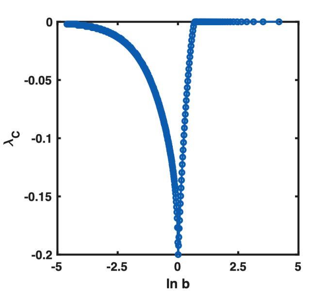
Refer to caption
Figure 8: λC​(b)\lambda_{C}(b) as a function of ln⁡b\ln b, where the hopping tt is taken as 11.

Next we define λD\lambda_{D} and λC\lambda_{C} as

λD​(b)\displaystyle\lambda_{D}(b) =\displaystyle= λ11​(b)−λ21​(b)−λ31​(b)+λ41​(b),\displaystyle\lambda_{11}(b)-\lambda_{21}(b)-\lambda_{31}(b)+\lambda_{41}(b),
λC​(b)\displaystyle\lambda_{C}(b) =\displaystyle= λ11​(b)+λ21​(b)−λ31​(b)−λ41​(b).\displaystyle\lambda_{11}(b)+\lambda_{21}(b)-\lambda_{31}(b)-\lambda_{41}(b). (77)

Using λ41=λ45\lambda_{41}=\lambda_{45}, as well as the inversion and translation symmetries, we obtain λ21=λ41\lambda_{21}=\lambda_{41}, which demonstrates that up to one-loop level there is the relation

λD​(b)=λC​(b).\displaystyle\lambda_{D}(b)=\lambda_{C}(b). (78)

Hence it enough to consider λC​(b)\lambda_{C}(b). Fig. 8 shows λC​(b)\lambda_{C}(b) as a function of ln⁡b\ln b obtained by numerically calculating the integral in Eq. (46), and it can be seen that λC​(b)\lambda_{C}(b) is always negative. We note that the integral ∫d​ln⁡b⋅λC​(b)\int d\ln b\cdot\lambda_{C}(b) converges when bb is integrated from 00 to bs∼4b_{s}\sim 4. When b≪1b\ll 1, the integration in Eq. (46) is restricted within a narrow range θ∼b\theta\sim b due to the factor f⁡(ν,m,θ,b)f(\nu,m,\theta,b). Let x=ln⁡bx=\ln b, and split ∫−∞xsd​x​λC​(x)\int_{-\infty}^{x_{s}}dx\lambda_{C}(x) as ∫−∞yd​x​λC​(x)+∫yxsd​x​λC​(x)\int_{-\infty}^{y}dx\lambda_{C}(x)+\int_{y}^{x_{s}}dx\lambda_{C}(x) where xs∼ln⁡4x_{s}\sim\ln 4 and y≪1y\ll 1. Since ∫−∞yd​x​λC​(x)\int_{-\infty}^{y}dx\lambda_{C}(x) goes like ∫−∞yd​x​ex\int_{-\infty}^{y}dxe^{x} which converges, we see that ∫−∞xsd​x​λC​(x)\int_{-\infty}^{x_{s}}dx\lambda_{C}(x) is a converging integral. As a result, we conclude from Eq. (71) and Eq. (72) that RG predicts

cC<0,hC<0,cD<0,hD<0.\displaystyle c_{C}<0,\penalty\ h_{C}<0,\penalty\ c_{D}<0,\penalty\ h_{D}<0. (79)

V.4 Comparison with numerics

Next we check if the predictions in Eq. (79) are consistent with the numerical results. The method for numerically determining the signs of the bosonization coefficients has been discussed in detail in Supplementary Materials in Ref. Yang2022b. In this subsection, we follow the method in Ref. Yang2022b. We will focus on the “C” coefficients, since they correspond to NαN^{\alpha} (α=x,y,z\alpha=x,y,z) which are relevant operators and open a spin gap at low energies. Appendix G discusses the numerical determinations of the “D” coefficients, which are not successful, and the reasons remain not clear.

Throughout this subsection, we work in the four-sublattice rotated frame and take the parameters as K+2​J=1K+2J=1, J=−1J=-1, Γ=0.35\Gamma=0.35 in accordance with Ref. Yang2022b. DMRG numerical simulations are performed on a system of L=144L=144 sites with periodic boundary conditions. The bond dimension mm and truncation error ϵ\epsilon in DMRG simulations are taken as m=1400m=1400 and ϵ=10−9\epsilon=10^{-9}.

Applying a small staggered magnetic field hπzh_{\pi}^{z} along zz-direction, the low energy Hamiltonian can be derived as −hπziC∫dxNz-h_{\pi}^{z}i_{C}\int dxN^{z}. Since NzN^{z} is a relevant operator, a spin gap opens and a nonzero expectation value ⟨Nz⟩\langle N^{z}\rangle is developed in the low energy theory. Using the nonsymmorphic bosonization formulas, the spin expectation values are

⟨S→1+4​n⟩\displaystyle\langle\vec{S}_{1+4n}\rangle =\displaystyle= ⟨Nz⟩​(−hC,hC,−iC),\displaystyle\langle N^{z}\rangle(-h_{C},h_{C},-i_{C}),
⟨S→2+4​n⟩\displaystyle\langle\vec{S}_{2+4n}\rangle =\displaystyle= ⟨Nz⟩​(−hC,−hC,iC),\displaystyle\langle N^{z}\rangle(-h_{C},-h_{C},i_{C}),
⟨S→3+4​n⟩\displaystyle\langle\vec{S}_{3+4n}\rangle =\displaystyle= ⟨Nz⟩​(hC,−hC,−iC),\displaystyle\langle N^{z}\rangle(h_{C},-h_{C},-i_{C}),
⟨S→4+4​n⟩\displaystyle\langle\vec{S}_{4+4n}\rangle =\displaystyle= ⟨Nz⟩​(hC,hC,iC).\displaystyle\langle N^{z}\rangle(h_{C},h_{C},i_{C}). (80)

Taking hπz=10−3h_{\pi}^{z}=10^{-3}, DMRG simulations are able to verify the pattern in Eq. (80), with

⟨Nz⟩​hC\displaystyle\langle N^{z}\rangle h_{C} =\displaystyle= −4.5×10⁻⁴,\displaystyle-4.5\times 10^{-4},
⟨Nz⟩​iC\displaystyle\langle N^{z}\rangle i_{C} =\displaystyle= 0.0119.\displaystyle 0.0119. (81)

This shows that

hC/iC=−0.0378.\displaystyle h_{C}/i_{C}=-0.0378. (82)

Notice that iCi_{C} is the dominant coefficient, and we expect that it does not change sign compared with the U(1) symmetric case for the microscopic Hamiltonian (i.e., when K+2​J=0K+2J=0 and Γ=0\Gamma=0). Therefore, hC<0h_{C}<0 as determined from Eq. (82), which is consistent with the prediction in Eq. (79). In addition, Table 1 gives a ratio |hC/iC||h_{C}/i_{C}| equal to 0.03800.0380 where the values are obtained from studying spin correlation functions Yang2022b. It can be seen that the two approaches (magnetic field response vs. correlation functions) are fully consistent with each other.

Next applying a small staggered magnetic field hπxh_{\pi}^{x} along xx-direction, the low energy Hamiltonian can be derived as −hπx​(aC​∫d​x​Nx−bD​∫d​x​Jy)-h_{\pi}^{x}(a_{C}\int dxN^{x}-b_{D}\int dxJ^{y}). Since the scaling dimension of NxN^{x} is smaller than that of JyJ^{y}, we expect that a nonzero expectation value ⟨Nx⟩\langle N^{x}\rangle develops in the low energy theory. Then the spin expectation values can be determined as follows from the nonsymmorphic bosonization formulas,

⟨S→1+4​n⟩\displaystyle\langle\vec{S}_{1+4n}\rangle =\displaystyle= ⟨Nx⟩​(−aC,−bC,−cC),\displaystyle\langle N^{x}\rangle(-a_{C},-b_{C},-c_{C}),
⟨S→2+4​n⟩\displaystyle\langle\vec{S}_{2+4n}\rangle =\displaystyle= ⟨Nx⟩​(aC,−bC,−cC),\displaystyle\langle N^{x}\rangle(a_{C},-b_{C},-c_{C}),
⟨S→3+4​n⟩\displaystyle\langle\vec{S}_{3+4n}\rangle =\displaystyle= ⟨Nx⟩​(−aC,−bC,cC),\displaystyle\langle N^{x}\rangle(-a_{C},-b_{C},c_{C}),
⟨S→4+4​n⟩\displaystyle\langle\vec{S}_{4+4n}\rangle =\displaystyle= ⟨Nx⟩​(aC,−bC,cC).\displaystyle\langle N^{x}\rangle(a_{C},-b_{C},c_{C}). (83)

Since aCa_{C} is the dominant coefficient, again aCa_{C} is expected to be positive. The patterns in Eq. (83) are verified by DMRG numerics, with the following values

⟨Nx⟩​aC\displaystyle\langle N^{x}\rangle a_{C} =\displaystyle= 0.0890,\displaystyle 0.0890,
⟨Nx⟩​bC\displaystyle\langle N^{x}\rangle b_{C} =\displaystyle= 1.54×10⁻⁴,\displaystyle 1.54\times 10^{-4},
⟨Nx⟩​cC\displaystyle\langle N^{x}\rangle c_{C} =\displaystyle= −0.00431,\displaystyle-0.00431, (84)

which give the ratios as

bC/aC\displaystyle b_{C}/a_{C} =\displaystyle= 0.0017,\displaystyle 0.0017,
cC/aC\displaystyle c_{C}/a_{C} =\displaystyle= −0.0484.\displaystyle-0.0484. (85)

Hence the sign of cCc_{C} is consistent with the prediction in Eq. (79). However, Table 1 gives a ratio |cC/aC|=0.189|c_{C}/a_{C}|=0.189, not consistent with the result in Eq. (85). The reason for such discrepancy is unclear, and one possibility may be the neglection of the JyJ^{y} term in the analysis.

VI Summary

In summary, we have performed an RG study on the origin of the U(1) breaking terms in the bosonization formulas in the Luttinger liquid phase of the one-dimensional spin-1/2 Kitaev-Heisenberg-Gamma model with an antiferromagnetic Kitaev interaction. The RG analysis provides explanations for the origin of the ten non-universal bosonization coefficients in the abelian bosonization formulas of the spin operators. It can also give predictions on the signs and order of magnitudes of these bosonization coefficients. Our work is helpful to understand the rich physics related to nonsymmorphic symmetries in the gapless Luttinger liquid phases of the one-dimensional Kitaev spin models.

Acknowledgements.
W.Y. and I.A. acknowledge support from NSERC Discovery Grant 04033-2016. C.X. is partially supported by Strategic Priority Research Program of CAS (No. XDB28000000). A.N. acknowledges support from the Max Planck-UBC-UTokyo Center for Quantum Materials and the Canada First Research Excellence Fund (CFREF) Quantum Materials and Future Technologies Program of the Stewart Blusson Quantum Matter Institute (SBQMI).

Appendix A Explicit forms of the Hamiltonians

The Hamiltonian in the unrotated frame is two-site periodic, which has the form

H2​n+1,2​n+2\displaystyle H_{2n+1,2n+2} =\displaystyle= K​S2​n+1x​S2​n+2x+Γ⁡(S2​n+1y​S2​n+2z+S2​n+1z​S2​n+2y)+J​S→2​n+1⋅S→2​n+2,\displaystyle KS_{2n+1}^{x}S_{2n+2}^{x}+\Gamma(S_{2n+1}^{y}S_{2n+2}^{z}+S_{2n+1}^{z}S_{2n+2}^{y})+J\vec{S}_{2n+1}\cdot\vec{S}_{2n+2},
H2​n+2,2​n+3\displaystyle H_{2n+2,2n+3} =\displaystyle= K​S2​n+2y​S2​n+3y+Γ⁡(S2​n+2z​S2​n+3x+S2​n+2x​S2​n+3z)+J​S→2​n+2⋅S→2​n+3.\displaystyle KS_{2n+2}^{y}S_{2n+3}^{y}+\Gamma(S_{2n+2}^{z}S_{2n+3}^{x}+S_{2n+2}^{x}S_{2n+3}^{z})+J\vec{S}_{2n+2}\cdot\vec{S}_{2n+3}. (86)

After the four-sublattice rotation, the Hamiltonian becomes four-site periodic, given by

H4​n+1,4​n+2′\displaystyle H^{\prime}_{4n+1,4n+2} =\displaystyle= (K+2​J)​S4​n+1x​S4​n+2x−J​S→4​n+1⋅S→4​n+2+Γ⁡(S4​n+1y​S4​n+2z+S4​n+1z​S4​n+2y),\displaystyle(K+2J)S_{4n+1}^{x}S_{4n+2}^{x}-J\vec{S}_{4n+1}\cdot\vec{S}_{4n+2}+\Gamma(S^{y}_{4n+1}S^{z}_{4n+2}+S^{z}_{4n+1}S^{y}_{4n+2}),
H4​n+2,4​n+3′\displaystyle H^{\prime}_{4n+2,4n+3} =\displaystyle= (K+2​J)​S4​n+2y​S4​n+3y−J​S→4​n+2⋅S→4​n+3+Γ⁡(S4​n+2z​S4​n+3x+S4​n+2x​S4​n+3z),\displaystyle(K+2J)S_{4n+2}^{y}S_{4n+3}^{y}-J\vec{S}_{4n+2}\cdot\vec{S}_{4n+3}+\Gamma(S^{z}_{4n+2}S^{x}_{4n+3}+S^{x}_{4n+2}S^{z}_{4n+3}),
H4​n+3,4​n+4′\displaystyle H^{\prime}_{4n+3,4n+4} =\displaystyle= (K+2​J)​S4​n+3x​S4​n+4x−J​S→4​n+3⋅S→4​n+4−Γ⁡(S4​n+3y​S4​n+4z+S4​n+3z​S4​n+4y),\displaystyle(K+2J)S_{4n+3}^{x}S_{4n+4}^{x}-J\vec{S}_{4n+3}\cdot\vec{S}_{4n+4}-\Gamma(S^{y}_{4n+3}S^{z}_{4n+4}+S^{z}_{4n+3}S^{y}_{4n+4}),
H4​n+4,4​n+5′\displaystyle H^{\prime}_{4n+4,4n+5} =\displaystyle= (K+2​J)​S4​n+4y​S4​n+5y−J​S→4​n+4⋅S→4​n+5−Γ⁡(S4​n+4z​S4​n+5x+S4​n+4x​S4​n+5z).\displaystyle(K+2J)S_{4n+4}^{y}S_{4n+5}^{y}-J\vec{S}_{4n+4}\cdot\vec{S}_{4n+5}-\Gamma(S^{z}_{4n+4}S^{x}_{4n+5}+S^{x}_{4n+4}S^{z}_{4n+5}). (87)

Appendix B Explicit forms of the nonsymmorphic bosonization formulas

In the four-sublattice rotated frame, the explicit forms of the abelian bosonization formulas in the Luttinger liquid phase in Fig. 2 are given by

S1+4​nx\displaystyle S_{1+4n}^{x} =\displaystyle= aD​Jx+bD​Jy+hD​Jz−aC​Nx−bC​Ny−hC​Nz,\displaystyle a_{D}J^{x}+b_{D}J^{y}+h_{D}J^{z}-a_{C}N^{x}-b_{C}N^{y}-h_{C}N^{z},
S1+4​ny\displaystyle S_{1+4n}^{y} =\displaystyle= bD​Jx+aD​Jy−hD​Jz−bC​Nx−aC​Ny+hC​Nz,\displaystyle b_{D}J^{x}+a_{D}J^{y}-h_{D}J^{z}-b_{C}N^{x}-a_{C}N^{y}+h_{C}N^{z},
S1+4​nz\displaystyle S_{1+4n}^{z} =\displaystyle= cD​Jx−cD​Jy+iD​Jz−cC​Nx+cC​Ny−iC​Nz,\displaystyle c_{D}J^{x}-c_{D}J^{y}+i_{D}J^{z}-c_{C}N^{x}+c_{C}N^{y}-i_{C}N^{z}, (88)
S2+4​nx\displaystyle S_{2+4n}^{x} =\displaystyle= aD​Jx−bD​Jy−hD​Jz+aC​Nx−bC​Ny−hC​Nz,\displaystyle a_{D}J^{x}-b_{D}J^{y}-h_{D}J^{z}+a_{C}N^{x}-b_{C}N^{y}-h_{C}N^{z},
S2+4​ny\displaystyle S_{2+4n}^{y} =\displaystyle= −bD​Jx+aD​Jy−hD​Jz−bC​Nx+aC​Ny−hC​Nz,\displaystyle-b_{D}J^{x}+a_{D}J^{y}-h_{D}J^{z}-b_{C}N^{x}+a_{C}N^{y}-h_{C}N^{z},
S2+4​nz\displaystyle S_{2+4n}^{z} =\displaystyle= −cD​Jx−cD​Jy+iD​Jz−cC​Nx−cC​Ny+iC​Nz,\displaystyle-c_{D}J^{x}-c_{D}J^{y}+i_{D}J^{z}-c_{C}N^{x}-c_{C}N^{y}+i_{C}N^{z}, (89)
S3+4​nx\displaystyle S_{3+4n}^{x} =\displaystyle= aD​Jx+bD​Jy−hD​Jz−aC​Nx−bC​Ny+hC​Nz,\displaystyle a_{D}J^{x}+b_{D}J^{y}-h_{D}J^{z}-a_{C}N^{x}-b_{C}N^{y}+h_{C}N^{z},
S3+4​ny\displaystyle S_{3+4n}^{y} =\displaystyle= bD​Jx+aD​Jy+hD​Jz−bC​Nx−aC​Ny−hC​Nz,\displaystyle b_{D}J^{x}+a_{D}J^{y}+h_{D}J^{z}-b_{C}N^{x}-a_{C}N^{y}-h_{C}N^{z},
S3+4​nz\displaystyle S_{3+4n}^{z} =\displaystyle= −cD​Jx+cD​Jy+iD​Jz+cC​Nx−cC​Ny−iC​Nz,\displaystyle-c_{D}J^{x}+c_{D}J^{y}+i_{D}J^{z}+c_{C}N^{x}-c_{C}N^{y}-i_{C}N^{z}, (90)
S4+4​nx\displaystyle S_{4+4n}^{x} =\displaystyle= aD​Jx−bD​Jy+hD​Jz+aC​Nx−bC​Ny+hC​Nz,\displaystyle a_{D}J^{x}-b_{D}J^{y}+h_{D}J^{z}+a_{C}N^{x}-b_{C}N^{y}+h_{C}N^{z},
S4+4​ny\displaystyle S_{4+4n}^{y} =\displaystyle= −bD​Jx+aD​Jy+hD​Jz−bC​Nx+aC​Ny+hC​Nz,\displaystyle-b_{D}J^{x}+a_{D}J^{y}+h_{D}J^{z}-b_{C}N^{x}+a_{C}N^{y}+h_{C}N^{z},
S4+4​nz\displaystyle S_{4+4n}^{z} =\displaystyle= cD​Jx+cD​Jy+iD​Jz+cC​Nx+cC​Ny+iC​Nz.\displaystyle c_{D}J^{x}+c_{D}J^{y}+i_{D}J^{z}+c_{C}N^{x}+c_{C}N^{y}+i_{C}N^{z}. (91)

Appendix C Nonabelian bosonization of 1D repulsive Hubbard model at half filling

Here we give a quick review of the nonabelian bosonization method (for details, see Ref. Affleck1988). The 1D spin-1/2 Dirac fermion exhibits the phenomenon of spin-charge separation and can be decomposed into an SU(2)1 spin boson gg and a U⁡(1)U(1) charge boson ϕ\phi, where the actions in real time for the SU(2) matrix gg and the real scalar ϕ\phi are given by

Sg\displaystyle S_{g} =\displaystyle= 18​π​∫d2​x​Tr​(∂μg−1​∂μg)+112​π​∫d3​x​ϵμ​ν​λ​Tr​(g~−1​∂μg~​g~−1​∂νg~​g~−1​∂λg~),\displaystyle\frac{1}{8\pi}\int d^{2}x\text{Tr}(\partial_{\mu}g^{-1}\partial^{\mu}g)+\frac{1}{12\pi}\int d^{3}x\epsilon^{\mu\nu\lambda}\text{Tr}(\tilde{g}^{-1}\partial_{\mu}\tilde{g}\tilde{g}^{-1}\partial_{\nu}\tilde{g}\tilde{g}^{-1}\partial_{\lambda}\tilde{g}),
Sϕ\displaystyle S_{\phi} =\displaystyle= 12​∫d2​x​∂μϕ​∂μϕ,\displaystyle\frac{1}{2}\int d^{2}x\partial_{\mu}\phi\partial^{\mu}\phi, (92)

in which g~\tilde{g} is an extension of gg from two-dimensional spacetime to three-dimension, and the velocities in SgS_{g} and SϕS_{\phi} have been absorbed into a redefinition of time. We note that because of the topological nature of the second term (i.e., WZW term) in SgS_{g}, the partition function does not depend on the way of extension. In terms of gg and ϕ\phi, the hopping term between the left and right movers can be bosonized as follows

cL​cR†=const.​g​ei​2​π​ϕ,\displaystyle c_{L}c_{R}^{\dagger}=\text{const.}ge^{i\sqrt{2\pi}\phi}, (93)

where const. is a real constant. When a repulsive Hubbard interaction U>0U>0 is introduced, SgS_{g} and SϕS_{\phi} are changed into

Sg′=Sg+2​Ut​∫d2​x​J→L⋅J→R,\displaystyle S_{g}^{\prime}=S_{g}+\frac{2U}{t}\int d^{2}x\vec{J}_{L}\cdot\vec{J}_{R},
Sϕ′=12​(1+U2​π​t)​∫d2​x​∂μϕ​∂μϕ−λϕ​U​∫d2​x​cos⁡(8​π​ϕ),\displaystyle S_{\phi}^{\prime}=\frac{1}{2}(1+\frac{U}{2\pi t})\int d^{2}x\partial_{\mu}\phi\partial^{\mu}\phi-\lambda_{\phi}U\int d^{2}x\cos(\sqrt{8\pi}\phi), (94)

in which λϕ>0\lambda_{\phi}>0 is a constant, and the WZW current operators J→L\vec{J}_{L} and J→R\vec{J}_{R} are defined as

J→L\displaystyle\vec{J}_{L} =\displaystyle= i4​π​Tr​(∂+g⋅g−1​σ→),\displaystyle\frac{i}{4\pi}\text{Tr}(\partial_{+}g\cdot g^{-1}\vec{\sigma}),
J→R\displaystyle\vec{J}_{R} =\displaystyle= −i4​π​Tr​(g−1​∂−g​σ→),\displaystyle-\frac{i}{4\pi}\text{Tr}(g^{-1}\partial_{-}g\vec{\sigma}), (95)

where ∂±=∂t±∂x\partial_{\pm}=\partial_{t}\pm\partial_{x}. It can be shown that the spin sector remains gapless since J→L⋅J→R\vec{J}_{L}\cdot\vec{J}_{R} is marginally irrelevant. However, a gap opens in the charge sector since the cos⁡(8​π​ϕ)\cos(\sqrt{8\pi}\phi) term is relevant at low energies. The scaling of the charge gap can be solved as mc∼e−U/(πt)m_{c}\sim e^{-U/(\pi t)}.

The above analysis shows that in the weak-UU limit, the low energy physics of the 1D repulsive Hubbard model is described by the SU(2)1 WZW theory. On the other hand, we know that according to the standard second order perturbation, the large-UU limit reduces to the SU(2) AFM Heisenberg model. Since there is no phase transition between the weak-UU and large-UU limits, the low energy physics of the SU(2) AFM Heisenberg model is also described by the SU(2)1 WZW theory. This provides a nonabelian bosonization description for the low energy physics of the AFM Heisenberg model in 1D.

Appendix D Evaluation of Feynman diagrams

D.1 Evaluation of diagram in Fig. 5

We need to express the interactions and the spin operators in the frequency and momentum space. The interaction term is

∫d​τ​∑nSi+4​nα​(τ)​Sj+4​nβ​(τ)=\displaystyle\int d\tau\sum_{n}S_{i+4n}^{\alpha}(\tau)S_{j+4n}^{\beta}(\tau)=
1N​β​∫d​τ​∑n∑k1,k2,k3,k4c†​(k1)​12​σα​c​(k2)⋅c†​(k3)​12​σβ​c​(k4)​ei⁡(ω1−ω2+ω3−ω4)​τ​ei⁡(k→1−k→2)⋅(i+4​n)​a​x^​ei⁡(k→3−k→4)⋅(j+4​n)​a​x^,\displaystyle\frac{1}{N\beta}\int d\tau\sum_{n}\sum_{k_{1},k_{2},k_{3},k_{4}}c^{\dagger}(k_{1})\frac{1}{2}\sigma^{\alpha}c(k_{2})\cdot c^{\dagger}(k_{3})\frac{1}{2}\sigma^{\beta}c(k_{4})e^{i(\omega_{1}-\omega_{2}+\omega_{3}-\omega_{4})\tau}e^{i(\vec{k}_{1}-\vec{k}_{2})\cdot(i+4n)a\hat{x}}e^{i(\vec{k}_{3}-\vec{k}_{4})\cdot(j+4n)a\hat{x}}, (96)

in which k=(i​ω,k→)k=(i\omega,\vec{k}) where ω\omega is Matsubara frequency and k→\vec{k} is the wavevector in space (we define the spatial wavevector as a vector to distinguish it from the spacetime combined index kk, even though the system is 1D and k→\vec{k} is in essence a scalar), aa is the lattice spacing, NN is the system size, β\beta is the inverse of the temperature, nn is summed over the unit cells, and x^\hat{x} is the unit vector in the spatial direction. Using the identity

1N​∑nei⁡(k→1−k→2+k→3−k→4)⋅4​n​a​x^=14​∑m=14δk→1−k→2+k→3−k→4,π2​a​m​x^,\displaystyle\frac{1}{N}\sum_{n}e^{i(\vec{k}_{1}-\vec{k}_{2}+\vec{k}_{3}-\vec{k}_{4})\cdot 4na\hat{x}}=\frac{1}{4}\sum_{m=1}^{4}\delta_{\vec{k}_{1}-\vec{k}_{2}+\vec{k}_{3}-\vec{k}_{4},\frac{\pi}{2a}m\hat{x}}, (97)

Eq. (96) can be written as

ΔN​β​14​∑m∑k1,k2,k3,k4ei⁡(k→1−k→2)⋅(i−j)​a​x^​e−i​π2​m​j​δk1−k2+k3−k4+π2​a​m​x^,0​c†​(k1)​12​σα​c​(k2)⋅c†​(k3)​12​σβ​c​(k4),\displaystyle\frac{\Delta}{N\beta}\frac{1}{4}\sum_{m}\sum_{k_{1},k_{2},k_{3},k_{4}}e^{i(\vec{k}_{1}-\vec{k}_{2})\cdot(i-j)a\hat{x}}e^{-i\frac{\pi}{2}mj}\delta_{k_{1}-k_{2}+k_{3}-k_{4}+\frac{\pi}{2a}m\hat{x},0}c^{\dagger}(k_{1})\frac{1}{2}\sigma^{\alpha}c(k_{2})\cdot c^{\dagger}(k_{3})\frac{1}{2}\sigma^{\beta}c(k_{4}), (98)

i.e.,

ΔN​β​14​∑m∑k​k′​qei​q→⋅(i−j)​a​x^​e−i​π2​m​j​c†​(k+q)​12​σα​c​(k)⋅c†​(k′−q)​12​σβ​c​(k′+π2​a​m​x^),\displaystyle\frac{\Delta}{N\beta}\frac{1}{4}\sum_{m}\sum_{kk^{\prime}q}e^{i\vec{q}\cdot(i-j)a\hat{x}}e^{-i\frac{\pi}{2}mj}c^{\dagger}(k+q)\frac{1}{2}\sigma^{\alpha}c(k)\cdot c^{\dagger}(k^{\prime}-q)\frac{1}{2}\sigma^{\beta}c(k^{\prime}+\frac{\pi}{2a}m\hat{x}), (99)

where

c†​(k)=1N​β​∫d​τ​∑j=1Ncj†​(τ)​ei⁡(ω​τ−k→⋅j​a​x^).\displaystyle c^{\dagger}(k)=\frac{1}{\sqrt{N\beta}}\int d\tau\sum_{j=1}^{N}c^{\dagger}_{j}(\tau)e^{i(\omega\tau-\vec{k}\cdot ja\hat{x})}. (100)

By defining the Fourier transform hlα​(q)h_{l}^{\alpha}(q) as

hlα​(q)=1N​β​∫d​τ​∑n=1N/4hlα​(τ,n)​ei⁡(ω​τ−q→⋅4​n​a​x^),\displaystyle h_{l}^{\alpha}(q)=\frac{1}{\sqrt{N\beta}}\int d\tau\sum_{n=1}^{N/4}h_{l}^{\alpha}(\tau,n)e^{i(\omega\tau-\vec{q}\cdot 4na\hat{x})}, (101)

the coupling to the magnetic field becomes

∫d​τ​∑nhlα​(τ,n)​Sl+4​nα​(τ)=14​∑k​q∑mei​q→⋅l​a​x^​ei​π2​m​l​hlα​(−q)​c†​(k+π2​a​m​x^)​12​σα​c​(k−q).\displaystyle\int d\tau\sum_{n}h_{l}^{\alpha}(\tau,n)S_{l+4n}^{\alpha}(\tau)=\frac{1}{4}\sum_{kq}\sum_{m}e^{i\vec{q}\cdot la\hat{x}}e^{i\frac{\pi}{2}ml}h_{l}^{\alpha}(-q)c^{\dagger}(k+\frac{\pi}{2a}m\hat{x})\frac{1}{2}\sigma^{\alpha}c(k-q). (102)

Notice that q→∈[0,π2​a)\vec{q}\in[0,\frac{\pi}{2a}) in hlα​(q)h_{l}^{\alpha}(q) since hlα​(n)h_{l}^{\alpha}(n) is defined every four sites.

We set the momentum transfer q→′\vec{q}^{\prime} in hlα​(q′)h_{l}^{\alpha}(q^{\prime}) as |q→′|∼0|\vec{q}^{\prime}|\sim 0 (both SuαS_{u}^{\alpha} and SsαS_{s}^{\alpha} correspond to |q→′|∼0|\vec{q}^{\prime}|\sim 0, which is the reason why they are not separated above the energy scale Λs\Lambda_{s}). The expression corresponding to the diagram in Fig. 5 is given by

14​N​β∑me−i​π2​m​j∑k​p​qei​q→⋅(i−j)​a​x^c†(k+q)12σμc(k)⋅14∑k′​q′​m′ei​q→′⋅l​a​x^ei​π2​m′​lhlα(−q′)\displaystyle\frac{1}{4N\beta}\sum_{m}e^{-i\frac{\pi}{2}mj}\sum_{kpq}e^{i\vec{q}\cdot(i-j)a\hat{x}}c^{\dagger}(k+q)\frac{1}{2}\sigma^{\mu}c(k)\cdot\frac{1}{4}\sum_{k^{\prime}q^{\prime}m^{\prime}}e^{i\vec{q}^{\prime}\cdot la\hat{x}}e^{i\frac{\pi}{2}m^{\prime}l}h_{l}^{\alpha}(-q^{\prime})
×⟨c†​(p−q)​12​σν​c​(p+π2​a​m​x^)​c†​(k′+π2​a​m′​x^)​12​σα​c​(k′−q′)⟩f.\displaystyle\times\langle c^{\dagger}(p-q)\frac{1}{2}\sigma^{\nu}c(p+\frac{\pi}{2a}m\hat{x})c^{\dagger}(k^{\prime}+\frac{\pi}{2a}m^{\prime}\hat{x})\frac{1}{2}\sigma^{\alpha}c(k^{\prime}-q^{\prime})\rangle_{\text{f}}. (103)

Since the free fermion propagator is diagonal in the frequency-momentum space, there are the following constraints (m¯=1,2,3,4\bar{m}=1,2,3,4)

m′=m+m¯,p=k′+π2​a​m¯,q=q′+π2​a​m¯.\displaystyle m^{\prime}=m+\bar{m},\penalty\ p=k^{\prime}+\frac{\pi}{2a}\bar{m},\penalty\ q=q^{\prime}+\frac{\pi}{2a}\bar{m}. (104)

Plugging Eq. (104) into Eq. (103) and rearranging the terms, we obtain the following alternative expression for Eq. (103),

14∑m¯ei​π2​m¯​i∑k​q′ei​q→′⋅i​a​x^hlα(−q′)c†(k+q′+π2​am¯x^)12σμc(k)e−iq→′⋅(j−l)ax^\displaystyle\frac{1}{4}\sum_{\bar{m}}e^{i\frac{\pi}{2}\bar{m}i}\sum_{kq^{\prime}}e^{i\vec{q}^{\prime}\cdot ia\hat{x}}h_{l}^{\alpha}(-q^{\prime})c^{\dagger}(k+q^{\prime}+\frac{\pi}{2a}\bar{m}\hat{x})\frac{1}{2}\sigma^{\mu}c(k)e^{-i\vec{q}^{\prime}\cdot(j-l)a\hat{x}}
×14​N​β​∑m∑k′e−i​π2​(m+m¯)​(j−l)​⟨c†​(k′−q′)​12​σν​c​(k′+π2​a​(m+m¯)​x^)​c†​(k′+π2​a​(m+m¯)​x^)​12​σα​c​(k′−q′)⟩f.\displaystyle\times\frac{1}{4N\beta}\sum_{m}\sum_{k^{\prime}}e^{-i\frac{\pi}{2}(m+\bar{m})(j-l)}\langle c^{\dagger}(k^{\prime}-q^{\prime})\frac{1}{2}\sigma^{\nu}c(k^{\prime}+\frac{\pi}{2a}(m+\bar{m})\hat{x})c^{\dagger}(k^{\prime}+\frac{\pi}{2a}(m+\bar{m})\hat{x})\frac{1}{2}\sigma^{\alpha}c(k^{\prime}-q^{\prime})\rangle_{\text{f}}. (105)

In Eq. (105), the factor e−iq→′⋅(j−l)ax^e^{-i\vec{q}^{\prime}\cdot(j-l)a\hat{x}} can be set as 11 since q→′\vec{q}^{\prime} is a slowly varying variable. In fact, if we expand the exponential e−iq→′⋅(j−l)ax^e^{-i\vec{q}^{\prime}\cdot(j-l)a\hat{x}}, |q→′|n|\vec{q}^{\prime}|^{n} becomes gradients in the real space, which renders the n≠0n\neq 0 terms less relevant than the leading n=0n=0 term in the RG sense. This justifies in a more rigorous way why e−iq→′⋅(j−l)ax^e^{-i\vec{q}^{\prime}\cdot(j-l)a\hat{x}} can be taken as 11.

Then by using Eq. (102), it can be checked that Eq. (105) becomes

λj​l​δν​α​Δ​ln⁡b⋅∫d​τ​∑nhlμ​(τ,n)​Su,lμ​(τ,n),\displaystyle\lambda_{jl}\delta_{\nu\alpha}\Delta\ln b\cdot\int d\tau\sum_{n}h_{l}^{\mu}(\tau,n)S_{u,l}^{\mu}(\tau,n), (106)

in which

λj​lΔlnb=−a8∑me−i​π2​m​(j−l)∫Λ/b′Λ/bd2k𝒢(k)𝒢(k+π2​amx^),\displaystyle\lambda_{jl}\Delta\ln b=-\frac{a}{8}\sum_{m}e^{-i\frac{\pi}{2}m(j-l)}\int_{\Lambda/b^{\prime}}^{\Lambda/b}d^{2}k\mathcal{G}(k)\mathcal{G}(k+\frac{\pi}{2a}m\hat{x}), (107)

where 𝒢⁡(k)\mathcal{G}(k) is the free fermion Green’s function defined as

𝒢⁡(k)=1i​ω−ϵ⁡(k).\displaystyle\mathcal{G}(k)=\frac{1}{i\omega-\epsilon(k)}. (108)

In Eq. (108), ϵ⁡(k)\epsilon(k) is the free fermion dispersion which includes the chemical potential term.

D.2 Evaluation of diagram in Fig. 6

The expression corresponding to Fig. 6 is

116​N​β​∑k​p​q∑m∑k′​q′∑m′e−i​π2​m​j​ei​π2​m′​l​ei​q→⋅(i−j)​a​x^​ei​q→′⋅l​a​x^​hlα​(−q′)\displaystyle\frac{1}{16N\beta}\sum_{kpq}\sum_{m}\sum_{k^{\prime}q^{\prime}}\sum_{m^{\prime}}e^{-i\frac{\pi}{2}mj}e^{i\frac{\pi}{2}m^{\prime}l}e^{i\vec{q}\cdot(i-j)a\hat{x}}e^{i\vec{q}^{\prime}\cdot la\hat{x}}h_{l}^{\alpha}(-q^{\prime})
×c†​(k+q)​12​σμ​⟨c⁡(k)​c†​(k′+π2​a​m′)​12​σα​c​(k′−q′)​c†​(p−q−π2​a​m)⟩f​12​σν​c​(p).\displaystyle\times c^{\dagger}(k+q)\frac{1}{2}\sigma^{\mu}\langle c(k)c^{\dagger}(k^{\prime}+\frac{\pi}{2a}m^{\prime})\frac{1}{2}\sigma^{\alpha}c(k^{\prime}-q^{\prime})c^{\dagger}(p-q-\frac{\pi}{2a}m)\rangle_{f}\frac{1}{2}\sigma^{\nu}c(p). (109)

Momentum conservation requires

k\displaystyle k =\displaystyle= k′+π2​a​(m+m¯),\displaystyle k^{\prime}+\frac{\pi}{2a}(m+\bar{m}),
q\displaystyle q =\displaystyle= p−k′+q′−π2​a​m,\displaystyle p-k^{\prime}+q^{\prime}-\frac{\pi}{2a}m,
m′\displaystyle m^{\prime} =\displaystyle= m+m¯.\displaystyle m+\bar{m}. (110)

Then it can be shown that Eq. (109) becomes

116​N​β​∑p​q′∑m¯ei​π2​m¯​i​ei​p→⋅(i−j)​a​x^​ei​q→′⋅(i−j+l)​a​x^​hlα​(−q′)​c†​(p+q′+π2​a​m¯)​12​σμ​σα​σν​c​(p)\displaystyle\frac{1}{16N\beta}\sum_{pq^{\prime}}\sum_{\bar{m}}e^{i\frac{\pi}{2}\bar{m}i}e^{i\vec{p}\cdot(i-j)a\hat{x}}e^{i\vec{q}^{\prime}\cdot(i-j+l)a\hat{x}}h_{l}^{\alpha}(-q^{\prime})c^{\dagger}(p+q^{\prime}+\frac{\pi}{2a}\bar{m})\frac{1}{2}\sigma^{\mu}\sigma^{\alpha}\sigma^{\nu}c(p)
×14∑k′∑me−ik→′⋅(i−j)ax^ei​π2​(m+m¯)​(l−i)2𝒢(k′+π2​a(m+m¯)x^)𝒢(k′−q′),\displaystyle\times\frac{1}{4}\sum_{k^{\prime}}\sum_{m}e^{-i\vec{k}^{\prime}\cdot(i-j)a\hat{x}}e^{i\frac{\pi}{2}(m+\bar{m})(l-i)}2\mathcal{G}(k^{\prime}+\frac{\pi}{2a}(m+\bar{m})\hat{x})\mathcal{G}(k^{\prime}-q^{\prime}), (111)

in which the factor of two before the Green’s function comes from the sum over the spin degree of freedom, and ∑k′\sum_{k^{\prime}} is restricted within the momentum shell, i.e., the fast modes. Notice that

∫d​τ​∑nci+4​n†​12​σρ​cj+4​n​hi​jρ​(n)=14​N​β​∑p​q′∑m¯ei​p→⋅(i−j)​a​x^​ei​q→′⋅i​a​x^​ei​π2​m¯​i​hi​j​(−q′)​c†​(p+q′+π2​a​m¯)​12​σρ​c​(p).\displaystyle\int d\tau\sum_{n}c^{\dagger}_{i+4n}\frac{1}{2}\sigma^{\rho}c_{j+4n}h_{ij}^{\rho}(n)=\frac{1}{4N\beta}\sum_{pq^{\prime}}\sum_{\bar{m}}e^{i\vec{p}\cdot(i-j)a\hat{x}}e^{i\vec{q}^{\prime}\cdot ia\hat{x}}e^{i\frac{\pi}{2}\bar{m}i}h_{ij}(-q^{\prime})c^{\dagger}(p+q^{\prime}+\frac{\pi}{2a}\bar{m})\frac{1}{2}\sigma^{\rho}c(p). (112)

Plugging Eq. (112) into Eq. (111) and neglecting the ei​q→′⋅(−j+l)​a​x^e^{i\vec{q}^{\prime}\cdot(-j+l)a\hat{x}} factor in Eq. (111) since q→′\vec{q}^{\prime} is a very small wavevector, we obtain

λi​l​j​Δ​ln⁡b​∫d​τ​∑nhi​jμ⋅α⋅ν​Sl+4​nμ⋅α⋅ν​(τ),\displaystyle\lambda_{ilj}\Delta\ln b\int d\tau\sum_{n}h_{ij}^{\mu\cdot\alpha\cdot\nu}S_{l+4n}^{\mu\cdot\alpha\cdot\nu}(\tau), (113)

where the coefficient λi​l​j\lambda_{ilj} is

λi​l​jΔlnb=a8∑mei​π2​m​(l−i)∫Λ/bΛd2k′e−ik→′⋅(i−j)ax^𝒢(k′)𝒢(k′+π2​amx^).\displaystyle\lambda_{ilj}\Delta\ln b=\frac{a}{8}\sum_{m}e^{i\frac{\pi}{2}m(l-i)}\int_{\Lambda/b}^{\Lambda}d^{2}k^{\prime}e^{-i\vec{k}^{\prime}\cdot(i-j)a\hat{x}}\mathcal{G}(k^{\prime})\mathcal{G}(k^{\prime}+\frac{\pi}{2a}m\hat{x}). (114)

Notice that shifting ll by a multiple of 44 does not affect the result in Eq. (114), hence we can impose the condition l≥min⁡{i,j}l\geq\min\{i,j\}. Apparently, Eq. (114) is invariant under spatial translation (i,j,l→i+t,j+t,l+ti,j,l\rightarrow i+t,j+t,l+t) and inversion (i,j,l→−i,−l,−ji,j,l\rightarrow-i,-l,-j), as it must be.

Appendix E Explicit RG flow equations

The explicit flow equations for hlμh_{l}^{\mu} (1≤l≤41\leq l\leq 4 and μ=x,y,z\mu=x,y,z) are

d​h1xd​ln⁡b\displaystyle\frac{dh_{1}^{x}}{d\ln b} =\displaystyle= h1x−(K+2​J)​∑jλ2​j​hjx+Γ​∑jλ4​j​hjz,\displaystyle h_{1}^{x}-(K+2J)\sum_{j}\lambda_{2j}h_{j}^{x}+\Gamma\sum_{j}\lambda_{4j}h_{j}^{z},
d​h1yd​ln⁡b\displaystyle\frac{dh_{1}^{y}}{d\ln b} =\displaystyle= h1y−(K+2​J)​∑jλ4​j​hjy−Γ​∑jλ2​j​hjz,\displaystyle h_{1}^{y}-(K+2J)\sum_{j}\lambda_{4j}h_{j}^{y}-\Gamma\sum_{j}\lambda_{2j}h_{j}^{z},
d​h1zd​ln⁡b\displaystyle\frac{dh_{1}^{z}}{d\ln b} =\displaystyle= h1z+Γ​∑jλ4​j​hjx−Γ​∑jλ2​j​hjy,\displaystyle h_{1}^{z}+\Gamma\sum_{j}\lambda_{4j}h_{j}^{x}-\Gamma\sum_{j}\lambda_{2j}h_{j}^{y}, (115)
d​h2xd​ln⁡b\displaystyle\frac{dh_{2}^{x}}{d\ln b} =\displaystyle= h2x−(K+2​J)​∑jλ1​j​hjx−Γ​∑jλ3​j​hjz,\displaystyle h_{2}^{x}-(K+2J)\sum_{j}\lambda_{1j}h_{j}^{x}-\Gamma\sum_{j}\lambda_{3j}h_{j}^{z},
d​h2yd​ln⁡b\displaystyle\frac{dh_{2}^{y}}{d\ln b} =\displaystyle= h2y−(K+2​J)​∑jλ3​j​hjy−Γ​∑jλ1​j​hjz,\displaystyle h_{2}^{y}-(K+2J)\sum_{j}\lambda_{3j}h_{j}^{y}-\Gamma\sum_{j}\lambda_{1j}h_{j}^{z},
d​h2zd​ln⁡b\displaystyle\frac{dh_{2}^{z}}{d\ln b} =\displaystyle= h2z−Γ​∑jλ3​j​hjx−Γ​∑jλ1​j​hjy,\displaystyle h_{2}^{z}-\Gamma\sum_{j}\lambda_{3j}h_{j}^{x}-\Gamma\sum_{j}\lambda_{1j}h_{j}^{y}, (116)
d​h3xd​ln⁡b\displaystyle\frac{dh_{3}^{x}}{d\ln b} =\displaystyle= h3x−(K+2​J)​∑jλ4​j​hjx−Γ​∑jλ2​j​hjz,\displaystyle h_{3}^{x}-(K+2J)\sum_{j}\lambda_{4j}h_{j}^{x}-\Gamma\sum_{j}\lambda_{2j}h_{j}^{z},
d​h3yd​ln⁡b\displaystyle\frac{dh_{3}^{y}}{d\ln b} =\displaystyle= h3y−(K+2​J)​∑jλ2​j​hjy+Γ​∑jλ4​j​hjz,\displaystyle h_{3}^{y}-(K+2J)\sum_{j}\lambda_{2j}h_{j}^{y}+\Gamma\sum_{j}\lambda_{4j}h_{j}^{z},
d​h3zd​ln⁡b\displaystyle\frac{dh_{3}^{z}}{d\ln b} =\displaystyle= h3z−Γ​∑jλ2​j​hjx+Γ​∑jλ4​j​hjy,\displaystyle h_{3}^{z}-\Gamma\sum_{j}\lambda_{2j}h_{j}^{x}+\Gamma\sum_{j}\lambda_{4j}h_{j}^{y}, (117)
d​h4xd​ln⁡b\displaystyle\frac{dh_{4}^{x}}{d\ln b} =\displaystyle= h4x−(K+2​J)​∑jλ3​j​hjx+Γ​∑jλ1​j​hjz,\displaystyle h_{4}^{x}-(K+2J)\sum_{j}\lambda_{3j}h_{j}^{x}+\Gamma\sum_{j}\lambda_{1j}h_{j}^{z},
d​h4yd​ln⁡b\displaystyle\frac{dh_{4}^{y}}{d\ln b} =\displaystyle= h4y−(K+2​J)​∑jλ1​j​hjy+Γ​∑jλ3​j​hjz,\displaystyle h_{4}^{y}-(K+2J)\sum_{j}\lambda_{1j}h_{j}^{y}+\Gamma\sum_{j}\lambda_{3j}h_{j}^{z},
d​h4zd​ln⁡b\displaystyle\frac{dh_{4}^{z}}{d\ln b} =\displaystyle= h4z+Γ​∑jλ1​j​hjx+Γ​∑jλ3​j​hjy,\displaystyle h_{4}^{z}+\Gamma\sum_{j}\lambda_{1j}h_{j}^{x}+\Gamma\sum_{j}\lambda_{3j}h_{j}^{y}, (118)

in which λ41\lambda_{41} and λ14\lambda_{14} should be understood as λ45\lambda_{45} and λ54\lambda_{54}, respectively.

Appendix F Invariance of RG flow equations under symmetries

Apparently, Eqs. (49) does not respect the U(1) symmetry. We will verify that they are invariant under the nonsymmorphic symmetries in Eq. (4).

1) Eq. (49) remains invariant under hlμ→−hlμh_{l}^{\mu}\rightarrow-h_{l}^{\mu}, hence time reversal symmetry is satisfied.

2) Suppose we shift ll to l+1l+1, and perform the rotation on spin indices by Rz=R⁡(z^,−π2)R_{z}=R(\hat{z},-\frac{\pi}{2}), then Eq. (49) becomes

d​hl+1Rz​μd​ln⁡b\displaystyle\frac{dh_{l+1}^{R_{z}\mu}}{d\ln b} =\displaystyle= hl+1Rz​μ−∑γ,k(K+2​J)​[δl+1,i​δRz​μ,γ​λj​k​hkγ+δl+1,j​δRz​μ,γ​λi​k​hkγ]\displaystyle h_{l+1}^{R_{z}\mu}-\sum_{\gamma,k}(K+2J)\big[\delta_{l+1,i}\delta_{R_{z}\mu,\gamma}\lambda_{jk}h_{k}^{\gamma}+\delta_{l+1,j}\delta_{R_{z}\mu,\gamma}\lambda_{ik}h_{k}^{\gamma}\big]
−∑γ,kϵ(γ)[δl+1,iδRz​μ,αλj​khkβ+δl+1,jδRz​μ,βλi​khkα+δl+1,iδRz​μ,βλj​khkα+δl+1,jδRz​μ,αλi​khkβ].\displaystyle-\sum_{\gamma,k}\epsilon(\gamma)\big[\delta_{l+1,i}\delta_{R_{z}\mu,\alpha}\lambda_{jk}h_{k}^{\beta}+\delta_{l+1,j}\delta_{R_{z}\mu,\beta}\lambda_{ik}h_{k}^{\alpha}+\delta_{l+1,i}\delta_{R_{z}\mu,\beta}\lambda_{jk}h_{k}^{\alpha}+\delta_{l+1,j}\delta_{R_{z}\mu,\alpha}\lambda_{ik}h_{k}^{\beta}\big].

Define Rz′R_{z}^{\prime} as Rz′​(x,y,x¯,y¯)=(y,x¯,y¯,x)R_{z}^{\prime}(x,y,\bar{x},\bar{y})=(y,\bar{x},\bar{y},x). Then <i+1,j+1>=Rz′γ\mathopen{<}i+1,j+1\mathclose{>}=R^{\prime}_{z}\gamma. Notice that Rz​α≠Rz​β≠Rz​γR_{z}\alpha\neq R_{z}\beta\neq R_{z}\gamma if α≠β≠γ\alpha\neq\beta\neq\gamma, and ϵ⁡(Rz′​γ)=(−)i−1​ϵ​(γ)\epsilon(R_{z}^{\prime}\gamma)=(-)^{i-1}\epsilon(\gamma) where γ=<i,j>\gamma=<i,j>. Then we can change the dummy variable from γ\gamma to Rz′​γR_{z}^{\prime}\gamma and also from kk to k+1k+1. As a result, Eq. () becomes

d​hl+1Rz​μd​ln⁡b\displaystyle\frac{dh_{l+1}^{R_{z}\mu}}{d\ln b} =\displaystyle= hl+1Rz​μ−∑γ,k(K+2​J)​[δl+1,i+1​δRz​μ,Rz​γ​λj+1,k+1​hk+1Rz​γ+δl+1,j+1​δRz​μ,Rz​γ​λi+1,k+1​hk+1Rz​γ]\displaystyle h_{l+1}^{R_{z}\mu}-\sum_{\gamma,k}(K+2J)\big[\delta_{l+1,i+1}\delta_{R_{z}\mu,R_{z}\gamma}\lambda_{j+1,k+1}h_{k+1}^{R_{z}\gamma}+\delta_{l+1,j+1}\delta_{R_{z}\mu,R_{z}\gamma}\lambda_{i+1,k+1}h_{k+1}^{R_{z}\gamma}\big] (120)
−(−)i−1∑γ,kϵ(γ)[δl+1,i+1δRz​μ,Rz​αλj+1,k+1hk+1Rz​β+δl+1,j+1δRz​μ,Rz​βλi+1,k+1hk+1Rz​α\displaystyle-(-)^{i-1}\sum_{\gamma,k}\epsilon(\gamma)\big[\delta_{l+1,i+1}\delta_{R_{z}\mu,R_{z}\alpha}\lambda_{j+1,k+1}h_{k+1}^{R_{z}\beta}+\delta_{l+1,j+1}\delta_{R_{z}\mu,R_{z}\beta}\lambda_{i+1,k+1}h_{k+1}^{R_{z}\alpha}
+δl+1,i+1δRz​μ,Rz​βλj+1,k+1hk+1Rz​α+δl+1,j+1δRz​μ,Rz​αλi+1,k+1hk+1Rz​β],\displaystyle+\delta_{l+1,i+1}\delta_{R_{z}\mu,R_{z}\beta}\lambda_{j+1,k+1}h_{k+1}^{R_{z}\alpha}+\delta_{l+1,j+1}\delta_{R_{z}\mu,R_{z}\alpha}\lambda_{i+1,k+1}h_{k+1}^{R_{z}\beta}\big],

in which ii, jj, α\alpha, β\beta have been changed to i+1i+1, j+1j+1, Rz​αR_{z}\alpha, Rz​βR_{z}\beta, respectively, in accordance with changing γ\gamma to Rz​γR_{z}\gamma. Using λj​k=λj+1,k+1\lambda_{jk}=\lambda_{j+1,k+1} and δμ​γ=δRz​μ,Rz​γ\delta_{\mu\gamma}=\delta_{R_{z}\mu,R_{z}\gamma}, we obtain

d​hl+1Rz​μd​ln⁡b\displaystyle\frac{dh_{l+1}^{R_{z}\mu}}{d\ln b} =\displaystyle= hl+1Rz​μ−∑γ,k(K+2​J)​[δl​i​δμ​γ​λj​k​hk+1Rz​γ+δl​j​δμ​γ​λi​k​hk+1Rz​γ]\displaystyle h_{l+1}^{R_{z}\mu}-\sum_{\gamma,k}(K+2J)\big[\delta_{li}\delta_{\mu\gamma}\lambda_{jk}h_{k+1}^{R_{z}\gamma}+\delta_{lj}\delta_{\mu\gamma}\lambda_{ik}h_{k+1}^{R_{z}\gamma}\big]
−∑γ,k(−)i−1ϵ(γ)[δl​iδμ​αλj​khk+1Rz​β+δl​jδμ​βλi​khk+1Rz​α+δl​iδμ​βλj​khk+1Rz​α+δl​jδμ​αλi​khk+1Rz​β].\displaystyle-\sum_{\gamma,k}(-)^{i-1}\epsilon(\gamma)\big[\delta_{li}\delta_{\mu\alpha}\lambda_{jk}h_{k+1}^{R_{z}\beta}+\delta_{lj}\delta_{\mu\beta}\lambda_{ik}h_{k+1}^{R_{z}\alpha}+\delta_{li}\delta_{\mu\beta}\lambda_{jk}h_{k+1}^{R_{z}\alpha}+\delta_{lj}\delta_{\mu\alpha}\lambda_{ik}h_{k+1}^{R_{z}\beta}\big].

Using the fact that the site index ii in Eq. (123) is the left point of the bond γ\gamma, we see that

(−)i−1=(−)δα,x+δβ,x.\displaystyle(-)^{i-1}=(-)^{\delta_{\alpha,x}+\delta_{\beta,x}}. (122)

Hence, we note that the sign factor (−)i−1(-)^{i-1} in the second term in the right hand side of Eq. (123) can be replaced by either (−)δμ,x+δβ,x(-)^{\delta_{\mu,x}+\delta_{\beta,x}} (for the hk+1Rz​βh_{k+1}^{R_{z}\beta} term), or (−)δμ,x+δα,x(-)^{\delta_{\mu,x}+\delta_{\alpha,x}} (for the hk+1Rz​αh_{k+1}^{R_{z}\alpha} term), since in whichever case the sign factor is (−)δα,x+δβ,x(-)^{\delta_{\alpha,x}+\delta_{\beta,x}} because of the Kronecker delta δμ​α\delta_{\mu\alpha} (for the hk+1Rz​βh_{k+1}^{R_{z}\beta} term), and δμ​β\delta_{\mu\beta} (for the hk+1Rz​αh_{k+1}^{R_{z}\alpha} term). Therefore, Eq. (123) can be re-written as

d​hl+1Rz​μd​ln⁡b\displaystyle\frac{dh_{l+1}^{R_{z}\mu}}{d\ln b} =\displaystyle= hl+1Rz​μ−∑γ,k(K+2​J)​[δl​i​δμ​γ​λj​k​hk+1Rz​γ+δl​j​δμ​γ​λi​k​hk+1Rz​γ]\displaystyle h_{l+1}^{R_{z}\mu}-\sum_{\gamma,k}(K+2J)\big[\delta_{li}\delta_{\mu\gamma}\lambda_{jk}h_{k+1}^{R_{z}\gamma}+\delta_{lj}\delta_{\mu\gamma}\lambda_{ik}h_{k+1}^{R_{z}\gamma}\big] (123)
−∑γ,kϵ(γ)[δl​iδμ​αλj​k(−)δμ,x+δβ,xhk+1Rz​β+δl​jδμ​βλi​k(−)δμ,x+δα,xhk+1Rz​α\displaystyle-\sum_{\gamma,k}\epsilon(\gamma)\big[\delta_{li}\delta_{\mu\alpha}\lambda_{jk}(-)^{\delta_{\mu,x}+\delta_{\beta,x}}h_{k+1}^{R_{z}\beta}+\delta_{lj}\delta_{\mu\beta}\lambda_{ik}(-)^{\delta_{\mu,x}+\delta_{\alpha,x}}h_{k+1}^{R_{z}\alpha}
+δl​iδμ​βλj​k(−)δμ,x+δα,xhk+1Rz​α+δl​jδμ​αλi​k(−)δμ,x+δβ,xhk+1Rz​β].\displaystyle+\delta_{li}\delta_{\mu\beta}\lambda_{jk}(-)^{\delta_{\mu,x}+\delta_{\alpha,x}}h_{k+1}^{R_{z}\alpha}+\delta_{lj}\delta_{\mu\alpha}\lambda_{ik}(-)^{\delta_{\mu,x}+\delta_{\beta,x}}h_{k+1}^{R_{z}\beta}\big].

On the other hand, using Rz​(Sx,Sy,Sz)→(−Sy,Sx,Sz)R_{z}(S^{x},S^{y},S^{z})\rightarrow(-S^{y},S^{x},S^{z}), it can be seen that the invariance of the RG flow equations under the symmetry operation Rz​TaR_{z}T_{a} exactly requires Eq. (123). Hence we conclude that the flow equations have the symmetry imposed by Rz​TaR_{z}T_{a}.

3) Suppose we perform an operation on hiαh_{i}^{\alpha} (1≤i≤41\leq i\leq 4, α=x,y,z\alpha=x,y,z) as

hiα→h5−iRy​α,\displaystyle h_{i}^{\alpha}\rightarrow h_{5-i}^{R_{y}\alpha}, (124)

in which RyR_{y} is R⁡(y^,π)R(\hat{y},\pi) for short. Then Eq. (49) becomes

d​h5−lRy​μd​ln⁡b\displaystyle\frac{dh_{5-l}^{R_{y}\mu}}{d\ln b} =\displaystyle= h5−lRy​μ−∑γ,k(K+2​J)​[δ5−l,i​δRy​μ,γ​λj​k​hkRy​γ+δ5−l,j​δRy​μ,γ​λi​k​hkRy​γ]\displaystyle h_{5-l}^{R_{y}\mu}-\sum_{\gamma,k}(K+2J)\big[\delta_{5-l,i}\delta_{R_{y}\mu,\gamma}\lambda_{jk}h_{k}^{R_{y}\gamma}+\delta_{5-l,j}\delta_{R_{y}\mu,\gamma}\lambda_{ik}h_{k}^{R_{y}\gamma}\big] (125)
−∑γ,kϵ(γ)[δ5−l,iδRy​μ,αλj​khkRy​β+δ5−l,jδRy​μ,βλi​khkRy​α\displaystyle-\sum_{\gamma,k}\epsilon(\gamma)\big[\delta_{5-l,i}\delta_{R_{y}\mu,\alpha}\lambda_{jk}h_{k}^{R_{y}\beta}+\delta_{5-l,j}\delta_{R_{y}\mu,\beta}\lambda_{ik}h_{k}^{R_{y}\alpha}
+δ5−l,iδRy​μ,βλj​khkRy​α+δ5−l,jδRy​μ,αλi​khkRy​β].\displaystyle+\delta_{5-l,i}\delta_{R_{y}\mu,\beta}\lambda_{jk}h_{k}^{R_{y}\alpha}+\delta_{5-l,j}\delta_{R_{y}\mu,\alpha}\lambda_{ik}h_{k}^{R_{y}\beta}\big].

Define Ry′R_{y}^{\prime} as Ry′​(x,y,x¯,y¯)=(x¯,y,x,y¯)R_{y}^{\prime}(x,y,\bar{x},\bar{y})=(\bar{x},y,x,\bar{y}). Then <5−i,5−j>=Ry′γ\mathopen{<}5-i,5-j\mathclose{>}=R^{\prime}_{y}\gamma. Notice that Ry​α≠Ry​β≠Ry​γR_{y}\alpha\neq R_{y}\beta\neq R_{y}\gamma if α≠β≠γ\alpha\neq\beta\neq\gamma, and ϵ⁡(Ry′​γ)=(−)i​ϵ​(γ)\epsilon(R_{y}^{\prime}\gamma)=(-)^{i}\epsilon(\gamma) where γ=<i,j>\gamma=<i,j>. Then we can change the dummy variable from γ\gamma to Ry′​γR_{y}^{\prime}\gamma and also from kk to 5−k5-k. As a result, Eq. (125) becomes

d​h5−lRy​μd​ln⁡b\displaystyle\frac{dh_{5-l}^{R_{y}\mu}}{d\ln b} =\displaystyle= h5−lRy​μ−∑γ,k(K+2​J)​[δ5−l,5−i​δRy​μ,Ry​γ​λ5−j,5−k​h5−kRy​γ+δ5−l,5−j​δRy​μ,Ry​γ​λ5−i,5−k​h5−kRy​γ]\displaystyle h_{5-l}^{R_{y}\mu}-\sum_{\gamma,k}(K+2J)\big[\delta_{5-l,5-i}\delta_{R_{y}\mu,R_{y}\gamma}\lambda_{5-j,5-k}h_{5-k}^{R_{y}\gamma}+\delta_{5-l,5-j}\delta_{R_{y}\mu,R_{y}\gamma}\lambda_{5-i,5-k}h_{5-k}^{R_{y}\gamma}\big] (126)
−∑γ,k(−)iϵ(γ)[δ5−l,5−iδRy​μ,Rαλ5−j,5−kh5−kRy​β+δ5−l,5−jδRy​μ,Ry​βλ5−i,5−kh5−kRy​α\displaystyle-\sum_{\gamma,k}(-)^{i}\epsilon(\gamma)\big[\delta_{5-l,5-i}\delta_{R_{y}\mu,R_{\alpha}}\lambda_{5-j,5-k}h_{5-k}^{R_{y}\beta}+\delta_{5-l,5-j}\delta_{R_{y}\mu,R_{y}\beta}\lambda_{5-i,5-k}h_{5-k}^{R_{y}\alpha}
+δ5−l,5−iδRy​μ,Ry​βλ5−j,5−kh5−kRy​α+δ5−l,5−jδRy​μ,Ry​αλ5−i,5−kh5−kRy​β],\displaystyle+\delta_{5-l,5-i}\delta_{R_{y}\mu,R_{y}\beta}\lambda_{5-j,5-k}h_{5-k}^{R_{y}\alpha}+\delta_{5-l,5-j}\delta_{R_{y}\mu,R_{y}\alpha}\lambda_{5-i,5-k}h_{5-k}^{R_{y}\beta}\big],

in which ii, jj, α\alpha, β\beta have been changed to 5−j5-j, 5−i5-i, Ry​αR_{y}\alpha, Ry​βR_{y}\beta, respectively, in accordance with changing γ\gamma to Rz​γR_{z}\gamma. Using λj​k=λ5−j,5−k\lambda_{jk}=\lambda_{5-j,5-k} and δμ​γ=δRy​μ,Ry​γ\delta_{\mu\gamma}=\delta_{R_{y}\mu,R_{y}\gamma}, we obtain

d​h5−lRy​μd​ln⁡b\displaystyle\frac{dh_{5-l}^{R_{y}\mu}}{d\ln b} =\displaystyle= h5−lRy​μ−∑γ,k(K+2​J)​[δl​i​δμ​γ​λj​k​h5−kRy​γ+δl​j​δμ​γ​λi​k​h5−kRy​γ]\displaystyle h_{5-l}^{R_{y}\mu}-\sum_{\gamma,k}(K+2J)\big[\delta_{li}\delta_{\mu\gamma}\lambda_{jk}h_{5-k}^{R_{y}\gamma}+\delta_{lj}\delta_{\mu\gamma}\lambda_{ik}h_{5-k}^{R_{y}\gamma}\big] (127)
−∑γ,k(−)iϵ(γ)[δl​iδμ​αλj​kh5−kRy​β+δl​jδμ​βλi​kh5−kRy​α+δl​iδμ​βλj​kh5−kRy​α+δl​jδμ​αλi​kh5−kRy​β].\displaystyle-\sum_{\gamma,k}(-)^{i}\epsilon(\gamma)\big[\delta_{li}\delta_{\mu\alpha}\lambda_{jk}h_{5-k}^{R_{y}\beta}+\delta_{lj}\delta_{\mu\beta}\lambda_{ik}h_{5-k}^{R_{y}\alpha}+\delta_{li}\delta_{\mu\beta}\lambda_{jk}h_{5-k}^{R_{y}\alpha}+\delta_{lj}\delta_{\mu\alpha}\lambda_{ik}h_{5-k}^{R_{y}\beta}\big].

Using the fact that the site index ii in Eq. (123) is the left point of the bond γ\gamma, we see that

(−)i=(−)δα,x+δα,z+δβ,x+δβ,z.\displaystyle(-)^{i}=(-)^{\delta_{\alpha,x}+\delta_{\alpha,z}+\delta_{\beta,x}+\delta_{\beta,z}}. (128)

Hence, we note that the sign factor (−)i(-)^{i} in the second term in the right hand side of Eq. (126) can be replaced by either (−)δμ,x+δμ,z+δβ,x+δβ,z(-)^{\delta_{\mu,x}+\delta_{\mu,z}+\delta_{\beta,x}+\delta_{\beta,z}} (for the hk+1Ry​βh_{k+1}^{R_{y}\beta} term), or (−)δμ,x+δμ,z+δα,x+δα,z(-)^{\delta_{\mu,x}+\delta_{\mu,z}+\delta_{\alpha,x}+\delta_{\alpha,z}} (for the hk+1Ry​αh_{k+1}^{R_{y}\alpha} term), since in whichever case the sign factor is (−)δα,x+δα,z+δβ,x+δβ,z(-)^{\delta_{\alpha,x}+\delta_{\alpha,z}+\delta_{\beta,x}+\delta_{\beta,z}} because of the Kronecker delta δμ​α\delta_{\mu\alpha} (for the hk+1Ry​βh_{k+1}^{R_{y}\beta} term), and δμ​β\delta_{\mu\beta} (for the hk+1Ry​αh_{k+1}^{R_{y}\alpha} term).

On the other hand, using Ry​(Sx,Sy,Sz)→(−Sx,Sy,−Sz)R_{y}(S^{x},S^{y},S^{z})\rightarrow(-S^{x},S^{y},-S^{z}), it can be seen that the invariance of the RG flow equations under the symmetry operation Ry​IR_{y}I exactly requires Eq. (127). Hence we conclude that the flow equations have the symmetry imposed by Ry​IR_{y}I.

Appendix G Numerical determination for the signs of the “D” coefficients

In this appendix, we study the signs of the five “D” coefficients. As in Sec. V.4, we work in the four-sublattice rotated frame and take the parameters as K+2​J=1K+2J=1, J=−1J=-1, Γ=0.35\Gamma=0.35. DMRG numerical simulations are performed on a system of L=144L=144 sites with periodic boundary conditions. The bond dimension mm and truncation error ϵ\epsilon in DMRG simulations are taken as m=1400m=1400 and ϵ=10−9\epsilon=10^{-9}.

We add a small uniform magnetic field along the zz-direction as

−h0z∑n(S1+4​nz+S2+4​nz+S3+4​nz+S4+4​nz).\displaystyle-h^{z}_{0}\sum_{n}(S_{1+4n}^{z}+S_{2+4n}^{z}+S_{3+4n}^{z}+S_{4+4n}^{z}). (129)

The low energy Hamiltonian can be derived as −hz0iD∫dxJz-h^{z}_{0}i_{D}\int dxJ^{z}. Using the nonsymmorphic bosonization formulas, the spin expectation values are expected to be

⟨S→1+4​n⟩\displaystyle\langle\vec{S}_{1+4n}\rangle =\displaystyle= ⟨Jz⟩​(hD,−hD,iD),\displaystyle\langle J^{z}\rangle(h_{D},-h_{D},i_{D}),
⟨S→2+4​n⟩\displaystyle\langle\vec{S}_{2+4n}\rangle =\displaystyle= ⟨Jz⟩​(−hD,−hD,iD),\displaystyle\langle J^{z}\rangle(-h_{D},-h_{D},i_{D}),
⟨S→3+4​n⟩\displaystyle\langle\vec{S}_{3+4n}\rangle =\displaystyle= ⟨Jz⟩​(−hD,hD,iD),\displaystyle\langle J^{z}\rangle(-h_{D},h_{D},i_{D}),
⟨S→4+4​n⟩\displaystyle\langle\vec{S}_{4+4n}\rangle =\displaystyle= ⟨Jz⟩​(hD,hD,iD).\displaystyle\langle J^{z}\rangle(h_{D},h_{D},i_{D}). (130)

Choosing h0z=10−3h_{0}^{z}=10^{-3}, DMRG numerical simulations give

Sx\displaystyle S^{x} ≃−1.004∗10−6∗(+,−,−,+)\displaystyle\simeq-1.004*10^{-6}*(+,-,-,+) (131)
Sy\displaystyle S^{y} ≃−1.004∗10−6∗(−,−,+,+)\displaystyle\simeq-1.004*10^{-6}*(-,-,+,+) (132)
Sz\displaystyle S^{z} ≃5.25∗10−7∗(+,+,+,+).\displaystyle\simeq 5.25*10^{-7}*(+,+,+,+). (133)

Comparing with Eq. (130), we obtain

⟨Jz⟩​hD\displaystyle\langle J^{z}\rangle h_{D} =\displaystyle= −1.004×10⁻⁶,\displaystyle-1.004\times 10^{-6},
⟨Jz⟩​iD\displaystyle\langle J^{z}\rangle i_{D} =\displaystyle= 5.25×10⁻⁷.\displaystyle 5.25\times 10^{-7}. (134)

If we add the following mixture of the magnetic fields in the x​yxy-plane,

−hx​y​[aC​∑n(S1+4​ny+S2+4​ny+S3+4​ny+S4+4​ny)+bC​∑n(−S1+4​nx+S2+4​nx−S3+4​nx+S4+4​nx)].\displaystyle-h^{xy}\big[a_{C}\sum_{n}(S_{1+4n}^{y}+S_{2+4n}^{y}+S_{3+4n}^{y}+S_{4+4n}^{y})+b_{C}\sum_{n}(-S_{1+4n}^{x}+S_{2+4n}^{x}-S_{3+4n}^{x}+S_{4+4n}^{x})\big]. (135)

then the low energy Hamiltonian is

−hx​y(aCaD−bCbD)∫dxJy.\displaystyle-h^{xy}(a_{C}a_{D}-b_{C}b_{D})\int dxJ^{y}. (136)

Using the nonsymmorphic bosonization formulas, the spin expectation values are expected to be

⟨S→1+4​n⟩\displaystyle\langle\vec{S}_{1+4n}\rangle =\displaystyle= ⟨Jy⟩​(bD,aD,−cD),\displaystyle\langle J^{y}\rangle(b_{D},a_{D},-c_{D}),
⟨S→2+4​n⟩\displaystyle\langle\vec{S}_{2+4n}\rangle =\displaystyle= ⟨Jy⟩​(−bD,aD,−cD),\displaystyle\langle J^{y}\rangle(-b_{D},a_{D},-c_{D}),
⟨S→3+4​n⟩\displaystyle\langle\vec{S}_{3+4n}\rangle =\displaystyle= ⟨Jy⟩​(bD,aD,cD),\displaystyle\langle J^{y}\rangle(b_{D},a_{D},c_{D}),
⟨S→4+4​n⟩\displaystyle\langle\vec{S}_{4+4n}\rangle =\displaystyle= ⟨Jy⟩​(−bD,aD,cD).\displaystyle\langle J^{y}\rangle(-b_{D},a_{D},c_{D}). (137)

Choosing hx​y=10−3h^{xy}=10^{-3}, DMRG numerical simulations give

Sx\displaystyle S^{x} ≃−9.53∗10−5∗(+,−,+,−)\displaystyle\simeq-9.53*10^{-5}*(+,-,+,-) (138)
Sy\displaystyle S^{y} ≃1.30∗10−6∗(+,+,+,+)\displaystyle\simeq 1.30*10^{-6}*(+,+,+,+) (139)
Sz\displaystyle S^{z} ≃−4.13∗10−6∗(−,−,+,+).\displaystyle\simeq-4.13*10^{-6}*(-,-,+,+). (140)

From Eq. (134) and Eq. (140), the ratios can be determined as

hD/iD\displaystyle h_{D}/i_{D} =\displaystyle= −1.91,\displaystyle-1.91,
bD/aD\displaystyle b_{D}/a_{D} =\displaystyle= −73.3,\displaystyle-73.3,
cD/aD\displaystyle c_{D}/a_{D} =\displaystyle= −3.18.\displaystyle-3.18. (141)

Notice that in contrast with Table 1 where iDi_{D} and aDa_{D} are the dominant coefficients (which is consistent with RG predictions), the absolute values of the ratios in Eq. (141) severely violate the relations in Eq. (76). The huge discrepancies in the “D” coefficients when magnetic field responses are studied remain puzzling, and the reasons are unclear.

References

  • (1) G. Jackeli and G. Khaliullin, Phys. Rev. Lett. 102, 017205 (2009).
  • (2) J. Chaloupka, G. Jackeli, and G. Khaliullin, Phys. Rev. Lett. 105, 027204 (2010).
  • (3) Y. Singh and P. Gegenwart, Phys. Rev. B 82, 064412 (2010).
  • (4) C. C. Price and N. B. Perkins, Phys. Rev. Lett. 109, 187201 (2012).
  • (5) Y. Singh, S. Manni, J. Reuther, T. Berlijn, R. Thomale, W. Ku, S. Trebst, and P. Gegenwart, Phys. Rev. Lett. 108, 127203 (2012).
  • (6) K. W. Plumb, J. P. Clancy, L. J. Sandilands, V. V. Shankar, Y. F. Hu, K. S. Burch, H. Y. Kee, and Y. J. Kim, Phys. Rev. B 90, 041112 (2014).
  • (7) H.-S. Kim, V. S. V., A. Catuneanu, and H.-Y. Kee, Phys. Rev. B 91, 241110 (2015).
  • (8) S. M. Winter, Y. Li, H. O. Jeschke, and R. Valenti, Phys. Rev. B 93, 214431 (2016).
  • (9) S. H. Baek, S. H. Do, K. Y. Choi, Y. Kwon, A. Wolter, S. Nishimoto, J. van den Brink, and B. Buchner, Phys. Rev. Lett. 119, 037201 (2017).
  • (10) I. A. Leahy, C. A. Pocs, P. E. Siegfried, D. Graf, S. H. Do, K. Y. Choi, B. Normand, and M. Lee, Phys. Rev. Lett. 118, 187203 (2017).
  • (11) J. A. Sears, Y. Zhao, Z. Xu, J. W. Lynn, and Y. J. Kim, Phys. Rev. B 95, 180411 (2017).
  • (12) A. U. B. Wolter, L. T. Corredor, L. Janssen, K. Nenkov, S. Schonecker, S. H. Do, K. Y. Choi, R. Albrecht, J. Hunger, T. Doert, M. Vojta, and B. Buchner, Phys. Rev. B 96, 041405(R) (2017).
  • (13) J. Zheng, K. Ran, T. Li, J. Wang, P. Wang, B. Liu, Z.-X. Liu, B. Normand, J. Wen, and W. Yu, Phys. Rev. Lett. 119, 227208 (2017).
  • (14) I. Rousochatzakis and N. B. Perkins, Phys. Rev. Lett. 118, 147204 (2017).
  • (15) Y. Kasahara, T. Ohnishi, N. Kurita, H. Tanaka, J. Nasu, Y. Motome, T. Shibauchi, and Y. Matsuda, Nature (London) 559, 227 (2018).
  • (16) J. G. Rau, E. K. H. Lee, and H. Y. Kee, Phys. Rev. Lett. 112, 077204 (2014).
  • (17) K. Ran, J. Wang, W. Wang, Z.-Y. Dong, X. Ren, S. Bao, S. Li, Z. Ma, Y. Gan, Y. Zhang, J. T. Park, G. Deng, S. Danilkin, S.-L. Yu, J.-X. Li, and J. Wen, Phys. Rev. Lett. 118, 107203 (2017).
  • (18) W. Wang, Z.-Y. Dong, S.-L. Yu, and J.-X. Li, Phys. Rev. B 96, 115103 (2017).
  • (19) A. Catuneanu, Y. Yamaji, G. Wachtel, Y. B. Kim, and H.-Y. Kee, npj Quantum Mater. 3, 23 (2018).
  • (20) M. Gohlke, G. Wachtel, Y. Yamaji, F. Pollmann, and Y. B. Kim, Phys. Rev. B 97, 075126 (2018).
  • (21) X. Liu, T. Berlijn, W.-G. Yin, W. Ku, A. Tsvelik, Young-June Kim, H. Gretarsson, Yogesh Singh, P. Gegenwart, and J. P. Hill, Phys. Rev. B 83, 220403(R) (2011).
  • (22) J. Chaloupka, G. Jackeli, and G. Khaliullin, Phys. Rev. Lett. 110, 097204 (2013).
  • (23) R. D. Johnson, S. C. Williams, A. A. Haghighirad, J. Singleton, V. Zapf, P. Manuel, I. I. Mazin, Y. Li, H. O. Jeschke, R. Valentí, and R. Coldea, Phys. Rev. B 92, 235119 (2015).
  • (24) Motome, R. Sano, S. H. Jang, Y. Sugita, and Y. Kato, J. Phys.: Condens. Matter 32, 404001 (2020).
  • (25) A. Kitaev, Ann. Phys. (N. Y). 321, 2 (2006).
  • (26) C. Nayak, S. H. Simon, A. Stern, M. Freedman, and S. Das Sarma, Rev. Mod. Phys. 80, 1083 (2008).
  • (27) P. Fazekas, Lecture Notes on Electron Correlation and Magnetism, Vol. 5 of Series in Modern Condensed Matter Physics (World Scientific, 1999).
  • (28) A. Läuchli, F. Mila, and K. Penc, Phys. Rev. Lett. 97, 087205 (2006).
  • (29) L. Balents, Nature 464, 199 (2010).
  • (30) W. Witczak-Krempa, G. Chen, Y. B. Kim, and L. Ba- lents, Annu. Rev. Condens. Matter Phys. 5, 57 (2014).
  • (31) J. G. Rau, E. K.-H. Lee, and H.-Y. Kee, Annu. Rev. Condens. Matter Phys. 7, 195 (2016).
  • (32) S. M. Winter, A. A. Tsirlin, M. Daghofer, J. van den Brink, Y. Singh, P. Gegenwart, and R. Valenti, J. Phys. Condens. Matter 29, 493002 (2017).
  • (33) Y. Zhou, K. Kanoda, and T. K. Ng, Rev. Mod. Phys. 89, 025003 (2017).
  • (34) L. Savary, L. Balents, Rep. Prog. Phys. 80, 016502 (2017).
  • (35) E. Sela, H.-C. Jiang, M. H. Gerlach, and S. Trebst, Phys. Rev. B 90, 035113 (2014).
  • (36) C. E. Agrapidis, J. van den Brink, and S. Nishimoto, Sci. Rep. 8, 1815 (2018).
  • (37) C. E. Agrapidis, J. van den Brink, and S. Nishimoto, Phys. Rev. B 99, 224418 (2019).
  • (38) A. Catuneanu, E. S. Sørensen, and H.-Y. Kee, Phys. Rev. B 99, 195112 (2019).
  • (39) W. Yang, A. Nocera, T. Tummuru, H.-Y. Kee, and I. Affleck, Phys. Rev. Lett. 124, 147205 (2020).
  • (40) W. Yang, A. Nocera, and I. Affleck, Phys. Rev. Research 2, 033268 (2020).
  • (41) W. Yang, A. Nocera, and I. Affleck, Phys. Rev. B 102, 134419 (2020).
  • (42) W. Yang, A. Nocera, E. S. Sørensen, H.-Y. Kee, and I. Affleck, Phys. Rev. B 103, 054437 (2021).
  • (43) W. Yang, A. Nocera, P. Herringer, R. Raussendorf, I. Affleck, Phys. Rev. B 105, 094432 (2022).
  • (44) W. Yang, C. Xu, S. Xu, A. Nocera, I. Affleck, arXiv:2202.11686 (2022).
  • (45) Q. Luo, J. Zhao, X. Wang, and H.-Y. Kee, Phys. Rev. B 103, 144423(2021).
  • (46) Q. Luo, S. Hu, and H.-Y. Kee, Phys. Rev. Research 3, 033048 (2021).
  • (47) Z.-A. Liu, T.-C. Yi, J.-H. Sun, Y.-L. Dong, and W.-L. You, Phys. Rev. E 102, 032127 (2020).
  • (48) E. S. Sørensen, A. Catuneanu, J. Gordon, H.-Y. Kee, Phys. Rev. X 11, 011013 (2021).
  • (49) I. Affleck, in Fields, Strings and Critical Phenomena, Proceedings of Les Houches Summer School, 1988, edited by E. Brezin and J. Zinn-Justin (North-Holland, Amsterdam, 1990), pp. 563-640.
  • (50) D.J. Amit, Field Theory, the Renormalization Group and Critical Phenomena, 2nd Edition, World Scientific, 1984.