Fractional disclination charge and discrete shift in the Hofstadter butterflyPreprint: APS/123-QED

We consider a system of fermions hopping on a lattice with a discrete $\mathbb{Z}_{4}$ rotational symmetry, a background magnetic flux $\phi$ per unit cell, and filling $\nu_{0}$ charge per unit cell. We focus on the Hofstadter model on a square lattice, with the Hamiltonian $H=-t\sum_{\langle i,j\rangle}c_{i}^{\dagger}c_{j}e^{-iA_{bgd;ij}}+h.c$. This describes spinless free fermions $c_{i}$ coupled to a background $U(1)$ gauge field $A_{bgd}$, whose holonomy around each plaquette is $\phi$. When $\phi=2\pi\frac{p}{q}$ with coprime integers $p,q$, the system has $q$ bands. When $r$ bands are filled, $\nu_{0}=r/q$. At any gapped point in the parameter space $(\nu_{0},\phi)$, the total Chern number $C$ of the filled bands is determined by the conditions $\nu_{0}=\frac{p}{q}C\mod 1;\quad|C|\leq\frac{q}{2}$ Thouless et al. 1982. Each connected gapped region in this parameter space has a fixed value of $C$. Simply connected gapped regions with Chern number $C$ (referred to as Chern number $C$ lobes) are separated by special values of $\frac{\phi}{2\pi}$ which lie in the Farey sequence of order $2|C|$ Osadchy and Avron 2001. The continuum limit of $n$ filled Landau levels is obtained by taking $\frac{p}{q}\rightarrow 0^{+},C=n$.

$H$ has a symmetry group $G$ which is a central extension of the wallpaper group p4 = $\mathbb{Z}^{2}\rtimes\mathbb{Z}_{4}$ by $U(1)$. This means that the magnetic translations are generated by the many-body operators $T_{\mathbf{x}},T_{\mathbf{y}}$, which satisfy $T_{\mathbf{x}}T_{\mathbf{y}}=T_{\mathbf{y}}T_{\mathbf{x}}e^{i\phi\hat{N}}$, where $\hat{N}$ is the total particle number operator. The Hamiltonian is invariant under a “magnetic” rotation operator $\tilde{C}_{4,\lambda}\equiv\hat{C_{4}}e^{i\sum_{j}\lambda_{j}c_{j}^{\dagger}c_{j}}$ where $\lambda_{j}$ is a gauge transformation at site $j$ which is fixed up to an overall constant by $A_{bgd}$. The usual rotation operator $\hat{C}_{4}$ acts as $\hat{C}_{4}c_{j}\hat{C}_{4}^{\dagger}=c_{R(j)}$, where $R(j)$ is a vertex-centered $\pi/2$ rotation of site $j$.

The quantized universal properties can be encoded by a topological response theory involving a background $G$ gauge field $B=(\delta A,\vec{R},\omega)$, which is nonabelian Manjunath and Barkeshli 2021. Here $\delta A=A-A_{bgd}$ is the deviation of the total $U(1)$ gauge field $A$ relative to $A_{bgd}$, while $\omega$, $\vec{R}$ are the crystalline gauge fields (Appendix G.1 gives additional details). $\omega$ is a background gauge field for the $\mathbb{Z}_{4}$ rotational symmetry; in the continuum limit, it is identified with the spin connection. $\vec{R}$ is a two-component gauge field for the $\mathbb{Z}^{2}$ translational symmetry. In terms of $\vec{R}$ and $\omega$ we also define an area element $A_{XY}$ which counts the number of unit cells Manjunath and Barkeshli 2021. The integral $\delta\Phi_{W}\equiv\int_{W}d\delta A$ over a two-dimensional region $W$ gives the total excess magnetic flux within $W$, not including the background flux, while $\int_{W}d\omega$ gives the total disclination angle of disclinations within $W$. $\omega$, $\vec{R}$ are taken to be real-valued fields with quantized periods, since they are $\mathbb{Z}_{4}$ and $\mathbb{Z}^{2}$ gauge fields respectively.²² 2 One can also work in a simplicial formulation where $\omega$, $\vec{R}$ are taken to have discrete values Manjunath and Barkeshli 2021.

We can write all terms in the topological response theory which depend on $A$ or $\omega$ Manjunath and Barkeshli 2021 (note that the response theory involves $A$ and not just $\delta A$):

See Appendix G.1 for a discussion. $\vec{T}=d\vec{R}+i\sigma_{y}\omega\wedge\vec{R}$ is the torsion 2-form. Here $C,2{S}$ must be quantized to integers. For fermionic invertible phases there are some additional terms in the theory, discussed in Appendix G.1. The first term defines the Hall conductivity $\overline{\sigma}_{H}=\frac{C}{2\pi}$ in natural units and assigns charge to flux. The second term assigns a fractional $U(1)$ charge ${S}\frac{\Omega}{2\pi}$ to a defect with disclination angle $\Omega$. On a square lattice, it is topologically trivial if a $\frac{\pi}{2}$ disclination is assigned an integer charge, which can be removed by applying local operators at the disclination core. Thus only ${S}\mod 4$ is a symmetry-protected invariant, in contrast to the continuum shift, which is a $\mathbb{Z}$ invariant.³³ 3 Note that the conventional definition of shift in the quantum Hall literature is $S\equiv\chi\frac{{S}}{\overline{\sigma}_{H}}$, with $\chi$ the Euler characteristic of the space. The second term can also be written as $\frac{{S}}{2\pi}\omega\wedge dA$, which assigns angular momentum ${S}\frac{dA}{2\pi}$ to flux $dA$. In Appendix H we show the nontrivial result that for spinless fermions in free or interacting systems, ${S}$ is quantized to a half-integer if $C$ is odd, and to integers if $C$ is even. The numerical values of ${S}$ in Fig. 1 agree with this result.

$\nu_{0}=C\frac{\phi}{2\pi}+k_{0}$ and $\nu_{s}={S}\frac{\phi}{2\pi}+k_{s}$ are the charge and angular momentum per unit cell, with $k_{0}$, $k_{s}$ integers. The terms with $\vec{T}$ in Eq. (Model and response theory.) can be detected by inserting defects with nontrivial dislocation Burgers vector, but we do not consider such defects in this work. Hereafter we ignore these, as well as the $\omega\wedge d\omega$ term.

Eq. (Model and response theory.) predicts a contribution to the charge localized at a $\frac{\pi}{2}$ disclination coming from ${S}$. Here we compare the field theory prediction to microscopic calculations. The discussion below applies to general lattices with p4 space group symmetry.

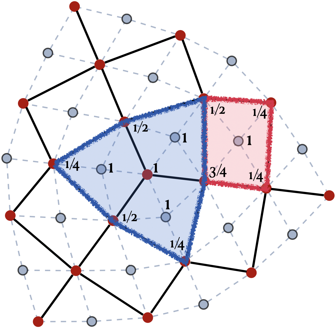
We construct a $\frac{\pi}{2}$ disclination at the point $o$ by deleting a quadrant from the infinite plane and reconnecting sites using the operator $\tilde{C}_{4,\lambda}$ (see Appendix C). In particular, if each unit cell in the disclination lattice has the same flux, we show that $\lambda_{o}=0$. Now consider a region $W$ enclosing the disclination, such that the distance between the disclination and the boundary $\partial W$ is much greater than the correlation length. The total charge is

where $n_{u.c.,W}$, $\Omega_{W}$ and $\delta\Phi_{W}$, are the number of unit cells in $W$, disclination angle, and excess magnetic flux (on top of the background flux $n_{u.c.,W}\phi$) respectively. Here we use that $\int_{W}dA=\delta\Phi_{W}+n_{u.c.,W}\phi$ and $\nu_{0}=C\phi/2\pi+k_{0}$. In order to use Eq. (2), $W$ should enclose a definite integer number of unit cells. Furthermore, in order to ensure that the condition $Q_{W}+Q_{W^{\prime}}=Q_{W\cup W^{\prime}}$ holds microscopically, as in the field theory, we define $Q_{W}\equiv\sum_{i\in W}\text{wt}(i)Q_{i}$ where the weight $\text{wt}(i)=1$ for interior points and $\text{wt}(i)=\frac{1}{4},\frac{2}{4},\frac{3}{4}$ if the interior of $W$ subtends an angle $\frac{\pi}{2},\pi,\frac{3\pi}{2}$ at site $i$ (see Fig. 2A. Lattice disclination with disclination angle = Ω π 2 . The blue region W covers 11 unit cells. Q i is weighted by the indicated amount when calculating Q W or ¯ Q W . B. Standard deviation of S as a function of bond disorder σ bond or onsite disorder σ onsite for = C 1 and = C 2 main Landau level (average hopping is 1). ). Note our definition of disclination charge differs from previous work. Li et al. 2020

The charge on a site $Q_{i}$ is simply $\expectationvalue{c_i^\dagger c_i}$ in the ground state. We choose $W$ such that it encloses a single disclination with $\Omega_{W}=\frac{\pi}{2}$. We set the excess flux $\delta\Phi_{W}=0$ in our numerics. $\nu_{0}$ can be defined as the filling of a corresponding clean lattice on a torus with the same flux per unit cell $\phi$. On a lattice with disclinations, $\nu_{0}$ is also the charge per unit cell far away from the disclination. Suppose we define the excess charge in $W$ as $\bar{Q}_{W}\equiv Q_{W}-\nu_{0}n_{u.c.,W}$. We can then extract the shift ${S}$ to be $\frac{{S}}{4}=\bar{Q}_{W}$. Numerically, we find that $\bar{Q}_{W}$, and hence the computed ${S}$ is indeed independent of the size of $W$ for large enough $W$. We show this by explicitly plotting $Q_{i}$ and the size dependence of $\bar{Q}_{W}$ for three representative sets of parameters in the Hofstadter butterfly (Fig. 3). We can thus use this procedure to calculate ${S}$ throughout the Hofstadter butterfly; this is shown in Fig. 1. In the Landau level limit, we numerically recover the result ${S}=\frac{C^{2}}{2}$ Wen and Zee 1992.

It is instructive to apply Eq. (2) when $W$ is the entire surface of a cube, which has 8 $\frac{\pi}{2}$ disclinations corresponding to the 8 corners. In this case, we obtain

Thus, in order to be in the same gapped phase as a state on a torus with filling $\nu_{0}$ and identical $\phi$ and Chern number $C$, the total charge on the cube is shifted from the naïve expectation of $\nu_{0}n_{u.c.,\text{cube}}$ by $2{S}$. Numerically, this agrees with the number of extra single particle states we need to fill.

Note that the weighting procedure and the numerical result $\bar{Q}_{W}=\frac{{S}}{4}$ generalize to any $C_{4}$ symmetric lattice. The details are described in Appendix E.

Let us now introduce bond and on-site potential disorder, which break the crystalline symmetry. In this case, the value of ${S}$ extracted from $\bar{Q}_{W}$ through ${S}=4\bar{Q}_{W}$ deviates from its quantized value for each disorder realization, although remains quantized after disorder averaging. The standard deviation $\sigma_{{S}}$ computed from $\bar{Q}_{W}$ grows to order 1 with an increase in disorder strength, as shown for two representative lobes in Fig.  2A. Lattice disclination with disclination angle = Ω π 2 . The blue region W covers 11 unit cells. Q i is weighted by the indicated amount when calculating Q W or ¯ Q W . B. Standard deviation of S as a function of bond disorder σ bond or onsite disorder σ onsite for = C 1 and = C 2 main Landau level (average hopping is 1). . The value of ${S}$ extracted from $Q_{\text{cube}}$ is much more robust (i.e. much smaller standard deviation) as long as the chemical potential is far from the band edge, since in this case $Q_{\text{cube}}$ can change only if a given disorder configuration moves a single particle state across the chemical potential.

Since $\omega$ is a rotation gauge field, the angular momentum is the charge under rotations, given by $l=\int\frac{\delta\mathcal{L}}{\delta\omega_{0}}={S}(\frac{\delta\Phi}{2\pi}+\frac{\phi}{2\pi}n_{u.c.})+k_{s}n_{u.c.}\mod 4$. Below we compare this topological field theory (TFT) prediction to microscopic calculations. Consider the Hofstadter Hamiltonian on an $L\times L$ torus, with $L$ even and $\phi$ flux per plaquette. By turning on $\delta A$, we add a flux $2\pi\Delta m$, also distributed uniformly. If the system has Chern number $C$, we fill $\Delta mC$ additional single particle states in order to get a gapped many body state with the same $C$. This state has $m=\frac{\phi L^{2}}{2\pi}+\Delta m$ flux quanta.

We use the same magnetic rotation operator $\tilde{C}_{4,\lambda}$ that we used to define the disclination. This means that we require $\lambda_{o}=0$, where $o$ is a fixed point of the rotation.

Note that the holonomies $e^{-i\oint(\delta A+A_{bgd})\cdot dl}$ along the two non-contractible cycles of the torus are position dependent. Translation by one site changes the holonomy by a factor $e^{i2\pi\frac{m}{L}}$, and is therefore an exact symmetry only for the infinite system; for any finite system, translation by one site can only be an approximate symmetry. On a finite size torus with even $L$, there are two points, $o_{1}$ and $o_{2}$, distinguished by having holonomy $1$ or $e^{i\pi m}$ along both directions. The vertex-centered $\pi/2$ rotational symmetry is only exact for a finite size system when $o_{1}$ and $o_{2}$ are both fixed points of this rotation.

Since we have two distinct fixed points $o_{1}$ and $o_{2}$, there are two distinct choices of gauge satisfying the above condition, either $\lambda_{o_{1}}=0$ and $\lambda_{o_{2}}=m\frac{\pi}{2}$, or $\lambda_{o_{2}}=0$ and $\lambda_{o_{1}}=-m\frac{\pi}{2}$. In what follows we pick the first choice, denoted $\tilde{C}_{4}$; the second is related by an overall $U(1)$ rotation $e^{-i\hat{N}m\frac{\pi}{2}}$, as will be discussed in Appendix F.

The many-body ground state $|\Psi_{m}\rangle$ satisfies $\tilde{C}_{4}\ket{\Psi_m}=e^{il(m)\frac{\pi}{2}}\ket{\Psi_m}$. Since $\tilde{C}_{4}^{4}=1$, $l(m)$ is an integer mod 4.

In this setup, we require each rotation center to be a vertex. On a torus, this forces $L$ to be even: if $L$ were odd, any rotation would leave two points invariant, one at a vertex, and the other at a plaquette center. If the rotation center was at a plaquette center, then the original $\tilde{C}_{4}$ rotation would be modified by a lattice translation. The associated eigenvalue would receive a contribution from the $A\wedge\vec{T}$ term in Eq. (Model and response theory.), which we do not wish to consider here. Indeed, the numerical result with plaquette centred rotations is not consistent with Fig. 1.

We find from direct numerical calculation:

The quadratic dependence on $m$ is beyond the TFT description; while it is well-known from the continuum Landau level problem, it has not been derived using effective field theory.⁴⁴ 4 Liu et al. 2019 accounted for the $m^{2}$ contribution in terms of the angular momentum of the electromagnetic field, however physically this term arises from the electron fluid itself. For a given lobe, $K(C,L)$ is an integer which does not depend on $m$, but does depend on $C$ and $L$. We can obtain ${S}$ by subtracting the quadratic term and taking the difference: ${S}=l(m+1)-l(m)-Cm-\frac{C}{2}\mod 4.$ For each lobe with a given $C$, the value of ${S}$ obtained from Eq. (4) matches the result using Eq. (3), confirming the expected duality.

Instead of inserting additional $\Delta m$ flux uniformly everywhere, we can insert it locally in a smaller region $W$ symmetrically around the rotation center. We find that the value of ${S}$ remains constant for different sizes of $W$, even in the limit when $W$ contains just 4 plaquettes (when $C$ is small enough).

We can also extract ${S}$ using partial rotations You et al. 2020; Shiozaki et al. 2017. That is, in a system with background flux $2\pi m_{0}$ we insert a local flux of $2\pi\Delta m$ in a region $W$, and we compute $\langle\Psi_{\Delta m,m_{0}}|\tilde{C}_{4}|_{D}|\Psi_{\Delta m,m_{0}}\rangle$, where $\tilde{C}_{4}|_{D}$ is the restriction of $\tilde{C}_{4}$ to a region $D$ containing $W$ and $|\Psi_{\Delta m,m_{0}}\rangle$ is the ground state. Let us fix $W$ and $D$ to be centered on $o_{2}$ and continue with our previous gauge choice $\lambda_{o_{1}}=0$. The ground state expectation value can be written as $\bra{\Psi_{\Delta m, m_0}}\tilde{C}_{4}|_{D}\ket{\Psi_{\Delta m, m_0}}=e^{-\gamma_{D}(\Delta m,m_{0})+il_{D}(\Delta m,m_{0})\pi/2}$. The magnitude $e^{-\gamma_{D}(\Delta m,m_{0})}$ has an exponentially decaying envelope as the perimeter $\partial D$ increases, as expected, in addition to an oscillatory behavior that we do not study in detail. We empirically find $l_{D}(\Delta m,m_{0})=l_{D}(0,m_{0})+{S}\Delta m+Cm\Delta m+\frac{C(\Delta m)^{2}}{2}\mod 4$. This matches the expectation from Eq. (4). One can also perform the partial rotation computation in the case where the total system is defined with open boundary conditions, as discussed in Appendix F.

On the torus we find that the formula for $l_{D}(\Delta m,m_{0})-l_{D}(0,m_{0})$ is sensitive in complicated ways to the gauge choice $\lambda_{o_{1}}=0$ or $\lambda_{o_{2}}=0$, and whether $D$ is centered on $o_{1}$ or $o_{2}$; these dependencies are not fully understood. We discuss this and related issues arising for open boundary conditions in Appendix F.

As a function of $\mu$ and $\phi$, ${S}$ and $C$ have the following general properties (note ${S}$ is defined $\mod 4$):

1. 1.

   ${S}\text{ mod }1=\frac{C}{2}\text{ mod 1}$.

2. 2.

   ${S}(\mu,\phi)={S}(\mu,2\pi-\phi)$, i.e. ${S}$ is invariant under time-reversal.

3. 3.

   For the bands with the same Chern number $C$, ${S}(\mu,\phi)=1-{S}(-\mu,\phi)$.

4. 4.

   When ${S}$ changes, $\frac{\phi}{2\pi}$ must lies in the Farey sequence of order $|C|$.

5. 5.

   ${S}(\mu,0^{+})=\frac{C^{2}}{2}$ for $C>0$.

Properties (1-3) will be justified in Appendix H. We explain (1) also for general interacting systems, using the classification of invertible topological phases in Ref. Barkeshli et al. 2021. (2) follows for general interacting systems from the time-reversal invariance of the field theory term $\omega\wedge dA$, while (5) reproduces the known results in the continuum Landau level limit Wen and Zee 1992.

Now let us explain property (4). Consider all possible fractions $\frac{p}{q}$ with $0\leq\frac{p}{q}\leq 1$, $1\leq q\leq 2|C|$ and $p,q$ coprime. Arrange them in increasing order, with 0 being the first element and 1 being the last. The resulting sequence is called the Farey sequence of order $2|C|$. Now, the different lobes with Chern number $C$ are uniquely specified by the intervals of $\frac{\phi}{2\pi}$ obtained from this sequence Osadchy and Avron 2001. Moreover, each lobe has a constant value of shift. In our numerics, when ${S}$ jumps, $\phi/2\pi$ must lie at fractions $\frac{p}{q}$ in a smaller set, namely the Farey sequence of order $|C|$: see Appendix B.

Suppose we fix a $C>0$ and consider ${S(\phi)}$ as $\frac{\phi}{2\pi}=\frac{p}{q}$ is increased from 0 to 1. As stated above, ${S}(\phi)$ jumps by integers at specific values of $\frac{p}{q}$, where $q\leq|C|$. At a given $\frac{p}{q}$, the total jump, defined as $\lim\limits_{\epsilon\rightarrow 0^{+}}{S}(2\pi\frac{p}{q}+\epsilon)-{S}(2\pi\frac{p}{q}-\epsilon)$, is the sum of two contributions: A contribution of $-C-1$ whenever $q$ divides $C$, and another contribution of $2\lfloor\frac{C+q}{2q}\rfloor$ whenever $q$ is odd. Both contributions are automatically 0 if $q>|C|$. The observed jumps are tabulated in Appendix B up to $C=12$. From these observations, we propose the following empirical formula by summing over all jumps that occur at $2\pi\frac{p}{q}<\phi$. For $C>0$,

where in the third term we sum over all $\frac{p}{q}$ in the Farey sequence of order $C$ that satisfy $\frac{p}{q}<\frac{\phi}{2\pi}$ and $q$ odd. ${S}$ for $C<0$ can be obtained from the symmetry transformation ${S}(\mu,\phi)=1-{S}(-\mu,\phi)$ which flips the sign of $C$. We numerically checked Eq. (5) for all $|C|\leq 7$ lobes using Eq. (3) on a cube of side length $L=28$. We also checked all $|C|\leq 12$ lobes using Eq. (4) on a torus with side length $L=140$, and we checked some representative $|C|=45$ lobes with $L=180$. We use (5), together with an eigenvalue database Osadchy and Avron 2001, to generate Fig. 1.

Lobes with the same $(C,k_{0})$ can have distinct values of ${S}$. For example when $(C,k_{0})=(4,-1)$ we can take $\frac{\phi}{2\pi}=1/3\mp\epsilon$, and find ${S}=3,1\mod 4$ respectively. Also note that in Fig. 1, we do not see any bands with total shift ${S}=3/2$ or 7/2. However, there is no theoretical obstruction to realizing this in a system with odd $C$. Indeed, there are several examples of single excited bands that have odd $C$ and ${S}=3/2$ or $7/2$ in this model.

We thank M. Hafezi and S. Das Sarma for comments on the draft, and V. Galitski and D. Bulmash for discussions on related projects. This work is supported by the Laboratory for Physical Sciences through the Condensed Matter Theory Center, NSF CAREER (DMR- 1753240) (MB, NM), ARO W911NF-20-1-0232 (GN).

References

- Wen and Zee (1992) X. G. Wen and A. Zee, Shift and spin vector: New topological quantum numbers for the hall fluids, Phys. Rev. Lett. 69, 953 (1992).
- Avron et al. (1995) J. E. Avron, R. Seiler, and P. G. Zograf, Viscosity of quantum hall fluids, Phys. Rev. Lett. 75, 697 (1995).
- Read (2009) N. Read, Non-abelian adiabatic statistics and hall viscosity in quantum hall states and paired superfluids, Phys. Rev. B 79, 045308 (2009).
- Read and Rezayi (2011) N. Read and E. H. Rezayi, Hall viscosity, orbital spin, and geometry: Paired superfluids and quantum hall systems, Phys. Rev. B 84, 085316 (2011).
- Haldane (2009) F. D. M. Haldane, ”hall viscosity” and intrinsic metric of incompressible fractional hall fluids (2009), arXiv:0906.1854 [cond-mat.str-el] .
- Haldane (2011) F. D. M. Haldane, Geometrical description of the fractional quantum hall effect, Phys. Rev. Lett. 107, 116801 (2011).
- Abanov and Gromov (2014) A. G. Abanov and A. Gromov, Electromagnetic and gravitational responses of two-dimensional noninteracting electrons in a background magnetic field, Phys. Rev. B 90, 014435 (2014).
- Bradlyn and Read (2015) B. Bradlyn and N. Read, Low-energy effective theory in the bulk for transport in a topological phase, Phys. Rev. B 91, 125303 (2015).
- Gromov et al. (2015) A. Gromov, G. Y. Cho, Y. You, A. G. Abanov, and E. Fradkin, Framing anomaly in the effective theory of the fractional quantum hall effect, Phys. Rev. Lett. 114, 016805 (2015).
- Schine et al. (2016) N. Schine, A. Ryou, A. Gromov, A. Sommer, and J. Simon, Synthetic landau levels for photons, Nature 534, 671 (2016).
- Wu et al. (2017) Y.-H. Wu, H.-H. Tu, and G. J. Sreejith, Fractional quantum hall states of bosons on cones, Phys. Rev. A 96, 033622 (2017).
- Manjunath and Barkeshli (2021) N. Manjunath and M. Barkeshli, Crystalline gauge fields and quantized discrete geometric response for abelian topological phases with lattice symmetry, Phys. Rev. Research 3, 013040 (2021).
- Manjunath and Barkeshli (2020) N. Manjunath and M. Barkeshli, Classification of fractional quantum hall states with spatial symmetries, arXiv preprint arXiv:2012.11603 (2020).
- Hofstadter (1976) D. R. Hofstadter, Energy levels and wave functions of bloch electrons in rational and irrational magnetic fields, Phys. Rev. B 14, 2239 (1976).
- Barkeshli et al. (2021) M. Barkeshli, Y.-A. Chen, P.-S. Hsin, and N. Manjunath, Classification of (2+1)d invertible fermionic topological phases with symmetry (2021), arXiv:2109.11039 [cond-mat.str-el] .
- Freed and Hopkins (2016) D. S. Freed and M. J. Hopkins, arXiv:1604.06527 (2016).
- Aasen et al. (2021) D. Aasen, P. Bonderson, and C. Knapp, Characterization and classification of fermionic symmetry enriched topological phases, (2021), arXiv:2109.10911 [cond-mat.str-el] .
- Dean et al. (2013) C. R. Dean et al., Hofstadter’s butterfly and the fractal quantum hall effect in moiré superlattices, Nature 497, 598 (2013).
- Hunt et al. (2013) B. Hunt et al., Massive dirac fermions and hofstadter butterfly in a van der waals heterostructure, Science 340, 1427 (2013).
- Saito et al. (2021) Y. Saito et al., Hofstadter subband ferromagnetism and symmetry-broken chern insulators in twisted bilayer graphene, Nature Physics 17, 478 (2021).
- Spanton et al. (2018) E. M. Spanton et al., Observation of fractional chern insulators in a van der waals heterostructure, Science 360, 62 (2018).
- Aidelsburger et al. (2013) M. Aidelsburger, M. Atala, M. Lohse, J. T. Barreiro, B. Paredes, and I. Bloch, Realization of the hofstadter hamiltonian with ultracold atoms in optical lattices, Phys. Rev. Lett. 111, 185301 (2013).
- Miyake et al. (2013) H. Miyake, G. A. Siviloglou, C. J. Kennedy, W. C. Burton, and W. Ketterle, Realizing the harper hamiltonian with laser-assisted tunneling in optical lattices, Phys. Rev. Lett. 111, 185302 (2013).
- Kennedy et al. (2015) C. J. Kennedy, W. C. Burton, W. C. Chung, and W. Ketterle, Observation of bose–einstein condensation in a strong synthetic magnetic field, Nature Physics 11, 859 (2015).
- Hafezi et al. (2013) M. Hafezi, S. Mittal, J. Fan, A. Migdall, and J. M. Taylor, Imaging topological edge states in silicon photonics, Nature Photonics 7, 1001 (2013).
- Ozawa et al. (2019) T. Ozawa, H. M. Price, A. Amo, N. Goldman, M. Hafezi, L. Lu, M. C. Rechtsman, D. Schuster, J. Simon, O. Zilberberg, and I. Carusotto, Topological photonics, Rev. Mod. Phys. 91, 015006 (2019).
- Biswas and Son (2016) R. R. Biswas and D. T. Son, Fractional charge and inter-landau–level states at points of singular curvature, Proceedings of the National Academy of Sciences 113, 8636 (2016).
- Liu et al. (2019) S. Liu, A. Vishwanath, and E. Khalaf, Shift insulators: Rotation-protected two-dimensional topological crystalline insulators, Phys. Rev. X 9, 031003 (2019).
- Li et al. (2020) T. Li, P. Zhu, W. A. Benalcazar, and T. L. Hughes, Fractional disclination charge in two-dimensional -symmetric topological crystalline insulators, Phys. Rev. B 101, 115115 (2020).
- You et al. (2020) Y. You, J. Bibo, and F. Pollmann, Higher-order entanglement and many-body invariants for higher-order topological phases, Phys. Rev. Research 2, 033192 (2020).
- May-Mann and Hughes (2021) J. May-Mann and T. L. Hughes, Crystalline responses for rotation-invariant higher-order topological insulators (2021), arXiv:2108.00008 .
- Peterson et al. (2021) C. W. Peterson, T. Li, W. Jiang, T. L. Hughes, and G. Bahl, Trapped fractional charges at bulk defects in topological insulators, Nature 589, 376 (2021).
- Han et al. (2019) B. Han, H. Wang, and P. Ye, Generalized wen-zee terms, Phys. Rev. B 99, 205120 (2019).
- Thouless et al. (1982) D. J. Thouless, M. Kohmoto, M. P. Nightingale, and M. den Nijs, Phys. Rev. Lett. 49, 405 (1982).
- Osadchy and Avron (2001) D. Osadchy and J. E. Avron, Hofstadter butterfly as quantum phase diagram, Journal of Mathematical Physics 42, 5665 (2001), https://doi.org/10.1063/1.1412464 .
- Shiozaki et al. (2017) K. Shiozaki, H. Shapourian, and S. Ryu, Many-body topological invariants in fermionic symmetry-protected topological phases: Cases of point group symmetries, Phys. Rev. B 95, 205139 (2017).
- Barkeshli et al. (2019) M. Barkeshli, P. Bonderson, M. Cheng, and Z. Wang, Symmetry fractionalization, defects, and gauging of topological phases, Phys. Rev. B 100, 115147 (2019).
- Kapustin (2014) A. Kapustin, Bosonic topological insulators and paramagnets: a view from cobordisms, (2014), arXiv:1404.6659 .
- Witten (1989) E. Witten, Quantum field theory and the Jones polynomial, Comm. Math. Phys. 121, 351 (1989).
- Thorngren and Else (2018) R. Thorngren and D. V. Else, Gauging spatial symmetries and the classification of topological crystalline phases, Phys. Rev. X 8, 011040 (2018).
- Debray (2021) A. Debray, Invertible phases for mixed spatial symmetries and the fermionic crystalline equivalence principle (2021), arXiv:2102.02941 [math-ph] .
- Wang and Gu (2020) Q.-R. Wang and Z.-C. Gu, Construction and classification of symmetry-protected topological phases in interacting fermion systems, Phys. Rev. X 10, 031055 (2020).
- Else and Thorngren (2019) D. V. Else and R. Thorngren, Crystalline topological phases as defect networks, Phys. Rev. B 99, 115116 (2019).
- Zhang et al. (2020) J.-H. Zhang, S. Yang, Y. Qi, and Z.-C. Gu, Real-space construction of crystalline topological superconductors and insulators in 2d interacting fermionic systems, (2020), arXiv:2012.15657 [cond-mat.str-el] .
Appendix A Relation to prior work
Here we summarize how our results relate to those in several prior works where the physical manifestation of the Wen-Zee shift is studied in a lattice setting.
Our contributions include:
- 1.
A method to unambiguously extract the discrete shift by computing the charge in a region containing a disclination, or through the angular momentum . Crucially, one must use the same rotation operator to define the disclination Hamiltonian and to compute the angular momentum. An important ingredient in our formula which was not introduced previously is the fractional weighting for sites on the boundary . This fractional weighting is crucial to obtaining a simple formula that matches the topological field theory result.
- 2.
We have shown that the shift is a half-integer defined modulo in the case of -fold rotational symmetry, and that is half-integer or integer depending on whether is odd or even, and we have derived these statements even in the case of interacting fermions.
- 3.
We have also provided an empirical formula for everywhere in the Hofstadter butterfly for the square lattice Hofstadter model.
Ref. Liu et al. 2019 discusses disclination charge in a model on the honeycomb lattice with rotational symmetry and particle-hole symmetry in the absence of a background magnetic field. They exploited the particle-hole symmetry to derive an analytical formula for disclination charge, and therefore the shift. We studied the disclination charge on the square lattice numerically in the presence of a background magnetic field (allowing for a tunable Chern number). In order to do so, we arrived at the prescription that allows us to isolate the shift, given a very general charge distribution in a state.
Ref. Liu et al. 2019 also studied the angular momentum response using global plaquette centered rotations. We note that in our case, i.e., for 4-fold rotational symmetries, there exist both vertex- and plaquette-centred rotations, which are related to each other by a lattice translation; the latter may also introduce contributions from the field theory term . However, the model considered in Ref. Liu et al. 2019 has only plaquette rotation centers, so this distinction does not arise in their case. The extra field theory term is also expected to be trivial for systems with -fold rotational symmetry Manjunath and Barkeshli 2021; Manjunath and Barkeshli 2020. We also note that gauge transformations required to accompany the rotation operator are nontrivial on the square lattice, because we cannot use a symmetric gauge (w.r.t. a vertex rotation center) to insert flux. But this is not an issue in Ref. Liu et al. 2019, as a symmetric gauge can be used for symmetric lattices, in which case the rotation operator does not require any additional gauge transformations.
Ref. Biswas and Son 2016 also performs a disclination charge calculation for Landau levels in detail, especially studying the contributions from inter-LL states. The analytical derivations of disclination charge are done in the continuum limit, and numerically verified for lattice systems. The calculations are all performed on closed surfaces with corners, so that the charge of a single disclination is deduced by symmetry, analogous to the results discussed in this paper. This work is effectively restricted to parts of the Hofstadter butterfly that reduce to Landau levels in the continuum limit.
Ref. Li et al. 2020 derives a formula for disclination charge when Chern number , in terms of the charge distribution at high-symmetry points of the unit cell. Their definition of disclination charge is distinct from ours. In the symmetric case, it is equivalent to choosing a region in the dual lattice, and evaluating for this as we have outlined. If we denote their disclination charge result as , we find that for symmetric lattices with zero Chern number. We note that our definition of disclination charge, with defined on the physical lattice, is directly proportional to , which also agrees with the coefficient of the linear contribution to the angular momentum associated to vertex-centred rotations. In this sense as defined in the main text is more directly related to the Wen-Zee coefficient and the prediction from the topological field theory.
In the case, Ref. Li et al. 2020 writes down the Wen-Zee term with for specific models. It also proposes a formula for disclination charge in the case, in terms of band invariants at high-symmetry points of the Brillouin zone. The values of disclination charge from this definition are different from ours, although we have not studied this relationship in detail when . This paper does not make an explicit connection between this formula and the Wen-Zee coefficient . In our work we have shown that , which is proportional to , depends sensitively on the Chern number through the relation .
In related work, Ref. May-Mann and Hughes 2021 discussed a spinless fermion system on the square lattice with , and calculated the fractional charge bound to a disclination at half filling. Finally, Refs. Shiozaki et al. 2017; You et al. 2020 study the angular momentum response using partial rotations in bosonic and fermionic models respectively. The specific models studied numerically have Chern number .
Appendix B Jumps of
In this section we tabulate the data used to empirically obtain Eq.(5) in the main text. Starting from the zero-flux value , Fig. 4 shows how jumps as is increased keeping fixed. The Hofstadter lobes corresponding to Chern number are separated by the Farey sequence of order . But from the figure, we see that only jumps at fractions lying in the Farey sequence of order , which is a smaller set. We have confirmed this up to , see Fig. 4. For example, at , the Farey sequence of order 8 is , with the rest of the sequence obtained by reflecting about . However, only jumps at , all of which lie in the Farey sequence of order 4.
Appendix C Definition of disclination Hamiltonian using
In this section we first define on the infinite plane; is fixed up to a constant by the background vector potential , where is the rotation center. We then construct a disclination Hamiltonian by removing a quadrant and connecting the open edges by defining new hopping terms. This is essentially an adaptation of the prescription to construct symmetry defects for on-site symmetries given in Ref. Barkeshli et al. 2019. The values of the new hopping terms are determined by . We show that requiring the disclination to not insert any additional flux, fixes . For a fixed on the infinite plane, this completely fixes .
C.1 Definition of and on an infinite plane
We define the rotation operator on the infinite plane as