Focal Length and Object Pose Estimation via Render and Compare
Abstract
We introduce FocalPose, a neural render-and-compare method for jointly estimating the camera-object 6D pose and camera focal length given a single RGB input image depicting a known object. The contributions of this work are twofold. First, we derive a focal length update rule that extends an existing state-of-the-art render-and-compare 6D pose estimator to address the joint estimation task. Second, we investigate several different loss functions for jointly estimating the object pose and focal length. We find that a combination of direct focal length regression with a reprojection loss disentangling the contribution of translation, rotation, and focal length leads to improved results. We show results on three challenging benchmark datasets that depict known 3D models in uncontrolled settings. We demonstrate that our focal length and 6D pose estimates have lower error than the existing state-of-the-art methods.
1 Introduction
The projection of a 3D object into an image depends not only on the object’s relative pose to the camera, but also on the camera’s intrinsic parameters. While it is possible to capture objects in a controlled environment where the camera’s intrinsic parameters are known (e.g., a calibrated camera on a robot), for many “in-the-wild” images we do not have control over the capture process and these parameters are unknown, e.g., Internet pictures or archival photographs.


Given an input image, we seek to retrieve a 3D model of a depicted object from a model library and estimate the relative camera-object 6D pose jointly with the camera’s focal length (depicted in Figure 1). This problem has its origins in the early days of computer vision Lowe1999-bf; Lowe1987-yf; Roberts1963-ck and has important modern-day applications in augmented reality and computer graphics, such as applying in situ object overlays or editing the position of an object via 3D compositing in uncontrolled consumer-captured images.
The problem of 6D object pose estimation in an uncalibrated setting is, by its nature, challenging. First, it is difficult to distinguish subtle changes of the camera’s focal length from changes in an object’s depth. Second, including the camera’s focal length increases the number of parameters that must be estimated and hence increases the optimization complexity. Finally, “in-the-wild” consumer-captured images may depict large appearance variation for a particular object instance in the model library. Variation may be due to differences in illumination and the depicted object having slightly different, non-identical shapes or surface appearance in different real-world instance captures. For example, consider different instances of the same car model that have a similar overall shape but may have different color, wear and tear, or customizable features (e.g., additional headlights, alloy wheels, or a spoiler).
Previous approaches for this task primarily rely on establishing local 2D-3D correspondences between an image and a 3D model using either hand-crafted Aubry14; bay2006surf; Collet2010-zj; Collet2011-lj; Hinterstoisser2011-es; Lowe1999-bf or CNN features grabner2019gp2c; hu2019segmentation; Kehl2017-ek; Park2019-od; pavlakos20176; peng2019pvnet; Rad2017-de; song2020hybridpose; Tekin2017-hp; Tremblay2018-bd; Xiang2018-dv; zakharov2019dpod, followed by robust camera pose estimation using PnP lepetit2009epnp. These approaches often fail on scenes with large textureless areas where local correspondences cannot be reliably established. In contrast, the recent best-performing 6D object pose estimation methods are based on the render-and-compare strategy labbe2020cosypose; li2018deepim; manhardt2018deep; oberweger2019generalized; zakharov2019dpod, which performs a dense alignment over all pixels of rendered views of the 3D model to its depiction in the input image. However, all prior render-and-compare methods fall short of handling the aforementioned desired uncontrolled, uncalibrated setting as they assume a controlled environment where the camera intrinsic parameters are fixed and known a priori. Also, these prior methods typically operate over only a handful of known objects.
To address these challenges, we build on the strengths of render and compare and extend it to handle our desired uncontrolled, uncalibrated setting. We introduce FocalPose, a novel render-and-compare approach for jointly estimating an object’s 6D pose and camera focal length based on a monocular image input. Our contributions are twofold. First, we extend a recent state-of-the-art hodan2020bop method for 6D pose estimation (CosyPose labbe2020cosypose) by deriving and integrating focal length update rules in a differentiable manner, which allows our method to overcome the added complexity of including the focal length. Second, we investigate several different loss functions for jointly estimating object pose and focal length. We find that a combination of direct focal length regression with a reprojection loss disentangling the contribution of translation, rotation, and focal length leads to the best performance and allows our method to distinguish subtle differences due to the focal length and the object’s depth. We apply our method to three real-world consumer-captured image datasets with varying camera focal lengths and show that our focal length and 6D pose estimates have lower error compared to the state of the art. As an added benefit, our work is the first render-and-compare method applied to a large collection of 3D meshes (20-200 meshes for Pix3D pix3d, for the car datasets wang20183d).
2 Related Work
6D pose estimation of rigid objects from RGB images.
This task is one of the oldest problems in computer vision Roberts1963-ck; Lowe1987-yf; Lowe1999-bf and has been successfully approached by estimating the pose from 2D-3D correspondences obtained via local invariant features Lowe1999-bf; bay2006surf; Collet2010-zj; Collet2011-lj, or by template-matching Hinterstoisser2011-es. Both of these strategies rely on shallow hand-designed image features and have been revisited with learnable deep convolutional neural networks (CNNs) Rad2017-de; Tremblay2018-bd; Kehl2017-ek; Tekin2017-hp; peng2019pvnet; pavlakos20176; hu2019segmentation; Xiang2018-dv; Park2019-od; song2020hybridpose; zakharov2019dpod. The best-performing methods for 6D pose estimation from RGB images are now based on variants of the deep render-and-compare strategy li2018deepim; manhardt2018deep; oberweger2019generalized; labbe2020cosypose; zakharov2019dpod. However, these methods assume the full perspective camera model is known so that the object can be rendered and compared with the input image. We build on the state-of-the-art render-and-compare approach of Labbé et al. labbe2020cosypose and extend it to the “in-the-wild” uncontrolled set-up where the focal length of the camera is not known and has to be estimated together with the object’s 6D pose directly from the input image.
Camera calibration.
Camera calibration techniques faugeras1993three; andrew2001multiple; nakano2016versatile; penate2013exhaustive; zheng2014general; tsai1987versatile; dubska2014fully; szeliski2010computer recover the camera model (intrinsic parameters) and its pose (extrinsic parameters) jointly. A limitation is that they require estimating 2D-3D correspondences in multiple images using structured object patterns Forsyth12; Hartley2004; szeliski2010computer; tsai1987versatile, identifying specific image elements such as lines or vanishing points dubska2014fully; chen2004camera; szeliski2010computer or structured features (e.g., human face landmarks burgos2014distance). These requirements limit their applicability to unconstrained images where these structures are not present. Other works workman2015deepfocal have considered in-the-wild images, but only focus on recovering the focal length of the camera. In contrast, our approach recovers both components of the camera calibration (focal length and 6D camera pose) given a single image of a known object.

(a)
 (b)
(b)
Joint 6D pose and focal length estimation from a single in-the-wild image.
The prior work closest to our approach establishes point correspondences, followed by robust fitting of the camera model wang20183d; grabner2019gp2c; han2020gcvnet. Wang et al. wang20183d uses Faster R-CNN with a scalar regression head and L1 loss for estimating the focal length, and the 6D pose is estimated by predicting 2D-3D correspondences followed by PnP.
GP2C grabner2019gp2c extends this approach via a two-step procedure that predicts initial 2D-3D correspondences and focal length with a similar direct regression, followed by applying a PnPf solver to refine jointly the 6D pose and the focal length. The model cannot be trained end-to-end as it relies on a separate non-differentiable optimizer. GCVNet han2020gcvnet uses an approximation of the PnPf solver for differentiability, but its results are limited by this approximation. In contrast, our work builds on the success of the recent render-and-compare methods labbe2020cosypose; li2018deepim for 6D rigid pose estimation. Our 6D pose and focal length updates are learned end-to-end using our novel focal length update parameterization coupled with a disentangled training loss. Our approach produces lower-error focal length and pose estimates compared to the two-step approach of GP2C grabner2019gp2c and the prior one-shot end-to-end approaches wang20183d; han2020gcvnet.
3 Approach
Our goal is to estimate the 6D pose of objects in a photograph taken with unknown focal length. To achieve this goal, we use a render-and-compare strategy where we estimate jointly the camera focal length with the 6D pose. We assume knowledge of a database of 3D models that may appear in the image, but our results show that the approach is effective even if the 3D models are only approximate.
3.1 Approach Overview
The first step of our approach, illustrated in Fig. 2, identifies the object location in the input image and retrieves a 3D model from the database that matches the depicted object instance. We use an object detector he_2017_iccv trained on real images of these known objects. At test time, we run this detector on the test image to obtain a 2D bounding box of the object and its corresponding 3D model . We describe a render and compare approach, which iteratively estimates the focal length and 6D pose of the identified object. We denote the current estimate of focal length and 6D pose at iteration jointly as . The object model is first rendered using the current estimates into an image using a renderer . The rendering and observed input image are given to a deep neural network which predicts the pose and focal length update :
| (1) |
The intuition is that the neural network compares the input image with the rendering and based on their (potentially subtle) differences predicts the update in the rendering parameters . The pose and focal length updates are designed to be, as much as possible, free of non-linearities and thus easy to predict by the neural network . The pose and focal length at the next iteration is then computed by a non-linear update rule :
| (2) |
where is the current estimate of the pose and focal length, is the prediction by the network given by eq. (1), and are the updated pose and focal length. Note that is not learnt but derived from the 3D to 2D projection model and takes into account the nonlinearities of the imaging process. The neural network is trained in such a way that the updated pose and focal length are progressively closer to their ground truth. Our approach is summarized in Fig. 2
Discussion.
Existing render-and-compare estimators labbe2020cosypose; li2018deepim require knowledge of the camera intrinsic parameters. In our scenario, the problem is more challenging because the rendering also depends on the unknown focal length. We address this challenge by proposing an update rule for the focal length as well as a modification of the update rules for 6D pose parameters accounting for the unknown focal length (Sec 3.2). We then introduce a novel loss function adapted for joint focal length and 6D pose estimation, which disentangles the effects of the pose and focal length updates for better end-to-end training of the network (Sec. 3.3). Please see the supp. materials for details of our implementation, parameter initialization, and our training data.
3.2 Update rules with focal length estimation
The standard render-and-compare approach to 6D pose estimation li2018deepim; labbe2020cosypose considers only translation and rotation as parameters . We additionally estimate the focal length as an unknown, and thus need to build an appropriate rule (as defined in eq. (2)) for updating jointly all parameters. In detail, we assume a pinhole camera model with focal length in which the optical center is set at the center of the image. We define the 6D pose of the object with respect to the camera by a 3D rotation and a 3D translation . Next, we describe our updates for focal length and 6D pose.
Focal length update.
To build an appropriate focal length update rule, we take into account the fact that it should remain strictly positive throughout the update iterations. We consider update rules that are multiplicative, i.e., they scale an initial guess by a sequence of multiplications. Let be the current estimate of the focal length at iteration and be the focal length update predicted by the network (see eq. (1)). We define the updated focal length as the multiplication,
| (3) |
The sequence of multiplicative updates can be written as , where is the initial focal length and are the individual updates. An alternative to the above strategy would be enforcing positivity of the focal length update via a sigmoid function instead of an exponential function. We found the exponential and sigmoid functions to behave similarly, but the sigmoid update requires setting an additional scale parameter. Hence, we opted for the simpler exponential updates as described in eq. (3).
6D pose update.
For the update of the 6D pose, we build on the update rule introduced in DeepIM li2018deepim that disentangles 3D rotation and 3D translation updates. In more detail, the network is trained to predict a translation of the projected object center into the image (measured in pixels), and a ratio of the camera-to-object depth between the observed and the rendered image. The 3D translation of the object is then updated from the quantities predicted by network , taking into account the nonlinear projection equations derived from the camera model. In li2018deepim the focal length is known and fixed. In our scenario the focal length is not fixed and we replace the known fixed focal length with the predicted focal length . In detail, the updated 3D translation of the object with respect to the camera is obtained as :
| (4) | ||||
| (5) | ||||
| (6) |
where are the object translation updates predicted by network as part of (eq. 1), is the 3D translation vector of the relative camera-object pose at iteration , is the new updated 3D translation vector, and is the updated focal length of the camera given by eq. (3).
To obtain the update of the rotation component of the object pose we use directly the prediction of the alignment network in a multiplicative update, which does not depend on the focal length. In particular, we parametrize the rotation update using two 3-vectors , that define the rotation matrix by Gram-Schmidt orthogonalization as described in Zhou2018-eg. This parametrization was found to work well for different prediction tasks Zhou2018-eg including 6D object pose estimation labbe2020cosypose. The resulting update rule is then written as
| (7) |
where is the new updated object rotation, is the current object rotation, and is the rotation matrix obtained by Gram-Schmidt orthogonalization from the two 3-vectors , predicted by the alignment network as part of . Note that this rotation update is similar to the one used in DeepIM li2018deepim.
3.3 Pose and focal length training loss
We now present our network training loss, where we assume the training data consist of image and aligned model pairs. Note that a training pair may be a real image with a manually aligned model or a rendered image of a model under a specified 6D pose and focal length. Given input parameters , the output parameters are fully defined by the network outputs given by eq. (1) and the differentiable update rules described by eqs. (3)-(7) in the previous section. In the following, we consider a single network iteration and denote as the estimated parameters. For jointly learning to estimate the 6D pose and the focal length, we use the following loss that penalizes errors in the output 6D pose predictions and the estimated focal length :
| (8) |
where are the estimated pose and focal length parameters, are the ground truth pose and focal length parameters, is a loss that penalizes errors in the 6D pose estimate, is our novel loss function that jointly takes into account the errors in the focal length and the 6D predicted pose, and is a scalar hyper-parameter. This loss is written for a single instance, but our model is trained to minimize the average loss over all training images. We now describe the individual losses and .
Focal length loss.
We use the following focal length loss:
| (9) |
where is Huber regression loss, is disentangled reprojection loss and is a scalar hyper-parameter. The individual terms are explained next. The Huber regression loss measures the errors between the estimated and the ground truth focal length using a logarithmic parametrization of the focal length following the recommendations from Grabner et al. grabner2019gp2c for better training:
| (10) |
where again is the ground truth focal length and is the focal length estimated by our model.
While using only the loss is possible for training our model, we found better results are obtained by also considering the 2D errors of the projected 3D model in the image using the current estimates of the focal length and object 6D pose. We first define the reprojection error:
| (11) |
where is the intrinsic camera matrix of our camera model with focal length , are 3D points sampled on the object model, is the projection of a 3D point using the current estimates of all the parameters, and is the projection of the same 3D point using ground truth parameters. This loss can be seen as the counterpart of the pose loss (defined below): instead of penalizing errors in 3D space, it penalizes reprojection errors in the image while also taking into account the estimated focal length . However, this loss does not disentangle the effects of the pose and focal length predictions. We thus introduce our disentangled reprojection loss:
| (12) | ||||
| (13) |
where each term separately measures the 2D reprojection errors resulting from errors in the 6D pose (the first term) and in the focal length (the second term). This disentanglement leads to faster convergence and better model accuracy, as we show in our ablation results.
6D pose loss.
For (in equation (8)), we build on the loss used in CosyPose labbe2020cosypose. This loss is based on the point-matching loss Xiang2018-dv; li2018deepim that measures the error between the alignment of the points on the 3D model transformed with the predicted pose and the ground truth pose . CosyPose labbe2020cosypose extends this loss to take into account object symmetries, and uses the disentanglement ideas of Simonelli2019-da to separate the influence of translation errors along the camera axis, image plane, and rotations. In our approach, we do not consider object symmetries as they are nontrivial to obtain for 3D models in the wild considered in this work. In detail, for the pose loss we utilize the following distance metric between two poses specified by and :
| (14) |
where denotes norm, is a rotation matrix, is a translation vector and is a point sampled from the mesh . Following labbe2020cosypose, we disentangle the pose loss as
| (15) | ||||
where are the pose and focal length parameters at iteration , is a ground truth rotation, is a ground truth translation, is a distance defined by Eq. (14) and is an update function defined by (2). The main idea of this loss is to separate the influence of translation errors in the plane, depth alignment errors along the axis, and rotation errors. In Eq. (15) the terms , and represent the necessary updates that lead to such loss disentanglement. Here are translation updates at iteration as predicted by the network , is a rotation update at iteration predicted by network and is a focal length update at iteration . and then represent the updates needed to transform the current parameters to the ground truth values, which leads to the disentanglement along each of the dimensions. The first term in Eq. (15) leads to the disentanglement along the axis, since this term provides the gradients resulting from the alignment errors. Analogously, the second and third terms provide gradients that arise from depth and rotation alignment errors.
4 Experiments
We evaluate our method for focal length and 6D pose estimation on three challenging benchmarks: the Pix3D pix3d, CompCars wang20183d and StanfordCars wang20183d datasets. In the remainder of this section we first introduce the benchmark datasets and give details of the full pose estimation pipeline. Then, in Sec. 4.1 we present the ablation of the main components of the proposed loss function. In Sec. 4.2 we compare our method with the state of the art wang2018improving; grabner2019gp2c; han2020gcvnet addressing the same task. Finally, in Sec. 4.3 we discuss the main limitations of our approach.
Datasets and evaluation criteria.
We consider three real-world in-the-wild datasets depicting objects with known 3D models annotated with ground truth focal length and 6D pose of the object. Following Grabner et al. grabner2019gp2c, we consider the bed, chair, sofa, and table classes in the Pix3D dataset pix3d. The images for each object class are considered as separate datasets. The Stanford cars and CompCars datasets wang20183d contain images of different car instances. Note that for the Pix3D chair images and both cars datasets, there are hundreds of different object instances in the dataset, which makes the task of recognizing the object instance challenging. We use the standard set of evaluation criteria used by prior work wang2018improving; grabner2019gp2c; han2020gcvnet that include the detection accuracy and several 6D pose metrics. The results are reported as median errors (smaller is better) between the prediction and ground truth (e.g., the is the median rotation error) and accuracies (higher is better), which report the percentage of images with an error smaller than a certain threshold (e.g., reports the percentage of test images with the rotation error smaller than ). See the supplemental for a detailed description of all the evaluation criteria.
The complete pose estimation pipeline.
The first step of our pipeline returns bounding box coordinates for depicted model instances in the input image via a Mask R-CNN detector. One detector is trained for each object class. For each detected instance, we crop the input image given the bounding box and apply an instance classifier to obtain which 3D model instance to align. In our case we finetune the DINO model caron2021emerging as the instance classifier. We align the 3D model instance corresponding to the top classifier score. The classifier achieves top-1 retrieval accuracy of 62.1% for Pix3D, 71.2% for Stanford Cars and 79.0% for CompCars datasets. Next, we estimate the coarse 6D pose and focal length using the full image, bounding box, and retrieved 3D model instance. Finally, the refiner FocalPose model iteratively refines the estimates for iterations given the coarse estimates.
4.1 Loss ablation study
In this section we ablate the different components of our proposed loss function. We train the coarse and refinement networks with the three different losses introduced in Section 3.3. We report the results in Table 1. First, our solution (c.) combining the Huber regression loss with the 2D reprojection error taking into account the object 3D model and its 6D pose results in significantly lower errors than simply using the regression loss (a.) used in Grabner et al. grabner2019gp2c. Second, our new loss (c.), which disentangles the effects of focal length and pose, results in lower median errors compared to the standard reprojection loss that does not disentangle pose and focal length (b.).
| Loss | |||
|---|---|---|---|
| a. | 6.61 | 1.51 | 4.17 |
| b. | 3.28 | 1.42 | 1.45 |
| c. | 2.98 | 1.29 | 1.36 |
4.2 Comparison to the state-of-the-art
Below we report the results of our approach on the three different datasets and compare with other methods for 6D object pose and focal length estimation wang2018improving; grabner2019gp2c; han2020gcvnet.
Pix3D dataset.
We report the average for the four classes (bed, chair, sofa, table) in Table 2 (top). The per-class results are in the supplementary material. On average over all classes, our method significantly outperforms the other methods in 5 out of the 8 metrics. In particular, we see a clear improvement in the estimated focal length (almost 11% relative reduction in the median focal length error, from 0.172 to 0.155). We see also a clear improvement in the estimated 3D translation (20% relative reduction in the median 3D translation error, from 0.185 to 0.148). Please note that the 3D translation is related to the focal length because of the focal length/depth ambiguity. These improvements are significant and validate the contribution of our method.
CompCars and Stanford cars.
A similar pattern of results is shown in Table 2 (middle, bottom) also for the CompCars and Stanford cars datasets that contain hundreds of different car models. Our approach obtains the best results in 4 (CompCars) and 5 (Stanford cars) of the 8 reported metrics. In particular, our method significantly improves the focal length estimates (11% relative reduction on CompCars and 54% relative reduction on Stanford cars) and the 3D translation estimates (10% relative reduction on CompCars and 52% relative reduction on StanfordCars). Again, these improvements are significant and validate the contribution of our method.
| Detection | Rotation | Translation | Pose | Focal | Projection | |||||
| Method | Dataset | |||||||||
| wang20183d | Pix3D | 96.0% | 7.25 | 87.8% | 2.52 | 1.76 | 2.41 | 6.33 | 71.5% | |
| grabner2019gp2c-LF | 96.2% | 6.92 | 88.4% | 1.85 | 1.30 | 1.72 | 3.85 | 85.5% | ||
| grabner2019gp2c-BB | 97.7% | 6.89 | 90.8% | 1.94 | 1.30 | 1.75 | 3.66 | 88.0% | ||
| Ours | 95.5% | 4.92 | 84.1% | 1.49 | 1.09 | 1.53 | 2.97 | 79.2% | ||
| wang20183d | CompCars | 98.9% | 5.24 | 97.6% | 3.30 | 2.35 | 3.23 | 7.85 | 73.7% | |
| grabner2019gp2c-LF | 98.8% | 5.23 | 97.9% | 2.61 | 1.86 | 2.97 | 4.21 | 95.1% | ||
| grabner2019gp2c-BB | 98.9% | 4.87 | 98.1% | 2.55 | 1.84 | 2.95 | 3.87 | 95.7% | ||
| han2020gcvnet-TwoStep | - | 4.37 | 98.1% | 3.22 | 1.90 | 3.79 | 4.54 | 90.2% | ||
| han2020gcvnet-GCVNet | - | 3.99 | 98.4% | 3.18 | 1.89 | 3.76 | 4.31 | 90.5% | ||
| Ours | 98.2% | 3.99 | 98.4% | 2.35 | 1.67 | 2.65 | 2.95 | 93.0% | ||
| wang20183d | Stanford | 99.6% | 5.43 | 98.0% | 2.33 | 1.80 | 2.34 | 7.46 | 76.4% | |
| grabner2019gp2c-LF | 99.6% | 5.38 | 98.3% | 1.93 | 1.51 | 2.01 | 3.72 | 96.2% | ||
| grabner2019gp2c-BB | 99.6% | 5.24 | 98.3% | 1.92 | 1.47 | 2.07 | 3.25 | 96.5% | ||
| han2020gcvnet-TwoStep | - | 5.09 | 97.5% | 2.29 | 1.52 | 2.52 | 3.78 | 93.6% | ||
| han2020gcvnet-GCVNet | - | 4.92 | 97.5% | 2.20 | 1.46 | 2.43 | 3.65 | 94.6% | ||
| Ours | 99.5% | 4.44 | 95.1% | 1.00 | 0.84 | 1.09 | 2.55 | 93.8% | ||
a
Input image
 Ground truth
 Our prediction

b


c


Qualitative results.
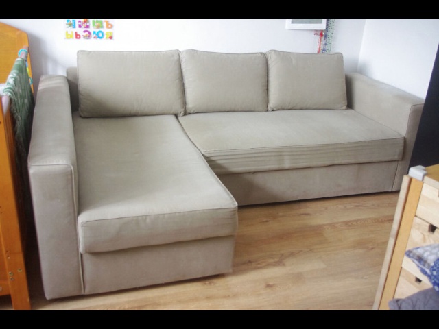
We report examples of qualitative results for our method on the four classes of the Pix3D dataset in Fig. 4 and qualitative results on Stanford cars and CompCars datasets in Fig. 5. Please note that the renderings of the predictions (taking into account focal length and object 6D pose) show precise alignment with the observed image for in-the-wild photographs. Notably, these qualitative results demonstrate the robustness of our approach to large object truncation and strong perspective effects. Please see the supplementary material for additional qualitative results and comparisons.
1
Input image
 Ground truth
 Our prediction

2


3


4


5


6


7


8


9


1
Input image
 Ground truth
 Our prediction

2


3


4


5


6


7


8


4.3 Limitations
There are three main failure modes of our approach, illustrated in Fig. 3. First, we observe high rotation errors for symmetric objects such as tables or stools, where the correct orientation is ambiguous. Please note that none of the used evaluation criteria take into account the symmetries of objects. Second, our iterative alignment procedure can get stuck into a local minima where the predicted object model in the predicted configuration is reasonably aligned but the errors are still high, e.g., because the object is flipped upside down. This failure could be mitigated by running our approach from multiple initializations or running our refinement network on better coarse estimates. Finally, we observe that in some situations the 3D model retrieved by our pipeline is incorrect. These failure modes lead to large errors, which explains the lower accuracies measured by the and metrics. Nevertheless, our approach achieves significantly lower median errors (5 out of the 8 reported metrics) compared to the current state-of-the-art methods, which demonstrates the high precision of our approach outside of these failure modes.
Broader impact. Our work has the potential to positively impact practical applications in augmented reality and robotics, among them overlaying artistic effects on viewed objects or for a robotic assistant that can manipulate real-world objects. However, our work could also potentially be used as a component for 3D-assisted manipulation of an image or video via object compositing to create misinformation.
5 Conclusion
We have demonstrated successful joint estimation of camera-object 6D pose and camera focal length given a single still image. Key to our success was our extension of render and compare that incorporated the estimated focal length in the iterative update rules and a disentangled loss for training. We have shown that our approach produces lower-error focal length and pose estimates compared to prior art.
Our approach can be extended to other camera intrinsic parameters besides focal length, including different forms of camera distortions, provided they can be reliably rendered. This work opens up the possibility of downstream applications in augmented reality/computer graphics and reasoning over “in-the-wild” articulated and interacted objects in video.
Acknowledgements.
This work was partly supported by the European Regional Development Fund under the project IMPACT (reg. no. CZ.02.1.01/0.0/0.0/15_003/0000468), the Ministry of Education, Youth and Sports of the Czech Republic through the e-INFRA CZ (ID:90140), the French government under management of Agence Nationale de la Recherche as part of the “Investissements d’avenir” program, reference ANR19-P3IA-0001 (PRAIRIE 3IA Institute).
References
- (1) Alex M Andrew. Multiple view geometry in computer vision. Kybernetes, 2001.
- (2) Mathieu Aubry, Daniel Maturana, Alexei Efros, Bryan Russell, and Josef Sivic. Seeing 3D chairs: exemplar part-based 2D-3D alignment using a large dataset of CAD models. In CVPR, 2014.
- (3) Herbert Bay, Tinne Tuytelaars, and Luc Van Gool. Surf: Speeded up robust features. In ECCV, pages 404–417. Springer, 2006.
- (4) Xavier P Burgos-Artizzu, Matteo Ruggero Ronchi, and Pietro Perona. Distance estimation of an unknown person from a portrait. In ECCV, pages 313–327. Springer, 2014.
- (5) Mathilde Caron, Hugo Touvron, Ishan Misra, Hervé Jégou, Julien Mairal, Piotr Bojanowski, and Armand Joulin. Emerging properties in self-supervised vision transformers. In ICCV, 2021.
- (6) Qian Chen, Haiyuan Wu, and Toshikazu Wada. Camera calibration with two arbitrary coplanar circles. In ECCV, pages 521–532. Springer, 2004.
- (7) Alvaro Collet, Manuel Martinez, and Siddhartha S Srinivasa. The moped framework: Object recognition and pose estimation for manipulation. The international journal of robotics research, 30(10):1284–1306, 2011.
- (8) A Collet and S S Srinivasa. Efficient multi-view object recognition and full pose estimation. In ICRA, pages 2050–2055, May 2010.
- (9) Markéta Dubská, Adam Herout, Roman Juránek, and Jakub Sochor. Fully automatic roadside camera calibration for traffic surveillance. IEEE Transactions on Intelligent Transportation Systems, 16(3):1162–1171, 2014.
- (10) Olivier Faugeras. Three-dimensional computer vision: a geometric viewpoint. MIT press, 1993.
- (11) David A. Forsyth and Jean Ponce. Computer Vision - A Modern Approach, Second Edition. Pitman, 2012.
- (12) Alexander Grabner, Peter M Roth, and Vincent Lepetit. Gp2c: Geometric projection parameter consensus for joint 3d pose and focal length estimation in the wild. In CVPR, pages 2222–2231, 2019.
- (13) Yaohang Han, Huijun Di, Hanfeng Zheng, Jianyong Qi, and Jianwei Gong. Gcvnet: Geometry constrained voting network to estimate 3D pose for fine-grained object categories. In PRCV, pages 180–192. Springer, 2020.
- (14) R. I. Hartley and A. Zisserman. Multiple View Geometry in Computer Vision. Cambridge University Press, ISBN: 0521540518, second edition, 2004.
- (15) Kaiming He, Georgia Gkioxari, Piotr Dollar, and Ross Girshick. Mask R-CNN. In ICCV, Oct 2017.
- (16) Kaiming He, Xiangyu Zhang, Shaoqing Ren, and Jian Sun. Deep residual learning for image recognition. In CVPR, pages 770–778, 2016.
- (17) S Hinterstoisser, S Holzer, C Cagniart, S Ilic, K Konolige, N Navab, and V Lepetit. Multimodal templates for real-time detection of texture-less objects in heavily cluttered scenes. In ICCV, pages 858–865, Nov. 2011.
- (18) Tomáš Hodaň, Martin Sundermeyer, Bertram Drost, Yann Labbé, Eric Brachmann, Frank Michel, Carsten Rother, and Jiří Matas. BOP challenge 2020 on 6D object localization. ECCVW.
- (19) Yinlin Hu, Joachim Hugonot, Pascal Fua, and Mathieu Salzmann. Segmentation-driven 6D object pose estimation. In CVPR, pages 3385–3394, 2019.
- (20) Wadim Kehl, Fabian Manhardt, Federico Tombari, Slobodan Ilic, and Nassir Navab. SSD-6D: Making RGB-based 3D detection and 6d pose estimation great again. In ICCV, pages 1521–1529, 2017.
- (21) Diederik P. Kingma and Jimmy Ba. Adam: A method for stochastic optimization. In Yoshua Bengio and Yann LeCun, editors, ICLR, 2015.
- (22) Y. Labbe, J. Carpentier, M. Aubry, and J. Sivic. CosyPose: Consistent multi-view multi-object 6D pose estimation. In ECCV, 2020.
- (23) Vincent Lepetit, Francesc Moreno-Noguer, and Pascal Fua. Epnp: An accurate O(n) solution to the PnP problem. IJCV (International Journal of Computer Vision), 81:155–166, 2009.
- (24) Yi Li, Gu Wang, Xiangyang Ji, Yu Xiang, and Dieter Fox. DeepIM: Deep iterative matching for 6D pose estimation. In ECCV, pages 683–698, 2018.
- (25) Tsung-Yi Lin, Piotr Dollár, Ross Girshick, Kaiming He, Bharath Hariharan, and Serge Belongie. Feature pyramid networks for object detection. In CVPR, 2017.
- (26) David G Lowe. Three-dimensional object recognition from single two-dimensional images. Artif. Intell., 31(3):355–395, 1987.
- (27) D G Lowe. Object recognition from local scale-invariant features. In CVPR, volume 2, pages 1150–1157 vol.2, Sept. 1999.
- (28) Fabian Manhardt, Wadim Kehl, Nassir Navab, and Federico Tombari. Deep model-based 6D pose refinement in RGB. In ECCV, pages 800–815, 2018.
- (29) Gaku Nakano. A versatile approach for solving pnp, pnpf, and pnpfr problems. In ECCV, pages 338–352. Springer, 2016.
- (30) Markus Oberweger, Paul Wohlhart, and Vincent Lepetit. Generalized feedback loop for joint hand-object pose estimation. TPAMI (IEEE Transactions on Pattern Analysis and Machine Intelligence), 2019.
- (31) Kiru Park, Timothy Patten, and Markus Vincze. Pix2Pose: Pixel-wise coordinate regression of objects for 6D pose estimation. In ICCV, pages 7668–7677, 2019.
- (32) Georgios Pavlakos, Xiaowei Zhou, Aaron Chan, Konstantinos G Derpanis, and Kostas Daniilidis. 6-DoF object pose from semantic keypoints. In ICRA, pages 2011–2018. IEEE, 2017.
- (33) Adrian Penate-Sanchez, Juan Andrade-Cetto, and Francesc Moreno-Noguer. Exhaustive linearization for robust camera pose and focal length estimation. TPAMI (IEEE Transactions on Pattern Analysis and Machine Intelligence), 35(10):2387–2400, 2013.
- (34) Sida Peng, Yuan Liu, Qixing Huang, Xiaowei Zhou, and Hujun Bao. PVNet: Pixel-wise voting network for 6DoF pose estimation. In CVPR, pages 4561–4570, 2019.
- (35) Mahdi Rad and Vincent Lepetit. BB8: A scalable, accurate, robust to partial occlusion method for predicting the 3D poses of challenging objects without using depth. In CVPR, pages 3828–3836, 2017.
- (36) Lawrence G Roberts. Machine perception of three-dimensional solids. PhD thesis, Massachusetts Institute of Technology, 1963.
- (37) Andrea Simonelli, Samuel Rota Bulo, Lorenzo Porzi, Manuel López-Antequera, and Peter Kontschieder. Disentangling monocular 3D object detection. In ICCV, 2019.
- (38) Chen Song, Jiaru Song, and Qixing Huang. HybridPose: 6D object pose estimation under hybrid representations. In CVPR, pages 431–440, 2020.
- (39) Xingyuan Sun, Jiajun Wu, Xiuming Zhang, Zhoutong Zhang, Chengkai Zhang, Tianfan Xue, Joshua B Tenenbaum, and William T Freeman. Pix3D: Dataset and methods for single-image 3D shape modeling. In CVPR, 2018.
- (40) Richard Szeliski. Computer vision: algorithms and applications. Springer Science & Business Media, 2010.
- (41) Bugra Tekin, Sudipta N Sinha, and Pascal Fua. Real-time seamless single shot 6D object pose prediction. In CVPR, pages 292–301, 2018.
- (42) Jonathan Tremblay, Thang To, Balakumar Sundaralingam, Yu Xiang, Dieter Fox, and Stan Birchfield. Deep object pose estimation for semantic robotic grasping of household objects. In CoRL, 2018.
- (43) Roger Tsai. A versatile camera calibration technique for high-accuracy 3D machine vision metrology using off-the-shelf tv cameras and lenses. IEEE Journal on Robotics and Automation, 3(4):323–344, 1987.
- (44) Yaming Wang, Xiao Tan, Yi Yang, Ziyu Li, Xiao Liu, Feng Zhou, and Larry S Davis. Improving annotation for 3D pose dataset of fine-grained object categories. arXiv preprint arXiv:1810.09263, 2018.
- (45) Yaming Wang, Xiao Tan, Yi Yang, Xiao Liu, Errui Ding, Feng Zhou, and Larry S Davis. 3D pose estimation for fine-grained object categories. In ECCVW, pages 0–0, 2018.
- (46) Scott Workman, Connor Greenwell, Menghua Zhai, Ryan Baltenberger, and Nathan Jacobs. DeepFocal: A method for direct focal length estimation. In ICIP, pages 1369–1373. IEEE, 2015.
- (47) Yu Xiang, Tanner Schmidt, Venkatraman Narayanan, and Dieter Fox. PoseCNN: A convolutional neural network for 6D object pose estimation in cluttered scenes. In Robotics: Science and Systems (RSS), 2018.
- (48) Sergey Zakharov, Ivan Shugurov, and Slobodan Ilic. DPOD: 6D pose object detector and refiner. In CVPR, pages 1941–1950, 2019.
- (49) Yinqiang Zheng, Shigeki Sugimoto, Imari Sato, and Masatoshi Okutomi. A general and simple method for camera pose and focal length determination. In CVPR, pages 430–437, 2014.
- (50) Yi Zhou, Connelly Barnes, Jingwan Lu, Jimei Yang, and Hao Li. On the continuity of rotation representations in neural networks. In CVPR, 2019.
Appendix A Supplementary material – Overview
The supplementary material is organized as follows. In Sec. A.1 we provide the implementation details for our approach. In Sec. A.2 we give the details of the evaluation metrics used in the main paper and here. In Sec. A.3 we provide the per class results for the Pix3D dataset. In Sec. A.4 we provide an ablation of the ratio between real data and sythetic datasets. In Sec. A.5 we show detailed results on benefits of multiple refiner iterations. Sec. A.6 provides additional quantitative evaluation of the performance of our model. Finally, in Sec. A.7 we provide more qualitative results on Pix3D, Stanford Cars, and CompCars datasets.
A.1 Implementation details and training data
We base our implementation on the render and compare approach of CosyPose labbe2020cosypose for 6D object pose estimation. We recall the main implementation details, explain the main differences with labbe2020cosypose, and give the details of our training data.
Network architecture.
The architecture of the network (equation (1) in the main paper) relies on a ResNet-50 he2016deep backbone, followed by average pooling and a linear layer for predicting the update . The first input block in the backbone is inflated from 3 to 6 channels, to allow for the input of the merged RGB input image and the RGB rendered view. The (cropped) input image and rendering are resized to the input resolution: for Pix3D dataset and for StanfordCars and CompCars datasets.
Initialization.
In all experiments, we set the initial focal length pixels, which we found experimentally to be a good initial value for all datasets. This focal length could also be initializatied using an EXIF file, or using a coarse estimate directly predicted by a different method. The initialization of the 6D object pose follows labbe2020cosypose but relies on the initial focal length instead of using the ground truth focal length for computing an approximation of the object 3D translation. The initial depth of the object is set to m, and the components of the 3D translation are derived analytically by computing the 3D position of the object center that reprojects to the center of the 2D detection, assuming the camera projection model defined by . The initial object rotation is set to the identity: .
Coarse estimate and refinement.
We follow CosyPose labbe2020cosypose and use two separate networks for coarse initialization and iterative refinement. The coarse network corrects the largest errors (between the observed state and the fixed initialization ) during the first iteration . A separate refinement network iteratively refines the estimates by correcting smaller errors. The refinement network runs for multiple iterations, we run iterations of the refinement network at test time in our experiments, with on Pix3D and on the Stanford cars/CompCars datasets in our experiments.
Training input error distribution.
We use the same network architecture defined above for the coarse and refinement networks, but both are trained with different error distributions to simulate what each network is going to see at test time. During training, the initialization of the coarse network is the same as the one used at test time and described in the previous paragraph. Simulating the error distribution of the refinement network is more complicated as its input is not fixed and depends on the coarse estimate. To simulate the errors in focal length which the refinement network will see, we sample the focal length from a gaussian distribution centered on the ground truth , with variance . The error of the input pose given to the refiner is sampled from a Gaussian with standard deviation of around the components of translation, cm for the depth, and noise is added to the ground truth rotation matrix using three Euler angles sampled from Gaussian distributions with variance of .
Training data.
For training our coarse and refinement networks, we use the same training images. They consist of both real training images (of the Pix3D, CompCars/Stanford Cars datasets) and one million synthetic images that are generated for each dataset using the following procedure. For each image, we sample a random object instance, sample its rotation uniformly in the quaternion space, and sample its 3D position within a box of 15 cm size. We add random textures to the object and to the background. The camera-to-object distance is sampled within the interval (0.8, 3.0) meters for the Stanford/Comp cars datasets, and (0.8, 2.4) meters for Pix3D. The focal length is sampled within (200, 1000) pixels, which covers the range of focal lengths from all datasets. While sampling each minibatch during training, one of the real images is sampled with probability while the synthetic images are sampled with probability and account for most images in each minibatch. Following labbe2020cosypose, we also use data augmentation to increase the number of training images. Data augmentation includes adding blur, contrast, brightness, color, and sharpness image filters to the image, and replacing the background with an image from the Pascal VOC dataset with probability 0.3.
Training procedure.
The coarse and refinement networks are initialized using classification network pretrained on ImageNet, and are trained using the same procedure as in labbe2020cosypose. Training is performed on 40 NVIDIA A100 GPUs using a global batch size of 1280. The average training time for one coarse/refiner model is around 5 hours. Each network is trained for M iterations using the Adam optimizer DBLP:journals/corr/KingmaB14 with a learning rate of . We use a linear warmup of the learning rate during the first K iterations and decrease it to after M iterations. During inference, the network can process 32 pixel resolution images in approximately 10 seconds. This time includes coarse estimation and 15 refiner iterations.
2D detection and instance-recognition.
We use Mask R-CNN he_2017_iccv for predicting a 2D bounding box of the object of interest and identifying the object instance that is rendered during the alignment.
The Mask R-CNN is based on a ResNet-50 he2016deep feature pyramid (FPN) backbone lin2017feature. The network is initialized from a network trained on MS COCO, and the first ten convolutional layers remain fixed during training. This detector is trained using only the data provided by the Pix3D and Stanford/Comp cars datasets.
Cropping strategy.
The images from the datasets are center cropped to px for Pix3D and px for Stanford cars and CompCars. The input image is padded to conserve the input aspect ratio.
The second cropping happens before the input to the network itself. Let us call the 2D coordinates resulting from the projection of the 3D object center by the camera with intrinsic parameter matrix and the coordinates of the bounding box provided by external means (for example, the Mask R-CNN detector), where is the lower-left coordinate, is the lower-right coordinate, is the upper-left coordinate and is the upper-right coordinate of the provided bounding box. Then we define
| (16) |
| (17) |
Then, the cropped image width and height are given by
| (18) |
| (19) |
where is the aspect ratio of the input image and is a parameter controlling the enlargement of the input image to capture the whole object. This value was chosen following li2018deepim.
Loss weights.
We utilize and as weights for the losses given by equations (8) and (9) in the main paper.
A.2 Evaluation criteria
We now recall the metrics presented in wang20183d, commonly wang20183d; grabner2019gp2c; han2020gcvnet used on these datasets and also used in this work.
Detection metric.
We report the detection accuracy which corresponds to the percentage of images for which the intersection over union between the ground truth and predicted 2D bounding box is larger than .
Note that an incorrect object prediction is not penalized by this metric as our method can predict the focal length and object 6D pose even if the model is only approximate as long as it belongs to the correct category for which the 3D models are approximately aligned, similar to wang20183d; grabner2019gp2c; han2020gcvnet.
6D pose metrics.
We report the point matching error that measures the error between the 3D points of the object model transformed with the ground truth and with the estimated 6D pose with respect to the camera:
| (20) |
where is the diagonal of the ground truth 2D bounding box, is the diagonal of the image, is the 3D model of the ground truth object instance, is the predicted 6D pose and is the ground truth 6D pose. Note that the point error in 3D (the numerator of (20)) is normalized by the ground truth object-to-camera distance and multiplied by the relative size of the object in the image grabner2019gp2c.
Following grabner2019gp2c, we also use metrics that evaluate separately the quality of the estimated 3D translation and rotation. We use the rotation error computed using the geometric distance between the predicted rotation and the ground truth rotation , and the normalized translation error , where is the predicted translation and is the ground truth translation. For all the errors, we report the median value (denoted as , , , respectively). Following grabner2019gp2c, for the rotation error we also report the percentage of images with denoted as .
Focal length and reprojection metrics.
Following grabner2019gp2c, we report the relative focal length error between the estimated focal length and the ground truth focal length . We also report the reprojection error which is similar to the error of 6D pose (eq. (20) but reprojects the 3D points into the image, also taking into account the estimated focal length :
| (21) |
where are the 3D points of the object model of the ground truth object instance, is the reprojection of a 3D point using the estimated parameters, and is the reprojection of the same 3D point using ground truth parameters, and is the diagonal of the ground truth 2D bounding box. We report the median value of the reprojection error and the percentage of images where the reprojection error is below of the image,
A.3 Per class results on the Pix3D dataset
In Tab. 4 we show the performance of our FocalPose approach on individual Pix3D classes. For bed, chair and sofa our algorithm clearly outperforms the prior methods on the five out of eight reported metrics. In particular, we see a clear improvement in the estimated focal length and 3D translation, which validates the contribution of our work. For tables, our approach improves only two out of the eight metrics. We believe this could be attributed to the fact that tables are often symmetric, which makes the 6D object pose estimation approach hard and often ambiguous, as discussed in the main paper. Object symmetries are one of the main failure models of our approach. The overall difficulty of the table class is clearly visible from the significantly worse results for all the tested methods on this class.
A.4 Training data ablation
Manually annotating real in-the-wild images wang20183d; wang2018improving with the focal length and 6D pose is difficult because it requires significant effort and the ambiguities can be hard to resolve.
This setting results in relatively few available training images. Moreover, the annotations are often of poor quality as has been also discussed in Sec. 4.2 and illustrated in Fig. 4 (row 8) in the main paper. Using synthetic data allows generating many images with accurate annotations.
In Tab. 3, we report the results of our coarse model trained with only real data, only synthetic data, or a mix of synthetic and real data in each mini-batch (the fraction of real data in the mixed-data mini-batch is indicated in the table row). Using (exact) synthetic data in addition to a small number of (human-labeled) real images in each mini-batch yields the lowest median error.
A.5 Multiple refiner iterations
Finally, in Figure 7, we show how the model performance evolves with an increasing number of refiner iterations at inference time. Two effects can be observed. First, the translation and focal length errors tend to go down with the number of iterations and they empirically reach a fixed error value. On the other hand, we observe that the rotation errors can increase with the number of iterations, which can be seen for the Pix3D table class.
We believe this finding could be attributed to the fact that our refiner model is trained only for one iteration. These results can be potentially improved by increasing the number of refiner iterations during training at the cost of additional compute.
| Dataset | |||
|---|---|---|---|
| Synth only | 5.44 | 2.18 | 2.04 |
| Synth + Real 0.5% | 2.98 | 1.29 | 1.36 |
| Synth + Real 5% | 3.08 | 1.33 | 1.40 |
| Real only | 4.13 | 1.92 | 1.91 |
A.6 Detailed results
To show fine-grained information about the errors of our model, we provide a set of histograms and plots that are complementary to the results in Table 2 in the main paper and Table 4 in this supplementary material.
In Figure 8 we show the distributions of rotation and reprojection errors for the Pix3D dataset and in Figure 9 for the CompCars and Stanford Cars datasets. For the Pix3D chair and table classes we observe peaks at intervals, which suggests that many errors in those classes come from symmetrical objects that cause problems for our approach. For the car datasets we observe a large peak at , which also shows that some of the car models are fitted to incorrect orientations due to (almost) symmetrical models.
Figure 10 shows rotation and projection accuracies at different projection and rotation error thresholds. The standard thresholds used in previous work are quite loose and correspond to the right-most endpoints of the reported graphs, i.e., reprojection error of 0.1 (10% of the object bounding box size) and rotation error of 30 degrees. We observe that the accuracy of our approach drops only slightly over a range of tighter thresholds, up to 0.05 relative reprojection error and up to about 15∘ rotation error. For stricter thresholds (below around 0.05 and 15∘), the accuracy of our model starts dropping significantly, which shows that there is still space for improvement in future work.
Input image

Ground truth

Our prediction

| Detection | Rotation | Translation | Pose | Focal | Projection | |||||
| Method | Dataset | Class | ||||||||
| wang20183d | Pix3D | bed | 98.4% | 5.82 | 95.3% | 1.95 | 1.56 | 2.22 | 6.05 | 74.9% |
| grabner2019gp2c LF | 99.0% | 5.13 | 96.3% | 1.41 | 1.04 | 1.43 | 3.52 | 90.6% | ||
| grabner2019gp2c BB | 99.5% | 5.40 | 97.9% | 1.66 | 1.17 | 1.59 | 3.55 | 93.2% | ||
| Ours | 98.4% | 3.16 | 91.6% | 1.28 | 0.93 | 1.28 | 1.91 | 88.9% | ||
| wang20183d | Pix3D | chair | 94.9% | 7.52 | 88.0% | 2.69 | 1.58 | 1.98 | 6.04 | 75.3% |
| grabner2019gp2c-LF | 95.2% | 7.52 | 88.8% | 1.92 | 1.21 | 1.62 | 3.41 | 88.2% | ||
| grabner2019gp2c-BB | 97.3% | 6.95 | 91.0% | 1.68 | 1.08 | 1.58 | 3.24 | 90.9% | ||
| Ours | 91.8% | 3.56 | 85.4% | 1.49 | 0.94 | 1.36 | 1.73 | 79.3% | ||
| wang20183d | Pix3D | sofa | 96.5% | 4.73 | 94.8% | 2.28 | 1.62 | 2.42 | 4.33 | 82.2% |
| grabner2019gp2c LF | 96.5% | 4.49 | 95.0% | 1.92 | 1.33 | 1.79 | 2.56 | 93.7% | ||
| grabner2019gp2c BB | 98.3% | 4.40 | 97.0% | 1.63 | 1.16 | 1.73 | 2.13 | 95.6% | ||
| Ours | 96.9% | 2.98 | 97.6% | 1.29 | 0.83 | 1.36 | 1.52 | 93.9% | ||
| wang20183d | Pix3D | table | 94.0% | 10.94 | 72.9% | 3.16 | 2.28 | 3.03 | 8.90 | 53.6% |
| grabner2019gp2c LF | 94.0% | 10.53 | 73.5% | 2.16 | 1.62 | 2.05 | 5.92 | 69.5% | ||
| grabner2019gp2c BB | 95.7% | 10.80 | 77.2% | 2.81 | 1.78 | 2.10 | 5.74 | 72.4% | ||
| Ours | 94.9% | 9.98 | 61.8% | 1.90 | 1.68 | 2.13 | 6.72 | 54.7% | ||
1
Focal length error
Translation error
Rotation error
1
Projection error histograms
Rotation error histograms
2
3
4
1
Projection error histograms
Rotation error histograms
2
1
Projection accuracy at different thresholds
Rotation accuracy at different thresholds
2
A.7 Additional qualitative results
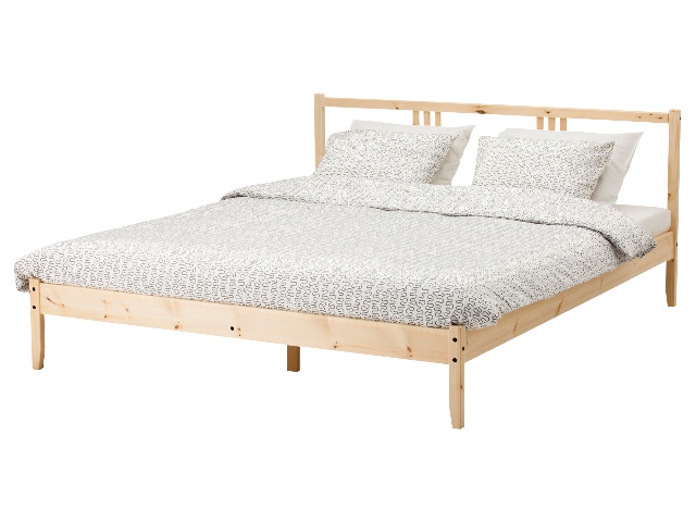
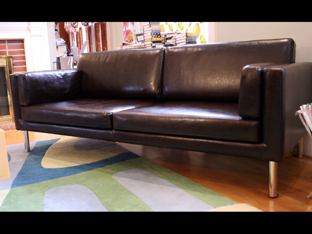
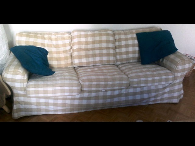
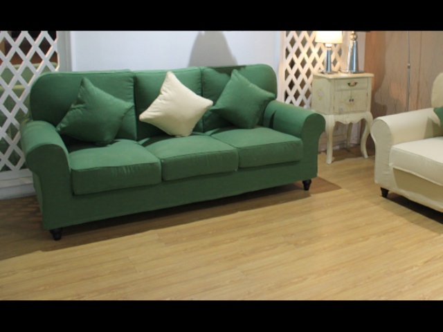
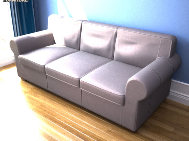
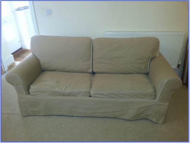
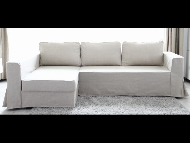
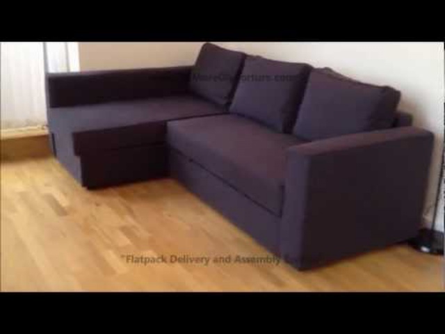
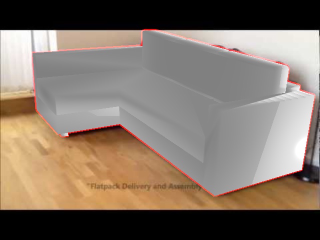
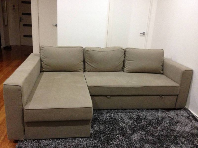
In this section, we provide more qualitative results of our approach. Figures 11–18 show additional results for the chair, bed, sofa, and table classes in the Pix3D dataset. Figures 19 and 20 show additional results for the Stanford cars and CompCars datasets, respectively. The qualitative results demonstrate the high accuracy of the alignments obtained by our approach despite variation in focal length, variability of the 3D models that have often very little texture, occlusions, and cluttered backgrounds. Finally, Figure 21 shows additional examples of failure modes on the Pix3D dataset.
For Pix3D, we provide good results for the chair class in Fig. 11 and Fig. 12, for the bed class in Fig. 13 and Fig. 14, for the sofa class in Fig. 15 and Fig. 16 and for the table class in Fig. 17 and Fig. 18. We also provide qualitative results for Stanford cars in Fig. 19 and for CompCars in Fig. 20. Please notice the quality of alignment that our approach can achieve. We provide the failure cases for the Pix3D dataset in Fig. 21.
Input image

Ground truth

Our prediction


Input image

Ground truth

Our prediction


Input image

Ground truth

Our prediction




Input image

Ground truth

Our prediction


Input image
Ground truth

Our prediction









Input image

Ground truth

Our prediction







Input image

Ground truth

Our prediction


Input image

Ground truth

Our prediction


Input image

Ground truth

Our prediction


Input image

Ground truth

Our prediction


1
Input image
 Ground truth
 Our prediction

2


3


4


5


6


7


