Interplay between Pair Density Wave and a Nested Fermi Surface

Introduction. — A pair density wave (PDW) is a superconducting (SC) state in which Cooper pairs carry finite momentum and its SC order parameter is spatially modulated without external magnetic field Berg et al. 2007; Agterberg and Tsunetsugu 2008; Berg et al. 2009; Berg et al. 2010; Jaefari and Fradkin 2012; Cho et al. 2012; Soto-Garrido and Fradkin 2014; Lee 2014; Maciejko and Nandkishore 2014; Wang et al. 2015; Jian et al. 2015; Jian et al. 2017; Wang et al. 2018; Venderley and Kim 2019; Han et al. 2020; Slagle and Fu 2020; Zhou and Wang 2021; Huang et al. 2022; Wu et al. 2022 (see, e.g. a recent review Agterberg et al. 2020). Such kind of state is similar to the one proposed earlier by Fulde-Ferrell (FF) Fulde and Ferrell 1964 and Larkin-Ovchinnikov (LO) Larkin and Ovchinnikov 1969 (together known as FFLO) in magnetic field above the Pauli limit. As a mother state for various descendant orders, e.g., charge density wave (CDW), loop current, and charge-$4e$ superconductivity, PDW has been receiving increasing attentions from diverse fields in physics Agterberg et al. 2020; Casalbuoni and Nardulli 2004. In particular, PDW was recently proposed as a promising candidate for explaining various interesting phenomena in cuprates and other strongly correlated systems Agterberg et al. 2020; Hamidian et al. 2016; Ruan et al. 2018; Edkins et al. 2019; Li et al. 2021.

In previous studies of PDW, only electrons near hot spots on Fermi surface (FS) can come into being finite momentum Cooper pairs and are gapped, while other parts of FS remain gapless. In contrast, as will be revealed in this work, the FS nesting feature admits full PDW pairing around the FS, that will gain more condensation energy than the partial pairing usually, while in-gap quasi-particle excitations are still allowed. Thus, it would be of great interest to examine the interplay between these two, PDW and FS nesting. (Note that the role of FS nesting was considered mostly to CDW or spin-density-wave, e.g. see Ref. Peierls 1955; Fröhlich 1954; Grüner 1988; Overhauser 1960; Overhauser 1962; Grüner 1994).

In this letter, we study PDW ordering in the presence of a nested FS on hexagonal lattices. We found that a time reversal symmetry (TRS) breaking PDW state is energetically favored. Bogoliubov quasi-particle excitations, density of states (DOS), local DOS (LDOS), and electron spectral function will be investigated as well as the quasi-particle interference (QPI) in scanning tunnelling microscopy (STM). The implications to recently discovered Kagome SC AV₃Sb₅(A=K,Rb,Cs) will be discussed.

Model. — We start with a single band model on a hexagonal lattice, on which the FS is nested as illustrated in Fig. 1. The Hamiltonian takes the form:

where $c^{\dagger}_{\mathbf{k},\sigma}(c_{\mathbf{k},\sigma})$ is electron creation (annihilation) operator with momentum $\mathbf{k}$ and spin $\sigma=\uparrow,\downarrow$, $\xi_{\mathbf{k}}=\epsilon_{\mathbf{k}}-\mu$ is the energy measured from the chemical potential $\mu$. $\Delta_{\pm\mathbf{Q}_{\alpha}}(\mathbf{k})=\Delta_{\pm\mathbf{Q}_{\alpha}}\text{exp}\left[-(|\xi_{\mathbf{k}}|+|\xi_{-\mathbf{k}\pm\mathbf{Q}_{\alpha}}|)/(2\Lambda)\right]$ ($\alpha=1,2,3$) indicates the Cooper pairing with total momentum $\pm\mathbf{Q}_{\alpha}$. Here $\Lambda$ is an energy cutoff. Setting lattice constant $a=1$, we consider $\mathbf{Q}_{1},\mathbf{Q}_{2},\mathbf{Q}_{3}=\left(0,\frac{\pi}{\sqrt{3}}\right),\left(-\frac{\pi}{2},-\frac{\pi}{2\sqrt{3}}\right),\left(\frac{\pi}{2},-\frac{\pi}{2\sqrt{3}}\right)$, since they are most relevant to CsV₃Sb₅ for which experimental evidences of period 4 PDW was recently reported Chen et al. 2021. As shown in Fig. 1(a), a hexagonal and nested FS can be realized by choosing $\mu$ or the electron filling properly. As a simple example, we focus on a triangular lattice, set the nearest neighboring (NN) hopping integral $t=1$, and choose $\mu=2$ (or $3/4$ filling), such that $\xi_{\mathbf{k}}=-2\left[\cos\left(k_{x}\right)+\cos\left(\frac{1}{2}k_{x}+\frac{\sqrt{3}}{2}k_{y}\right)+\cos\left(\frac{1}{2}k_{x}-\frac{\sqrt{3}}{2}k_{y}\right)+1\right]$. Note that our main results will also be applicable to more generic situations, including honeycomb and Kagome lattices.

From Fig. 1(b), one sees that each $\mathbf{k}$ on a FS segment along the $\mathbf{Q}_{\alpha}$ direction has at least two counterparts $-\mathbf{k}\pm\mathbf{Q}_{\alpha}$ to form finite momentum Cooper pairs. Moreover, $M$ and $X$ points have four momenta for pairing. These mean that the nesting feature allows full pairing in the region near the FS, which is in contrast with generic FS without nesting.

Time reversal symmetry. — The TRS of the Hamiltonian is respected if and only if $\xi_{-\mathbf{k}}=\xi_{\mathbf{k}}$ and $\Delta_{{\mathbf{Q}_{\alpha}}}^{\ast}(\mathbf{k}+\mathbf{Q}_{\alpha})=\Delta_{-\mathbf{Q}_{\alpha}}(\mathbf{k})$. For the aforementioned form of $\Delta_{\pm\mathbf{Q}_{\alpha}}(\mathbf{k})$, sufficient and necessary conditions for TRS reduce to $\Delta_{{\mathbf{Q}_{\alpha}}}^{\ast}=\Delta_{{-\mathbf{Q}_{\alpha}}}$.

The finite momentum pairing leads to a spatially varying pairing function in real space, resulting in a PDW. To be simple, we set $\Delta_{{\pm\mathbf{Q}_{\alpha}}}=\Delta e^{i\theta_{\alpha}}e^{\pm i\frac{\phi_{\alpha}}{2}}$, where $\Delta$ is real and positive, $\theta_{\alpha}\in(-\pi,\pi]$ and $\phi_{\alpha}\in(-\pi,\pi]$. Thus the pairing function $\Delta(\mathbf{r})$ reads

Commensurate PDW and descendant CDW order. — When the PDW melts partially, i.e., the $U(1)$ gauge symmetry is restored but not the translational symmetry, a descendant CDW order will arise with wave vectors $\mathbf{q}=\pm\mathbf{Q}_{\alpha}\pm\mathbf{Q}_{\beta}\neq{}\mathbf{0}$. These wave vectors can be classified into three sets: (B) $\mathbf{q}=\pm\mathbf{Q}_{\alpha}$ associated with a $4\times 4$ CDW; (C) $\mathbf{q}=\pm 2\mathbf{Q}_{\alpha}$ associated with a $2\times 2$ CDW; (D) $\mathbf{q}=\pm(\mathbf{Q}_{\alpha}-\mathbf{Q}_{\beta})$ associated with a $\frac{4}{\sqrt{3}}\times\frac{4}{\sqrt{3}}$ CDW [see Fig. 3(c)]. Note that the FS is nested by $\mathbf{q}=\pm 2\mathbf{Q}_{\alpha}$ in C but not those in B or D. So that the descendant CDW order can be of $4\times{}4$ and $\frac{4}{\sqrt{3}}\times\frac{4}{\sqrt{3}}$, in addition to the $2\times{}2$ CDW originating from the FS nesting.

Quasi-particles. — To study quasi-particle excitations in such a PDW associated with a $4\times{}4$ folded BZ, we introduce

and rewrite Eq. (1) in a matrix form:

Here $\hat{\mathcal{H}}_{\mathbf{k}}$ is a $32\times 32$ matrix, $\hat{D}(\mathbf{k})=\text{diag}\{\xi_{\mathbf{k}_{i}}\}$, $\mathbf{k}_{i}$ is the $i$-th momentum in $\hat{C}^{\dagger}_{\mathbf{k},\uparrow}$, and $\hat{\Delta}(\mathbf{k})$ is a $16\times 16$ matrix defined by $\Delta_{\pm\mathbf{Q}_{\alpha}}(\mathbf{k})$.

The diagonalization of $\hat{\mathcal{H}}_{\mathbf{k}}$ leads to

where $E(\mathbf{k})^{+(-)}_{i}\left[i\,(17-i)=1,\cdots,16\right]$ are quasi-particles (holes) energy spectra arranged in ascending order. The particle-hole symmetry (PHS) is manifested by $E(\mathbf{k})^{+}_{i}=-E(-\mathbf{k})^{-}_{i}$, which would give rise to $E(\mathbf{k})^{+}_{i}=-E(\mathbf{k})^{-}_{i}$ if the TRS was respected. $\gamma_{\mathbf{k},\uparrow(\downarrow),i}$’s are Bogoliubov quasi-particle operators, and $C^{\dagger}_{\mathbf{k},\uparrow,i}$ can be written in terms of them,

where $u(\mathbf{k})_{ij}$ and $v(\mathbf{k})_{ij}$ form a unitary transformation. It is easy to verify that: $E(\mathbf{k})_{i}^{\pm}=E(\mathbf{k}\pm\mathbf{Q}_{\alpha})_{i}^{\pm}$ and $\gamma_{\mathbf{k},\sigma,i}=\gamma_{\mathbf{k}\pm\mathbf{Q}_{\alpha},\sigma,i}$, i.e., the BZ is of $4\times{}4$ folding.

$\mathbb{Z}_{2}$ symmetry. — It is found that there exists additional $\mathbb{Z}_{2}$ symmetries associated with a theorem as follows.

Theorem: For each $\alpha$, the transformation $\Delta_{\pm\mathbf{Q}_{\alpha}}\mapsto-\Delta_{\pm\mathbf{Q}_{\alpha}}$ does not change the energy spectra of the system.

The proof of the theorem can be found in the Supplementary Material app. This theorem suggests a $\mathbb{Z}_{2}\times\mathbb{Z}_{2}$ symmetry, since only two of $\mathbf{Q}_{\alpha}$ are independent.

Approximate $E(\mathbf{k})^{+}_{1}$. — To get insight into low energy excitations, we inspect the lowest branch of quasi-particle dispersion, $E(\mathbf{k})^{+}_{1}$, along the FS. Without loss of generality, we consider the FS segment $M-X$ [see Figs. 1(a) and 1(b)]. For each $\mathbf{k}$ on this segment and away from $M$ and $X$ points, it is found that only the pairings between $\mathbf{k}$ and $-\mathbf{k}\pm\mathbf{Q}_{1}$ are of order of $\Delta$, while other pairing terms are much smaller than them because of the energy cutoff. Keeping sizable terms in $\hat{\Delta}(\mathbf{k})$ and neglecting others, we find that $\hat{\mathcal{H}}_{\mathbf{k}}$ can be approximately decomposed into paired and unpaired parts, i.e., $\hat{\mathcal{H}}_{\mathbf{k}}\approx\hat{\mathcal{H}}_{\mathbf{k}}^{p}\oplus\hat{\mathcal{H}}_{\mathbf{k}}^{f}$ app. Therefore $E(\mathbf{k})^{+}_{1}$ can be estimated as

It takes the minimum $E^{p}(\mathbf{k})_{\text{min}}=0$ at $\phi_{1}=0,\pi$ and the maximum $E^{p}(\mathbf{k})_{\text{max}}=\sqrt{2}\Delta$ at $\phi_{1}=\pm\frac{\pi}{2}$. Thus, the condensation of Cooper pairs will gain most energy at $\phi_{\alpha}=\pm\frac{\pi}{2}$. Meanwhile, $E^{f}(\mathbf{k})$ determined by $\hat{\mathcal{H}}_{\mathbf{k}}^{f}$ is responsible for (nearly) unpaired electrons and in-gap excitations in $E(\mathbf{k})^{+}_{1}$ as long as $E^{f}(\mathbf{k})<E^{p}(\mathbf{k})$. The combination of $E^{p}(\mathbf{k})$ and $E^{f}(\mathbf{k})$ gives rise to $E(\mathbf{k})^{+}_{1}$ approximately.

Away from the FS or near $M$ or $X$ point, other pairing terms become considerable and the simple decomposition of $\hat{\mathcal{H}}_{\mathbf{k}}$ does not work any more. We shall diagonalize $\hat{\mathcal{H}}_{\mathbf{k}}$ numerically, and study the ground state and low energy excitations. Hereafter we set $\Lambda=0.1$ and $\Delta=0.02$, unless otherwise specified.

Condensation energy. — The condensation energy $E_{c}\equiv{}E_{n}-E_{s}$, that defined by the energy difference between a SC ground state and corresponding normal state Schrieffer 1999, has been found as $E_{c}=\frac{1}{N}\sum_{\mathbf{k}}\left(\frac{1}{16}\sum_{i=1}^{16}\sum_{s=\pm}\sum_{E(\mathbf{k})^{s}_{i}>0}E(\mathbf{k})^{s}_{i}-|\xi_{\mathbf{k}}|\right)$. The numerical calculation finds that $E_{c}[\theta_{1},\theta_{2},\theta_{3},\phi_{\alpha}]$ reaches local maxima at $\phi_{\alpha}=\pm\pi/2$. This agrees with the above analysis of approximate $E(\mathbf{k})^{+}_{1}$ [see Eq. (6)] well. Moreover, as shown in Fig. 2 (a), the PDW state acquires maximum $E_{c}$ at $\phi_{\alpha}=\pm\pi/2$ and $\theta_{2}-\theta_{1}=\theta_{3}-\theta_{2}\equiv\pm 2\pi/3\,(\mathrm{mod}\,\pi)$, breaking the TRS spontaneously. Owing to the $\mathbb{Z}_{2}$ symmetry theorem, ($\theta_{\alpha}\mapsto\theta_{\alpha}\pm\pi$), the period is $\pi$ instead of $2\pi$ here.

Ginzburg-Landau free energy.— The TRS breaking and the $\mathbb{Z}_{2}$ symmetry can be verified in Ginzburg-Landau (GL) theory. Up to quartic order in $\Delta_{\mathbf{Q}_{\alpha}}$, the GL free energy can be written as app,

where $\mathcal{F}^{(0)}$ is $\Delta_{\mathbf{Q}_{\alpha}}$-independent, $\mathcal{F}^{(2)}=g^{(2)}\sum_{\alpha=1}^{3}\left(\left|\Delta_{\mathbf{Q}_{\alpha}}\right|^{2}+\left|\Delta_{-\mathbf{Q}_{\alpha}}\right|^{2}\right)$ with $g^{(2)}<0$, and $\mathcal{F}^{(4)}=\mathcal{F}^{(4)}_{0}+\mathcal{F}^{(4)}_{\phi}+\mathcal{F}^{(4)}_{\theta}$. Here $\mathcal{F}^{(4)}_{0}$ depends on $|\Delta_{\mathbf{Q}_{\alpha}}|$ only. $\mathcal{F}^{(4)}_{\phi}$ and $\mathcal{F}^{(4)}_{\theta}$ read

respectively, where both $g^{(4)}_{\phi}$ and $g^{(4)}_{\theta}$ are found to be positive and $\Delta_{\mathbf{Q}_{\alpha}}$-independent app. Putting $\Delta_{{\pm\mathbf{Q}_{\alpha}}}=\Delta e^{i\theta_{\alpha}}e^{\pm i\frac{\phi_{\alpha}}{2}}$ into the above leads to $\mathcal{F}^{(4)}_{\phi}=2g^{(4)}_{\phi}\Delta^{4}\sum_{\alpha=1}^{3}\cos\left(2\phi_{\alpha}\right)$ and $\mathcal{F}^{(4)}_{\theta}=2g^{(4)}_{\theta}\Delta^{4}\left[\cos\left(2\theta_{2}-2\theta_{1}\right)+\cos\left(2\theta_{3}-2\theta_{2}\right)+\cos\left(2\theta_{1}-2\theta_{3}\right)\right]$. Thus, the lowest free energy is achieved at $\phi_{\alpha}=\pm\pi/2$ and $\theta_{2}-\theta_{1}=\theta_{3}-\theta_{2}\equiv\pm 2\pi/3\,(\mathrm{mod}\,\pi)$.

Henceforward, we shall focus on the lowest energy state with $\theta_{1}=0$, $\theta_{2}=2\pi/3$, $\theta_{3}=-2\pi/3$ and $\phi_{\alpha}=\pi/2$, and study various electronic spectra.

Bogoliubov Fermi pockets. — As shown in Fig. 2 (b), around $M$ and $X$ points, $E(\mathbf{k})^{+}_{1}$ sinks down while $E(\mathbf{k})^{-}_{1}$ rises up, such that both of them go across zero energy. This means that quasi-particles (holes) possess FS indeed, namely, Bogoliubov Fermi pockets come into being. These Fermi pockets are located at $M$ and $X$ points and their periodic replica by the PDW (shifted by $\mathbf{q}=\pm\mathbf{Q}_{\alpha}\pm\mathbf{Q}_{\beta}\neq{}\mathbf{0}$), as indicated in Fig. 2 (c). It is displayed in Fig. 2 (d) that these Fermi pockets exhibit $D_{3}$ symmetry.

Density of States. — The differential conductance $dI/dV$ measured by STM Binnig and Rohrer 1987 is proportional to the DOS that reads $\rho(\omega)=-\frac{1}{8N}\sum_{\mathbf{k}}\sum_{i,j=1}^{16}\Big[|u(\mathbf{k})_{ij}|^{2}\frac{\partial n_{F}\left(\omega-E(\mathbf{k})_{j}^{+}\right)}{\partial\omega}+|v(\mathbf{k})_{ij}|^{2}\frac{\partial n_{F}\left(\omega-E(\mathbf{k})_{j}^{-}\right)}{\partial\omega}\Big]$, where $n_{F}$ is the Fermi distribution, and $u(\mathbf{k})_{ij}$ and $v(\mathbf{k})_{ij}$ are found via Eq. (5). As demonstrated in Fig. 3, for $k_{B}{}T=\Delta/60\ll\Delta$, $\rho(\omega)$ exhibits a mini-gap inside the SC gap manifested by sharp coherence peaks; while for $k_{B}{}T=\Delta/10\lesssim\Delta$, $\rho(\omega)$ (thereby $dI/dV$) curve is of V-shape. Note that both the mini-gap and the V-shape DOS suggest electronic excitations inside the SC gap. The extra peaks outside sharp coherence peaks are attributed to the Van Hove singularity Van Hove 1953, and the asymmetry between $\rho(\omega)$ and $\rho(-\omega)$ is due to the broken particle-hole symmetry in $\xi_{\mathbf{k}}$.

Local density of states. — Now we study the LDOS that serves as a standard tool to identify CDW orders by STM. The Fourier transformation of LDOS for the PDW state is given by $\rho(\mathbf{q},\omega)=-\frac{1}{8N}\sum_{\mathbf{k}}\sum_{i,j=1}^{16}\Big[u(\mathbf{k})_{ij}u^{*}(\mathbf{k}+\mathbf{q})_{ij}\frac{\partial n_{F}\left(\omega-E(\mathbf{k})_{j}^{+}\right)}{\partial\omega}+v(\mathbf{k})_{ij}v^{*}(\mathbf{k}+\mathbf{q})_{ij}\frac{\partial n_{F}\left(\omega-E(\mathbf{k})_{j}^{-}\right)}{\partial\omega}\Big]\bar{\delta}_{\mathbf{k},\mathbf{k}+\mathbf{q}}$, where $\bar{\delta}_{\mathbf{k},\mathbf{k}^{\prime}}\equiv\sum_{n,m=-\infty}^{\infty}\delta_{\mathbf{k}+n\mathbf{Q}_{1}+m\mathbf{Q}_{2},\mathbf{k}^{\prime}}$ app. It has been found that $\rho(\mathbf{q},\omega)$ does not vanish only at finite number of $\mathbf{q}$-points in BZ, as labeled in Fig. 3(c). These $\mathbf{q}$-points are nothing but wave vectors of the descendant CDW order. Note that $|\rho(\mathbf{q},\omega)|$ takes the same value at $\mathbf{q}$-points within each set of B, C or D app. As demonstrated in Fig. 3(d), $|\rho(\mathbf{q},\omega)|$ displays both (B) $4\times 4$ and (D) $4/\sqrt{3}\times 4/\sqrt{3}$ CDW orders in addition to (C) $2\times 2$ CDW order caused by the FS nesting. Define the integrated intensity of these CDW orders as $I_{CDW}(\mathbf{q})=\left|\int{}\rho(\mathbf{q},\omega)d\omega\right|/\left|\int\rho(\mathbf{q}=\mathbf{0},\omega)d\omega\right|$, we find that $I_{CDW}^{B,C,D}=1.51\times 10^{-5},1.02\times 10^{-5},2.82\times 10^{-6}$ at $k_{B}{}T=\Delta/10$ for the three types of CDW orders respectively.

Quasi-particle interference. — In the presence of elastic scatterings, the LDOS will be modulated due to the effect of QPI. To characterize this feature, we follow Ref. Wang and Lee 2003 to study the modulated LDOS $\delta\rho(\mathbf{r},\omega)$, or its Fourier transformation that is given by

where $\rho_{s}$ ($\rho$) is the LDOS in the presence (absence) of scatterings. $\widetilde{\text{Tr}}$ means tracing the upper-left $16\times 16$ block in a $32\times{}32$ matrix. $\hat{\mathcal{G}}(\mathbf{k},\omega+i\delta)=\left[(\omega+i\delta)\mathcal{I}-\hat{\mathcal{H}}_{\mathbf{k}}\right]^{-1}$ is Green’s function in the absence of scatterings and $\hat{T}(\omega)=\left[(V_{s}\hat{\tau}_{3})^{-1}-\frac{1}{N}\sum_{\mathbf{k}}\hat{\mathcal{G}}(\mathbf{k},\omega+i\delta)\right]^{-1}$ is the scattering matrix. Here $V_{s}$ is the nonmagnetic scattering impurity strength, and $\hat{\tau}_{3}$ is the Pauli matrix spanning Nambu space.

The modulation $|\delta\rho(\mathbf{q},\omega)|$ with $V_{s}=0.1$ at $\omega=0.01(<\Delta=0.02)$ is plotted in Fig. 4(a). For comparison, we also study QPI of a uniform s-wave superconductor, as shown in Fig. 4(b). In both figures the intensity at $\mathbf{q}=\mathbf{0}$ has been subtracted.

Electron spectral function. — The LDOS modulation due to scatterings can be analyzed by electron spectral function $A(\mathbf{k},\omega)=-\frac{1}{\pi}\text{Im}[\hat{\mathcal{G}}(\mathbf{k},\omega+i\delta)]_{11}$ in the absence of scattering. As is pointed out in Ref. Wang and Lee 2003, the summation in Eq. (9) is dominated by terms in which both $\mathbf{k}$ and $\mathbf{k}+\mathbf{q}$ are poles of $\hat{\mathcal{G}}$. Thus the vectors $\mathbf{q}$ associated with the scattering processes connecting two points with large $A(\mathbf{k},\omega)$ will show significant $|\delta\rho(\mathbf{q},\omega)|$. This feature of $\mathbf{q}$ is displayed in Fig. 4(c). An essential difference between the PDW state and a uniform s-wave state is that in-gap state is absent in the latter and the corresponding $A(\mathbf{k},\omega)$ and $|\delta\rho(\mathbf{q},\omega)|$ vanish at $\omega<\Delta$, as shown in Fig. 4(b) and (d). This also provides an experiment scheme to probe PDW states.

Discussions and conclusions. —

(i) Recently discovered Kagome SC AV₃Sb₅ (A=K,Rb,Cs) with a nearly $3/4$ filled electron band is a natural platform towards the realization of the interplay between PDW and FS nesting Ortiz et al. 2020; Ortiz et al. 2021a; Yin et al. 2021; Jiang et al. 2021a; Ortiz et al. 2021b; Kaboudvand et al. 2022. TRS breaking signatures have been extensively discussed both experimentally and theoretically in AV₃Sb₅ Jiang et al. 2021b; Yu et al. 2021; au2 et al. 2021; Feng et al. 2021; Lin and Nandkishore 2021a; Park et al. 2021. For the SC properties, the AV₃Sb₅ is shown to be a spin-singlet SC hosting s-wave features Mu et al. 2021; Duan et al. 2021; Xu et al. 2021. However, a residual thermal transport at $T=0$ and “multi-gap” V-shape DOS with residual zero-energy contributions were observed in SC states Zhao et al. 2021; Xu et al. 2021; Chen et al. 2021; Liang et al. 2021, which conflicts with the conventional s-wave nature. This contradiction can be resolved within the TRS breaking PDW scenario proposed in the present work. More importantly, a PDW state ordering at $\mathbf{Q}_{\alpha}$ has been observed in recent STM measurements Chen et al. 2021. Therefore, our theory may provide new insight into the PDW states and TRS breaking in AV₃Sb₅. Indeed, both $2\times 2$ and $4\times 4$ CDW have been observed in STM. Our theory suggests that the $\frac{4}{\sqrt{3}}\times\frac{4}{\sqrt{3}}$ CDW should appear as well, as long as the frequency $\omega$ is chosen properly.

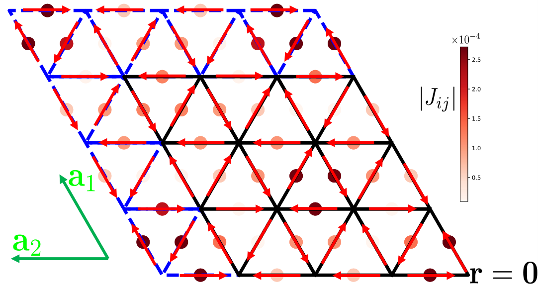
(ii) Indeed, such a TRS breaking SC state breaks the spatial inversion symmetry as well [see Eq. (2)], resulting in a chiral state with stable residual gapless quasi-particle excitations. The ground state is a flux state with spontaneous loop current Rodriguez and Douc¸ot 1992; Agterberg et al. 2015, as calculated in the Supplementary Material app. And the Bogoliubov Fermi pockets yield the linear $T$-dependent specific heat at low temperature.

(iii) One of remaining issues is what microscopic theory may give rise to the finite-momentum Cooper pairing instability on a nested FS. In the weak interaction limit, pairing at zero momentum is usually favored. Nonetheless, strong correlation might favor PDW instability against uniform pairing (see, e.g. Ref. Han et al. 2020; Zegrodnik and Spałek 2018). By establishing the microscopic model, the comparison with relevant models Honerkamp 2003; Wang et al. 2013; Nandkishore et al. 2014; Lin and Nandkishore 2021b based on the conventional CDW instabilities with nesting vector $2\mathbf{Q}_{\alpha}$ is one of the essential topics.

In summary, we have found that the FS nesting allows a full PDW pairing and in-gap states simultaneously. Such a PDW ansatz will give rise to a TRS breaking ground state. Subsequently, descendant CDW orders and various electronic spectra have been studied, and the relevance to newly discovered Kagome SC has been revealed.

Acknowledgment.— We thank Hui Chen, Shiyan Li, Zheng Li, Tao Wu, Fu-Chun Zhang, and Tong Zhang for helpful discussions. This work is partially supported by National Natural Science Foundation of China (No. 12274441, No. 12034004, No. 12174428 and No. 11825404), the K. C. Wong Education Foundation (Grant No. GJTD-2020-01), and the Strategic Priority Research Program of Chinese Academy of Sciences (No. XDB28000000).

Supplementary Material for "Interplay between Pair Density Wave and a Nested Fermi Surface"

This supplementary Material provides more details on our hexagonal lattice model, including the proof of $\mathbb{Z}_{2}$ symmetry theorem, the calculation of $E(\mathbf{k})^{+}_{1}$ along the FS segment, more numerical study on the condensation energy, ground state degeneracy and the derivation of Ginzburg-Landau free energy and local density of states.

References

• Berg et al. (2007) E. Berg, E. Fradkin, E.-A. Kim, S. A. Kivelson, V. Oganesyan, J. M. Tranquada, and S. C. Zhang, Dynamical layer decoupling in a stripe-ordered high-Tc{T}_{c} superconductor, Phys. Rev. Lett. 99, 127003 (2007).
• Agterberg and Tsunetsugu (2008) D. Agterberg and H. Tsunetsugu, Dislocations and vortices in pair-density-wave superconductors, Nature Physics 4, 639 (2008).
• Berg et al. (2009) E. Berg, E. Fradkin, S. A. Kivelson, and J. M. Tranquada, Striped superconductors: how spin, charge and superconducting orders intertwine in the cuprates, New Journal of Physics 11, 115004 (2009).
• Berg et al. (2010) E. Berg, E. Fradkin, and S. A. Kivelson, Pair-density-wave correlations in the kondo-heisenberg model, Phys. Rev. Lett. 105, 146403 (2010).
• Jaefari and Fradkin (2012) A. Jaefari and E. Fradkin, Pair-density-wave superconducting order in two-leg ladders, Phys. Rev. B 85, 035104 (2012).
• Cho et al. (2012) G. Y. Cho, J. H. Bardarson, Y.-M. Lu, and J. E. Moore, Superconductivity of doped weyl semimetals: Finite-momentum pairing and electronic analog of the 3 he-a phase, Phys. Rev. B 86, 214514 (2012).
• Soto-Garrido and Fradkin (2014) R. Soto-Garrido and E. Fradkin, Pair-density-wave superconducting states and electronic liquid-crystal phases, Phys. Rev. B 89, 165126 (2014).
• Lee (2014) P. A. Lee, Amperean pairing and the pseudogap phase of cuprate superconductors, Phys. Rev. X 4, 031017 (2014).
• Maciejko and Nandkishore (2014) J. Maciejko and R. Nandkishore, Weyl semimetals with short-range interactions, Phys. Rev. B 90, 035126 (2014).
• Wang et al. (2015) Y. Wang, D. F. Agterberg, and A. Chubukov, Coexistence of charge-density-wave and pair-density-wave orders in underdoped cuprates, Phys. Rev. Lett. 114, 197001 (2015).
• Jian et al. (2015) S.-K. Jian, Y.-F. Jiang, and H. Yao, Emergent spacetime supersymmetry in 3d weyl semimetals and 2d dirac semimetals, Phys. Rev. Lett. 114, 237001 (2015).
• Jian et al. (2017) S.-K. Jian, C.-H. Lin, J. Maciejko, and H. Yao, Emergence of supersymmetric quantum electrodynamics, Phys. Rev. Lett. 118, 166802 (2017).
• Wang et al. (2018) Y. Wang, S. D. Edkins, M. H. Hamidian, J. C. S. Davis, E. Fradkin, and S. A. Kivelson, Pair density waves in superconducting vortex halos, Phys. Rev. B 97, 174510 (2018).
• Venderley and Kim (2019) J. Venderley and E.-A. Kim, Evidence of pair-density wave in spin-valley locked systems, Science advances 5, eaat4698 (2019).
• Han et al. (2020) Z. Han, S. A. Kivelson, and H. Yao, Strong coupling limit of the holstein-hubbard model, Phys. Rev. Lett. 125, 167001 (2020).
• Slagle and Fu (2020) K. Slagle and L. Fu, Charge transfer excitations, pair density waves, and superconductivity in moiré materials, Phys. Rev. B 102, 235423 (2020).
• Zhou and Wang (2021) S. Zhou and Z. Wang, Chern fermi-pockets and chiral topological pair density waves in kagome superconductors, (2021), arXiv:2110.06266 [cond-mat.supr-con] .
• Huang et al. (2022) K. S. Huang, Z. Han, S. A. Kivelson, and H. Yao, Pair-density-wave in the strong coupling limit of the holstein-hubbard model, npj Quantum Materials 7, 17 (2022).
• Wu et al. (2022) Y.-M. Wu, Z. Wu, and H. Yao, Pair-density-wave and chiral superconductivity in twisted bilayer transition-metal-dichalcogenides, arXiv:2203.05480 (2022).
• Agterberg et al. (2020) D. F. Agterberg, J. S. Davis, S. D. Edkins, E. Fradkin, D. J. Van Harlingen, S. A. Kivelson, P. A. Lee, L. Radzihovsky, J. M. Tranquada, and Y. Wang, The physics of pair-density waves: Cuprate superconductors and beyond, Annual Review of Condensed Matter Physics 11, 231 (2020).
• Fulde and Ferrell (1964) P. Fulde and R. A. Ferrell, Superconductivity in a strong spin-exchange field, Phys. Rev. 135, A550 (1964).
• Larkin and Ovchinnikov (1969) A. I. Larkin and Y. N. Ovchinnikov, Quasiclassical Method in the Theory of Superconductivity, Sov. Phys. JETP 28, 1200 (1969).
• Casalbuoni and Nardulli (2004) R. Casalbuoni and G. Nardulli, Inhomogeneous superconductivity in condensed matter and QCD, Rev. Mod. Phys. 76, 263 (2004).
• Hamidian et al. (2016) M. H. Hamidian, S. D. Edkins, S. H. Joo, A. Kostin, H. Eisaki, S. Uchida, M. J. Lawler, E.-A. Kim, A. P. Mackenzie, K. Fujita, J. Lee, and J. C. S. Davis, Detection of a Cooper-pair density wave in Bi2Sr2CaCu2O8+x, Nature 532, 343 (2016).
• Ruan et al. (2018) W. Ruan, X. Li, C. Hu, Z. Hao, H. Li, P. Cai, X. Zhou, D.-H. Lee, and Y. Wang, Visualization of the periodic modulation of Cooper pairing in a cuprate superconductor, Nature Physics 14, 1178 (2018).
• Edkins et al. (2019) S. D. Edkins, A. Kostin, K. Fujita, A. P. Mackenzie, H. Eisaki, S. Uchida, S. Sachdev, M. J. Lawler, E.-A. Kim, J. C. S. Davis, and M. H. Hamidian, Magnetic field-induced pair density wave state in the cuprate vortex halo, Science 364, 976 (2019), https://www.science.org/doi/pdf/10.1126/science.aat1773 .
• Li et al. (2021) X. Li, C. Zou, Y. Ding, H. Yan, S. Ye, H. Li, Z. Hao, L. Zhao, X. Zhou, and Y. Wang, Evolution of charge and pair density modulations in overdoped Bi2​Sr2​CuO6+δ{\mathrm{Bi}}_{2}{\mathrm{Sr}}_{2}{\mathrm{CuO}}_{6+\delta}, Phys. Rev. X 11, 011007 (2021).
• Peierls (1955) R. E. Peierls, Quantum Theory of Solids ((Oxford University, New York/London), 1955).
• Fröhlich (1954) H. Fröhlich, On the theory of superconductivity: the one-dimensional case, Proceedings of the Royal Society of London. Series A. Mathematical and Physical Sciences 223, 296 (1954).
• Grüner (1988) G. Grüner, The dynamics of charge-density waves, Rev. Mod. Phys. 60, 1129 (1988).
• Overhauser (1960) A. W. Overhauser, Giant spin density waves, Phys. Rev. Lett. 4, 462 (1960).
• Overhauser (1962) A. W. Overhauser, Spin density waves in an electron gas, Phys. Rev. 128, 1437 (1962).
• Grüner (1994) G. Grüner, The dynamics of spin-density waves, Rev. Mod. Phys. 66, 1 (1994).
• Chen et al. (2021) H. Chen, H. Yang, B. Hu, Z. Zhao, J. Yuan, Y. Xing, G. Qian, Z. Huang, G. Li, Y. Ye, S. Ma, S. Ni, H. Zhang, Q. Yin, C. Gong, Z. Tu, H. Lei, H. Tan, S. Zhou, C. Shen, X. Dong, B. Yan, Z. Wang, and H.-J. Gao, Roton pair density wave in a strong-coupling kagome superconductor, Nature 599, 222 (2021).
• (35) Supplemental material, See the Supplemental Material for more details .
• Schrieffer (1999) J. R. Schrieffer, Theory of Superconductivity (Westview Press, 1999).
• Binnig and Rohrer (1987) G. Binnig and H. Rohrer, Scanning tunneling microscopy—from birth to adolescence, Rev. Mod. Phys. 59, 615 (1987).
• Van Hove (1953) L. Van Hove, The occurrence of singularities in the elastic frequency distribution of a crystal, Phys. Rev. 89, 1189 (1953).
• Wang and Lee (2003) Q.-H. Wang and D.-H. Lee, Quasiparticle scattering interference in high-temperature superconductors, Phys. Rev. B 67, 020511 (2003).
• Ortiz et al. (2020) B. R. Ortiz, S. M. L. Teicher, Y. Hu, J. L. Zuo, P. M. Sarte, E. C. Schueller, A. M. M. Abeykoon, M. J. Krogstad, S. Rosenkranz, R. Osborn, R. Seshadri, L. Balents, J. He, and S. D. Wilson, Csv3​sb5\mathrm{Cs}{\mathrm{v}}_{3}{\mathrm{sb}}_{5}: A 𝕫2{\mathbb{z}}_{2} topological kagome metal with a superconducting ground state, Phys. Rev. Lett. 125, 247002 (2020).
• Ortiz et al. (2021a) B. R. Ortiz, P. M. Sarte, E. M. Kenney, M. J. Graf, S. M. L. Teicher, R. Seshadri, and S. D. Wilson, Superconductivity in the 𝕫2{\mathbb{z}}_{2} kagome metal kv3​sb5{\mathrm{kv}}_{3}{\mathrm{sb}}_{5}, Phys. Rev. Materials 5, 034801 (2021a).
• Yin et al. (2021) Q. Yin, Z. Tu, C. Gong, Y. Fu, S. Yan, and H. Lei, Superconductivity and normal-state properties of kagome metal rbv3sb5 single crystals, Chinese Physics Letters 38, 037403 (2021).
• Jiang et al. (2021a) K. Jiang, T. Wu, J.-X. Yin, Z. Wang, M. Z. Hasan, S. D. Wilson, X. Chen, and J. Hu, Kagome superconductors av3sb5 (a=k, rb, cs), (2021a), arXiv:2109.10809 [cond-mat.supr-con] .
• Ortiz et al. (2021b) B. R. Ortiz, S. M. L. Teicher, L. Kautzsch, P. M. Sarte, N. Ratcliff, J. Harter, J. P. C. Ruff, R. Seshadri, and S. D. Wilson, Fermi surface mapping and the nature of charge-density-wave order in the kagome superconductor csv3​sb5{\mathrm{csv}}_{3}{\mathrm{sb}}_{5}, Phys. Rev. X 11, 041030 (2021b).
• Kaboudvand et al. (2022) F. Kaboudvand, S. M. L. Teicher, S. D. Wilson, R. Seshadri, and M. D. Johannes, Fermi surface nesting and the lindhard response function in the kagome superconductor csv3sb5, Applied Physics Letters 120, 111901 (2022).
• Jiang et al. (2021b) Y.-X. Jiang, J.-X. Yin, M. M. Denner, N. Shumiya, B. R. Ortiz, G. Xu, Z. Guguchia, J. He, M. S. Hossain, X. Liu, and et al., Unconventional chiral charge order in kagome superconductor kv3sb5, Nature Materials 20, 1353 (2021b).
• Yu et al. (2021) L. Yu, C. Wang, Y. Zhang, M. Sander, S. Ni, Z. Lu, S. Ma, Z. Wang, Z. Zhao, H. Chen, K. Jiang, Y. Zhang, H. Yang, F. Zhou, X. Dong, S. L. Johnson, M. J. Graf, J. Hu, H.-J. Gao, and Z. Zhao, Evidence of a hidden flux phase in the topological kagome metal csv3sb5, (2021), arXiv:2107.10714 [cond-mat.supr-con] .
• au2 et al. (2021) C. M. I. au2, D. Das, J. X. Yin, H. Liu, R. Gupta, Y. X. Jiang, M. Medarde, X. Wu, H. C. Lei, J. J. Chang, P. Dai, Q. Si, H. Miao, R. Thomale, T. Neupert, Y. Shi, R. Khasanov, M. Z. Hasan, H. Luetkens, and Z. Guguchia, Time-reversal symmetry-breaking charge order in a kagome superconductor, (2021), arXiv:2106.13443 [cond-mat.mtrl-sci] .
• Feng et al. (2021) X. Feng, K. Jiang, Z. Wang, and J. Hu, Chiral flux phase in the kagome superconductor av3sb5, Science Bulletin 66, 1384 (2021).
• Lin and Nandkishore (2021a) Y.-P. Lin and R. M. Nandkishore, Complex charge density waves at van hove singularity on hexagonal lattices: Haldane-model phase diagram and potential realization in the kagome metals a​V3​sb5a{V}_{3}{\mathrm{sb}}_{5} (aa=k, rb, cs), Phys. Rev. B 104, 045122 (2021a).
• Park et al. (2021) T. Park, M. Ye, and L. Balents, Electronic instabilities of kagome metals: Saddle points and landau theory, Phys. Rev. B 104, 035142 (2021).
• Mu et al. (2021) C. Mu, Q. Yin, Z. Tu, C. Gong, H. Lei, Z. Li, and J. Luo, Chin. Phys. Lett. 38, 077402 (2021).
• Duan et al. (2021) W. Duan, Z. Nie, S. Luo, F. Yu, B. R. Ortiz, L. Yin, H. Su, F. Du, A. Wang, Y. Chen, X. Lu, J. Ying, S. D. Wilson, X. Chen, Y. Song, and H. Yuan, Nodeless superconductivity in the kagome metal csv3sb5, Science China Physics, Mechanics & Astronomy 64, 107462 (2021).
• Xu et al. (2021) H.-S. Xu, Y.-J. Yan, R. Yin, W. Xia, S. Fang, Z. Chen, Y. Li, W. Yang, Y. Guo, and D.-L. Feng, Multiband superconductivity with sign-preserving order parameter in kagome superconductor csv3​sb5{\mathrm{csv}}_{3}{\mathrm{sb}}_{5}, Phys. Rev. Lett. 127, 187004 (2021).
• Zhao et al. (2021) C. C. Zhao, L. S. Wang, W. Xia, Q. W. Yin, J. M. Ni, Y. Y. Huang, C. P. Tu, Z. C. Tao, Z. J. Tu, C. S. Gong, H. C. Lei, Y. F. Guo, X. F. Yang, and S. Y. Li, Nodal superconductivity and superconducting domes in the topological kagome metal csv3sb5, (2021), arXiv:2102.08356 [cond-mat.supr-con] .
• Liang et al. (2021) Z. Liang, X. Hou, F. Zhang, W. Ma, P. Wu, Z. Zhang, F. Yu, J.-J. Ying, K. Jiang, L. Shan, Z. Wang, and X.-H. Chen, Three-dimensional charge density wave and surface-dependent vortex-core states in a kagome superconductor csv3​sb5{\mathrm{csv}}_{3}{\mathrm{sb}}_{5}, Phys. Rev. X 11, 031026 (2021).
• Rodriguez and Douc¸ot (1992) J. P. Rodriguez and B. Douc¸ot, Superconductivity, faraday effect, and optical absorption in the commensurate flux phase of the t-j model, Phys. Rev. B 45, 971 (1992).
• Agterberg et al. (2015) D. F. Agterberg, D. S. Melchert, and M. K. Kashyap, Emergent loop current order from pair density wave superconductivity, Phys. Rev. B 91, 054502 (2015).
• Zegrodnik and Spałek (2018) M. Zegrodnik and J. Spałek, Incorporation of charge- and pair-density-wave states into the one-band model of dd-wave superconductivity, Phys. Rev. B 98, 155144 (2018).
• Honerkamp (2003) C. Honerkamp, Instabilities of interacting electrons on the triangular lattice, Phys. Rev. B 68, 104510 (2003).
• Wang et al. (2013) W.-S. Wang, Z.-Z. Li, Y.-Y. Xiang, and Q.-H. Wang, Competing electronic orders on kagome lattices at van hove filling, Phys. Rev. B 87, 115135 (2013).
• Nandkishore et al. (2014) R. Nandkishore, R. Thomale, and A. V. Chubukov, Superconductivity from weak repulsion in hexagonal lattice systems, Phys. Rev. B 89, 144501 (2014).
• Lin and Nandkishore (2021b) Y.-P. Lin and R. M. Nandkishore, Multi-dome superconductivity in charge density wave kagome metals, arXiv:2107.09050 (2021b).