External control of a genetic toggle switch via Reinforcement Learning
Abstract
We investigate the problem of using a learning-based strategy to stabilize a synthetic toggle switch via an external control approach. To overcome the data efficiency problem that would render the algorithm unfeasible for practical use in synthetic biology, we adopt a sim-to-real paradigm where the policy is learnt via training on a simplified model of the toggle switch and it is then subsequently exploited to control a more realistic model of the switch parameterized from in-vivo experiments. Our in-silico experiments confirm the viability of the approach suggesting its potential use for in-vivo control implementations.
I Introduction
The problem of devising controllers to tame the dynamics of synthetic biological systems is becoming a crucial part of Synthetic Biology [15, 5] giving rise to the emerging field of cybergenetics [20]. In the external control paradigm, some phenotype of cells hosted in some environment (typically a turbidostat or a microfluidic chamber) is controlled via an external control action provided to the cells via actuated syringes whose motion is decided by some control strategy implemented in a PC or microcontroller. Examples of such approaches include those presented in [22] (see [15] for a review of other results from the literature).
Typically, either PI or MPC control strategies have been used to solve this problem (see [11] for a comparison of different techniques) despite the fact that models of the system under control are typically uncertain and that the sensed data are noisy. Moreover, running experiments is often costly and time-consuming and this can make model identification challenging in practice [5]. An alternative approach to address these issues could be to leverage learning-based control methods to learn the policy by directly interacting with the system. A key advantage of these methods is that knowledge of a well calibrated mathematical model is not necessarily required. However, the learning process can be sample inefficient, requiring long times and enough experimental data to learn the policy that could hinder its use in biology [2, 1].
A promising solution to overcome these problems is the sim-to-real approach where the control policy is first learnt on simulated environments and subsequently exported on the real system [14]. However, when this is done, one needs to verify that the sim-to-real gap can be bridged; i.e., that the policy learnt on the simulated environment can also control the real system.
In this paper, we focus on the problem of stabilizing a synthetic toggle switch about its unstable equilibrium point.
Such a problem is a widely adopted benchmark, see e.g. [18], in control applications to synthetic biology, which has been proposed as the equivalent in synthetic biology of of the swinging-up problem of an inverted pendulum in classical control. It is also a problem of practical interest as this bistable system is a fundamental synthetic circuit to endow cells with memory-like features [13] or to differentiate mono-strain cultures in different populations [17, 21]
Here, we explore the use of tabular learning to solve the problem adopting an external control setting where the control input is delivered implementing in-silico a realistic experimental set-up with actuation and sensing constraints. To overcome the data efficiency problem that would render the algorithm unfeasible for practical use in synthetic biology, we adopt a sim-to-real paradigm where the policy is learnt via training on a simplified model of the toggle switch and it is then exploited to control a more realistic, higher-dimensional model of the switch parameterized from in-vivo experiments in [18]. We show via a set of exhaustive in-silico experiments that such approach can effectively bridge the sim-to-real gap and, therefore, that learning-based strategies can be used for the control of synthetic biological systems. To benchmark our results against other state-of-the art algorithms for the toggle switch stabilization, we define and use a set of appropriate control metrics that confirm the effectiveness and viability of the proposed approach.
Related work
the problem of stabilizing the unstable equilibrium of the toggle switch has been recently considered in [18] where the regulation problem is solved via model-based open loop control, which exhibits poor robustness with respect to parameter variations. We also recall here [7], where a mathematical model describing the dynamics of the toggle switch when this is subject to periodic stimuli is presented. Based on this model, in [11] a closed-loop proportional integral pulse width modulation controller (PI-PWM) and a MPC strategy are proposed. Although exhibiting good performance and robustness properties, the PI-PWM requires the offline calibration of the control gains via an exhaustive search, while the MPC requires adequate computing power from the experimental platform in order to cope, in real time, with the computationally demanding optimization. In addition, both these strategies heavily rely on model identification of the system dynamics, which is usually subject to uncertainties both in structure and parameters [3]. We also recall here the strategy in [24], where a pulse-shaping controller is proposed to switch the system between its stable states, and the control strategies presented in [4], where a piecewise linear switched control is designed to either stabilize a simplified toggle switch model onto its unstable equilibrium or to switch between the stable equilibria. Literature on learning-based control of the toggle switch is sparse when compared to the literature on model-based approaches. To the best of our knowledge, the first and only work in this direction was reported in [25], where fitted Q-learning is used to toggle the switch between its stable equilibria, and the later extension of the approach to track periodic references reported in [23].
II The control problem
The genetic toggle switch is a gene regulatory network first engineered in E.coli in the early 2000 [9]. It is constructed around two repressors, LacI and TetR, each inhibithing the other expression (Fig. 1). The double inhibition chain enables the creation of hysteresis, making this circuit a simple implementation of a binary memory element. From a dynamical system viewpoint, this genetic pathway is a bistable dynamical system, exhibiting at steady-state either of two stable phenotypes where one of the repressors is fully expressed and the other is scarcely present. The steady state phenotype exhibited can be modified by laboratory interventions that induce a transition between the two stable states. Specifically, by adding two chemical inducers that diffuse through the cell membrane, i.e. anhydrotetracycline (aTc) and isopropyl--D-thiogalactoside (IPTG), it is possible to sequestrate TetR and LacI, respectively, relieving their inhibition on the competing repressor and toggling the system state.
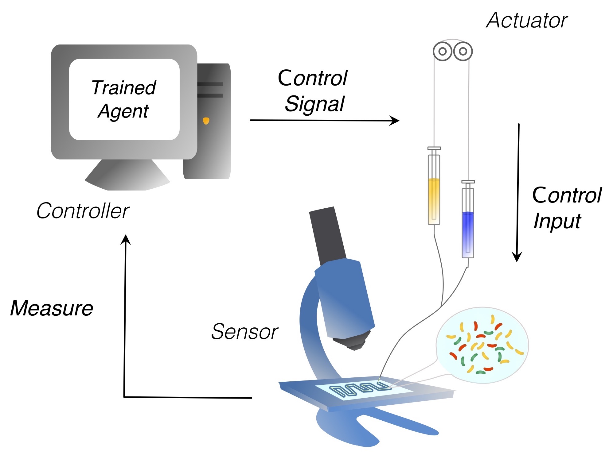
In this work we consider the problem of balancing the genetic toggle switch around its unstable equilibrium by modulating the concentration of the inducers in the growth environment. We address this problem by learning the policy via a model-free reinforcement learning algorithm. In our design, we explicitly account for biological and technological constraints of a real experimental set-up [8, 6], schematically shown in Fig. 2. As shown in the figure, the external control loop is implemented via a combination of microfluidics and inverted microscopy, through which it is possible to measure the fluorescence reporters expression level and to dynamically modify the composition of the growth medium. This experimental set-up, also described in [8, 6], introduces constraints on the time interval we can use to sample the state of the toggle switch and on the structure of the control input we can use to feed the cells. Namely, constraints are:
-
The state of each cell can be sampled up to once every 5 min, to avoid excessive phototossicity;
-
The concentration of the inducer molecules (i.e. the control inputs) can only be changed once every 15 min to limit osmotic stress on the cells;
-
The sum of the inputs needs to be a convex combination of the maximum levels of inducers used in the reservoirs. This is due to the specific implementation of the microfluidic device of choice.

III Mathematical Model
In what follows, we denote sets with calligraphic capital characters, vectors with bold letters and random variables with capital letters. We denote by and the set of real and non-negative real numbers, respectively. Letting , then denotes the diagonal matrix having on its main diagonal. All the quantities with the subscript refer to a discrete time domain.
III-A Deterministic modeling
We introduce the mathematical model for the toggle switch that we will use later on for the in-silico validations. Letting be the concentration of the mRNA associated with the lacI gene (), the concentration of the mRNA coding for TetR (), the concentration of LacI, and the concentration of TetR, using the pseudo reactions from [18], the dynamics of the system can be described via the following set of ODEs [7]:
| (1a) | ||||
| (1b) | ||||
| (1c) | ||||
| (1d) | ||||
where , , , , are basal transcription, maximal transcription, translation, mRNA degradation and protein degradation rates respectively, while and are two inputs. Physically, these are the intra-cellular concentrations of aTc and IPTG, respectively. Note that and cannot be directly manipulated as we can only modify the concentration of the inducers in the culture media, setting their extra-cellular concentrations, say and . Extra-cellular and intra-cellular inducer concentrations are linked together through the diffusion dynamics across the membrane. Specifically, as in [18], we complemented the model in (1) with further equations describing diffusion:
| (2a) | ||||
| (2b) | ||||
The functions and in (1) are Hill functions modeling the inhibition performed by LacI () and TetR (). These are defined as
| (3a) | ||||
| (3b) | ||||
where , , and are constant positive parameters describing the dissociation constants and the hill coefficients, respectively. In (3) there are two other Hill functions modeling the repression relief actuated by aTc () and IPTG ()
| (4a) | ||||
| (4b) | ||||
where parameters , , , have analogous meanings to those in (3).
III-B Stochastic model
In our in-silico validations, we also consider the stochastic version of (1) obtained from the Chemical Master Equation [10, 21, 18]. Specifically, following the arguments therein, we let be the stoichiometric matrix of the toggle switch given by
| (5) |
and be the propensity vector which, for the toggle switch, is given by
| (6) |
Then, the stochastic dynamics of the toggle switch can be given as
| (7) |
where and are independent standard Wiener process increments [16].
| mRNA | |||
|---|---|---|---|
| mRNA | |||
| mRNA | |||
| mRNA | |||
| a.u. | |||
| a.u. | |||
IV Training approach
The intrinsic stochasticity of the biochemical reactions involved in the toggle switch makes model-based control approaches not always viable as they might lack robustness during in-vivo validation [18]. For this reason, we propose the use of a Q-learning algorithm (QL) in its classical tabular version to train an artificial agent using a standard -greedy policy [26]. Differently from [25], the goal here is to stabilize the switch onto its unstable equilibrium rather than toggling it from one stable equilibrium to the other.
IV-A Control training approach
To overcome the challenge of limited in-vivo experiments that can be carried out to train the controller, we carry out the training using synthetic data generated via a simplified model of the switch that can be obtained from (1) by using time scale separation, see [7] for its derivation.
In particular we adopt the simplified adimensional model from [7]:
| (8a) | ||||
| (8b) | ||||
where
| (9) |
with , , and being positive coefficients. The nonlinear function models the static relationship between the repressor protein LacI and its inducer molecule aTc, while models the static relationship between the repressor protein TetR and its inducer molecule IPTG. Formally, these are defined as
The values of all the parameters used in the in-silico experiments are reported in Table I.
IV-B Training Results
Assuming the diffusion of the inducer molecules through the cell membrane to be faster than the biochemical processes hosted in the cell, during training we neglected (2) by setting and . Such an assumption will be later removed when applying the learnt policy to the more realistic toggle switch model of interest. Hence, providing further testing of whether the sim-to-real gap can be effectively bridged. In our design, we fulfilled constraints and (see Sec. II) by allowing the learning algorithm to measure the state of the system and modify the control inputs only once every minutes. This corresponds to setting the sampling time of the virtual agent in the dimensionless model (9). Finally, we fulfilled constraint by enforcing the following conditions on and :
| (10) |
The QL was then used to learn the policy adjusting (rather than for and ). In the above expression , and are the maximum values allowed for for the inducers’ concentrations.
For the sake of comparison, we assumed as in [11] that the goal is to stabilize the system around the desired equilibrium point . In addition, we discretized the action-state space as follows. The action space was sampled in 11 equally spaced values, while the states were discretized non-uniformly in the region which was heuristically found to be large enough. Specifically, we discretized each state in the region with a step of , while using a discretization step of elsewhere. By doing so, the artificial agent has a finer precision around the regulation point , reducing the steady state error. As reward function, we selected the quadratic function
| (11) |
We trained the virtual agent by running trials of episodes each; an episode consisting of an in-silico control experiment lasting hours. We set the learning rate as , the probability of taking an exploratory move and the discount factor . Results of the training are depicted in in Fig. 3 where the evolution of the cumulative reward is expressed in terms of mean and standard deviation over the realizations of the training process starting from the same initial conditions . We notice that the learning process reaches convergence on average within the first 200 episodes. For the sake of brevity, we do not show here the performance of the learnt control policy on the simplified model it was trained upon but choose to show later (see Fig. 4) its performance on the more realistic models presented in Sec. III.
V In-silico validation on a realistic model
We validated the performance of the control policy learnt on synthetic data generated by the simplified model by applying it to control the more realistic, higher-dimensional, deterministic and a stochastic models presented in Sec. III which are used as proxies of a possible in-vivo implementation of the toggle switch (as also done in [18]).
V-A Metrics
We compared the performance of the control algorithm developed in this work with the PI-PWM and MPC strategies presented in [11]. Specifically, we quantified the effectiveness of each control strategy using the set of metrics introduced in [8, 11]. Namely, we computed the Integral Square Error (ISE), defined as
| (12) |
which measures the average transient and steady state performances. In addition, we evaluated the Integral Time-weighted Absolute Error (ITAE) defined as
| (13) |
which weighs the error more as the time progresses, making residual errors at steady state more relevant towards the computation of the control metric. In Equations (12)-(13) is computed as
| (14) |
with and being the moving averages of and over a window of width , formally defined as
Both metrics are evaluated from up to the control horizon .
V-B Deterministic experiments
Fig. 4.a shows the control performance of the learnt control strategy when applied to the realistic deterministic model (1) showing the effectiveness of the proposed training strategy. Table II shows a quantitative comparison between the strategy presented here with the MPC and PI-PWM previously described in [11], when both are tested on (1). We see that the performance achieved by the QL based controller are comparable with the model-based ones. In particular, the model free QL is capable of outperforming the PI-PWM in terms of ISE, reducing the variability of the proteins during the transient.
V-C Stochastic experiments
Next we test the robustness of the proposed approach by running a set of in-silico experiments using the stochastic model of the toggle switch presented in Sec. III-B using a Euler-Maurayama scheme with for its efficient numerical implementation [12]. The outcome of the in-silico experiments are reported in Fig. 4.b. Table II shows the quantitative comparison between QL, MPC and PI-PWM when applied to the stochastic model. Again, we see that the QL based controller shows comparable performance when contrasted with model-based ones for the control of the full model confirming the viability of a sim-to-real paradigm in a biological setting.
VI Conclusions
We investigated the problem of stabilizing the unstable equilibrium of a genetic toggle switch using via an external control approach based on machine learning. To overcome the data efficiency problem that would render the algorithm unfeasible for practical use in synthetic biology, we adopted and tested in-silico the use of a sim-to-real paradigm. That is, the policy was first learnt via training on a simplified model of the toggle switch and it was then subsequently exploited to control a more realistic model of the switch parameterized from in-vivo experiments.
Our in-silico experiments confirmed the viability of this approach suggesting its potential use for in-vivo control implementations. This represents a crucial step towards the deployment of learning algorithms to control synthetic biological circuits. Ongoing research is aimed at testing the proposed strategy in-vivo using the microfluidics platform described in [19].
| QL | QL | MPC | PI-PWM | |
|---|---|---|---|---|
| quasi-steady | complete | |||
| state assumption | model | |||
| Deterministic in-silico experiments | ||||
| ISE | ||||
| ITAE | ||||
| Stochastic in-silico experiments | ||||
| ISE | ||||
| ITAE | ||||
References
- [1] Dimitri. Bertsekas “Dynamic Programming and Optimal Control” Belmont, MA, USA: Athena Scientific, 2005
- [2] Lucian Buşoniu et al. “Reinforcement learning for control: Performance, stability, and deep approximators” In Annual Reviews in Control 46, 2018, pp. 8–28
- [3] Stefano Cardinale and Adam Arkin “Contextualizing context for synthetic biology–identifying causes of failure of synthetic biological systems” In Biotechnology journal 7.7, 2012, pp. 856–866
- [4] Lucie Chambon and Jean-Luc Gouzé “A new qualitative control strategy for the genetic Toggle Switch” In IFAC-PapersOnLine 52.1, 2019, pp. 532–537
- [5] Domitilla Del, Yili Qian, Richard Murray and Eduardo Sontag “Future systems and control research in synthetic biology” In Annual Reviews in Control 45 Elsevier, 2018, pp. 5–17
- [6] Mike Ferry, Ivan Razinkov and Jeff Hasty “Microfluidics for synthetic biology: from design to execution” In Methods in enzymology 497, 2011, pp. 295–372
- [7] Davide Fiore, Agostino Guarino and Mario Di “Analysis and control of genetic toggle switches subject to periodic multi-input stimulation” In IEEE control systems letters 3.2, 2018, pp. 278–283
- [8] Gianfranco Fiore, Giansimone Perrino, Mario Di and Diego Di “In vivo real-time control of gene expression: a comparative analysis of feedback control strategies in yeast” In ACS synthetic biology 5.2, 2016, pp. 154–162
- [9] Timothy Gardner, Charles Cantor and James Collins “Construction of a genetic toggle switch in Escherichia coli” In Nature 403.6767, 2000, pp. 339–342
- [10] Daniel Gillespie “A rigorous derivation of the chemical master equation” In Physica A: Statistical Mechanics and its Applications 188.1-3, 1992, pp. 404–425
- [11] Agostino Guarino, Davide Fiore, Davide Salzano and Mario di Bernardo “Balancing cell populations endowed with a synthetic toggle switch via adaptive pulsatile feedback control” In ACS synthetic biology 9.4, 2020, pp. 793–803
- [12] Desmond Higham “An algorithmic introduction to numerical simulation of stochastic differential equations” In SIAM review 43.3 SIAM, 2001, pp. 525–546
- [13] Patrick Hillenbrand, Georg Fritz and Ulrich Gerland “Biological Signal Processing with a Genetic Toggle Switch” In PLOS One 8(7), 2013, pp. e68345
- [14] Stephen James, Andrew Davison and Edward Johns “Transferring end-to-end visuomotor control from simulation to real world for a multi-stage task” In Conference on Robot Learning, 2017, pp. 334–343 PMLR
- [15] M. Khammash, M. Di and D. Di “Cybergenetics: Theory and Methods for Genetic Control System” In 2019 IEEE 58th Conference on Decision and Control (CDC), 2019, pp. 916–926
- [16] Eszter Lakatos “Stochastic analysis and control methods for molecular cell biology”, 2017
- [17] Michel Laurent and Nicolas Kellershohn “Multistability: a major means of differentiation and evolution in biological systems” In Trends in Biochemical Sciences 24(11), 1999, pp. 418–422
- [18] Jean-Baptiste Lugagne et al. “Balancing a genetic toggle switch by real-time feedback control and periodic forcing” In Nature communications 8.1, 2017, pp. 1–8
- [19] Filippo Menolascina et al. “In-vivo real-time control of protein expression from endogenous and synthetic gene networks” In PLoS computational biology 10.5, 2014, pp. e1003625
- [20] Iacopo Ruolo et al. “Control engineering meets synthetic biology: Foundations and applications” In Current Opinion in Systems Biology 28 Elsevier, 2021, pp. 100397
- [21] Davide Salzano, Davide Fiore and Mario di Bernardo “Ratiometric control for differentiation of cell populations endowed with synthetic toggle switches” In 2019 IEEE 58th Conference on Decision and Control (CDC), 2019, pp. 927–932 IEEE
- [22] Barbara Shannon et al. “In vivo feedback control of an antithetic molecular-titration motif in Escherichia coli using microfluidics” In ACS Synthetic Biology 9.10 ACS Publications, 2020, pp. 2617–2624
- [23] Aivar Sootla et al. “On periodic reference tracking using batch-mode reinforcement learning with application to gene regulatory network control” In 52nd IEEE conference on decision and control, 2013, pp. 4086–4091
- [24] Aivar Sootla, Diego Oyarzún, David Angeli and Guy-Bart Stan “Shaping pulses to control bistable systems: Analysis, computation and counterexamples” In Automatica 63, 2016, pp. 254–264
- [25] Aivar Sootla et al. “Toggling a genetic switch using reinforcement learning” In arXiv preprint arXiv:1303.3183, 2013
- [26] Christopher Watkins and Peter Dayan “Q-learning” In Machine learning 8.3, 1992, pp. 279–292