Statistical Perspective on Functional and Causal Neural Connectomics: The Time-Aware PC Algorithm
Abstract
The representation of the flow of information between neurons in the brain based on their activity is termed the causal functional connectome. Such representation incorporates the dynamic nature of neuronal activity and causal interactions between them. In contrast to connectome, the causal functional connectome is not directly observed and needs to be inferred from neural time series. A popular statistical framework for inferring causal connectivity from observations is the directed probabilistic graphical modeling. Its common formulation is not suitable for neural time series since was developed for variables with independent and identically distributed static samples. In this work, we propose to model and estimate the causal functional connectivity from neural time series using a novel approach that adapts directed probabilistic graphical modeling to the time series scenario. In particular, we develop the Time-Aware PC (TPC) algorithm for estimating the causal functional connectivity, which adapts the PC algorithm a state-of-the-art method for statistical causal inference. We show that the model outcome of TPC has the properties of reflecting causality of neural interactions such as being non-parametric, exhibits the directed Markov property in a time-series setting, and is predictive of the consequence of counterfactual interventions on the time series. We demonstrate the utility of the methodology to obtain the causal functional connectome for several datasets including simulations, benchmark datasets, and recent multi-array electro-physiological recordings from the mouse visual cortex.
1 Introduction
Functional Connectome (FC) refers to the network of interactions between units of the brain, such as individual neurons or brain regions, with respect to their activity over time [1]. The aim of finding the FC is to provide insight into how neurons interact to form brain function. FC can be represented by a graph whose nodes represent neurons and edges indicate a relationship between the activity of connected neurons. The edges can either represent undirected stochastic associations between activity of neurons or directed causal relationships between activity of neurons. While association between neural activity describes whether neuron and neuron are active in a correlated manner, the ultimate goal of functional connectomics is to answer causal queries, such as whether the activity in neuron causes neuron to be active , or is it the other way around ? Else, does a neuron intermediate the correlation between and [2, 3, 4]?
When the interactions are causal, the network is termed as causal functional connectome (CFC). The CFC maps how neural activity flows within neural circuits, and provides the possibility for inference of neural pathways essential for brain functioning and behavior, such as sensory-motor-behavioral pathways [5]. Several approaches aim to infer CFC, such as Granger Causality (GC), Dynamic Causal Modeling (DCM), and Directed Probabilistic Graphical Models (DPGM), each having their applicability and challenges, as surveyed in [6]. GC obtains the directed functional connectivity from observed neural activity in a way that tells whether a neuron’s past is predictive of another neuron’s future, however it is unclear whether the prediction implies causation. In contrast, DCM compares specific mechanistic biological models based on data evidence, in which, model parameters represent causal influences between hidden neural states [7]. On the other hand, DPGM is a generic procedure to obtain causal relationships between nodes of a network from observations, using the directed Markov property. DPGM is non-parametric in the sense of capturing arbitrary functional relationships among the nodes and is predictive of the consequence of counterfactual interventions to the network [8, 9]. Such properties make DPGM a popular approach for causal modeling in various disciplines such as genomics and econometrics [10, 11, 12, 13, 14, 15, 16, 17, 18, 19, 20, 21].
The utility of DPGM in obtaining CFC from neural data has been investigated in [6]. DPGM, applicable to i.i.d. observations, can model causal relations between whole time series of different neurons in sense of average over time or at a specific time. Thereby, standard DPGM does not explicitly model the inter-temporal causal relations between neural activity in the time series. For inference of the DPGM, the PC algorithm is one of the widely used causal inference algorithms that assumes independent and identically distributed (i.i.d.) sampling of the nodes of the network and absence of latent confounders [22, 23]. However, in neural time series scenario, causal relations are between neural activity at different times. Assuming independent sampling of nodes of the common DPGM is not suitable as the nodes correspond to a time series with temporal dependency. Moreover, DPGM typically generate a Directed Acyclic Graph (DAG), while neural activity is often comprised of feedback loops over time [24, 25, 26, 27]. Though adaptations aim to include cycles in the DPGM they have a more complicated output [28]. Addressing these limitations will improve the utility of DPGM for finding CFC in the neural time series scenario and is the focus of this work.
In this work, we develop a novel approach for modeling and estimating causal functional connectivity by adapting directed probabilistic graphical models to the time series scenario. We introduce the Time-Aware PC (TPC) algorithm. It uses the PC algorithm as a starting point and adapts it to the neural time series setup by following processes such as time-delay, bootstrapping and pruning. These ensure that the inferred CFC is robust and well suited to the setup. The proposed CFC graphical model incorporates feedback loops in functional connectivity and is non-parametric, yet we show that the CFC graphical model accurately represents the causal relationships in the unknown dynamical process of neural activity. Furthermore, the proposed CFC graphical model is predictive of the consequence of counterfactual interventions, such as the alteration in the CFC due to ablation or external control of certain neurons. We apply the proposed methodology on neural signals simulated from different paradigms and CFC motifs and demonstrate the utility of TPC in recovering the generating motifs. We also apply the TPC on public benchmark datasets and compare the performance in recovery of the ground truth CFC with other approaches. We further demonstrate the use of TPC to obtain the CFC among sampled neurons in mice brain from electrophysiological neural signals.
The following is a list of acronyms used in this paper: Functional Connectivity (FC), Causal Functional Connectivity (CFC), Granger Causality (GC), Dynamic Causal Model (DCM), Directed Probabilistic Graphical Model (DPGM), Directed Markov Property (DMP), Functional Magnetic Resonance Imaging (fMRI), Probabilistic Graphical Model (PGM), i.i.d. (Independent and Identically Distributed), Markov Property (MP), Directed Acyclic Graph (DAG), Peter Clark (PC), Greedy Equivalence Search (GES), Greedy Interventional Equivalence Search (GIES), Continuous Time Recurrent Neural Network (CTRNN), True Positive (TP), False Positive (FP), True Negative (TN), False Negative (FN), True Positive Rate (TPR), False Positive Rate (FPR).
2 Causal Functional Connectivity for Static Variables - Review
In this section, we provide a concise summary of DPGM for finding CFC for static variables, i.e. variables with i.i.d. samples, and extend in later sections to incorporate temporal dependence in time series. Let us consider a brain network with neurons labeled as and denote a random variable measuring the activity of neuron at time . Examples for such variables are instantaneous membrane potential, instantaneous firing rate, etc. Let denote a scalar-valued random variable corresponding to , e.g., the neural recording at time : , average of recordings over time , and for a set of neurons , denotes the random vector . Let denote a directed acyclic graph (DAG), i.e., a directed graph without directed cycles, over the neurons in and with directed edges . Nodes and are said to be adjacent if or . A path is a sequence of distinct nodes in which successive nodes are adjacent. For a path , if every edge of is of the form then is an ancestor of and is a descendant of . The set of non-descendants of , denoted , contains nodes that are not descendants of . The set of parents of is denoted as . We mark the set as the set that contains all nodes which are older ancestors of before its parents [8, 9]. We use the convention that and .
With these notations, we highlight the Directed Markov Property (DMP) and its functional equivalence for DPGM. The DMP connects probabilistic conditional independencies between nodes of a directed graph with relationships of causal influence by ensuring that the influence of each node’s ancestors beyond parents reaches to the node exclusively via its parents. Furthermore, the functional equivalence for DPGM shows that, the edges in a DPGM satisfying the DMP are consistent with causal functional interactions among the nodes.
Directed Markov Property (DMP)
is said to satisfy the Directed Markov Property with respect to the DAG if and only if,
| (1) |
The DMP translates the edges in the DAG into conditional independencies, such that each node and its older ancestors are conditionally independent given its parents . The DMP can be equivalently represented with functional relationships between parent and child instead of conditional independencies, which is described in the following theorem [29].
Functional Equivalence of DMP
If satisfies
| (2) |
where are independent random variables and are measurable functions for and is a DAG with vertices , then satisfies the Directed Markov Property with respect to . Conversely, if satisfies the Directed Markov Property with respect to a DAG , then there are independent random variables and measurable functions for which Eq. (2) holds. This shows that if satisfies the DMP with respect to the DAG , then admits a natural causal interpretation, due to its functional equivalence: parent nodes of in causally influence the child node [30].
PC algorithm
Let satisfy the DMP with respect to the DAG . The PC algorithm is a popular method to infer from observed data [22]. The PC algorithm uses a consistent statistical test, such as Fisher’s Z-transform when are Gaussian variables, and kernel and distance based tests for non-Gaussian variables [31, 32]. The algorithm first represents the observed variables by nodes of a graph and starts with an empty set of edges and puts an undirected edge between each pair of nodes if they are independent or conditionally independent given any other variable(s) determined by the statistical test. This results in the undirected skeleton graph, which is then converted into a DAG by directing the undirected edges using rules for orientation. The PC algorithm estimates several DAGs based on i.i.d. samples of , and outputs a single completed partially directed acyclic graph (CPDAG) defined as follows: has a directed edge from node if is present in all the DAGs . It has an undirected edge between and if either directions between them are present among the DAGs . It has no edge between and if no edge is present between them in any of the DAGs . The CPDAG is uniquely identifiable from observed data.
The PC algorithm assumes causal sufficiency of the input variables: A set of variables is causally sufficient for a population if and only if in the population every common cause of any two or more variables in is in , or has the same value for all units in the population. Another method, the FCI algorithm, is applicable when causal sufficiency does not hold [33]. However, while the PC algorithm can identify direct causes, FCI algorithm cannot distinguish between direct and indirect causes.
Let denote the probability distribution of . The PC algorithm also assumes faithfulness of the DAG to : if the DMP with respect to encompasses all the conditional independence relations due to , is said to be faithful to . Using a consistent statistical test for conditional independence, and assuming causal sufficiency and faithfulness, the PC algorithm estimate, , is consistent for ; that is, converges in probability to with increasing number of samples in data [34, 22].
3 Causal Functional Connectivity for Time Series
In this section, we propose a novel methodology for modeling and estimation of the CFC for time series. This methodology is generic and applicable to various time series including neural recordings. The CFC is represented by a graph with nodes as neurons, each corresponds to a time series of neural activity, and edges indicating causal connectivity. In the following, we show we can explicitly model causal relations within and between time series in a DPGM framework and use it to define the CFC.
3.1 Unrolled Graphical Modeling of Time Series
We aim to incorporate the causal influence of the activity of neuron at time upon the activity of neuron at time in our proposed model. To do that, we unroll the time series into nodes for neuron and time where the node corresponds to the variable . We use directed edges between the nodes to represent causal relations between . For example, the edge represents the causal influence of the activity of neuron at time , upon the activity of neuron at time , . Let be the set of nodes in the unrolled time series, be the set of directed edges between the nodes and be the Unrolled Graph for the time series (See Figure 1-middle). We assume that is a DAG in which there are no cycles in the edges in .
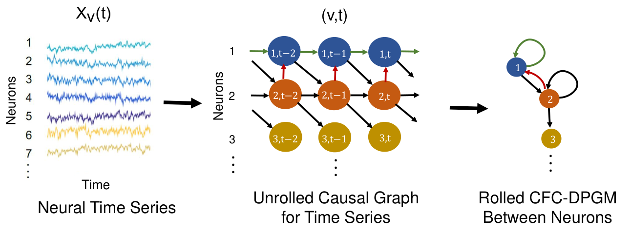
Causal relationships between neurons are either forward in time: (1) from neurons at time to neuron at time for , represented by for in ; or, (2) contemporaneous: when causal influences occur more rapidly than the sampling interval of the time series, represented in by at time [35, 36]. Causal relations cannot direct backward in time, that is, will not contain for . Furthermore, for the contemporaneous causal influences, we do not allow the activity of at time to have causal influence on itself at time , that is is not allowed, while is allowed. These considerations imply the absence of cycles in , thereby justifying the assumption for to be a DAG to model the causal interactions in the unrolled time series.
In practice, the true causal interactions between are unknown. Yet, when satisfies the DMP with respect to DAG , then it implies that captures the causal functional interactions among , as we show in the functional equivalence of DMP in Section 2. We refer to such a DAG as the Unrolled Causal Graph for the time series .
3.2 Rolled CFC-DPGM
Typically for signals, effective CFC representation refers to relations between neurons rather than relations between different signals’ times. Thereby, we propose to roll back the unrolled causal DAG to define CFC between neurons (See Figure 1-right). The rolled graph is based on the principle that the existence of a causal relationship from neuron at time to neuron at time , for , would imply that is connected to in the rolled CFC. In practice, the causal interactions weaken as the time-gap grows. Thereby, we consider a maximum time-delay of interaction, , so that and would not share a significant influence between them if the time gap for all neurons . Such a consideration of the maximum time-delay aids in making statistical inference from the time series data. Thus, if in for some , then the CFC graph between neurons should include . We consolidate these concepts to define causal functional connectivity between neurons based on DPGM, in the following.
Definition 1 (Rolled CFC-DPGM).
Let satisfy the DMP with respect to DAG . The Rolled CFC-DPGM for neurons in with maximum time-delay of interaction , is defined as the directed graph having edge if . , could be either the same neuron or distinct neurons.
We show an example in Figure 1, where for neurons , their unrolled DAG is represented by Figure 1-middle. When the neural data satisfies the directed Markov Property with respect to , the CFC graph with maximum time delay of interaction is given by Figure 1-right. Note that the same CFC graph would be obtained by taking any value of .
Property: The transformation from unrolled DAG to Rolled CFC, , is a well-defined function, meaning that starting from the same unrolled DAG we will not have multiple possible CFC and there will be a unique CFC .
Proof: By contradiction, consider two distinct CFCs and with obtained from the unrolled DAG . Since , so such that but , where could be either the same or distinct neurons. Using the definiton 1 of Rolled CFC-DPGM, implies that for some , . But contradicts this as it implies that for any .
Contemporaneous and Feedback Interactions
We highlight that the Rolled CFC-DPGM in Definition 1 incorporates contemporaneous interactions, which can arise if the causal influences occur more rapidly than the sampling interval of the time series or the aggregation interval for aggregated time series. Such a scenario can arise for example in spiking neural datasets where peri-stimulus time histograms aggregate the spike trains over time intervals [37, 38], and in Functional Magnetic Resonance Imaging (fMRI) datasets where low sampling rates is typical [39]. However, if the time span in sampling and aggregation is expected to be less than the time scale of causal interactions, then one can impose to exclude contemporaneous interactions. Additionally, the Rolled CFC-DPGM accomodates self-loops in neural interactions [40, 41], by checking whether for some in determining whether . Longer feedback loops are also incorporated. For example, the existence of is determined by checking whether and for some . By virtue of the technique of unrolling and rolling back, the Rolled CFC-DPGM captures causality while including cycles, since the Unrolled Graph is still a DAG and thereby meets the requirement for satisfying DMP.

3.3 Estimation from data: Time-Aware PC (TPC) Algorithm
In this section we outline the steps to estimate the Rolled CFC-DPGM from dataset , , which constitute the Time-Aware PC (TPC) Algorithm. The output of TPC is a Rolled CFC that contains edges found significant in the duration of recording. The TPC Algorithm first aims to estimate the unrolled DAG for , considering maximum time-delay of interaction . The unrolled DAG has nodes as and with respect to which satisfies the DMP. To perform the estimation, TPC constructs samples for a node consisting of time delayed instances of , denoted , with a time delay of , i.e. with a shift backward of the signal by . Such a time-delay of multiples of ensures a substantial time-gap of units between samples, that reduces interdependence between the samples, considering the maximum time-delay of interaction . This operation increases the number of considered time-series by a multiple of such that for original recordings of nodes in , there would be nodes in .
- Step 1.
Time-Delayed Samples. For , construct -th sample for , denoted , by time-delay of : , .
- Step 2.
Bootstrap. For , select a random window from to obtain , by drawing a random integer , and .
- Step 3.
PC. Use PC algorithm to estimate the unrolled DAG for over , , with the samples , for . Denote the output as .
- Step 4.
Orient. Reverse the edge directions of edges , when and update .
- Step 5.
- Step 6.
Robust edges.
- (a)
Repeat Steps 2-5 to obtain iterates of the rolled CFC-DPGM: , and connectivity weights , .
- (b)
Output a single CFC, , with only those edges whose relative frequency of occurrence among is above .
- (c)
Output single Connectivity Weights, , for connections , as the average of when the set is non-empty and otherwise.
- (a)
- Step 7.
Pruning. Remove from those edges with , where, .
In Step 2, TPC selects random windows from to obtain . The process is called bootstrap since in the next step, on each window, the PC algorithm is applied to estimate the unrolled DAG for , with nodes being . These operations provide a set of graphs modeling a sample of the unrolled DAG of each window.
In Step 3, on each window, the PC algorithm outputs the unrolled DAG as a completed partially directed acyclic graph (CPDAG), defined as the graph union of DAGs that satisfy DMP with respect to the window, and denoted by [42].
In Step 4, TPC corrects the edges in which direct from future to past time by reversing them, to be consistent with the temporal direction of causal interactions in the time series.
In Step 5, the re-oriented Unrolled graph is transformed to give the Rolled CFC-DPGM denoted . At this step, weights for edges in are also obtained using interventional connectivity weights (3.4), that quantifies the causal effect of intervention on each neuron to its connected neurons.
In Step 6, a single CFC consensus is obtained by keeping only those edges which have relative frequency of occurrence among to be greater than the cut-off , where is obtained over iterations of Steps 2-5. A single connectivity weight consensus for an edge in is achieved by averaging over the weights for the same edge, whenever present, over the iterates. The resampling procedure promotes detection of stable edges [43].
Finally, in Step 7, is pruned to further reduce spurious edges, by removing the edges which have exceedingly low connectivity weights, determined by those edges in whose weights are less than a tenth in magnitude compared to the maximum magnitude for edge weights in . The TPC algorithm is outlined in Alg. 1 and Figure 2.
3.4 Connectivity weights in the CFC
In this section, we define the connectivity weights obtained by TPC. Connectivity weights refer to a weight for connections in the CFC graph. We consider interventional causal effects to define connectivity weights. Interventional causal effects quantify how much effect an intervention applied to neuron will have on neuron .
Definition 2: Interventional causal effects in Unrolled DAG.
Let satisfy the Directed Markov Property with respect to . The interventional causal effect of on , where are fixed values, for , is defined in interventional calculus by Pearl et. al as follows [23, 44, 43]
| (3) |
Assuming are jointly Gaussian, the causal effect does not depend on the value of , and the causal effect of on from Eq. (3) takes the following form,
| (4) |
where is shorthand for linear regression of on and .
Note that when satisfy the Directed Markov Property with respect to , the causal effects are defined in interventional calculus literature for all pairs of nodes in and not that only for those pairs which are adjacent. And, if then the interventional causal effect from to is [43].
Under the Gaussian assumption, we define the interventional causal effect of the activity of neuron at time on the activity of neuron at time to be for , . Using this, we define weights for the connection from to for in the rolled CFC-DPGM , following the way is defined from .
Definition 3: Interventional connectivity weights in Rolled CFC-DPGM.
Let satisfy DMP with respect to the DAG and is the Rolled CFC-DPGM with max delay . If neurons are connected as in , then, the weight of connection from neuron to with max delay , denoted by , is defined as the average of the causal effects: for , .
Connectivity weights in TPC Algorithm.
After the CFC graph is obtained in Step 3-5a in TPC algorithm, the interventional connectivity weights for connections in are obtained in Step 5b to define the connectivity weights for connections . Then bootstrapping in Step 6 ensures greater stability of the estimated connectivity weights. Step 6 outputs a single connectivity weight for connections in , as the average of when the set is non-empty and otherwise. Therefore, this finds a connectivity weight for the edge by taking the average of connectivity weight of the edge whenever it exists over .
Pruning by Connectivity Weights.
After the rolled CFC-DPGM and Connectivity Weights have been inferred by the TPC Algorithm, spurious connections can be pruned further in Step 7 of TPC (1), by discarding those connections whose connectivity weight is less than a threshold. For this threshold, we use a factor of 10 of the maximum Connectivity Weight in the rolled CFC-DPGM.
From the interpretation of regression coefficients in Eq. (4), a negative connectivity weight (3.4) from neuron in indicates an inhibitory connection, in which, increased activity of the pre-synaptic neuron at time causes subjugation of activity of the post-synaptic neuron at a following time , when activity of the neurons that are causally connected to neuron at time , are kept fixed. In a similar manner, a positive FC weight from neuron in indicates an excitatory connection. In this way the strength of the functional connection, which also indicates it’s excitatory and inhibitory nature is learnt from the data.
3.5 Properties of Rolled CFC-DPGM
We highlight properties of the Rolled CFC-DPGM, obtained by TPC, in capturing causal relationships in neural dynamics in a non-parametric manner and being predictive of the impact of counterfactual interventions to the neurons in the CFC.
Non-parametric Causal Relations.
The following theorem shows that the CFC given by the model is consistent with the ground truth causal relationships between neural activity at different time without requiring any assumptions on the functional form of the relationships. That is, we show that if past time points of neurons in influence the present time point of by an arbitrary function with independent random noise, then neurons in are connected to the neuron in their Rolled CFC-DPGM. This means that causal relationships among the neurons, in their unknown arbitrary dynamical equation, are accurately represented by the CFC without prior knowledge of the functional form of the relationships. The benefit of Rolled CFC-DPGM is that it uses a non-parametric graphical model for the temporal relationships between neurons and does not assume a parametric equation for the temporal relationships. Furthermore, the Rolled CFC-DPGM provides a framework to answer causal questions related to the consequence of interventions and counterfactuals.
Theorem 1 (Consistency with Time Series Causal Relations).
For neurons with activity at time , if
| (5) |
and with either or , for , where is the maximum time-delay of interaction, and is a measurable function and are independent random variables, then the graph with nodes and parents of , , given by
is the Rolled CFC-DPGM between the neurons in .
Proof.
See Appendix A. ∎
Interventional Properties
The Rolled CFC-DPGM can answer questions concerning counterfactual interventions on neurons without experimentally performing the interventions, i) Ablation of a neuron , ii) Activity of neuron is externally modulated. In the following corollary we show how conclusions can be drawn for such queries.
Corollary 3.1 (Intervention).
For neurons following the dynamics in equation Eq. (5), let us consider there is an experimental or counterfactual intervention on neurons during , such as ablation or external control. 1) For ablation of the connections incident as well as outgoing from them are removed. 2) During , for external control, all connections incident on are removed in the Rolled CFC-DPGM and other connections remain intact.
Proof.
See Appendix B. ∎
This corollary justifies the usage of causal reasoning with the edges of the CFC alone to answer the interventional queries. Answers to the questions by causally reasoning are as follows:
i) When neuron is ablated, one just deletes all the edges incident and originating from neuron since has a fixed value after ablation and neither do other neurons influence the activity of neuron nor does influence the activity of any other neuron.
ii) When activity of neuron is externally controlled, one simply removes the edges incident on neuron , because activity of neuron no longer depends on its parent neurons in the CFC obtained before intervention rather the activity of neuron depends on the external control. Edges originating from neuron in the CFC from before the intervention should remain intact during the intervention since the functional pathways from to its descendant neurons in the CFC remain intact during external control. To illustrate the properties of non-parametric causal relations (Theorem 1) and interventions (Corollary 3.1), we consider the following example.
Example 3.1.
Let denote a network of 4 neurons, labeled with neural activity related as,
for independent random variables and measurable functions , msec. By Theorem 1 it follows that the graph: as in Figure 3-left is the CFC among the neurons considering maximum time delay of interaction to be 1 msec or higher. Suppose one asks the question of type (i), how would the functional connectome change if neuron (A) were ablated? According to Corollary 3.1, the resulting CFC would be as in Figure 3-middle by removing the connections to and from neuron according to Corollary 3.1. Suppose one asks the question of type (ii), how would the functional connectome change if activity of neuron (B) were to be externally controlled by optogenetics? According to Corollary 3.1, the resulting CFC would be as in Figure 3-right by removing the parent connections of neuron according to Corollary 3.1.
4 Comparison Study of TPC with other Approaches to Causal Functional Connectivity
We compare the performance of TPC with different existing CFC inference approaches to recover relationships in ground truth dynamical equations by generating synthetic data from three simulation paradigms. In particular, we estimate their CFC using GC, DPGM and TPC. The simulation paradigms correspond to specific model assumptions to assess the impact of model assumptions on the performance of the approaches (See Appendix C).
We measured the algorithms’ performance using CFC inference for 25 different simulations and summarized the results using three metrics: (1) Combined Score (CS), (2) True Positive Rate (TPR), (3) 1 - False Positive Rate (IFPR). Let True Positive (TP) represent the number of correctly identified edges, True Negative (TN) represent the number of correctly identified missing edges, False Positive (FP) represent the number of incorrectly identified edges, and False Negative (FN) represent the number of incorrectly identified missing edges across simulations. IFPR is defined as: which measures the ratio of the number of correctly identified missing edges by the algorithm to the total number of true missing edges. Note that the rate is reported such that corresponds to no falsely detected edges. TPR is defined as the ratio of the number of correctly identified edges by the algorithm to the total number of true edges in percent. The Combined Score (CS) is given by Youden’s Index [45, 46], as follows, .
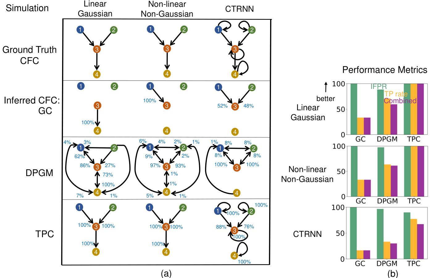
In the motifs and simulation paradigms that we consider, there are neurons and possible edges (including self-loops) per simulation resulting with total of possible edges across simulations. Figure 4 compares in detail the results for GC, DPGM and TPC in inference of true CFC for noise level and thresholding parameter . Here we also report the percentage of the simulations that has each estimated edge present. Higher percentage indicates higher confidence in the detection of that edge. Figure 5 compares the Combined Score of the approaches over different values of noise level and thresholding parameter for each simulation paradigm.
-
In Linear Gaussian scenario (left column in Figure 4), the connections between neurons in the Ground Truth CFC are excitatory due to positive coefficients in the linear dynamical equation for neural activity. GC generates a sparse set of edges in which it correctly detects a single edge among the three edges of the true CFC but misses two other edges. DPGM generates a large number of edges (9 out of 16), many of which are spurious, though it has a high percentage for expected edges in the Ground Truth CFC ( with and respectively). TPC obtains the Ground Truth CFC, with no spurious edges and obtains the expected edges in all of the trials ( with , and respectively). Overall, GC, DPGM and TPC produce , , and , and CS respectively. Thereby, among the three methods, we conclude that TPC detects the edges perfectly, while GC is highly specific to correct edges, but since it does not detect two out of three edges it is not as sensitive as DPGM.
-
In the Non-linear Non-Gaussian scenario (second column), in the Ground Truth CFC consists of excitatory due to being an increasing function, while is an inhibitory connection due to being a decreasing function for in the dynamical equation. As previously, GC consistently detects a sparse set of edges (single edge with ) which is one of the three true edges. DPGM again generates a large number of edges, some of which are spurious. In the majority of trials ( and , respectively), DPGM correctly obtains two of the three true edges and . In contrast, TPC obtains no spurious edges and the true edges were detected for all the trials (, , with ). In summary, GC, DPGM and TPC yielded and and CS . For this scenario, TPC again has the highest performance among the methods.
-
In CTRNN scenario (third column), self-loops are present for each neuron, and due to positive weights and increasing activation function in their dynamical equation, the connections in the Ground Truth CFC are excitatory. GC obtains two of the three true non-self edges for of the trials. DPGM detects spurious edges, but also infers the non-self true edges for of the trials. In comparison, TPC infers no spurious edges and all the self true edges for of the trials and non-self true edges and for of the trials. In summary, IFPR of GC, DPGM and TPC is and TPR is and CS is respectively. Among all methods, TPC has the highest TPR, followed by DPGM and lastly GC. Since GC does not detect any false edges, it has the highest IFPR, followed by DPGM and lastly TPC, though all of them have IFPR of at least . In terms of the CS, TPC has the highest performance compared to other methods.

We compare Combined Score of TPC and other approaches across varying levels of simulation noise from to and thresholding parameter in Figure 5. In the Linear Gaussian scenario, we note that TPC has a CS of across all levels of simulation noise and thresholding parameter , and is followed by DPGM in performance and lastly GC. In the Non-linear Non-Gaussian scenario, TPC has the highest CS compared to other methods across levels of noise and . In the CTRNN scenario, the performance of all the three approaches is lower compared to the other simulation paradigms for different level of and , yet TPC has higher CS compared to the other methods over the different parameter values.
We demonstrate the connectivity weights obtained by TPC and inferred nature of connections, whether excitatory or inhibitory, across simulations for noise level and thresholding parameter in Figure 6. In the Linear Gaussian scenario, the estimated connectivity weight of , , are , across simulation trials. Since the weights are positive, thereby the connections are labeled to be excitatory in all simulation trials, which agrees with the Ground Truth. In the Non-linear Non-Gaussian scenario, the estimated weight for the connection is in median and ranges between . Therefore the weight is always negative and labeled inhibitory in the simulation trials. The weight for are in median and ranges between and respectively. Their weights are always positive and labeled excitatory in all the simulation trials. These labels for the nature of connections obtained by TPC agrees with the ground truth. In the CTRNN scenario, the estimated connectivity weight for are in median respectively and ranges over positive values in all the simulation trials. Thereby the connections are labeled excitatory in all the simulations trials, which agrees with the Ground Truth.
5 Application to Benchmark Data
We applied TPC to find the CFC from datasets in the public benchmarking platform - CauseMe [47], and compared with benchmarked approaches in the platform in their performance to recover causal interactions present in the datasets. We used the River Runoff (real data) and Logistic Map (synthetic data) benchmarking datasets (See Appendix D). We compare the approaches PCMCI-GPDC [48], selVAR [49] - which are among the top of the leaderboard for performance on the benchmarking datasets, GC, DPGM (estimated by the PC algorithm), and TPC (Our).
| Combined [True, 1-False] Rates (%) | ||
|---|---|---|
| Algorithm | River-Runoff (Real) | Logistic Map (Synthetic) |
| GC | 37 [45, 92] | 79 [86, 93] |
| PCMCI | 45 [100, 45] | 86 [89, 97] |
| selVAR | 54 [91, 63] | 87 [88, 99] |
| DPGM | 60 [64, 96] | 19 [27, 92] |
| TPC (Our) | 72(+12%) [100, 72] | 84(-3%) [90, 94] |
As previously, we measured the performance of the algorithms using 1 - False Positive Rate (IFPR), True Positive Rate (TPR) and Combined Score given by Youden’s Index (CS = TPR - FPR) (See Table 1). The River Runoff dataset is comprised of contemporaneous interactions and is expected to demonstrate the performance of the methods in an empirical setting. The Logistic Map dataset is synthetic and excludes contemporaneous interactions and shows the performance of the methods when the ground truth connectivities are specifically controlled for.
In terms of CS, TPC has recorded the best performance with a score of , followed by DPGM, selVAR, PCMCI-GPDC and GC at respectively. TPC exceeds the second best approach by 12%. In terms of TPR, TPC and PCMCI have the highest scores at , followed by selVAR, DPGM and GC at respectively. In terms of IFPR, DPGM has the best performance with a score of closely followed by GC at , TPC at , and selVAR and PCMCI with . DPGM and GC turn out to have higher IFPR than TPC because they detect fewer false edges, but that is achieved by their detection of fewer edges altogether including fewer true edges leading to a low TPR. In contrast, TPC has greater sensitivity in detecting edges, whose benefit is that TPC detects all the true edges correctly leading to TPR. In terms of both TPR and IFPR, TPC maintains a better trade-off, and thereby a better CS compared to other methods.
For the logistic map dataset, in terms of CS, selVAR, PCMCI-GPDC and TPC have scores of respectively, followed by GC with and lastly DPGM with . In terms of TPR, TPC has the highest score of , followed by PCMCI, selVAR, GC and TPC with TPR of respectively, with DPGM having comparatively lowest TPR of . In terms of IFPR, all the approaches have a score of at least . Thereby, TPC achieves a high CS of , short of from the best CS by selVAR of .
The results indicate that in the real benchmark dataset of River-Runoff, TPC outperforms all methods by a substantial gap, whereas, in the synthetic benchmark dataset of Logistic Map, TPC has Combined Score of , being in the top group of CS performance. While selVAR and PCMCI achieve a CS of and respectively in the synthetic dataset, they achieve a low CS of and in the real dataset. Since the synthetic dataset is generated by a model controlling coupling strength between variables, low noise and devoid of contemporaneous interactions, thereby most of the methods including TPC perform fairly well in the range of . In contrast, in the real dataset, the coupling between variables as well as noise are not controlled and contemporaneous interactions are expected to be present as the sampling resolution is greater than the time taken for interactions between the variables. Thereby, the real dataset provides a challenge for the methods where TPC outperforms other approaches with a CS and shows significant improvement in performance than the other methods. Presence of TPC in top group of performance for both benchmarks indicates the generality and applicability of TPC to various scenarios.
6 Application to Neurobiological Data

We proceed and test the methods on neural data consisting of electrophysiological recordings in the Visual Coding Neuropixels dataset of the Allen Brain Observatory [50, 51]. We compare TPC with Granger Causality (GC) and Sparse Partial Correlation, that are popular methods for obtaining CFC and Associative Functional Connectivity (AFC) from electrophysiological neural recordings. The dataset consists of sorted spike trains and local field potentials recorded simultaneously from up to six cortical visual areas, hippocampus, thalamus, and other adjacent structures of mice, while the mice passively view a stimuli shown to them. The stimuli include static gratings, drifting gratings, natural scenes/images and natural movies, which are shown to the mice with repetitions. The data has been recorded from the neurons with the recently developed technology of Neuropixels which allows real-time recording from hundreds of neurons across the brain simultaneously by inserting multiple probes into the brain [52]. Details of the dataset are in Appendix E.
Figure 7 shows the adjacency matrices for the FC obtained by the methods for one trial in each of the stimuli categories. For each stimuli categories, the AFC constitutes a distinct pattern of connectivity among the neurons. It is expected that the CFC will be a directed subgraph of the AFC and be consistent with the overall patterns present in the AFC [53, 54]. However, the patterns present in the CFC obtained by GC do not match with the AFC. In contrast, the overall patterns present in the CFC obtained by TPC indeed match with the AFC. On a detailed level, there are differences between TPC-CFC and AFC: TPC results in a directed graph thereby its adjacency matrix is asymmetric while AFC is an undirected graph with symmetric adjacency matrix. Furthermore, the CFC obtained by TPC includes self-loops represented by the diagonals of the adjacency matrix and results in a sparse matrix devoid of noise since the connections passed conditional independence tests and bootstrap stability thresholds. In the CFC obtained by TPC (see Figure 7), a greater extent of connectivity within the active neurons in Primary Visual Cortex is evoked by natural scenes, in Posteromedial and Anteromedial Visual Cortex by static gratings, in Anterolateral Visual Cortex and Thalamus by full-field flashes, compared to other stimuli. All four stimuli exhibit distinct patterns of connectivity in the Cornu Ammonis regions of the Hippo-Campal Formation. Natural Scenes and Static gratings evoke more prominent connectivity within the Subiculum compared to other stimuli.
6.1 Graphical Comparison of Estimated CFC over Stimuli
To study the differences in functional connectivity between the stimuli categories, we investigate the topological patterns in the CFC estimated above. The topological patterns can be summarized by graph theoretic measures [55, 56, 57], as follows. The graph measures were computed using the Networkx Python library [58], over different trials of each stimuli.
- •
Betweenness centrality: the fraction of all shortest paths that pass through a node, averaged over nodes, indicating the average effect of individual nodes on information flow among the remaining network’s nodes.
- •
Transitivity: the fraction of all possible triangles present in the graph, indicating prevalence of clustered connectivity.
- •
Assortativity: measures the similarity of connections in the graph with respect to the node degree.
- •
Clustering Coefficient: the average of all clustering coefficients in the network, reflecting the tightness of connections between nodes.
- •
Global Efficiency: average inverse shortest path length, reflecting node’s ability to propagate information with other nodes in the graph.
- •
Local Efficiency: measures the global efficiency for the neighborhood of a node, averaged over nodes, indicating efficiency of transmitting information by nodes with their neighborhood in the graph.
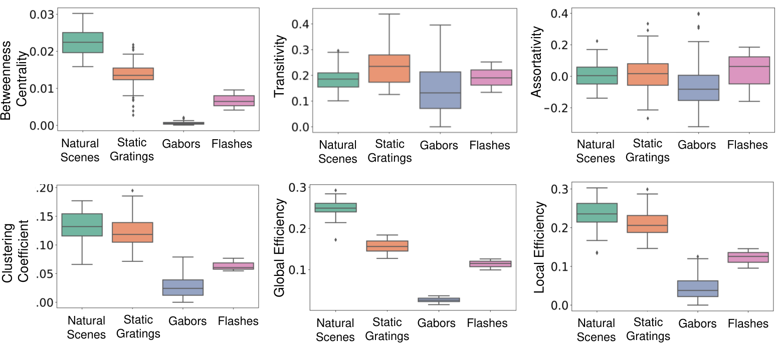
The results of the graph measures for different stimuli are summarized by boxplots. The boxplot of a graph measure (e.g. betweenness centrality) for a stimulus (e.g. natural scenes) shows the distribution of the values of the graph measure over trials for that stimulus, with the top and bottom of the box indicating the upper and lower quartiles of the distribution, the middle of the box indicating the median, while the whiskers extend to show the rest of the distribution excluding outliers, which are marked by points (See Figure 8).
In Figure 8, in terms of betweenness centrality, natural scenes have higher score compared to other stimuli, followed by static gratings, then flashes and lastly gabor patches. This shows that during natural scenes, the active neurons have a more remarkable effect on the neural information flow, compared to other stimuli, while gabor patches have the least remarkable effect. In terms of transitivity, the scores between the stimuli are close, though static gratings have a relatively higher transitivity, followed by natural scenes, flashes and gabors. This indicates that static gratings evoked a relatively higher prevalence of clustered connectivity, followed by natural scenes, flashes and lastly gabor patches. In terms of assortativity, the stimuli did not evoke a comparatively distinct score as well. In terms of clustering coefficient, natural scenes and static gratings have higher scores compared to flashes and gabors. This shows that, natural scenes and static gratings have the most tightness of connections between nodes in the graph, flashes have a comparatively lower tightness of connections, while gabor patches have the least score. In terms of global efficiency, natural scenes have the highest score, while, static gratings have comparatively lower score, followed by flashes and gabor patches. This shows that natural scenes evoked comparatively highest efficiency of information propagation in the CFC globally, followed by static gratings, flashes and gabors. In terms of local efficiency, the trend across stimuli is similar to global efficiency, while natural scenes and static gratings evoked a more similar local efficiency compared to global efficiency. This shows that the efficiency in information propagation in local neighborhoods of neurons is higher for natural scenes and static gratings to a similar extent, but with higher efficiency compared to flashes and gabor patches.
7 Discussion
In this paper, we propose a novel methodology, the TPC Algorithm, for finding causal functional connectivity between neurons from neural time series using Directed Probabilistic Graphical Models (DPGM). In particular, we extend the applicability of DPGM to CFC inference from time series by unrolling and implementing the Directed Markov Property (DMP) to obtain the unrolled DAG reflecting causal spatial and temporal interactions. We then roll the DAG back to obtain the CFC graph. The methodology exhibits interpretability of causal interactions over time between neural entities. It also incorporates time delays in interactions between neurons as well as the presence of feedback-loops. The model and the approach are non-parametric, meaning that it does not require the specification of a parametric dynamical equation for neural activity. We show that if the neural activity obeys an arbitrary dynamical process, the Rolled CFC-DPGM is consistent with respect to the causal relationships implied by the dynamical process. We determine that the Rolled CFC-DPGM is predictive of counterfactual queries such as ablation or modulation. We show that the answers can be provided by using simple causal reasoning with the edges of the rolled CFC-DPGM. We demonstrate the utilization of the methodology in obtaining CFC from simulations and compare the performance of TPC with other methods such as Granger Causality (GC) and common DPGM. Furthermore, we apply the methods to benchmarks of time-series causal inference and neurobiological dataset from mice brain presented with various visual stimuli. The results provide insights into the CFC between neurons in the mouse brain in a variety of stimuli scenario. We also compare the topological patterns in the estimated CFC between different stimuli using graph-theoretic measures.
| GC | DCM | DPGM | TPC | |
|---|---|---|---|---|
| Form of Causality | Non-zero parameters in VAR model | Coupling parameters in biological model | Directed Markov Graph | Directed Markov Graph over time-delayed variables |
| Inclusion of temporal relationships | Yes | Yes | No, formulation for static variables | Yes, adapts DPGM for inter-temporal relationships |
| Inclusion of contemporaneous relationships | No | Yes, by a differential equation | No | Yes, if then . |
| Generalizable Statistical Model | Yes | No | Yes | Yes |
| Non-parametric Model | Yes, parametric and non-parametric approaches exist. | No, biologically mechanistic non-linear model. | Yes, equivalent to an arbitrary functional relationship between nodes. | Yes, equivalent to an arbitrary functional relationship between neural activity at different times. |
| Supports CFC Inference | Yes | No, suitable for comparing model hypotheses | Yes | Yes |
| Cycles (including self-loops) Occuring In The Model | Yes for VAR model (neuron when for some ). | Yes ( when ) | No, it is a DAG | Yes ( when for some ) |
| Incorporation of Interventional and Counterfactual queries | No | No | Yes but for static variables. | Yes, adapts for temporal scenario, can predict the consequence on CFC of counterfactual intervention to neural activity. |
The distinctive and useful aspect of TPC is that it takes into consideration neural interactions over time. In neuroscience literature, causality is typically referred to as “a cause of an observed neural event (the ‘effect’) as a preceding neural event whose occurrence is necessary to observe the effect” [2]. The approach of unrolling causal graphs over time and considering time-delays in TPC incorporates this definition by essentially finding whether the previous time values of the neurons impact the present value of a particular neuron by the obtained directed graph. By virtue of the Directed Markov Property, TPC incorporates causality of neural interactions in a non-parameteric, model-free manner and incorporates interventional properties. The bootstrapping step filters spurious connections by repeating the inference of CFC over several subsampled blocks of the time series and discarding those connections that are absent in multiple repetitions. Pruning further selects edges by discarding edges with exceedingly low edge weight. In contrast, parametric approaches, such as GC, do not satisfy the Directed Markov Property, thereby not incorporating interventional properties. Furthermore, in comparative studies with simulated, benchmark and real neurobiological datasets, we found the performance of TPC to be better compared to other approaches. We conclude by summarizing, in Table 2, the differences and benefits of TPC in a comparison with other approaches including variants of the PC algorithm (DPGM) which satisfy DMP in a static data setting, and other approaches that do not obey the DMP, such as Granger Causality (GC) and Dynamic Causal Model (DCM), outlining their strengths and weaknesses with respect to several criteria of causality in functional connectomics. Indeed, capturing as many causal criteria is fundamental to any approach from statistical and application points of view.
Our exposition of properties of each approach and the comparative study show that each of the methods address different aspects of modeling causality of neural interaction and mapping them in the form of a graph [6]. The comparative table demonstrates that with respect to the model that each approach is assuming, GC requires a linear model in its common use, though recent non-linear and non-parametric extensions, have been applied. DCM requires a strict well defined mechanistic biological model and thus can only compare different models based on evidence from data. In comparison, DPGM and TPC have the advantage of not requiring modeling of the neural dynamics using a parametric equation or assumption of a linear model. While DPGM is developed for static variables, and as such cannot address temporal and contemporaneous relationships and must obey DAG architechture, TPC is suited for time series setting and extends DPGM for spatiotemporal data. TPC obtains the CFC that follows Directed Markov Property extended to include inter-temporal relationships in a time-series setting such that parent-child relations between neurons are equivalent to arbitrary functional relationships between their neural activity over time. In terms of incorporating contemporaneous interactions arising when causal interactions happen faster than sampling rate, while GC and DPGM do not, TPC is able to incorporate contemporaneous interactions by design. In terms of incorporating self-loops in neural activity, while DPGM typically produces a DAG, TPC incorporates self-loops in neural activity. In regards to guarantee of causality, GC can provide useful insights into a system’s dynamical interactions in different conditions, however its causal interpretation is not guaranteed as it focuses on the predictability of future based on past observations of variables. DCM uses the parameters for coupling between hidden neural states in competing biological models to indicate CFC, however it compares hypothetical models based on evidence from data which relevance to causality is not guaranteed (Friston et al., 2003). In summary, TPC extends DPGM to the time-series setting and provides a probabilistic foundation for causality which is predictive of the consequence of possible intervention like neuron ablation and neuromodulation.
While TPC provides a powerful causal framework for time series, its current version relies on the PC algorithm which in turn assumes causal sufficiency, that is, all the causes of the input variables are present within the input variables. In the presence of latent confounders, the PC can lead to spurious edges. These are partly remediated by the TPC Algorithm by discarding spurious edges in the Bootstrap and Pruning steps, but some of these effect may remain. To address this, an alternative strategy that could be considered is replacing the PC algorithm with the FCI algorithm in Step 3 of TPC (1) since the FCI algorithm exhibits statistical consistency, that converges in probability to the true causal relationships, given i.i.d. samples in the presence of latent confounders [33]. However, the FCI algorithm identifies indirect connections only and not direct connections, thereby would result in a CFC with indirect causal connections.
Under the assumptions of 1) causal sufficiency, 2) faithfulness, and 3) given i.i.d. samples, the PC algorithm’s estimated causal DAG is statistically consistent. In light of these assumptions, the step 2 of the TPC algorithm constructs samples with a time-delay of between samples from a bootstrap window, for max time-delay of interaction , which are used as an input to the PC algorithm in the next step. The time-delay between samples of reduces between-sample dependence. And, the samples being constructed from a short bootstrap window instead of the entire time series aids to make their distribution fairly identical. Yet, specifications of of lower value could lead to between-sample dependence and rapid perturbations to the time series in a bootstrap window can lead to distribution changes between samples in a bootstrap window, leading to potential reduction in efficacy of edge detection by the PC algorithm. To improve overall efficacy in such scenarios and curb spurious edge detections, the bootstrap step of the TPC algorithm outputs many CFCs over random time windows and preserves only stable edges over the set of CFCs. In the pruning step, the edges in the CFC are pruned if having an exceedingly low connectivity weight.
In conclusion, TPC provides a probabilistic and interpretable formulation for CFC modeling and inference in the context of neural time series. We have established the statistical properties of the model as well as demonstrated its performance in estimation of CFC. We have demonstrated TPC application in continuous time series datasets, however TPC is similarly applicable to discrete time series datasets by simply using a statistical conditional independence test for discrete data in the algorithm. This can be especially relevant for count datasets such as spiking neuron datasets.
References
- [1] R Clay Reid. From functional architecture to functional connectomics. Neuron, 75(2):209–217, 2012.
- [2] Andrew T Reid, Drew B Headley, Ravi D Mill, Ruben Sanchez-Romero, Lucina Q Uddin, Daniele Marinazzo, Daniel J Lurie, Pedro A Valdés-Sosa, Stephen José Hanson, Bharat B Biswal, et al. Advancing functional connectivity research from association to causation. Nature neuroscience, 1(10), 2019.
- [3] Jessica M Cassidy, Jasper I Mark, and Steven C Cramer. Functional connectivity drives stroke recovery: shifting the paradigm from correlation to causation. Brain, 2021.
- [4] Ruben Sanchez-Romero and Michael W Cole. Combining multiple functional connectivity methods to improve causal inferences. Journal of cognitive neuroscience, 33(2):180–194, 2021.
- [5] Emily S Finn, Xilin Shen, Dustin Scheinost, Monica D Rosenberg, Jessica Huang, Marvin M Chun, Xenophon Papademetris, and R Todd Constable. Functional connectome fingerprinting: identifying individuals using patterns of brain connectivity. Nature neuroscience, 18(11):1664–1671, 2015.
- [6] Rahul Biswas and Eli Shlizerman. Statistical perspective on functional and causal neural connectomics: A comparative study. Frontiers in Systems Neuroscience, 16, 2022.
- [7] Maksim G Sharaev, Viktoria V Zavyalova, Vadim L Ushakov, Sergey I Kartashov, and Boris M Velichkovsky. Effective connectivity within the default mode network: dynamic causal modeling of resting-state fmri data. Frontiers in human neuroscience, 10:14, 2016.
- [8] Steffen L Lauritzen. Causal inference from graphical models. Complex stochastic systems, pages 63–107, 2001.
- [9] Marloes Maathuis, Mathias Drton, Steffen Lauritzen, and Martin Wainwright. Handbook of graphical models. CRC Press, 2018.
- [10] Ana María Estrada Gómez, Kamran Paynabar, and Massimo Pacella. Functional directed graphical models and applications in root-cause analysis and diagnosis. Journal of Quality Technology, pages 1–17, 2020.
- [11] Daniel Felix Ahelegbey. The econometrics of bayesian graphical models: a review with financial application. Journal of Network Theory in Finance, 2(2):1–33, 2016.
- [12] Imme Ebert-Uphoff and Yi Deng. Causal discovery for climate research using graphical models. Journal of Climate, 25(17):5648–5665, 2012.
- [13] Markus Kalisch, Bernd AG Fellinghauer, Eva Grill, Marloes H Maathuis, Ulrich Mansmann, Peter Bühlmann, and Gerold Stucki. Understanding human functioning using graphical models. BMC Medical Research Methodology, 10(1):1–10, 2010.
- [14] Ke Deng, Delin Liu, Shan Gao, and Zhi Geng. Structural learning of graphical models and its applications to traditional chinese medicine. In International Conference on Fuzzy Systems and Knowledge Discovery, pages 362–367. Springer, 2005.
- [15] Michael S Haigh and David A Bessler. Causality and price discovery: An application of directed acyclic graphs. The Journal of Business, 77(4):1099–1121, 2004.
- [16] Huange Wang, Fred A van Eeuwijk, and Johannes Jansen. The potential of probabilistic graphical models in linkage map construction. Theoretical and Applied Genetics, 130(2):433–444, 2017.
- [17] Christine Sinoquet. Probabilistic graphical models for genetics, genomics, and postgenomics. OUP Oxford, 2014.
- [18] Raphaël Mourad, Christine Sinoquet, and Philippe Leray. Probabilistic graphical models for genetic association studies. Briefings in bioinformatics, 13(1):20–33, 2012.
- [19] Junbai Wang, Leo Wang-Kit Cheung, and Jan Delabie. New probabilistic graphical models for genetic regulatory networks studies. Journal of biomedical informatics, 38(6):443–455, 2005.
- [20] Hexuan Liu, Jimin Kim, and Eli Shlizerman. Functional connectomics from neural dynamics: probabilistic graphical models for neuronal network of caenorhabditis elegans. Philosophical Transactions of the Royal Society B: Biological Sciences, 373(1758):20170377, 2018.
- [21] Nir Friedman. Inferring cellular networks using probabilistic graphical models. Science, 303(5659):799–805, 2004.
- [22] Peter Spirtes, Clark N Glymour, Richard Scheines, and David Heckerman. Causation, prediction, and search. MIT press, 2000.
- [23] Judea Pearl. Causality. Cambridge university press, 2009.
- [24] Ila R Fiete, Walter Senn, Claude ZH Wang, and Richard HR Hahnloser. Spike-time-dependent plasticity and heterosynaptic competition organize networks to produce long scale-free sequences of neural activity. Neuron, 65(4):563–576, 2010.
- [25] Mohammad R Arbabshirani, Adrian Preda, Jatin G Vaidya, Steven G Potkin, Godfrey Pearlson, James Voyvodic, Daniel Mathalon, Theo van Erp, Andrew Michael, Kent A Kiehl, et al. Autoconnectivity: A new perspective on human brain function. Journal of neuroscience methods, 323:68–76, 2019.
- [26] Roman Borisyuk and Frank Hoppensteadt. Oscillatory models of the hippocampus: a study of spatio-temporal patterns of neural activity. Biological cybernetics, 81(4):359–371, 1999.
- [27] Michael J Jutras and Elizabeth A Buffalo. Synchronous neural activity and memory formation. Current opinion in neurobiology, 20(2):150–155, 2010.
- [28] Thomas S Richardson, Peter Spirtes, et al. Automated discovery of linear feedback models. Carnegie Mellon [Department of Philosophy], 1996.
- [29] Kenneth A Bollen. Structural equations with latent variables wiley. New York, 1989.
- [30] Mathias Drton and Marloes H Maathuis. Structure learning in graphical modeling. Annual Review of Statistics and Its Application, 4:365–393, 2017.
- [31] Markus Kalisch and Peter Bühlmann. Estimating high-dimensional directed acyclic graphs with the pc-algorithm. Journal of Machine Learning Research, 8(Mar):613–636, 2007.
- [32] Robert E Tillman, Arthur Gretton, and Peter Spirtes. Nonlinear directed acyclic structure learning with weakly additive noise models. In NIPS, pages 1847–1855. Citeseer, 2009.
- [33] Peter Spirtes, Christopher Meek, and Thomas Richardson. An algorithm for causal inference in the presence of latent variables and selection bias. Computation, causation, and discovery, 21:1–252, 1999.
- [34] Jiji Zhang and Peter L Spirtes. Strong faithfulness and uniform consistency in causal inference. arXiv preprint arXiv:1212.2506, 2012.
- [35] Norman R Swanson and Clive WJ Granger. Impulse response functions based on a causal approach to residual orthogonalization in vector autoregressions. Journal of the American Statistical Association, 92(437):357–367, 1997.
- [36] Jakob Runge, Sebastian Bathiany, Erik Bollt, Gustau Camps-Valls, Dim Coumou, Ethan Deyle, Clark Glymour, Marlene Kretschmer, Miguel D Mahecha, Jordi Muñoz-Marí, et al. Inferring causation from time series in earth system sciences. Nature communications, 10(1):1–13, 2019.
- [37] Shigeru Shinomoto. Estimating the firing rate. In Analysis of Parallel Spike Trains, pages 21–35. Springer, 2010.
- [38] Ian H Stevenson, James M Rebesco, Lee E Miller, and Konrad P Körding. Inferring functional connections between neurons. Current opinion in neurobiology, 18(6):582–588, 2008.
- [39] Klaas Enno Stephan, Nikolaus Weiskopf, Peter M Drysdale, Peter A Robinson, and Karl J Friston. Comparing hemodynamic models with dcm. Neuroimage, 38(3):387–401, 2007.
- [40] Caitlin Mullins, Gord Fishell, and Richard W Tsien. Unifying views of autism spectrum disorders: a consideration of autoregulatory feedback loops. Neuron, 89(6):1131–1156, 2016.
- [41] Julia M Sheffield and Deanna M Barch. Cognition and resting-state functional connectivity in schizophrenia. Neuroscience & Biobehavioral Reviews, 61:108–120, 2016.
- [42] Judea Pearl et al. Causal inference in statistics: An overview. Statistics surveys, 3:96–146, 2009.
- [43] Marloes H Maathuis, Markus Kalisch, Peter Bühlmann, et al. Estimating high-dimensional intervention effects from observational data. The Annals of Statistics, 37(6A):3133–3164, 2009.
- [44] Yimin Huang and Marco Valtorta. Pearl’s calculus of intervention is complete. arXiv preprint arXiv:1206.6831, 2012.
- [45] Ana-Maria Šimundić. Measures of diagnostic accuracy: basic definitions. Ejifcc, 19(4):203, 2009.
- [46] Jørgen Hilden and Paul Glasziou. Regret graphs, diagnostic uncertainty and youden’s index. Statistics in medicine, 15(10):969–986, 1996.
- [47] Bart Bussmann, Jannes Nys, and Steven Latré. Neural additive vector autoregression models for causal discovery in time series. In International Conference on Discovery Science, pages 446–460. Springer, 2021.
- [48] Jakob Runge, Peer Nowack, Marlene Kretschmer, Seth Flaxman, and Dino Sejdinovic. Detecting and quantifying causal associations in large nonlinear time series datasets. Science Advances, 5(11):eaau4996, 2019.
- [49] Sebastian Weichwald, Martin E. Jakobsen, Phillip B. Mogensen, Lasse Petersen, Nikolaj Thams, and Gherardo Varando. Causal structure learning from time series: Large regression coefficients may predict causal links better in practice than small p-values. In Hugo Jair Escalante and Raia Hadsell, editors, Proceedings of the NeurIPS 2019 Competition and Demonstration Track, volume 123 of Proceedings of Machine Learning Research, pages 27–36. PMLR, 08–14 Dec 2020.
- [50] Saskia EJ de Vries, Jerome A Lecoq, Michael A Buice, Peter A Groblewski, Gabriel K Ocker, Michael Oliver, David Feng, Nicholas Cain, Peter Ledochowitsch, Daniel Millman, et al. A large-scale standardized physiological survey reveals functional organization of the mouse visual cortex. Nature Neuroscience, 23(1):138–151, 2020.
- [51] Allen-Brain-Observatory. Allen institute for brain science. Available from: https://portal.brain-map.org/explore/circuits/visual-coding-neuropixels, October, 2019.
- [52] James J Jun, Nicholas A Steinmetz, Joshua H Siegle, Daniel J Denman, Marius Bauza, Brian Barbarits, Albert K Lee, Costas A Anastassiou, Alexandru Andrei, Çağatay Aydın, et al. Fully integrated silicon probes for high-density recording of neural activity. Nature, 551(7679):232–236, 2017.
- [53] Mehrdad Dadgostar, Seyed Kamaledin Setarehdan, Sohrab Shahzadi, and Ata Akin. Functional connectivity of the pfc via partial correlation. Optik, 127(11):4748–4754, 2016.
- [54] Yikai Wang, Jian Kang, Phebe B Kemmer, and Ying Guo. An efficient and reliable statistical method for estimating functional connectivity in large scale brain networks using partial correlation. Frontiers in neuroscience, 10:123, 2016.
- [55] Olaf Sporns, Dante R Chialvo, Marcus Kaiser, and Claus C Hilgetag. Organization, development and function of complex brain networks. Trends in cognitive sciences, 8(9):418–425, 2004.
- [56] Martijn P van den Heuvel, Cornelis J Stam, Maria Boersma, and HE Hulshoff Pol. Small-world and scale-free organization of voxel-based resting-state functional connectivity in the human brain. Neuroimage, 43(3):528–539, 2008.
- [57] Issei Ueda, Shingo Kakeda, Keita Watanabe, Koichiro Sugimoto, Natsuki Igata, Junji Moriya, Kazuhiro Takemoto, Asuka Katsuki, Reiji Yoshimura, Osamu Abe, et al. Brain structural connectivity and neuroticism in healthy adults. Scientific reports, 8(1):1–8, 2018.
- [58] Aric Hagberg, Pieter Swart, and Daniel S Chult. Exploring network structure, dynamics, and function using networkx. Technical report, Los Alamos National Lab.(LANL), Los Alamos, NM (United States), 2008.
- [59] Ariel Rokem, M Trumpis, and F Perez. Nitime: time-series analysis for neuroimaging data. In Proceedings of the 8th Python in Science Conference, pages 68–75, 2009.
- [60] Christoph Schmidt, Britta Pester, Nicole Schmid-Hertel, Herbert Witte, Axel Wismüller, and Lutz Leistritz. A multivariate granger causality concept towards full brain functional connectivity. PloS one, 11(4):e0153105, 2016.
Appendix A Proof of Theorem 1
Let , , and . Rewriting Eq. (5) we get,
By Theorem 1.4.1 in [23], the above implies that satisfies the DPM with respect to .
Therefore by Definition 1, the rolled CFC-DPGM, , has nodes and edges given by , since , for and . That is, .
Appendix B Proof of Theorem 2
During the experimental/counterfactual intervention, such as controlling the activity of neuron or neuron ablation, the activity would no longer be a function of the activities of the neurons at preceding time points for , while the activity of neurons which are not intervened, would still be a function of activity at preceding time points. That is, , for and for for , where represents the distribution of neural activity due to the experimental intervention. For example, is identically for neuron ablation, and can be an oscillating function with a high amplitude and random noise for stimulation through external control. The dynamics can be written as
| (6) |
for , where for and , where denotes the null set. In other words, has all connections same as except that all connections directing to the intervened neurons are removed. It follows from Eq. (6) and Theorem 1 that is the causal functional connectivity between the neurons in during time when are subject to experimental intervention.
For ablations,the edges originating from , can be removed since the activity of these neurons would be fixed (at zero) and would be trivial variables that can be excluded from the argument of the function in Eq. (6).
Appendix C Simulation Study Details
We study the following simulation paradigms.
- 1.
Linear Gaussian Time Series (Figure 4a left-column). Let denote a Normal random variable with mean and standard deviation . We define as a linear Gaussian time series for whose true CFC has the edges . Let for , and for ,
We obtain 25 simulations of the entire time series each for different noise levels .
- 2.
Non-linear Non-Gaussian Time Series (Figure 4a middle-column). Let denote a Uniformly distributed random variable on the interval . We define as a non-linear non-Gaussian time series for whose true CFC has the edges . Let for and for ,
We obtain 25 simulations of the entire time series each for different noise levels .
- 3.
Continuous Time Recurrent Neural Network (CTRNN) (Figure 4a right-column). We simulate neural dynamics by Continuous Time Recurrent Neural Networks, Eq. (7). is the instantaneous firing rate at time for a post-synaptic neuron , is the linear coefficient to pre-synaptic neuron ’s input on the post-synaptic neuron , is the input current on neuron at time , is the time constant of the post-synaptic neuron , with being indices for neurons with being the total number of neurons. Such a model is typically used to simulate neurons as firing rate units,
(7) We consider a motif consisting of neurons with and otherwise. We also note that in Eq. 7, activity of each neuron depends on its own past. Therefore, the true CFC has the edges . The time constant is set to 10 msecs for each neuron . We consider to be distributed as independent Gaussian process with the mean of 1 and the standard deviation of . The signals are sampled at a time gap of msecs for a total duration of msecs. We obtain 25 simulations of the entire time series each for different noise levels .
The GC graph is computed using the Nitime Python library, which fits an MVAR model followed by using the GrangerAnalyzer to compute the Granger Causality [59]. The PC algorithm, which requires several samples of a scalar-valued random variable (measured activity) for neurons , is used to compute DPGM. We define as a windowed average of recordings over a duration of msec: , and averaging over different msec windows with a gap of msec between consecutive windows yields different samples. This choice of performs better than considering to be neural recordings at time : , with different giving different samples of in previous work [6]. The TPC algorithm computes the rolled CFC-DPGM directly from the signals and, we use a maximum time-delay of interaction of msec.
The choice of thresholds tunes the decision whether a connection exists in the CFC. For DPGM and TPC, increasing the significance level for conditional independence tests increases the rate of detecting edges, but also increasing the rate of detecting false positives. We consider for DPGM and TPC. For GC, a likelihood ratio statistic is obtained for testing for . An edge is outputted if has a value greater than a threshold. We use a percentile-based threshold, and output an edge if is greater than percentile of ’s over all pairs of neurons in the graph [60]. We consider which corresponds to percentile thresholds of . For the bootstrap procedure in TPC, we consider 50 bootstrap iterations with bootstrap window length of msec and bootstrap stability cutoff .
Appendix D Benchmark Datasets
We use the following benchmark datasets from Causeme [36, 47].
- 1.
River Runoff. This is a real dataset that consists of time series of river runoff at different stations. The time series have a daily time resolution and only include summer months (June-August). The physical time delay of interaction (as inferred from the river velocity) are roughly below one day, hence the dataset has contemporaneous time interactions. This dataset has 12 variables and 4600 time recordings for each variable.
- 2.
Logistic Map. This is a synthetic dataset generated from logistic map with maximum time delay of 3 and a low dynamical noise and moderate strength of coupling between the variables. This dataset has 5 variables and 300 time recordings per variable.
The PC algorithm is used to compute the DPGM from the scalar-valued random variables , defined by the average of recordings of a time window of length , and averaging over alternate time windows of length and a gap of between consecutive windows results in samples of . Considering river runoff has large number of time recordings while logistic map has only recordings, we used and for river runoff and logistic map data respectively. The PC algorithm was implemented with p-value of for kernel-based non-linear conditional independence tests. In river-runoff and logistic map data, the TPC algorithm was implemented with maximum time-delay of interaction to be and recordings respectively, as per specification in the datasets, and a significance level for kernel-based conditional independence tests. For the bootstrap procedure in TPC, 50 bootstrap iterations with bootstrap window length of recordings and bootstrap stability threshold for river-runoff and logistic map datasets respectively.
Appendix E Visual Coding Neuropixels Dataset
For the purpose of application and comparison of the results of the methods discussed in this paper, we restrict our analysis to a 116 days old male mouse (Session ID 791319847) with 555 neurons whose spike trains are recorded simultaneously by six Neuropixel probes. The spike trains during the entire experiment were recorded at a frequency of KHz. We analyze the spike trains for four stimuli categories:
- 1.
Natural scenes, consisting of 118 natural scenes selected from three databases (Berkeley Segmentation Dataset, van Hateren Natural Image Dataset and McGill Calibrated Colour Image Database), with each scene presented briefly for 250ms and then replaced with the next scene image. Each scene is repeated 50 times in random order with intermittent blank intervals.
- 2.
Static gratings consisting of full-field sinusoidal gratings with 6 orientations (the angle of the grating), 5 spatial frequencies (the width of the grating), and 4 phases (the position of the grating) resulting in 120 stimulus conditions. Each grating is presented briefly (250 ms) before being replaced with a different orientation, spatial frequency and phase condition and each condition is repeated 50 times, in random order with intermittent blank intervals.
- 3.
Gabor patches with 3 orientations where the patch center is lying at one of the points in a visual field. Each gabor patch is being presented for 250ms and then replaced by a different patch, and each condition is repeated 50 times in random order with intermittent blank intervals.
- 4.
Full-field flashes, lasting for 250 ms followed by a blank interval of 1.75 s, and then the next flash, totaling 150 repetitions.
This variety of stimuli is ranging from relatively natural stimuli invoking mice’s natural habitats (natural scenes) to artificial stimuli (static gratings, gabors and flashes). Among the artificial stimuli, static gratings incorporate sinusoidal patches, while full-field flashes incorporate sharp changes in luminosity in the whole visual field in short period of time, and gabor patches incorporate sinusoidal patches with declining luminosity with distance from the center of the patch. With this choice of four stimuli we investigate how the variety of stimuli possibly invokes distinct patterns of neuronal interactions and connectivity. We exclude dynamic stimuli like natural movies, and drifting gratings, from this analysis because their results would require more nuanced study and interpretation, which we defer for future analysis.
Preprocessing
We convert the spike trains recorded at 1 KHz to bin size of 10 ms by aggregating and then separating by start and end times of each stimuli presentation and obtain the Peri-Stimulus Time Histograms (PSTH) with bin-size 10 ms. We smooth the PSTHs by a Gaussian smoothing kernel of bandwidth ms which provides a smoothed version of the PSTH for each neuron and each stimulus presentation. Some examples of the smoothed PSTH are displayed in Figure 7. We use the smoothed PSTHs for neurons over each stimuli type as input for inference of the FC between the neurons for each stimuli presentation. For each stimulus presentation, we first selected the set of neurons that were active in at least of the bins in the PSTH, and then collected the set of unique neurons over all stimuli, which resulted in 54, 43, 19 and 36 active neurons for natural scenes, static gratings, gabor patches and flashes respectively, and 68 unique active neurons overall. We considered separated the entire duration of stimulus presentation to yield 58 trials of natural scenes, 60 trials of static gratings, 58 trials of gabor patches, and, 3 trials of flashes, where each trial is of duration 7.5 s.
We compare TPC with two popular methods for inferring the FC from neural signals: Granger Causality (GC) and Sparse Partial correlation via Graphical Lasso penalized Maximum Likelihood Estimation (Sparse Partial Corr). The TPC algorithm was implemented with maximum time-delay of interaction 10 ms, significance level , bootstrap iterations, ms bootstrap window width, and stability threshold . For GC, we consider VAR model of order , and GC likelihood ratio statistic of greater than percentile as indicating edges [60]. For Sparse Partial Corr, the optimal penalization was determined by -fold cross-validation. A summary of the results is provided in Figure 7.