Reducing Model Churn: Stable Re-training of Conversational Agents
Abstract
Retraining modern deep learning systems can lead to variations in model performance even when trained using the same data and hyper-parameters by simply using different random seeds. This phenomenon is known as model churn or model jitter. This issue is often exacerbated in real world settings, where noise may be introduced in the data collection process. In this work we tackle the problem of stable retraining with a novel focus on structured prediction for conversational semantic parsing. We first quantify the model churn by introducing metrics for agreement between predictions across multiple re-trainings. Next, we devise realistic scenarios for noise injection and demonstrate the effectiveness of various churn reduction techniques such as ensembling and distillation. Lastly, we discuss practical trade-offs between such techniques and show that co-distillation provides a sweet spot in terms of churn reduction with only a modest increase in resource usage.
1 Introduction
Deep learning systems can perform inconsistently across multiple runs, even when trained on the same data with the same hyper-parameters. Deployment in real-world environments presents a challenge, where constantly changing production systems require frequent re-training of models. For a conversational semantic parsing system such as Google Assistant or Amazon Alexa, where the goal is to convert users’ commands into executable forms, this erratic behavior can have some unfortunate practical consequences. Some examples include irreproducibility, which limits the ability to make meaningful comparisons between experiments Dodge et al. 2019; Dodge et al. 2020, bias, which creates credibility issues if systems consistently struggle with members of a certain class D’Amour et al. 2020, and user frustration, which can arise due to unpredictable interactions over time.
The root cause of widely divergent behavior is underspecification D’Amour et al. 2020, where there are many equivalent but distinct solutions to a problem. Non-determinism in model training (e.g. different data orders or weight initializations) can lead to finding local minima that obtain the same measurements on a held-out test set but make different predictions (also known as model churn).
| Query | will i need snow tires to drive the sierra nevada mountains this afternoon? |
|---|---|
| Model Run 1 | [in:get_weather [sl:weather_attribute snow tires ] [sl:location sierra mountains ] [sl:date_time this afternoon ] ] |
| Model Run 2 | [in:get_info_road_condition [sl:road_condition snow tires ] [sl:location sierra mountains ] [sl:date_time this afternoon ] ] |
Even in an academic setting, controlling for all non-determinism is unrealistic - Table 1 provides an example of churn from the TOPv2 dataset Chen et al. 2020a. In this case, re-training the same model twice with the same data and hyper-parameters results in two different predictions for the given query. While at the token level the slots and arguments overlap, the intents are different, resulting in a drastically different user experience. In this scenario, the dataset is static and yet we still observe model churn. In a real-world setting, the dataset may be constantly changing and noisy, necessitating frequent re-training. The goal, then, is to maintain consistency even in this scenario.
We thus conduct experiments to evaluate and reduce churn across multiple model re-training runs. Our contributions are as follows:
- 1.
We extend the notion of model churn to structured prediction. To this end, we introduce new metrics for agreement and exact match agreement (Section 3).
- 2.
We show that techniques such as ensembling Dietterich 2000 and distillation/co-distillation Hinton et al. 2015; Kim and Rush 2016; Anil et al. 2018, described in Section 4, reduce churn on the TOP Gupta et al. 2018, TOPv2 Chen et al. 2020a, MTOP Li et al. 2021, and SNIPS Coucke et al. 2018 datasets (Section 6).
- 3.
We explore the effects of model churn in ‘‘real-world’’ environments, conducting experiments with a smaller model and two types of simulated noise (random and systematic)11 1 Datasets can be found at https://github.com/google/stable-retraining-conversational-agents to represent various sources of error (Sections 5 and 6).
- 4.
We make practical recommendations based on resource usage (number of parameters) in addition to accuracy and agreement and observe that co-distillation with label smoothing provides the best tradeoff (Section 7).
To the best of our knowledge, we are the first to study model churn for the structured prediction task of spoken language understanding (SLU).
2 Background and Related Work
The problem of model churn Milani Fard et al. 2016, defined as the difference in predictions observed across runs when re-training models, has traditionally been studied for classification tasks. In contrast with previous work, we study the problem of model churn for structured prediction, specifically for SLU. Shamir and Coviello 2020 introduced “anti-distillation” to increase diversity in ensemble predictions and Shamir et al. 2020 introduced the smooth-relu activation function; however, in our initial experiments we did not find significant improvement using these methods when applied to structured prediction. Other work has explored forms of smoothing to reduce churn, either by computing soft labels using the nearest neighbors Bahri and Jiang 2021 or by weighting the loss term of individual examples using the predicted probabilities from a teacher model Jiang et al. 2022. As these methods were developed for classification, we leave the task of adapting them to structured prediction for future work.
Other research has focused on related problems such as reproducibility McCoy et al. 2020 and calibration Guo et al. 2017; Mosbach et al. 2021. Nie et al. 2020 argue that this phenomenon is due to underlying task complexity and annotator disagreement. D’Amour et al. 2020 claim that reproducibility is primarily due to underspecification, where there are many distinct solutions to the same problem. While these problems are related to churn, both reproducibility and calibration metrics are computed relative to a target, rather than accounting for agreement across re-training runs.
It has been well known that ensembling increases reproducibility and model calibration Hansen and Salamon 1990; Lakshminarayanan et al. 2017. Since ensembles increase inference times, distillation Hinton et al. 2015 is commonly used to train a student model with similar inference resource usage. Reich et al. 2020 show that ensemble distillation improves calibration for machine translation and named entitity recognition. For our distillation baselines, we follow the recipe by Chen et al. 2020b. For co-distillation, we follow the recipe developed by Anil et al. 2018. In our work, we look at the aforementioned approaches and compare them in terms of resource usage, churn reduction, and effectiveness on the task of conversational semantic parsing Gupta et al. 2018; Cheng et al. 2020; Damonte et al. 2019; Aghajanyan et al. 2020; Lialin et al. 2020.
3 Task Definition and Evaluation
We follow recent work Rongali et al. 2020 and treat conversational semantic parsing as sequence generation using auto-regressive neural models. The goal is to make a structured prediction given a user command such as the example in Table 1. For structured prediction, the task of churn reduction is, given an input, to predict the exact same sequence across multiple re-training runs. A re-training run refers to the model parameters that result from different random weight initialization and data order but the same data and hyper-parameters.
Our aim is to reduce churn across runs while maintaining high accuracy on the gold labels. Thus, we report exact match accuracy (EM) with the mean over runs. While our goal is not to obtain the state of the art, we do want to show which methods reduce churn without a loss in performance.
To measure churn, we need a way to compare predictions across runs, independent of the gold labels. While previous work Shamir et al. 2020 has used metrics such as prediction difference (similar to Hamming distance), the focus was on classification tasks only, making it necessary to compute an alternative measure. Metrics such as edit distance or multiple sequence alignment would be appropriate for sequence generation tasks such as machine translation or paraphrasing, where churn across output may differ locally by only a few tokens. Comparatively, the meaning of these metrics is unclear for structured prediction tasks such as semantic parsing. For example, computing a token-level distance between a prediction such as “[in:unsupported ]” and “[in:get_event [sl:date_time this weekend ] ]” would not be a useful measure. Thus, we report sequence-level model agreement (AGR) across runs, where each example has a score of 1 if all runs agree on the exact same predicted sequence and 0 otherwise. However, it is possible for all runs to agree but make an incorrect prediction; the goal ultimately is to consistently make correct predictions. Consequently, we further extend this metric to include the case where the predictions from all runs agree and the predictions match the target. We refer to this metric as exact match agreement (EM@N).
4 Methods for Churn Reduction
For our experiments, we explore three techniques which have been effective on related problems such as model calibration: ensembling, which combines the predictions of multiple models, distillation, which pre-trains a teacher model and uses its predictions to train a student, and co-distillation, which trains two or more peer models in parallel and allows each model to learn from the predictions of the other. Figure 1 displays these techniques.
4.1 Ensembling
We create ensembles by uniformly averaging the probabilities of each model to obtain a point estimate. As our semantic parser is an auto-regressive sequence-to-sequence model, at every timestep we create the ensemble distribution over the vocabulary from a mixture of distributions, as in Reich et al. 2020:
| (1) |
During inference, the next token at each timestep is determined as usual by taking the (in the case of a greedy decoding approach) or using an algorithm such as beam search.
4.2 Distillation
As ensembling increases model size, distillation Hinton et al. 2015 was introduced to compress the knowledge of an ensemble into a single model. With distillation, a teacher model22 2 which is not required to be an ensemble provides a fixed distribution used to train a student. The distillation loss from the teacher can be combined with a loss over the target distribution given by gold labels:
| (2) |
where is the training dataset, is negative log-likelihood loss, and is knowledge distillation loss. While may be any dissimilarity measure, we use cross-entropy loss between teacher probabilities and student probabilities .
For a sequence generation task, computing the exact probabilities and for a given is intractable as it would require a computation over the space of all possible . One way to address this problem is with sequence-level distillation Kim and Rush 2016, which approximates these probabilities with samples. However, in practice, increasing training time by a factor of is often infeasible. Instead, we perform token-level distillation, computing token probabilities and at each timestep.
The teacher probability of a token is computed using the “softmax” of its logit ,33 3 When distilling from an ensemble, we average the probabilities as in Equation 1 and convert them back to logits. adjusted by a temperature :
| (3) |
While usually is set to 1, the temperature can be used to control the entropy of the distribution, where a high temperature increases uniformity. As the temperature approaches 0, the probability mass is increasingly concentrated on a single token, eventually becoming equivalent to the (a technique known as hard distillation). Otherwise, the method is referred to as soft distillation.
One challenge for distillation is computing the sequence of targets prior to time . One possibility is to perform inference with a method such as beam search to obtain model predictions. Alternatively, we can use teacher-forcing Williams and Zipser 1989; Reich et al. 2020 and condition on true targets through time . For soft distillation, using model predictions would require expensive pre-computation and storage of logits or slower training by performing inference at every timestep. However, for hard distillation, only teacher labels are required, making it possible to pre-compute teacher predictions in a single training set pass.
4.3 Co-Distillation
In contrast to distillation, which requires sequential training of the teacher and student, Anil et al. 2018 introduced co-distillation, which involves training multiple peer models in parallel. While distillation as an abstract idea only requires logits as a signal, and thus the teacher may be a different architecture or even a different dataset, co-distillation has a few distinct features. First, the peer models share an architecture and training data so that the models can be trained online in parallel. Second, the distillation loss is used before the models have converged. Co-distillation loss is computed as:
| (4) |
where each of models is trained with negative log likelihood loss () on training data as well as distillation loss () on the predictions of all other models.
The main advantage of co-distillation is that inference time is equivalent to a single model as only one of the peers is needed. Training time and memory usage are implementation and resource dependent; however the worst case is a K-times increase and may be reduced by, e.g. model parallelism or asynchronous updates Anil et al. 2018.
5 Experiment Setup
5.1 Datasets
We showcase the problem of model churn on 4 conversational semantic parsing datasets. The TOP dataset Gupta et al. 2018 consists of queries with hierarchical semantic parses in 2 domains. The TOPv2 Chen et al. 2020a and MTOP Li et al. 2021 datasets expand to 6 more domains with both linear and nested intents and 5 more languages, respectively.44 4 Although our work is limited to English only. Table 1 gives an example of the data format shared across all 3 datasets. We further evaluate on SNIPS Coucke et al. 2018, another popular semantic parsing dataset with utterances from 7 domains (including AddToPlaylist, BookRestaurant, GetWeather, and PlayMusic). Data statistics are shown in Table 2.
| Dataset | Train | Test |
|---|---|---|
| TOP | 31,279 | 9,042 |
| TOPv2 | 124,597 | 38,785 |
| MTOP | 15,667 | 4,386 |
| SNIPS | 13,784 | 700 |
5.2 Noise Injection
We hypothesize that distillation combined with noise reduces churn without a loss in performance. On the one hand, adding noise is a common approach to improving model stability and robustness Szegedy et al. 2016; Müller et al. 2019. On the other hand, real-world environments often unintentionally contain noise (due to labels collected from multiple sources, e.g., annotators, users, or distant supervision) and models should be resilient to unexpected changes. We explore both scenarios, reporting the results of experiments for label smoothing Szegedy et al. 2016 for the former and random and systematic noise for the latter.
Label Smoothing
Label smoothing is a widely-used technique for calibration of deep learning models, especially for distillation Müller et al. 2019. Label smoothing can also be thought of as a noise injection method. This technique is applied by using a weighted average of the one-hot label at a specific timestep and a uniform distribution over all labels. Specifically, at time step , we compute a new “soft” target:
| (5) |
where is the one-hot label if present, is a parameter that controls the percentage of smoothing, and is the set of all labels. We follow the recommendations of Müller et al. 2019 in applying label smoothing only to student models. We set to match the random/systematic noise settings and hold constant the amount of noise across all experiments.
Random Noise
To simulate noise that may occur in a real-world scenario, we create an artificial random noise dataset by randomly swapping 10% of labels from a weighted distribution. To construct this dataset, we first find all labels with the prefix “[in:” (intents) and compute their probabilities in training. Then, we randomly sample a replacement intent from this distribution. We repeat this process for slots (“[sl:”).
Systematic Noise
High-quality labeled data for SLU systems may be difficult to come by in large quantities. Conversational agents are therefore often trained using “distant-labeled” data from an earlier iteration. This process inevitably results in noisy data, as no SLU system will obtain 100% on all unseen examples. To simulate this distant supervision, we construct a systematic noise dataset. We train a baseline with a 4-layer BERT encoder (see Section 5.3) on 90% of each training set and label the remaining 10%. However, in order to obtain labels that are both (a) systematic and (b) incorrect, we select the prediction at the second beam position rather than the first.55 5 In practice, this results in less than 10% of the training data being incorrect. However, on all datasets used in these experiments, the percentage of correct predictions at the second beam position is less than 5%, thus ensuring that at least 9.5% of the training data is noisy.
5.3 Implementation details
Baselines
The pointer generator network of Rongali et al. 2020 obtained competitive performance on the TOP datasets using pre-trained encoders. We obtain similar results upon re-implementing this work as a baseline. As our goal is to reduce churn in a realistic environment, we use a “production-sized” encoder – the 4-layer BERT model of Turc et al. 2019 with 4 heads and 256 dimensions – to reflect what can reasonably be served to users at a robust query-per-second rate. We selected this model to evaluate distillation from a larger model of the same type, 12-layer BERT-base Devlin et al. 2019, which differs only by the number of parameters. The 4-layer BERT was distilled from BERT-base and obtained only a small decrease on benchmark datasets compared to larger models.
| TOP | TOPv2 | MTOP | SNIPS | |||||
| Model | EM (@10) | AGR | EM (@10) | AGR | EM (@10) | AGR | EM (@10) | AGR |
| BERT-4 | 80.65 (70.29) | 75.48 | 83.88 (73.12) | 78.15 | 79.31 (69.04) | 73.64 | 86.90 (77.12) | 80.29 |
| Ensemble | 84.60 (78.55) | 86.18 | 86.42 (80.38) | 88.17 | 84.59 (78.52) | 84.39 | 87.69 (80.58) | 84.60 |
| SD (ensemble) | 81.20 (70.80) | 76.16 | 84.00 (73.47) | 78.75 | 79.29 (67.40) | 71.38 | 87.29 (79.71) | 83.45 |
| SD (BERT-12) | 80.93 (71.14) | 76.80 | 84.12 (73.87) | 79.02 | 79.23 (68.71) | 73.23 | 87.34 (78.27) | 80.86 |
| HD (BERT-12) | 80.72 (70.01) | 75.03 | 83.84 (72.57) | 77.37 | 78.96 (68.61) | 73.07 | 87.44 (80.86) | 84.75 |
| Co-distillation | 81.43 (73.56) | 80.41 | 84.21 (76.10) | 82.99 | 79.45 (69.73) | 74.87 | 87.50 (80.86) | 84.75 |
| TOP | TOPv2 | MTOP | SNIPS | |||||
| Model | EM (@10) | AGR | EM (@10) | AGR | EM (@10) | AGR | EM (@10) | AGR |
| BERT-4 | 77.02 (65.81) | 71.58 | 82.60 (71.03) | 75.96 | 68.12 (45.88) | 49.12 | 78.41 (57.12) | 58.85 |
| Ensemble | 78.67 (72.21) | 80.55 | 83.78 (76.53) | 83.89 | 72.37 (58.78) | 65.24 | 82.27 (67.23) | 70.50 |
| SD (ensemble) | 79.44 (68.53) | 73.78 | 83.22 (72.40) | 77.71 | 67.75 (44.51) | 47.23 | 77.89 (56.69) | 58.99 |
| SD (BERT-12) | 77.11 (65.47) | 71.51 | 82.73 (70.25) | 74.65 | 66.67 (41.00) | 43.62 | 78.11 (56.69) | 58.85 |
| HD (BERT-12) | 77.33 (59.83) | 63.14 | 82.40 (68.85) | 72.76 | 67.99 (42.84) | 44.51 | 77.89 (56.69) | 58.99 |
| Co-distillation | 80.21 (72.04) | 78.86 | 83.18 (73.09) | 78.85 | 73.50 (58.43) | 62.22 | 82.00 (66.33) | 68.92 |
| TOP | TOPv2 | MTOP | SNIPS | |||||
| Model | EM (@10) | AGR | EM (@10) | AGR | EM (@10) | AGR | EM (@10) | AGR |
| BERT-4 | 78.15 (61.36) | 65.11 | 81.80 (67.20) | 70.86 | 74.72 (57.09) | 60.81 | 81.17 (58.42) | 60.43 |
| Ensemble | 79.87 (68.78) | 74.52 | 83.40 (73.60) | 79.75 | 77.59 (68.55) | 75.80 | 84.50 (71.22) | 74.53 |
| SD (ensemble) | 79.85 (67.46) | 72.36 | 83.04 (71.50) | 76.60 | 74.84 (57.91) | 61.99 | 81.96 (60.72) | 63.02 |
| SD (BERT-12) | 79.28 (66.83) | 71.70 | 81.84 (67.47) | 71.10 | 74.97 (57.16) | 61.01 | 81.67 (59.71) | 62.45 |
| HD (BERT-12) | 79.12 (65.93) | 70.37 | 81.36 (65.33) | 68.47 | 74.51 (56.72) | 60.37 | 80.23 (56.26) | 58.71 |
| Co-distillation | 80.83 (72.14) | 78.45 | 81.97 (70.12) | 75.91 | 75.03 (58.16) | 61.49 | 83.66 (68.78) | 72.23 |
Experiments
For our experiments, we explore different settings for ensembling and distillation. For both our ensemble and ensemble distillation, we use 4-layer BERT models with . We use soft distillation and obtain teacher probabilities with teacher forcing and Equation 1. While distilling from an ensemble may increase agreement by preventing the student from assigning too much probability to a single token and becoming overconfident, we also explore soft distillation from a 12-layer teacher. We hypothesize that the 12-layer model would have higher EM but lower AGR than the 4-layer ensemble and this setup allows us to explore any tradeoff between these measurements. In addition, we consider hard distillation from a 12-layer model. For this setting, we use beam search inference with a beam width of 3 to obtain predictions, so that we can compare to teacher forcing for soft distillation. We perform offline inference with the 12-layer model on the entire training set and use both the teacher-labeled data and the gold data for every example. Finally, we use co-distillation with 66 6 as recommended by Anil et al. 2018. and . We distill from model predictions using weights updated at every timestep.
Hyperparameters
To reduce non-determinism, we use a single set of hyper-parameters for the 3 TOP datasets and all experiments. For SNIPS, we select a single set of hyper-parameters by tuning the baseline on 10% of the training data. Appendix B lists all hyper-parameters.
6 Results
We test the effectiveness of the methods described in Section 4 over runs. We compile results in Table 3(a) for models trained on the original datasets with label smoothing. We also report results for the random/systematic noise setting (Tables 3(b) and 3(c)) as we assume this represents a “real-world” scenario where labels are 90% correct.
Ensemble superior at the cost of much increased computational cost
First, ensemble sets a high bar in almost all settings regardless of artificial noise. While impressive, this approach requires significantly more computation at inference time and is sometimes deemed infeasible to deploy when accounting for resource usage (see Table 8).
Co-distillation best among distillation-based methods regardless of noise
For label smoothing (Table 3(a)) and the random/systematic noise settings (Tables 3(b) and 3(c)), co-distillation clearly and consistently outperforms the baseline in EM, EM@10, and AGR. We also find that soft distillation from the ensemble occasionally obtains the best performance (TOPv2 with systematic noise) but more frequently performs worse than the baseline (MTOP/SNIPS with random noise). On the other hand, soft/hard distillation perform merely on-par with the baseline or worse. Surprisingly, in the random/systematic noise setting, co-distillation not only narrows the gap for EM@10/AGR compared to the ensemble, but also occasionally outperforms the ensemble in EM for TOP/MTOP and TOP, respectively, which may be due to increased robustness to noise during training, rather than only during inference in the ensemble.
6.1 Effect of Task Difficulty
Table 4 shows the performance of the baseline models as we increase the task difficulty by reducing the model size or increasing noise in the data. As expected, EM decreases as the task becomes more difficult. However, AGR decreases more rapidly because with lower EM the model has more degrees of freedom to find solutions. These results also show that EM alone is not enough to measure reproducibility and validate the use of EM@10/AGR.
| Model and Setting | EM(@10) | AGR |
|---|---|---|
| BERT-12 ( random noise) | 85.68 (76.11) | 81.30 |
| BERT-4 ( random noise) | (73.18) | 78.15 |
| BERT-4 ( random noise) | (71.03) | 75.96 |
| BERT-4 ( random noise) | (69.04) | 73.73 |
| BERT-4 ( random noise) | (62.87) | 67.28 |
6.2 Effect of Label Smoothing
To better understand the effect of label smoothing, we conduct a study of TOPv2 for the baseline and co-distillation models (Table 5)77 7 see Appendix D for the full results. On the base dataset in the baseline setting (BERT-4), label smoothing provides little to no benefit in all metrics. However, we observe a dramatic improvement for co-distillation with label smoothing vs without in EM@10 (+2.14) and AGR (+3.5). On the other hand, on the dataset with 10% random noise, we do not observe any benefit with label smoothing for either the baseline or co-distillation, perhaps due to the noise already in the data. Finally, on the dataset with 10% systematic noise, we observe that label smoothing dramatically improves results for both the baseline - EM@10 (+5.07) and AGR (+6.88) - and co-distillation - EM@10 (+2.84) and AGR (+4.59). Overall, in the most realistic scenarios (“clean” or distant-labeled data), we find that co-distillation can be effectively combined with label smoothing. This result is in contrast to Müller et al. 2019, who found that training a teacher with label smoothing is not effective. When both models are teachers, it is clear that label smoothing helps.
| Model and Setting | EM(@10) | AGR |
|---|---|---|
| BERT-4 () | 83.74 (73.18) | 78.47 |
| BERT-4 () | 83.89 (73.12) | 78.15 |
| CD () | 84.01 (73.96) | 79.49 |
| CD () | 84.21 (76.10) | 82.99 |
| BERT-4 (, 10% rand.) | 82.60 (71.03) | 75.96 |
| BERT-4 (, 10% rand.) | 82.38 (71.11) | 76.24 |
| CD (, 10% rand.) | 83.18 (73.09) | 78.85 |
| CD (, 10% rand.) | 82.60 (73.06) | 79.33 |
| BERT-4 (, 10% sys.) | 81.80 (67.20) | 70.86 |
| BERT-4 (, 10% sys.) | 83.02 (72.27) | 77.74 |
| CD (, 10% sys.) | 81.97 (70.12) | 75.91 |
| CD (, 10% sys.) | 83.19 (73.96) | 80.50 |
7 Discussion
Qualitative Analysis
To further understand what queries cause the model to churn, we analyze cases where multiple runs disagree. To keep the analysis simple we compare the baseline with co-distillation in Table 6 (additional examples in Appendix C). The first row shows that the baseline model runs are confused by semantically similar slots – music_artist_name vs. music_track_title. The second row demonstrates baseline confusion between the intents loop_music vs. replay_music. In both cases the co-distilled models agree across all training runs. Due to the semantic similarity of the slots/intents, we can attribute this churn to underspecification D’Amour et al. 2020, which is reduced by co-distillation.
| Query | play new matchbox 20 |
|---|---|
| Model Run 1 | [in:play_music [sl:music_artist_name matchbox 20 ]] |
| Model Run 2 | [in:play_music [sl:music_track_title matchbox 20 ]] |
| Query | repeat closer |
| Model Run 1 | [in:replay_music [sl:music_track_title closer ]] |
| Model Run 2 | [in:loop_music ] |
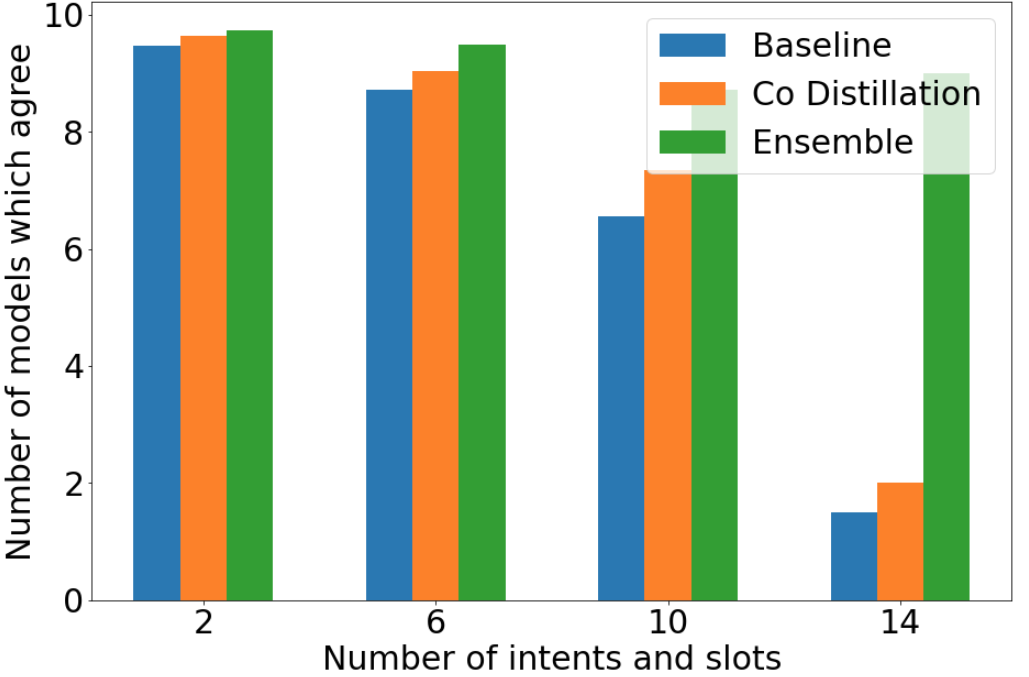
We also explore the relation between agreement and the length of the structured output sequences. Figure 2 plots the number of models in agreement against the number of intents and slots. In making a structured prediction during inference, as length increases the model has more freedom to select incorrect tokens and therefore churn increases. Co-distillation increases agreement for longer sequences, but ensembling is especially robust. Table 7 reports the average target and prediction length where all models disagree. Surprisingly, we observe that the models over-generate compared to the target; however, the difference is reduced with co-distillation/ensembling.
| Method | Target | Prediction |
|---|---|---|
| Baseline | 3.66 | 3.91 |
| Co-distillation | 3.77 | 3.82 |
| 4 layer ensemble | 3.56 | 3.70 |
Practical considerations
We roughly compare the methods along the resource usage dimension in Table 8. As resource usage may be implementation or architecture dependent, we report the number of parameters, which correlates strongly with training/inference time and memory. While ensembling is the strongest approach, it also comes with the most expensive inference. Although wall-clock inference time may be the same as the base model due to parallelization, computing power and memory scales by a factor of . Further, while distillation methods have the same inference time due to similar sized outputs, they have different costs w.r.t. training the teacher.88 8 Hard/soft distillation have equal number of parameters. For ensemble distillation, the teacher models can be trained in parallel, but still have storage requirements. For large-model distillation, in practice our 12-layer teacher has about times the number of parameters as the baseline. In both cases, the student must be trained sequentially. Overall, co-distillation performs consistently well across different datasets and noise settings in terms of EM and model agreement while striking a balance between computational cost and performance, rendering it an attractive approach for goal-oriented conversational semantic parsing.
| Method | Training (actual) | Inference (actual) |
|---|---|---|
| Baseline | ||
| Ensemble | ||
| Ens. distillation | ||
| Large distillation | ||
| Co-distillation |
8 Conclusion
Our experiments showed that there exists substantial churn across runs when re-training models on the same conversational semantic parsing datasets. We showed that for “production-sized” models, co-distillation with label smoothing increases agreement without loss of accuracy. Furthermore, on noisy data simulating a real-world environment, the improvement is even more drastic. When we account for resource usage along with accuracy, we provide strong evidence that co-distillation provides the sweet spot compared to methods like hard/soft distillation and ensembling.
In future work, we plan to explore how other modeling decisions can increase or decrease model churn. In this work, we limited our focus to BERT encoders with different number of layers. Other questions to explore include whether the choice of pre-training technique affects churn or whether pre-trained encoder-decoders show the same effects. Finally, we will examine whether alternative decoding algorithms, such as non-autoregressive approaches Babu et al. 2021; Oh et al. 2022, can reduce churn.
References
- Aghajanyan et al. (2020) Armen Aghajanyan, Jean Maillard, Akshat Shrivastava, Keith Diedrick, Michael Haeger, Haoran Li, Yashar Mehdad, Veselin Stoyanov, Anuj Kumar, Mike Lewis, and Sonal Gupta. 2020. Conversational semantic parsing. In Proceedings of the 2020 Conference on Empirical Methods in Natural Language Processing (EMNLP), pages 5026–5035, Online. Association for Computational Linguistics.
- Anil et al. (2018) Rohan Anil, Gabriel Pereyra, Alexandre Passos, Robert Ormandi, George E. Dahl, and Geoffrey E. Hinton. 2018. Large scale distributed neural network training through online distillation. In International Conference on Learning Representations.
- Babu et al. (2021) Arun Babu, Akshat Shrivastava, Armen Aghajanyan, Ahmed Aly, Angela Fan, and Marjan Ghazvininejad. 2021. Non-autoregressive semantic parsing for compositional task-oriented dialog. In Proceedings of the 2021 Conference of the North American Chapter of the Association for Computational Linguistics: Human Language Technologies, pages 2969–2978, Online. Association for Computational Linguistics.
- Bahri and Jiang (2021) Dara Bahri and Heinrich Jiang. 2021. Locally adaptive label smoothing improves predictive churn. In Proceedings of the 38th International Conference on Machine Learning, volume 139 of Proceedings of Machine Learning Research, pages 532–542. PMLR.
- Chen et al. (2020a) Xilun Chen, Asish Ghoshal, Yashar Mehdad, Luke Zettlemoyer, and Sonal Gupta. 2020a. Low-resource domain adaptation for compositional task-oriented semantic parsing. In Proceedings of the 2020 Conference on Empirical Methods in Natural Language Processing (EMNLP), pages 5090–5100, Online. Association for Computational Linguistics.
- Chen et al. (2020b) Yen-Chun Chen, Zhe Gan, Yu Cheng, Jingzhou Liu, and Jingjing Liu. 2020b. Distilling knowledge learned in BERT for text generation. In Proceedings of the 58th Annual Meeting of the Association for Computational Linguistics, pages 7893–7905, Online. Association for Computational Linguistics.
- Cheng et al. (2020) Jianpeng Cheng, Devang Agrawal, Héctor Martínez Alonso, Shruti Bhargava, Joris Driesen, Federico Flego, Dain Kaplan, Dimitri Kartsaklis, Lin Li, Dhivya Piraviperumal, Jason D. Williams, Hong Yu, Diarmuid Ó Séaghdha, and Anders Johannsen. 2020. Conversational semantic parsing for dialog state tracking. In Proceedings of the 2020 Conference on Empirical Methods in Natural Language Processing (EMNLP), pages 8107–8117, Online. Association for Computational Linguistics.
- Coucke et al. (2018) Alice Coucke, Alaa Saade, Adrien Ball, Théodore Bluche, Alexandre Caulier, David Leroy, Clément Doumouro, Thibault Gisselbrecht, Francesco Caltagirone, Thibaut Lavril, Maël Primet, and Joseph Dureau. 2018. Snips voice platform: an embedded spoken language understanding system for private-by-design voice interfaces. CoRR, abs/1805.10190.
- Damonte et al. (2019) Marco Damonte, Rahul Goel, and Tagyoung Chung. 2019. Practical semantic parsing for spoken language understanding. In Proceedings of the 2019 Conference of the North American Chapter of the Association for Computational Linguistics: Human Language Technologies, Volume 2 (Industry Papers), pages 16–23, Minneapolis, Minnesota. Association for Computational Linguistics.
- D’Amour et al. (2020) Alexander D’Amour, Katherine A. Heller, Dan Moldovan, Ben Adlam, Babak Alipanahi, Alex Beutel, Christina Chen, Jonathan Deaton, Jacob Eisenstein, et al. 2020. Underspecification presents challenges for credibility in modern machine learning. CoRR, abs/2011.03395.
- Devlin et al. (2019) Jacob Devlin, Ming-Wei Chang, Kenton Lee, and Kristina Toutanova. 2019. BERT: Pre-training of deep bidirectional transformers for language understanding. In Proceedings of the 2019 Conference of the North American Chapter of the Association for Computational Linguistics: Human Language Technologies, Volume 1 (Long and Short Papers), pages 4171–4186, Minneapolis, Minnesota. Association for Computational Linguistics.
- Dietterich (2000) Thomas G. Dietterich. 2000. Ensemble methods in machine learning. In MULTIPLE CLASSIFIER SYSTEMS, LBCS-1857, pages 1–15. Springer.
- Dodge et al. (2019) Jesse Dodge, Suchin Gururangan, Dallas Card, Roy Schwartz, and Noah A. Smith. 2019. Show your work: Improved reporting of experimental results. In Proceedings of the 2019 Conference on Empirical Methods in Natural Language Processing and the 9th International Joint Conference on Natural Language Processing (EMNLP-IJCNLP), pages 2185–2194, Hong Kong, China. Association for Computational Linguistics.
- Dodge et al. (2020) Jesse Dodge, Gabriel Ilharco, Roy Schwartz, Ali Farhadi, Hannaneh Hajishirzi, and Noah A. Smith. 2020. Fine-tuning pretrained language models: Weight initializations, data orders, and early stopping. CoRR, abs/2002.06305.
- Golovin et al. (2017) Daniel Golovin, Benjamin Solnik, Subhodeep Moitra, Greg Kochanski, John Elliot Karro, and D. Sculley, editors. 2017. Google Vizier: A Service for Black-Box Optimization.
- Guo et al. (2017) Chuan Guo, Geoff Pleiss, Yu Sun, and Kilian Q. Weinberger. 2017. On calibration of modern neural networks. In ICML, pages 1321–1330.
- Gupta et al. (2018) Sonal Gupta, Rushin Shah, Mrinal Mohit, Anuj Kumar, and Mike Lewis. 2018. Semantic parsing for task oriented dialog using hierarchical representations. In Proceedings of the 2018 Conference on Empirical Methods in Natural Language Processing, pages 2787–2792, Brussels, Belgium. Association for Computational Linguistics.
- Hansen and Salamon (1990) L. K. Hansen and P. Salamon. 1990. Neural network ensembles. IEEE Trans. Pattern Anal. Mach. Intell., 12(10):993–1001.
- Hinton et al. (2015) Geoffrey Hinton, Oriol Vinyals, and Jeffrey Dean. 2015. Distilling the knowledge in a neural network. In NIPS Deep Learning and Representation Learning Workshop.
- Jiang et al. (2022) Heinrich Jiang, Harikrishna Narasimhan, Dara Bahri, Andrew Cotter, and Afshin Rostamizadeh. 2022. Churn reduction via distillation. In International Conference on Learning Representations.
- Kim and Rush (2016) Yoon Kim and Alexander M. Rush. 2016. Sequence-level knowledge distillation. In Proceedings of the 2016 Conference on Empirical Methods in Natural Language Processing, pages 1317–1327, Austin, Texas. Association for Computational Linguistics.
- Lakshminarayanan et al. (2017) Balaji Lakshminarayanan, Alexander Pritzel, and Charles Blundell. 2017. Simple and scalable predictive uncertainty estimation using deep ensembles. In Advances in Neural Information Processing Systems, volume 30. Curran Associates, Inc.
- Li et al. (2021) Haoran Li, Abhinav Arora, Shuohui Chen, Anchit Gupta, Sonal Gupta, and Yashar Mehdad. 2021. MTOP: A comprehensive multilingual task-oriented semantic parsing benchmark. In Proceedings of the 16th Conference of the European Chapter of the Association for Computational Linguistics: Main Volume, pages 2950–2962, Online. Association for Computational Linguistics.
- Lialin et al. (2020) Vladislav Lialin, Rahul Goel, Andrey Simanovsky, Anna Rumshisky, and Rushin Shah. 2020. Continual learning for neural semantic parsing. CoRR, abs/2010.07865.
- Loshchilov and Hutter (2017) Ilya Loshchilov and Frank Hutter. 2017. Fixing weight decay regularization in adam. CoRR, abs/1711.05101.
- McCoy et al. (2020) R. Thomas McCoy, Junghyun Min, and Tal Linzen. 2020. BERTs of a feather do not generalize together: Large variability in generalization across models with similar test set performance. In Proceedings of the Third BlackboxNLP Workshop on Analyzing and Interpreting Neural Networks for NLP, pages 217–227, Online. Association for Computational Linguistics.
- Milani Fard et al. (2016) Mahdi Milani Fard, Quentin Cormier, Kevin Canini, and Maya Gupta. 2016. Launch and iterate: Reducing prediction churn. In Advances in Neural Information Processing Systems, volume 29. Curran Associates, Inc.
- Mosbach et al. (2021) Marius Mosbach, Maksym Andriushchenko, and Dietrich Klakow. 2021. On the stability of fine-tuning {bert}: Misconceptions, explanations, and strong baselines. In International Conference on Learning Representations.
- Müller et al. (2019) Rafael Müller, Simon Kornblith, and Geoffrey E Hinton. 2019. When does label smoothing help? In Advances in Neural Information Processing Systems, volume 32. Curran Associates, Inc.
- Nie et al. (2020) Yixin Nie, Xiang Zhou, and Mohit Bansal. 2020. What can we learn from collective human opinions on natural language inference data? In Proceedings of the 2020 Conference on Empirical Methods in Natural Language Processing (EMNLP), pages 9131–9143, Online. Association for Computational Linguistics.
- Oh et al. (2022) Geunseob Oh, Rahul Goel, Christopher Hidey, Shachi Paul, Aditya Gupta, Pararth Shah, and Rushin Shah. 2022. Improving top-k decoding for non-autoregressive semantic parsing via intent conditioning. CoRR, abs/2204.06748.
- Reich et al. (2020) Steven Reich, David Mueller, and Nicholas Andrews. 2020. Ensemble Distillation for Structured Prediction: Calibrated, Accurate, Fast—Choose Three. In Proceedings of the 2020 Conference on Empirical Methods in Natural Language Processing (EMNLP), pages 5583–5595, Online. Association for Computational Linguistics.
- Rongali et al. (2020) Subendhu Rongali, Luca Soldaini, Emilio Monti, and Wael Hamza. 2020. Don’t Parse, Generate! A Sequence to Sequence Architecture for Task-Oriented Semantic Parsing, page 2962–2968. Association for Computing Machinery, New York, NY, USA.
- Shamir and Coviello (2020) Gil I. Shamir and Lorenzo Coviello. 2020. Anti-distillation: Improving reproducibility of deep networks. CoRR, abs/2010.09923.
- Shamir et al. (2020) Gil I. Shamir, Dong Lin, and Lorenzo Coviello. 2020. Smooth activations and reproducibility in deep networks. CoRR, abs/2010.09931.
- Szegedy et al. (2016) Christian Szegedy, Vincent Vanhoucke, Sergey Ioffe, Jon Shlens, and Zbigniew Wojna. 2016. Rethinking the inception architecture for computer vision. In 2016 IEEE Conference on Computer Vision and Pattern Recognition (CVPR), pages 2818–2826.
- Turc et al. (2019) Iulia Turc, Ming-Wei Chang, Kenton Lee, and Kristina Toutanova. 2019. Well-read students learn better: The impact of student initialization on knowledge distillation. CoRR, abs/1908.08962.
- Vaswani et al. (2017) Ashish Vaswani, Noam Shazeer, Niki Parmar, Jakob Uszkoreit, Llion Jones, Aidan N Gomez, Ł ukasz Kaiser, and Illia Polosukhin. 2017. Attention is all you need. In Advances in Neural Information Processing Systems, volume 30. Curran Associates, Inc.
- Williams and Zipser (1989) Ronald J. Williams and David Zipser. 1989. A Learning Algorithm for Continually Running Fully Recurrent Neural Networks. Neural Computation, 1(2):270–280.
Appendix A Ethics
The TOP and SNIPS datasets used in this experiments are intended for research purposes only. We verified that the datasets do not contain personally identifiable information. The risks of dual use for task-oriented conversational semantic parsers are low as we are not performing open-ended generation; however, the models are likely to overfit to certain demographic groups and underperform on others.
Appendix B Hyper-parameter Search and Settings
We run our experiments on the TPU v2 available through Google Cloud.99 9 https://cloud.google.com/tpu
We use the same hyper-parameters for all 3 TOP datasets and SNIPS, except for SNIPS we use a different number of training steps and learning rate. The hyper-parameters were selected using the Google Cloud black box optimizer Golovin et al. 2017. We tuned the parameters using 64 re-runs over the settings described in Table 9. For SNIPS, we held out 10% of the training data for tuning the training steps (100000) and learning rate () and trained the final models on 100% of the training data with the selected hyper-parameters. For distillation experiments we adjusted the learning rate to and the batch size to 128 to prevent overfitting.
We train all models (including teacher and student) for 300000 steps on the TOP datasets and 100000 on SNIPS. We use the Adam optimizer with weight decay Loshchilov and Hutter 2017 and the relu activation function. To follow the pointer generator approach of Rongali et al. 2020, we embed the output vocabulary in 128-dimensional vectors and project the BERT embeddings from the input to 128 dimensions as well. For our transformer decoder Vaswani et al. 2017, we use 2 heads and 2 layers (see Table 9) with 256 dimensions for the attention and feed forward layers. We also use a maximum output length of 51. We use dropout on the input wordpiece embeddings, after the contextual BERT embeddings, and on the output embeddings before the softmax layer.
| Hyper-parameter | Range/Set | Selected Value |
|---|---|---|
| Learning rate | 4e-5 | |
| Decoder Heads | 2 | |
| Decoder Layers | 4 | |
| Batch Size | 256 | |
| Dropout | 0.0316 |
Appendix C Additional Examples
| Query | Ground Truth | Model predictions | |
| play new matchbox 20 | [in:play_music [sl:music_artist_name matchbox 20 ]] | [in:play_music [sl:music_track_title matchbox 20 ]] | |
| [in:play_music [sl:music_artist_name matchbox 20 ]] | |||
| repeat closer | [in:replay_music [sl:music_track_title closer ]] | [in:replay_music [sl:music_track_title closer ]] | |
| [in:loop_music ] | |||
| Churn examples fixed by co-distillation. Model predictions are from the baseline model | |||
| show me alarms for tomorrow | [in:get_alarm [sl:date_time for tomorrow ]] | [in:get_alarm [sl:alarm_name [in:get_time [sl:date_time for tomorrow ]]]] | |
| [in:get_alarm [sl:date_time for tomorrow ]] | |||
| take out my wednesday alarm. | [in:delete_alarm [sl:alarm_name | [in:delete_alarm [sl:alarm_name [in:get_time [sl:date_time wednesday ]]]] | |
| [in:get_time [sl:date_time wednesday ]]]] | [in:silence_alarm [sl:alarm_name [in:get_time [sl:date_time wednesday ]]]] | ||
| Churn examples further fixed by ensembling. Model predictions from the co-distilled model | |||
Appendix D Additional Results
We present the full set of results from Table 5 in Table 11. The results in Table 11(a) provide strong evidence that co-distillation with label smoothing (Table 11(b)) is clearly preferable. When we examine the full set of datasets and methods combined with label smoothing in the random/systematic noise setting, we also see that soft distillation from an ensemble performs well. However, in some cases soft ensemble distillation performs worse than the baseline; swapping occasionally slightly better performance for occasionally much worse performance would not be an acceptable tradeoff in most cases. Co-distillation is more stable in terms of consistently outperforming the baseline. Furthermore, co-distillation requires fewer resources and can be trained in parallel.
| TOP | TOPv2 | MTOP | SNIPS | |||||
| Model | EM (@10) | AGR | EM (@10) | AGR | EM (@10) | AGR | EM (@10) | AGR |
| BERT-4 | 81.51 (72.14) | 77.85 | 83.74 (73.18) | 78.47 | 80.13 (68.71) | 72.54 | 86.83 (75.25) | 78.42 |
| Ensemble | 84.60 (78.55) | 86.18 | 86.42 (80.38) | 88.17 | 84.59 (78.52) | 84.39 | 87.69 (80.58) | 84.60 |
| SD (ensemble) | 81.36 (71.63) | 77.25 | 83.73 (72.62) | 77.72 | 79.50 (68.11) | 71.97 | 86.80 (75.11) | 77.84 |
| SD (BERT-12) | 81.31 (71.16) | 76.43 | 83.51 (72.13) | 77.10 | 79.87 (67.36) | 70.76 | 86.37 (73.96) | 76.69 |
| HD (BERT-12) | 81.33 (70.91) | 75.92 | 83.56 (72.15) | 76.99 | 79.66 (67.09) | 70.39 | 86.93 (77.12) | 80.29 |
| Co-distillation | 81.31 (72.04) | 77.98 | 84.01 (73.96) | 79.49 | 79.55 (68.48) | 72.95 | 87.39 (79.28) | 82.59 |
| TOP | TOPv2 | MTOP | SNIPS | |||||
| Model | EM (@10) | AGR | EM (@10) | AGR | EM (@10) | AGR | EM (@10) | AGR |
| BERT-4 | 77.90 (64.28) | 68.76 | 82.39 (71.11) | 76.24 | 70.01 (44.97) | 46.63 | 76.59 (51.08) | 52.95 |
| Ensemble | 78.67 (72.21) | 80.55 | 83.78 (76.53) | 83.89 | 72.37 (58.78) | 65.24 | 82.27 (67.23) | 70.50 |
| SD (ensemble) | 80.14 (70.59) | 76.45 | 83.51 (74.31) | 80.46 | 71.14 (48.89) | 51.27 | 80.96 (61.01) | 63.17 |
| SD (BERT-12) | 78.71 (66.96) | 72.05 | 82.71 (70.75) | 75.50 | 69.83 (45.26) | 47.09 | 78.59 (53.09) | 55.54 |
| HD (BERT-12) | 77.71 (64.77) | 69.54 | 81.11 (60.39) | 63.08 | 69.63 (44.78) | 46.52 | 76.70 (47.34) | 48.92 |
| Co-distillation | 78.91 (68.42) | 74.54 | 82.60 (73.07) | 79.34 | 73.74 (57.64) | 61.22 | 82.50 (68.35) | 71.80 |
| TOP | TOPv2 | MTOP | SNIPS | |||||
| Model | EM (@10) | AGR | EM (@10) | AGR | EM (@10) | AGR | EM (@10) | AGR |
| BERT-4 | 79.66 (65.28) | 70.17 | 83.03 (72.27) | 77.74 | 74.58 (58.50) | 62.86 | 84.19 (68.20) | 70.94 |
| Ensemble | 79.87 (68.78) | 74.52 | 83.40 (73.60) | 79.75 | 77.59 (68.55) | 75.80 | 84.50 (71.22) | 74.53 |
| SD (ensemble) | 81.02 (71.71) | 77.87 | 83.85 (74.46) | 80.68 | 74.97 (58.87) | 63.30 | 82.24 (57.12) | 59.14 |
| SD (BERT-12) | 80.75 (71.22) | 77.15 | 83.25 (73.19) | 78.97 | 75.01 (59.28) | 63.30 | 82.59 (63.02) | 65.90 |
| HD (BERT-12) | 79.49 (64.51) | 69.10 | 82.93 (72.27) | 77.94 | 75.21 (57.11) | 60.51 | 81.57 (59.71) | 62.88 |
| Co-distillation | 80.84 (73.61) | 81.27 | 83.19 (73.96) | 80.50 | 76.98 (63.64) | 68.09 | 85.49 (72.09) | 76.26 |