Active Learning with Label Comparisons
Abstract
Supervised learning typically relies on manual annotation of the true labels. When there are many potential classes, searching for the best one can be prohibitive for a human annotator. On the other hand, comparing two candidate labels is often much easier. We focus on this type of pairwise supervision and ask how it can be used effectively in learning, and in particular in active learning. We obtain several insightful results in this context. In principle, finding the best of labels can be done with active queries. We show that there is a natural class where this approach is sub-optimal, and that there is a more comparison-efficient active learning scheme. A key element in our analysis is the “label neighborhood graph” of the true distribution, which has an edge between two classes if they share a decision boundary. We also show that in the PAC setting, pairwise comparisons cannot provide improved sample complexity in the worst case. We complement our theoretical results with experiments, clearly demonstrating the effect of the neighborhood graph on sample complexity.
1 Introduction
Supervised learning is a central paradigm in the empirical success of machine learning in general, and deep learning in particular. Despite the recent advances in unsupervised learning, and in particular self-training, large amounts of annotated data are still required in order to achieve high accuracy in many tasks. The main difficulty with supervised learning is, of course, the manual effort needed for annotating examples. Annotation becomes particularly challenging when there are many classes to consider. For example, in a text summarization task, we can ask an annotator to write a summary of the source text, but this will likely not result in the “best” summary. We could also present the annotator a summary and ask for feedback (e.g. is it good), but the quality could be difficult to judge in isolation. We could also ask the annotator to select the best summary out of a set of candidates (e.g. produced by a language model), but this could be taxing if not infeasible when there are many candidates.
Motivated by the above scenario, previous works [e.g., see Stiennon et al. 2020, Ouyang et al. 2022, for a recent application to large language models] have considered an alternative, and arguably natural, form of supervision: “Label Comparisons”. Instead of presenting many potential labels to the annotator (e.g., candidate text summaries), we only present two candidates and ask the annotator to choose the better one. For example, when summarizing Snow White, we can ask to compare the summaries “A story about an evil step-mother” and “A story about a girl who is driven to the forest by an evil step-mother and ends up living with dwarves”. Most annotators would easily choose the latter as a better summary.
Label comparisons clearly require a much lighter cognitive load than considering all alternatives, and thus have high potential as an annotation mechanism. However, our theoretical understanding of this mechanism is fairly limited. While there has been work on learning to rank, which also uses comparisons, the goal of label comparisons is typically not to learn a complete ranking, but rather to build a model that outputs optimal predictions. Here we set out to analyze label comparisons from this perspective, and we obtain several surprising results and a new algorithm.
Our key question is what is the best way to learn with label comparisons. We assume that during learning we can only ask an annotator for label comparisons and not, for example, for the ground-truth label of the input, which we refer to as an argmax query. We then ask how one can design algorithms that make effective use of such queries, and what is the corresponding query complexity. Namely, how many queries are needed to achieve a given test error. Perhaps the most natural way of using comparisons is simply for finding the argmax label, which can be done via active queries. However, as we shall see, this is a suboptimal approach.
The first question we ask is whether access to comparisons is more informative than access to the argmax. If we know all comparisons for , we can also infer the argmax and so it would seem like the answer to this should be in the affirmative. Our first result shows that in the PAC setting, this is in fact not the case, and that knowing all comparisons may result in the same sample complexity as knowing only the argmax. The intuition for this negative result is that for 1D classifiers, the informative points are those that lie close to the decision boundaries between classes, and the argmax label for these points can also be used to find the boundaries, so that comparisons do not provide further advantage.
The negative result above may seem to suggest that comparisons are only useful for inferring the argmax. However, we show that in the case of active learning, comparisons can be used more effectively. We consider the setting where the active learner can choose which label comparison queries to request for a given input (including not requesting any queries at all). A natural approach here is to take a “standard” active learning algorithm based on argmax queries, and implement it using pairwise comparisons, by using active comparisons for each input to obtain the argmax. This strategy results in an algorithm that asks comparisons, where is the number of argmax queries used.
Here we show that one can in fact do better than simulating argmax, by asking the “right” comparisons in an active fashion. These beneficial comparisons are closely related to the “Label Neighborhood Graph” (see Figure 2) where labels are neighbors if they share a decision boundary. We show that it is sufficient to ask queries only about neighbor pairs in this graph. Thus, if this graph is sparse, active learning can be implemented with fewer queries. In particular, for linear classifiers in , each class has at most two neighbors, and thus the neighborhood graph is very sparse, and our proposed active learning approach is highly effective. Taken together, our results demonstrate the richness of the label-comparison setting, and the ways in which its query complexity depends on the structure of the data.
2 Related Work
Several lines of works have addressed alternative modes of supervision for multi-class learning.
Bandit Feedback: In this setting (e.g., Kakade et al. 2008, Crammer and Gentile 2013) the learner only observes whether its predicted class is correct or not. On the one hand, this feedback is stronger than label comparisons, because positive bandit feedback implies knowledge of the argmax. On the other hand, label comparisons provide more information than bandit feedback, because comparisons provide knowledge about relative ordering of non-argmax labels.
Maxing from pairwise comparisons. Maximum selection (maxing) from noisy comparisons is well-studied problem. Falahatgar et al. 2018 give an overview of known results under various noise models. Here, we show that for multiclass learning, using comparisons to first learn the global structure of the problem is more efficient than only using them for maxing. Daskalakis et al. 2011 consider maxing in partially ordered sets, where some pairs may be incomparable, which is interesting to explore in our setting.
Dueling Bandits: In online learning, learning from pairwise comparisons is studied under the dueling bandits setting [Saha et al. 2021, Dudík et al. 2015], in which the learner “pulls” a pair of arms and observes the result of a noisy comparison (duel) between them. The objective in these cases is to minimize the regret w.r.t a solution-concept from the social choice literature, such as the Condorcet winner [Yue et al. 2012], Borda winner, Copeland winner, or the Von Neuman winner [Dudík et al. 2015]. The focus on such regret minimization objectives is principally different from ours, since our primary goal is to minimize the number of queries made, rather than minimizing an online loss.
Active Learning with rich supervision: Several works have explored alternative forms of supervision. Balcan and Hanneke 2012 explore class-conditional queries, where the annotator is given a target label and a pool of examples, and must say whether one of the examples matches the target label. Several works [Kane et al. 2017, Hopkins et al. 2020, Xu et al. 2017] have studied comparison queries on instances, where the annotator receives two inputs and reports which one is more positive (for binary classification). Ben-Eliezer et al. 2022 study active learning of polynomial threshold functions in using derivative queries (e.g., is a patient getting sicker or healthier?). Our supervision is conceptually different from all of these, as it compares between several labels on the same example .
Learning Ranking as a Reward Signal: A recent line of work demonstrated that pairwise label-comparisons elicited from humans can be used to improve the performance of LLMs. Stiennon et al. 2020 collect a dataset of human comparisons between summaries of a given text, and use it to obtain better summarization policies, and Ouyang et al. 2022 extend this idea to aligning LLMs with user intent. Our focus here is to understand the theoretical properties of such label comparisons, which we expect will result in more effective ways of collecting and using such comparisons.
3 Preliminaries
Multi-class learning. Let denote the feature space and denote the label space, consisting of classes. We use to denote an (unknown) distribution on and to denote a class of target functions, . In this work, our focus is on a realizable setting in which the target function is some (unknown) . For and a class , is the score assigned to class on instance . Given a target function , the loss of a candidate classifier is the standard (multiclass) 0-1 loss: .
Since we are interested in how the difficulty of learning scales with the number of classes , we will explicitly parameterize hypothesis classes in terms of , . For example, the class of homogeneous linear classifiers11 1 Our convention will be to use homogeneous linear classifiers. Thus when we refer to our results for 1d, we mean the class . over classes in dimension is , where .
Supervision Oracles. Pertinent to this work is a distinction between two types of access to the target multiclass function: argmax (i.e. label) queries and label-comparison queries.
Definition 3.1 (Supervision Oracles).
Given a target function , we define the following oracles:
In the rest of the manuscript we simply use to denote the supervision oracle, where it’s understood that if it receives an input it invokes the argmax oracle and if it receives a triplet it invokes the comparisons oracle.
4 Passive learning
We define the sample and query complexities of PAC learnability using both argmax and label-comparisons supervision.22 2 For simplicity, we consider a PAC notion where the goal is to return -accurate solutions with constant probability (e.g. 14/15). We begin with the usual passive learning setup, and differentiate between the situation in which every example arrives with its argmax (i.e., the standard PAC setup), and where every example arrives with all the pairwise label comparisons (essentially, the total order on the classes).
Definition 4.1 (Sample complexity of passive learning with argmax supervision).
Fix a distribution over and a target function . Let denote the distribution on in which a sample is generated by drawing and taking .
We say that the sample complexity of passively learning a class is if there exists a learning algorithm with the following property: for every distribution on , for every , for every , and for every , given i.i.d samples from , the algorithm returns an hypothesis s.t w.p at least , .
Definition 4.2 (Sample complexity of passive learning with label-comparisons.).
Fix a distribution over and a target function . Let denote a distribution on where a sample is generated by drawing and for , taking . We say that the sample complexity of passively learning a class is if there exists a learning algorithm with the following property: for every distribution on , for every , for every , and for every , given i.i.d samples from , the algorithm returns an hypothesis s.t w.p at least , .
Note that in the latter setting, the learner receives strictly more information about every example than in the argmax supervision setting. Namely, the argmax can always be inferred from the total order on the classes. We will therefore consider label-comparisons as helpful in this setup if knowing all comparisons results in improvement to the sample complexity. Our first result is negative: in general, label-comparisons may not be helpful in the passive regime.

Theorem 4.3.
Any algorithm that PAC learns must use samples, irrespective of whether it has access to argmax or label-comparison supervision.
Proof.
For regular PAC learning (with argmax supervision), the standard approach for lower bounding the sample complexity is to lower bound the Natarajan dimension [Natarajan 1989]. To extend this result to the setting of Definition 4.2, we employ a suitable variant of the dimension introduced in Daniely and Shalev-Shwartz 2014. Following Brukhim et al. 2022, we refer to it as the Daniely-Shwartz dimension. It provides a tighter lower bound on the sample complexity, and it is also easier to adapt to our label comparison setting.
To emphasize the difference between functions mapping to a single class and functions mapping to a total order over the classes, we will denote the former with and the latter with (and likewise for hypotheses classes). We write for the class ranked first in the total order .
Definition 4.4.
Given a set , we say that and are -close if:
With this we can define a variant of Definition 12 in Daniely and Shalev-Shwartz 2014 for the case of extra supervision.
Definition 4.5 (The Daniely-Shwartz dimension for label comparisons.).
A set is shattered by if there exists a finite subset of functions with the following property: for every and for every , there exists such that are -close. The Daniely-Shwartz dimension of , , is the maximal cardinality of a shattered set.
In Appendix A, we prove that the sample complexity of passively learning a class with label-comparisons (Definition 4.2) is . Thus, our objective is to prove that .
To show this, we will construct a shattered set of size for . Consider labels of the form , where and . Partition the numbers to triples: , , . We claim that middle points, are shattered by . Showing this requires defining a subset of with the property of Definition 4.5. To define each function we will use an equivalent parametrization of linear classifiers in 1d as 1NN classification. i.e., each total order in is parameterized by , where the total order is the one implied by sorting the classes according to the distance of their centers to . See Figure 1 for an illustration. With this parameterization in mind, consists of all functions which satisfy the following: for each , the centers corresponding to labels and are located in the ’th triplet, and exactly one of them is located in the middle of the triplet, on the point . By construction, (for each of the triplets we need to specify which of the two centers is located in the middle of the triplet, and whether to locate the other center on the left or on the right of it).
To see that is shattered, consider and a point . W.l.o.g, assume that the center located on is . We define based on the location of the center of , which by definition of , could be either to the right (on ) or to the left (on ). In the first case, is obtained by shifting both centers one unit to the left: in the center is located on and the center is located on . In the second case, is obtained by shifting both centers one unit to the right: in the center is located on and the center is located on . By the definition of , . Crucially, and are -close (Definition 4.4): moving from to the center located on (and therefore the argmax) has changed, but the total order for every other point in is remained unchanged, per the requirement of Definition 4.4. This proves is shattered, and so , as required. ∎
Remark. An interesting open question is whether this negative result can be extended to other classes (e.g. linear classifiers in higher dimensions). Technically, this requires lower bounding the the DS dimension of the class, as we did here for . We conjecture that for the negative result can be extended in a distribution-specific manner (e.g., restricting to distributions with properties such as margin and sparsity); see the discussion in Appendix B, where we report experimental results for the passive learning setting.
5 Active Learning
Next, we consider the active learning setting. Specifically, we focus on pool-based active learning, where the learner has access to unlabeled samples and can decide which queries to ask the oracle for (including not asking any queries). The performance of the algorithm is now measured in terms of the query complexity, namely the number of queries it makes to the labeling oracle in question.
Definition 5.1 (Query complexity of active learning.).
The query complexity of actively learning a class is if there exists a function and a learning algorithm with the following property: for every distribution on , for every , for every , and for every , given i.i.d samples from and at most queries to , the algorithm returns an hypothesis s.t w.p at least , . We refer to as the query complexity of learning with argmax supervision or with label-comparison supervision, depending the oracle .
We note that every active learning algorithm that uses argmax queries can always be simulated using comparison queries: in the adaptive setting (where the choice of query to ask at time can depend on the previous answers), label-comparison queries suffice to implement a “tournament” that reveals the argmax. This provides a generic way to use the label-comparison oracle: simply request the label-comparison queries necessary for a “regular” active learner. We therefore say that comparisons are useful for active learning if the number of label-comparison queries required to learn a class is strictly lower than the number of label-comparison queries required to simulate the best active learner that uses argmax queries to learn .
Interestingly, the distinction between passive and active learning is important. Our main result is that when the learner is allowed to decide which queries to request, label-comparisons are helpful: we provide a learning algorithm that uses label comparisons more efficiently than simply using them to implement the best “regular” active learner.
Theorem 5.2.
The label-comparison query complexity for active learning is , whereas the query complexity of simulating the best argmax active learner is .
The proof of Theorem 5.2 will employ a specific multiclass to binary reduction that uses the concept of the label neighborhood graph of the target classifier. Intuitively, two classes and are considered neighboring if they share a decision boundary; i.e., there are two arbitrarily close points in , where for one the argmax is and for the other the argmax is . See Figure 2 for an example of the label neighborhood graph of a linear classifier in .
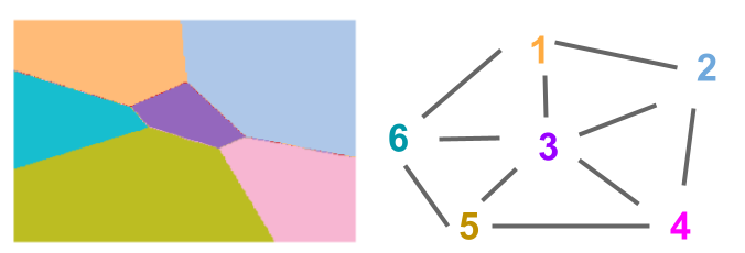
Definition 5.3 (Label Neighborhood graph).
Fix a continuous function . The neighborhood graph is an undirected graph on vertices, with an edge between vertices and if and only if there exists for which for every , .
To simplify notation, we use to refer to an edge in , and for the total number of edges. The degree of is the number of neighbors has in .
We next define (Neighborhood Graph Multiclass-to-Binary), a procedure for actively learning a multiclass classifier using a neighborhood graph (see Algorithm 1). Given as input a binary active learning algorithm and a neighborhood graph, it uses comparison queries to learn a binary classifier for distinguishing every pair of neighboring classes in . It then aggregates these into a multi-class classifier using the following scheme:
Definition 5.4 (Binary to multiclass aggregation.).
Fix , where is a neighborhood graph and is a collection of binary classifiers, one for every edge in . The graph-based aggregation of is a function defined as follows:
Namely, the label of is the class in that won the largest fraction of “duels” against its neighbors in the graph .
An important component in analyzing is the following lemma. It establishes that when invoked w.r.t the true neighborhood graph , if the binary classifiers are sufficiently accurate, then so is the resulting multiclass classifier. See Supplementary E for proof.
Lemma 5.5.
Fix a distribution on and a classifier . Fix . If and every has error at most , then has error at most .
From this, we obtain the following upper bound on the query complexity of learning using label comparisons.
Corollary 5.6.
If the target neighborhood graph is known, the label-comparison query complexity of learning is , where is the query complexity of active learning in the binary case (i.e. ).
Corollary 5.6 suggests that label-comparisons will be useful when (i) the target neighborhood graph is sparse (has low degree), and (ii) it can be learned with relatively few label-comparisons. We are now ready to prove Theorem 5.2: we will show that for learning (the class for which we demonstrated comparisons are not useful in the passive setting), both these conditions hold. Hence, comparisons indeed provide a provable gain over argmax supervision.
Proof of Theorem 5.2: We will begin by instantiating the bound from Corollary 5.6 for . Consider the degree of the neighborhood graph. Using the equivalent parameterization of linear classifiers in (see Figure 1), it follows that every class has at most neighbors: exactly the preceding and succeeding classes in the sorted order of the classes. Thus, for every , . Second, active learning in is well-understood: unlike higher dimensions, the distribution-free query complexity of active learning for two classes is using binary search over [Dasgupta 2004]. Plugging both of these facts into the upper bound of Corollary 5.6, we conclude that the query complexity for learning when the target neighborhod graph is known is .
Next, we turn to the question of learning using label-comparison queries. Towards this, consider Algorithm 2. The algorithm receives a sample of points from and uses exactly label comparisons to return a neighborhood graph . As we claim below the graph will be identical to , except for possibly a set of edges pertaining to classes outside whose overall probability under is smaller than . The key observation behind Algorithm 2 is that we can use exactly two label-comparison queries to infer whether a class appears before a class , as long as both classes are “represented” in .33 3 We say a class is represented in if the position of in the total order of all the classes is greater-equal than the position of and smaller-equal than the position of . We can therefore use a total of queries to infer the total order of all the “represented” classes.
It remains to argue why samples suffice to guarantee that with high probability, classes that are not “represented” by have mass at most . To see this, fix on and denote . Let be such that . We are interested in the number of samples required to guarantee that . Now,
And . Similarly, the same number of samples can be used to bound the the "tail" beyond . Union-bounding over both events yields the required result.
To summarize, the full procedure for actively learning is to run with the neighborhood graph that is returned by Algorithm 2. Combining Lemma 5.5 and the analysis of Algorithm 2, we conclude that this procedure has an overall unlabeled sample complexity of , and an overall query complexity of .
To conclude the proof of Theorem 5.2, it remains to lower bound the complexity of learning with argmax queries. We will prove that argmax queries are needed. This will imply that simulating any argmax active learning requires at least label-comparisons. We will prove this via the label revealing task [Kane et al. 2017, e.g., see], where the goal is to reveal the correct labels of a given (realizable) sample of points, and show that argmax queries are needed to reveal all labels.
Towards this, fix points and consider a tree that denotes the run of an active learning algorithm (with nodes being the queries asked and the children the possible answers). Note that the number of unique labelings corresponds to the number of leaves in the tree and the query complexity corresponds to the depth of the tree, which we denote . The number of ways to arrange points into classes in 1d is ( options for ordering the classes and then options for locating the thresholds). Since the degree of the tree is for argmax queries, it must be that the , which implies44 4 Using the fact that a lower bound .
Together, this concludes the proof of Theorem 5.2.
Our analysis suggests that when we can efficiently learn and it is sparse, label-comparisons provide a gain over argmax queries. We showed this when , and it is natural to ask to what happens for . This requires addressing both the question of what is the binary active learning primitive that we use, as well as the questions of sparsity and learning the graph. See Supplementary C for discussion of these aspects.
6 A general purpose active learning algorithm
The approach of Algorithm 1 is to explicitly learn binary classifiers and aggregate them into a single classifier, that is not in . For simplicity of optimization, we will prefer to work with models in . To do so, in Algorithm 3 we present the algorithm, a natural variation which can work directly with such models.
It works as follows: we first initialize a multiclass model (e.g. for a linear model, but can also be a neural network). For every data point , we sample an edge in the graph . This edge is a candidate label comparison. To decide whether to query it or not, we evaluate the difference in logits between labels and . If this difference is smaller than we query the pair and add a binary cross entropy term that encourages the logit difference to have the correct sign. Once we accumulate sufficiently many comparisons, we perform an update step.
The remaining practical question is which graph to use. Recall that has an edge iff where was the 2nd best label and was the argmax. For 1d, we showed this could be learned from data effectively. We leave the general case open, and consider here practical recipes for . The simplest approach is to base on prior knowledge regarding which classes are expected to be neighbors (e.g., via distances on their word embeddings, or other co-occurrence statistics). Another practical case is when first and second best labels are available without the values (e.g., consider asking individuals what are their first and second most favorite products, without keeping user info). Note that in this case, we will receive evidence of edges only for values sampled from . This corresponds to an empirical notion of the neighborhood graph, which we define below.
Definition 6.1 (Empirical Label Neighborhood graph).
For a target function , the neighborhood graph is an undirected graph on vertices, where there is an edge between vertices and if and only if there exists whose probability under is non-zero, and for which for every , .
By definition, . One might hope that the discarded edges will not impact accuracy w.r.t . However, in the worst-case this is not true. Specifically, in proving Lemma 5.5 we used the fact that when is given by the true binary classifiers (i.e. ), the aggregated classifier has perfect accuracy on . This may fail for : may err on examples supported in ; See Supplementary Figure 7 for an example. In Section 7 we observe that the performance of both graphs is comparable.
7 Experiments
In this section we evaluate our label-comparisons algorithm on synthetic as well as real data.
We consider the online active learning scenario. At each round , the learner receives a batch of points drawn i.i.d. according to and must decide which queries to request from the oracle (including not requesting any queries). We compare the following methods:
- •
: This is our algorithm which takes as input a graph and, for a given , only considers label pairs in as possible pairs to query. For the given , we iterate over all . For each pair we check if is smaller than a fixed threshold. If it is, we query this pair. We consider different versions of , that use different graphs.
- •
: This baseline uses label comparisons to simulate a standard argmax-based active learning algorithm [Joshi et al. 2009]. Namely, for each , we evaluate the logits and query if the difference between the first and second best logits is below some threshold. In the standard argmax setting, we would have requested the label of . With label comparisons, we need to do this using active comparisons. Namely, we perform a tournament between labels to reveal the maximizer.
- •
: It may seem wasteful to ask for comparisons as above, since we may be sufficiently confident in some of these comparisons. We thus consider an “active tournament” algorithm: whenever the current model is sufficiently confident in a given pair in the tournament, we take the model’s answer, and do not query for it.
Evaluation.
In online active learning, the quality of an algorithm is measured by its accuracy after rounds, and the total number of comparisons requested within these rounds. We use a linear teacher model to simulate the comparison oracle (Definition 3.1), and measure accuracy as the categorical accuracy55 5 Specifically, use Top-K accuracy, where . on the test set, w.r.t the teacher’s argmax. We use an accumulating buffer mechanism to control for the number of parameter updates across methods (each method accumulates the requested comparisons until the buffer is full, and only then performs a gradient update).
7.1 Synthetic data
In this section we validate our theoretical findings from Sections 4 and 5 on synthetic data. Specifically, for and we consider to be the uniform distribution on a unit sphere in and draw a random linear target model . This yields a multiclass classifier with distinct decision regions (“effective classes”). We draw data from and divide it into training and test sets.
Sparsity of the neighborhood graph. We begin by computing the sparsity level of both the true neighborhood graph and the empirical neighborhood graph , where the latter is computed w.r.t the training set. We define the sparsity level as the number of edges in , divided by (i.e,. the number of edges in a complete graph). In Figure 3 we plot the sparsity level as a function of and , as averaged over 25 random target models. We see that the empirical sparsity level tracks the true sparsity level, and that for a fixed dimension , both decrease with the number of effective classes . This confirms that we expect the sparsity to “kick in” when .
Comparisons of Active Learning Methods. We next compare the different baselines described above. For we consider multiple variations, that use different versions of the graph . In Figure 4 we report the performance of relative to several natural baselines. First, it can be seen that the active tournament outperforms the passive one, suggesting that indeed some tournament queries can be avoided. Yet outperforms the tournament baselines, indicating that tournament comparisons are generally not the optimal approach. Within the methods, using the true graph (either or ) provides the best performance, indicating that the graph plays an important role in active learning efficacy, and that can use this structure.

7.2 Real data
The QuickDraw dataset [Ha and Eck 2017], is a collection of 50 million drawings across 345 categories, contributed by players of the game “Quick, Draw!”. We use the bitmap version of the dataset, which contains these drawings converted from vector format (keystrokes) into 28x28 grayscale images. We randomly select examples from this large data and use as our training set and the rest as the test set. We train a linear teacher on the data after randomly projecting it into . We then use the resulting model to implement the label-comparison oracle (see Definition 3.1). We denote the true graph of (Definition 5.3) as and the empirical graph of (Definition 6.1, as computed w.r.t the training set) as .
We begin by comparing the performance of w.r.t with the same baselines from Section 7.1. We explore the relationship between the sparsity of the true graph and the performance of w.r.t as a function of the dimension and . In Figure 5 we report the query complexities w.r.t (left) and (right). Note that this is a realizable learning task since the models are measured in terms of their accuracy w.r.t the teacher’s predictions, and the teacher is also a linear model. In line with our theoretical results from Section 5, we observe that the gain from using our method (over e.g. the passive or active tournament baselines) is smaller when the true neighborhood graph is less sparse.
8 Conclusions
We studied the setting where annotators are asked to provide only pairwise label comparisons. We believe this is a natural setting as it is both easy for humans to provide, and still results in sufficient information for learning. Our results provide several key characterizations of how this information should be gathered and used. We show that, perhaps counter-intuitively, there are cases for which having all the class comparisons per training point does not yield a sample complexity advantage over just receiving the one true class label. On the other hand, in the active setting, we show that comparisons can be used in an effective way that goes beyond obtaining the argmax training labels.
Many interesting open questions remain. First, our focus was on linear classification, and it would be interesting to generalize the result to other classes (such as neural networks). Second, one can consider a mixture of comparisons and true-labels, since the latter may be easy to obtain in some instances, and hence query-complexity should count these cases differently. Finally, here we assumed that annotators can provide answers to all queries. In practice, some queries may not be answerable (e.g., labels are too “close” or both are equally bad), and it would be interesting to extend the formalism and practical algorithm to these cases.
Acknowledgements.
Gal Yona is supported by the Israeli Council for Higher Education (CHE) via the Weizmann Data Science Research Center, by a research grant from the Estate of Tully and Michele Plesser, and by a Google PhD fellowship, and this work was done during an internship at Google. Shay Moran is a Robert J. Shillman Fellow, his research is supported in part by the Israel Science Foundation (grant No. 1225/20), by a grant from the United States - Israel Binational Science Foundation (BSF), by an Azrieli Faculty Fellowship, by Israel PBC-VATAT, and by the Technion Center for Machine Learning and Intelligent Systems (MLIS). The authors wish to thank Ami Wiesel for contributing many ideas throughout the development of this work and for helpful feedback on this manuscript.References
- Aurenhammer and Klein [2000] Franz Aurenhammer and Rolf Klein. Voronoi diagrams. Handbook of computational geometry, 5(10):201–290, 2000.
- Balcan and Hanneke [2012] Maria Florina Balcan and Steve Hanneke. Robust interactive learning. In Conference on Learning Theory, pages 20–1. JMLR Workshop and Conference Proceedings, 2012.
- Balcan and Long [2013] Maria-Florina Balcan and Phil Long. Active and passive learning of linear separators under log-concave distributions. In Conference on Learning Theory, pages 288–316. PMLR, 2013.
- Ben-Eliezer et al. [2022] Omri Ben-Eliezer, Max Hopkins, Chutong Yang, and Hantao Yu. Active learning polynomial threshold functions. arXiv preprint arXiv:2201.09433, 2022.
- Brukhim et al. [2022] Nataly Brukhim, Daniel Carmon, Irit Dinur, Shay Moran, and Amir Yehudayoff. A characterization of multiclass learnability. arXiv preprint arXiv:2203.01550, 2022.
- Crammer and Gentile [2013] Koby Crammer and Claudio Gentile. Multiclass classification with bandit feedback using adaptive regularization. Machine learning, 90(3):347–383, 2013.
- Daniely and Shalev-Shwartz [2014] Amit Daniely and Shai Shalev-Shwartz. Optimal learners for multiclass problems. In Conference on Learning Theory, pages 287–316. PMLR, 2014.
- Dasgupta [2004] Sanjoy Dasgupta. Analysis of a greedy active learning strategy. Advances in neural information processing systems, 17, 2004.
- Daskalakis et al. [2011] Constantinos Daskalakis, Richard M Karp, Elchanan Mossel, Samantha J Riesenfeld, and Elad Verbin. Sorting and selection in posets. SIAM Journal on Computing, 40(3):597–622, 2011.
- Dudík et al. [2015] Miroslav Dudík, Katja Hofmann, Robert E Schapire, Aleksandrs Slivkins, and Masrour Zoghi. Contextual dueling bandits. In Conference on Learning Theory, pages 563–587. PMLR, 2015.
- Dwyer [1991] Rex A Dwyer. Higher-dimensional voronoi diagrams in linear expected time. Discrete & Computational Geometry, 6(3):343–367, 1991.
- Falahatgar et al. [2018] Moein Falahatgar, Ayush Jain, Alon Orlitsky, Venkatadheeraj Pichapati, and Vaishakh Ravindrakumar. The limits of maxing, ranking, and preference learning. In International conference on machine learning, pages 1427–1436. PMLR, 2018.
- Ha and Eck [2017] David Ha and Douglas Eck. A neural representation of sketch drawings. CoRR, abs/1704.03477, 2017. URL http://arxiv.org/abs/1704.03477.
- Hopkins et al. [2020] Max Hopkins, Daniel Kane, and Shachar Lovett. The power of comparisons for actively learning linear classifiers. Advances in Neural Information Processing Systems, 33:6342–6353, 2020.
- Joshi et al. [2009] Ajay J Joshi, Fatih Porikli, and Nikolaos Papanikolopoulos. Multi-class active learning for image classification. In 2009 ieee conference on computer vision and pattern recognition, pages 2372–2379. IEEE, 2009.
- Kakade et al. [2008] Sham M Kakade, Shai Shalev-Shwartz, and Ambuj Tewari. Efficient bandit algorithms for online multiclass prediction. In Proceedings of the 25th international conference on Machine learning, pages 440–447, 2008.
- Kane et al. [2017] Daniel M Kane, Shachar Lovett, Shay Moran, and Jiapeng Zhang. Active classification with comparison queries. In 2017 IEEE 58th Annual Symposium on Foundations of Computer Science (FOCS), pages 355–366. IEEE, 2017.
- Natarajan [1989] Balas K Natarajan. On learning sets and functions. Machine Learning, 4(1):67–97, 1989.
- Ouyang et al. [2022] Long Ouyang, Jeff Wu, Xu Jiang, Diogo Almeida, Carroll L Wainwright, Pamela Mishkin, Chong Zhang, Sandhini Agarwal, Katarina Slama, Alex Ray, et al. Training language models to follow instructions with human feedback. Preprint, 2022.
- Saha et al. [2021] Aadirupa Saha, Tomer Koren, and Yishay Mansour. Adversarial dueling bandits. In International Conference on Machine Learning, pages 9235–9244. PMLR, 2021.
- Shalev-Shwartz and Ben-David [2014] Shai Shalev-Shwartz and Shai Ben-David. Understanding machine learning: From theory to algorithms. Cambridge university press, 2014.
- Stiennon et al. [2020] Nisan Stiennon, Long Ouyang, Jeffrey Wu, Daniel Ziegler, Ryan Lowe, Chelsea Voss, Alec Radford, Dario Amodei, and Paul F Christiano. Learning to summarize with human feedback. Advances in Neural Information Processing Systems, 33:3008–3021, 2020.
- Xu et al. [2017] Yichong Xu, Hongyang Zhang, Kyle Miller, Aarti Singh, and Artur Dubrawski. Noise-tolerant interactive learning using pairwise comparisons. Advances in neural information processing systems, 30, 2017.
- Yue et al. [2012] Yisong Yue, Josef Broder, Robert Kleinberg, and Thorsten Joachims. The k-armed dueling bandits problem. Journal of Computer and System Sciences, 78(5):1538–1556, 2012.
Appendix A Passive learning lower bound
Theorem A.1.
Let be a class whose Daniely-Shwartz dimension is . Then, any algorithm that PAC learns using label-comparisons (Definition 4.2) must use samples in the worst case.
Proof.
Fix a class with Daniely-Shwartz dimension . Let be a set that is shattered by , and let denote the subset of whose existence is guaranteed by the definition of shattering. Our objective is to prove that there is a distribution on and a target concept that requires at least samples to learn. To do so, we will construct a distribution and label it according to a target concept that is selected uniformly at random from . We will show that the expected error is high over the choice of ; this will imply that there is some fixed that also leads to high error.
At a high level, the distribution we construct is similar to the “hard” distribution from the standard PAC lower bound (i.e., without label comparisons. See for example Shalev-Shwartz and Ben-David 2014). It puts a relatively large probability mass on one of the points in , say , and splits the remaining probability on uniformly, such that any algorithm that takes only samples from will not even encounter a large fraction of . It is left to argue that the learner cannot do well on the “unseen” examples. In our case, we will show this follows directly by the definition of shattering used in the DS dimension. Intuitively, the learner cannot tell whether the label of an unseen example is given by (in our case, the true target concept ) or by , where are -close w.r.t (Definition 4.4). Since these two concepts assign a different label to , the learner cannot predict the label of w.p larger than . In total, since there are many such “unseen” examples, the algorithm will incur a large error.
Formally, let and let be any learning algorithm that observes a sample of at most i.i.d samples with label-comparison supervision before picking a hypothesis . Let , and define a distribution on with point mass defined as follows:
To simplify, denote
Since is a lower bound on , it suffices to show that is large. In particular, we will show that there exists a target concept such that .
Define the event : The sample contains less than points from . Then it holds that:
| (1) |
To see this, let the random variable denote the number of points in sampled from that are in . By the definition of , , and by Markov’s inequality, , so we have .
Next, we claim that . Indeed, when holds, has not seen at least of the points in . For each of these points, the probability (over the choice of the random and ) that the learner correctly predicts the label of cannot exceed 0.5. This is because by the definition of shattering, for every target concept (say, such that ), there also exists an equally likely target concept that is identical to on but induces a different label for (so ). Overall, we get
| (2) |
Combining Equations (1) and (2), we have . In particular, there is some such that (when the error is computed as disagreement with the label of ). Fix this as the target concept, and let . Note that by definition, (it is only penalized on the mistakes on ), so
From this, we have . To summarize, we demonstrated a distribution and a concept such that for any learning algorithm that uses samples, , as required.
∎
Appendix B Passive Learning Empirical Evaluation

Recall that in Theorem 4.3, we proved that the best algorithm that uses all pairwise label-comparisons has no advantage (in terms of sample complexity in the PAC sense) over the best algorithm that uses argmax labels, for learning linear classifiers in . This suggests several natural questions. First, what happens for particular, practical algorithms, and second, to what extent this also holds for .
To examine both questions, we consider the following empirical setup: we initialize a random linear teacher and draw random examples from a uniform distribution over . As our learning algorithm, we consider a simple gradient-descent algorithm that takes gradient steps to minimize the loss on pairwise label comparisons (see Algorithm 3). Thus, we compare between (i) argmax supervision, in which the label comparisons used to compute the loss are comparisons involving the correct label against every other label, (ii) full pairwise supervision, in which the loss is computed w.r.t all pairwise label comparisons. See Figure 6 for sample complexity plots comparing both algorithms, for (left) and (right). We see that for uniform data, having access to all the label-comparisons provides no gains when (as our negative result suggests), but does provide considerable gains when . As discussed in Section 4, we conjecture that this is an artifact of the fact that the distribution is uniform – and that under structural assumptions on (e.g. sparsity or margin), the results for will look similar to those for .
Appendix C Active Learning Complexity for
Our analysis in the main text suggested that when we can efficiently learn and it is sparse, label-comparisons provide a gain over argmax queries. We showed this when , and it is natural to ask to what happens for . This requires addressing both the question of what is the binary active learning primitive that we use, as well as the questions of sparsity and learning the graph. We discuss these two points below.
Regarding binary active learning, for , active learning is known to no longer provide asymptotic benefits over passive learning in the distribution-free setting [Dasgupta 2004]. Hence for it’s natural to focus on distribution-specific learning. Namely, we will understand to be the query complexity of active learning the binary class under structural assumptions on the target distribution. For example, Balcan and Long 2013 prove that for log-concave distributions, .
Regarding sparsity, we note that linear classifiers in are maximally spase. Interestingly, linear classifiers in also admit sparse graphs. By definition, the decision regions of are convex polyhedrons. By Steinitz’s theorem, these are 3-connected planar graphs, and so a corollary of Euler’s Formula implies that . In Section 7.1 we experimentally evaluate the sparsity of random linear teachers as a function of , observing that the graphs are becoming sparse as . This is related to a known result in computational geometry Dwyer 1991, that the expected number of edges in a Voronoi regions is linear, when points are sampled uniformly from the sphere (see also Aurenhammer and Klein 2000). We leave open the question of whether the graph learning procedure of Algorithm 2 has an efficient analogue in .
Appendix D Demonstration of misses
In the main text, we discuss the empirical neighborhood graph , which is a subset of the true graph . In Figure 7 below we show an example where will result in erroneous classification, because it will miss important boundaries points.

Appendix E Proof of Lemma 5.5
Fix and . We will use an important observation: if is w.r.t and given by the true binary classifiers (i.e. ), then . I.e, for every with argmax , the following holds: .
Now, fix satisfying the conditions in the theorem statement. We can upper bound as follows:
As required.