XXXXXX.XXXXXXThanks: *Corresponding author

Ronghao Dang email: dangronghao@tongji.edu.cn Affiliation: Tongji University , Zhuofan Shi email: zhuofanshi@student.ethz.ch Affiliation: Eidgenössische Technische Hochschule Zürich , Liuyi Wang email: wly@tongji.edu.cn Affiliation: Tongji University , Zongtao He email: xingchen327@tongji.edu.cn Affiliation: Tongji University , Chengju Liu email: liuchengju@tongji.edu.cn Affiliation: Tongji University and Qijun Chen email: qjchen@tongji.edu.cn Affiliation: Tongji University

2022; © acmcopyright

Abstract.

Object navigation tasks require agents to locate specific objects in unknown environments based on visual information. Previously, graph convolutions were used to implicitly explore the relationships between objects. However, due to differences in visibility among objects, it is easy to generate biases in object attention. Thus, in this paper, we propose a directed object attention (DOA) graph to guide the agent in explicitly learning the attention relationships between objects, thereby reducing the object attention bias. In particular, we use the DOA graph to perform unbiased adaptive object attention (UAOA) on the object features and unbiased adaptive image attention (UAIA) on the raw images, respectively. To distinguish features in different branches, a concise adaptive branch energy distribution (ABED) method is proposed. We assess our methods on the AI2-Thor dataset. Compared with the state-of-the-art (SOTA) method, our method reports 7.4%, 8.1% and 17.6% increase in success rate (SR), success weighted by path length (SPL) and success weighted by action efficiency (SAE), respectively.

Keywords:

Object Navigation, Object Attention Bias, Object Attention Graph

Refer to caption — Figure 1. In the previous biased method (Du et al. 2020), since the nearby TV is clearer than the distant laptop, the agent focuses more on the TV, resulting in an incorrect decision. Our proposed unbiased DOA graph learns that the cell phone is more likely to be near the laptop according to the target and the current view, resulting in an correct decision.

1. Introduction

The object navigation (Ye et al. 2021; Moudgil et al. 2021; Li et al. 2021a; Moghaddam et al. 2022) requires an agent to navigate in unseen environments and find a specified target by executing a sequence of actions. The agent can only use visual observation and target information as inputs and predict actions by deep reinforcement learning in each step.

Most prior works (Mirowski et al. 2017; Mnih et al. 2016; Mnih et al. 2015) have directly used global image features to recursively train agents based on egocentric observations. Nevertheless, if the target is invisible, it is difficult to efficiently navigate to the object position with these methods. Therefore, some recent works (Yang et al. 2019; Du et al. 2020) have focused on establishing specific object prior knowledge to better understand complete scenes. Yang et al. (Yang et al. 2019) and Du et al. (Du et al. 2020) used the graph convolutional networks (GCNs) to learn graph representations of object features.

However, the agent may not treat all items equally, preferring to focus on more conspicuous objects. Therefore, we propose the object attention bias problem, which refers to the situations in which agents focus on objects with high visibility during navigation. For example, when looking for a cell phone, an agent may focus on a closer, clearer TV while ignoring a distant, blurrier laptop that has a higher correlation with the cell phone (Figure 1). In principle, this phenomenon occurs mainly because neural networks prefer features with higher information entropy. Therefore, the direct use of graph convolutions to implicitly learn relationships between objects can lead to considerable object attention bias.

To address the above problem, object attention should be decoupled from the object features, so we let the agent explicitly learn the attention weights of objects according to the different targets. Concretely, we propose a learnable two-layer directed object attention (DOA) graph that represents the relationships between objects in view and the target to address the object attention bias problem. The first graph layer is an intrinsic attention graph (IG) that establishes the basic object attention relationships. The second graph layer is a view adaptive attention graph (VAG) that changes based on the observations of the agent. The DOA graph, which is produced by the weighted average of the two graph layers, can guide an agent to reasonably assign attention to each object in view.

Based on the DOA graph, we further design two novel cross-attention modules: the unbiased adaptive image attention (UAIA) module and the unbiased adaptive object attention (UAOA) module. As illustrated in Figure 1, the target is the arrival point, and the objects in view are the starting points for the directed edges in the DOA graph. The weight of a directed edge from an object node to a target node is the object’s attention while searching for this target. The UAOA module uses object attention in the DOA graph to directly distribute weights to different objects. The UAIA module uses a multihead attention mechanism to determine the areas in the global image that need attention. We follow the operation described in (Du et al. 2020) to concatenate the image branch, object branch and previous action branch into a vector. However, just as the temporal sequence in the transformer needs positional encodings to acquire position information (Vaswani et al. 2017; Zhou et al. 2021; Su et al. 2021), different branches need tokens to represent their identities. In consequence, we propose an adaptive branch energy distribution (ABED) method, which allows the network to distinguish different branches with the addition of few parameters. Then, in accordance with (Zhang et al. 2021), we input the concatenated features of the multimodel information into a long short-term memory (LSTM) network for learning and optimize the model with the A3C reinforcement learning strategy.

Extensive experiments on the AI2-Thor (Kolve et al. 2017) dataset show that our method not only eliminates the object attention bias problem but also increases the state-of-the-art (SOTA) method by 7.4%, 8.1%, 17.6% in the success rate (SR), success weighted by path length (SPL) and success weighted by action efficiency (SAE) (Zhang et al. 2021). Our method performs well inasmuch as the agent has a more comprehensive understanding of object relationships and an unbiased attention distribution. In summary, our contributions are as follows:

•

We identify the prevalent object attention bias problem in object navigation, which occurs due to differences in object visibility.
•

We propose the directed object attention (DOA) graph, which addresses the problem of object attention bias and provides the agent with a better understanding of the internal relationships between objects.
•

The unbiased adaptive object attention (UAOA) and unbiased adaptive image attention (UAIA) modules use the DOA graph to allocate more reasonable attention resources to object features and global image features.
•

We propose the parameter-free adaptive branch energy distribution (ABED) method to optimize branch feature aggregation.

2. Related Works

2.1. Object Navigation

In an object navigation task, an agent is given goal-oriented instruction to search for a specified object. The primitive object navigation models make decisions by directly processing input images with convolutional neural networks (CNNs). Recently, researchers (Yang et al. 2019; Gao et al. 2021; Chaplot et al. 2020) have found that using only CNN features in raw images cannot achieve the desired results. An increasing number of researchers have begun to use methods such as object detection to extract high-level semantic features to better guide the agent’s movement. Yang et al. (Yang et al. 2019) initially use graph convolutional networks (GCNs) to learn the object prior knowledge. Gao et al. (Gao et al. 2021) utilize cross-modality knowledge reasoning (CKR) to apply an external knowledge graph in the agent’s navigation. Zhang et al. (Zhang et al. 2021) propose the hierarchical object-to-zone (HOZ) graph to guide an agent in a coarse-to-fine manner. In our work, we conduct the online-learning directed object attention (DOA) graph to serve as prior knowledge, which provides more unbiased object attention.

2.2. Debiasing Methods

Bias problems are widespread in machine learning (Torralba and Efros 2011; Khosla et al. 2012), especially in the field of scene understanding (Tang et al. 2020; Li et al. 2021b). However, no previous work has analyzed and addressed the bias problem in object navigation tasks. Current debiasing methods can be roughly categorized into three types: (i) data augmentation or re-sampling (Geirhos et al. 2019; Li et al. 2018; Li and Vasconcelos 2019), (ii) unbiased learning through the design of training networks and loss functions (Zemel et al. 2013; Lin et al. 2017), and (iii) disentangling biased representations from unbiased representations (Misra et al. 2016; Cadene et al. 2019). Our proposed DOA graph method belongs to the second category. However, unlike common debiasing methods (Zemel et al. 2013; Lin et al. 2017), our method explicitly models the bias module, which essentially solves the object attention bias problem in object navigation.

3. Object Attention Bias

3.1. Bias Discovered in GCNs

The object GCN used in (Du et al. 2020; Zhang et al. 2021) attempts to aggregate the extracted object features by using the correlations between their bounding boxes. However, it is too difficult to learn a reasonable adjacency matrix which is crucial for GCNs (Zhou et al. 2020). As shown in Figure 2 (a), objects that are easy to observe, such as the floor lamp and fridge, have larger weights, while objects that are difficult to observe, such as the alarm clock and cell phone, have smaller weights. This kind of object attention bias is caused by over-focusing on coordinates and confidence scores. To reduce this bias, the agent should focus on what and where the object is rather than its size and clarity. The GCN ablation experiment, shown in Table 1, demonstrates that the GCN module only slightly improves the navigation ability of the agent, implying that a biased GCN module cannot be used to effectively and unbiasedly model relationships among objects.

3.2. Duality of Bias

We cannot criticize biased training because our visual world is inherently biased; people simply prefer to trust objects that are easier to identify. For example, when looking for a plate, we often pre-search for a cabinet instead of a knife or fork. In fact, some biased decisions allow agents to avoid some weird mistakes and make the overall actions more robust. However, excessive bias can cause an agent to overfit the training dataset, resulting in the agent ignoring critical navigation information. In general, there are two reasons for object attention bias: (i) endogenous cause (Figure 2 (a)), the network’s own preference towards objects with richer visual features; (ii) exogenous cause (Figure 2 (b)), inequalities in the frequency each object are present in the dataset. This paper mainly starts from the endogenous cause without changing the number of objects in the dataset. Our proposed DOA graph corrects the agent’s neglect of small and ambiguous objects (bad bias) while maintaining the agent’s trust in high-confidence objects (good bias).

4. Proposed Method

Our goal is to propose an attention allocation strategy without object attention bias and a reasonable cross-branch aggregation method for a target-driven visual navigation system. To achieve this goal, our navigation system contains four major components, as illustrated in Figure 3: (i) directed object attention (DOA) graph generator; (ii) unbiased adaptive object attention (UAOA) module; (iii) unbiased adaptive image attention (UAIA) module; (iv) adaptive branch energy distribution (ABED) method. (ii) and (iii) are based on the object attention in the DOA graph.

4.1. Task Definition

Initially, the agent is given a random target from a group of $N$ objects $P=\{Pan,\cdots,Cellphone\}$ , and starts from a random state $s=\{x,y,\theta_{r},\theta_{h}\}$ in a random house. Here, $(x,y)$ and $(\theta_{r},\theta_{h})$ represent the coordinates and angles of the agent. After the state and target are initialized, the agent begins to navigate based on its own observations. At each timestamp $t$ , the agent only receives the RGB image $o_{t}$ from a single perspective and the target $p\in P$ . According to $o_{t}$ and $p$ , the agent learns a navigation strategy $\pi(a_{t}|o_{t},p)$ , where $a_{t}\in A=\{MoveAhead$ ; $RotateLeft$ ; $RotateRight$ ; $LookDown$ ; $LookUp$ ; $Done\}$ and $Done$ is the output if the agent believes it has navigated to the target location. The successful episode is defined as: an agent selects the termination action $Done$ when the distance between the agent and the target is less than 1.5 meters and the target is in the field of view.

4.2. Directed Object Attention (DOA) Graph

DOA graph is a graphical representation of the correlation degree between identifiable objects and the target. According to the analysis presented in Section 3.1, previous GCN-based methods cannot learn unbiased relationships between objects in object navigation tasks. In contrast, our proposed DOA graph provides an explicit yet flexible representation of the relationships between objects. The DOA graph is obtained through a weighted summation of the intrinsic object graph and the view adaptive graph.

4.2.1. Intrinsic Object Graph

The intrinsic object graph represents the ubiquitous intrinsic relationships between objects. For example, a mouse and a laptop have a strong inherent relationship. Here, we define a learnable matrix $G_{n}\in\mathbb{R}^{N\times N}$ to represent the intrinsic object graph, where $N$ is the number of objects. As the agent uses reinforcement learning to continuously explore different environments, $G_{n}$ gradually tends to be reasonable and stable. $G_{n}$ is fixed during testing. Each edge between objects in $G_{n}$ is bidirectional. The end node of an edge represents the target object $p$ , while the start node of the edge represents the object that needs to be assigned attention. Therefore, the weight of each directed edge represents the intrinsic correlation between an object $q\in P$ and the target object $p\in P$ . Each row of $G_{n}$ is normalized using SoftMax to ensure that the sum of all edge values connected to a target node is 1.

4.2.2. View Adaptive Graph

The view adaptive graph represents the real-time adaptive relationships between objects. The agent generates the global image features $I_{t}\in\mathbb{R}^{M\times 512}$ (from ResNet18 (He et al. 2016)) and object features $S_{t}\in\mathbb{R}^{N\times 518}$ (from Faster-RCNN (Ren et al. 2015)) after observing the current scene. Here, $M$ is the pixel number of the image feature map. $S_{t}$ is concatenated by the object visual features $S_{t}^{visual}$ , object position features $S_{t}^{pos}$ , confidence $S_{t}^{conf}$ and target indicator $S_{t}^{target}$ . Since low-confidence object detection results often contain excessive noise, we filter $S_{t}$ with the confidence criterion $S_{t}^{conf}>threshold$ to obtain $\widetilde{S_{t}}$ .

For introducing target information to the image features $I_{t}$ , we encode the object index using the one-hot method and two fully connected layers to obtain $OI$ . The input image query $\widetilde{I_{t}}\in\mathbb{R}^{1\times 576}$ can be formulated as:

(1)

\widetilde{I_{t}}=Concat(\frac{1}{M}\sum_{i=1}^{M}I_{t}^{i},OI^{p})

where $OI^{p}$ refers to the $p$ -th object (target) semantics. $\frac{1}{M}\sum_{i=1}^{M}I_{t}^{i}$ is squeezing global spatial information into a channel descriptor using global average pooling. The agent grounds the current overall environmental characteristics $\widetilde{I_{t}}$ to the object features $\widetilde{S_{t}}$ via muti-head score calculation (Vaswani et al. 2017) to produce the view adaptive graph $G_{v}\in\mathbb{R}^{N\times 1}$ :

(2)		$\displaystyle\widetilde{Q}_{i}=\widetilde{I_{t}}\widetilde{W}_{i}^{Q}\;\;\;\;\;\widetilde{K}_{i}=\widetilde{S_{t}}\widetilde{W}_{i}^{K}\;\;\;\;\;i=1,2,\cdots,NH$
(3)		$\displaystyle\widetilde{head}_{i}=softmax(\frac{\widetilde{Q}_{i}\widetilde{K}_{i}^{T}}{\sqrt{HD}})$
(4)		$\displaystyle G_{v}=Concat(\widetilde{head}_{1},\cdots,\widetilde{head}_{NH})\widetilde{W}^{O}$

where $HD$ and $NH$ denote the hidden dimensionality and number of heads in the muti-head score calculation. $\widetilde{W}_{i}^{Q}\in\mathbb{R}^{576\times HD}$ and $\widetilde{W}_{i}^{K}\in\mathbb{R}^{518\times HD}$ map $\widetilde{I_{t}}$ and $\widetilde{S_{t}}$ to the same dimension $HD$ . $\widetilde{W}^{O}\in\mathbb{R}^{NH\times 1}$ aggregate the various subgraphs calculated by the scaled dot-product of the multiple heads to generate the graph $G_{v}$ .

Table 1. We obtain a strong and concise baseline by comparing the roles of different modules in previous methods (Du et al. 2020; Zhang et al. 2021; Qiu et al. 2020) (%). These modules include the object GCN (GCN), the row image branch (Image), the zone branch (Zone), the room branch (Room), the previous action branch (Action) and the object branch (Object).

GCN

Image

Zone

Room

Action

Object

All

L>=5

Episode Time

SPL

SAE

SPL

SAE

✓

68.53_{\pm 1.32}

37.50_{\pm 1.01}

25.98_{\pm 0.96}

60.27_{\pm 1.67}

36.61_{\pm 1.12}

27.68_{\pm 1.31}

0.239

✓

68.11_{\pm 1.61}

37.80_{\pm 0.87}

26.07_{\pm 1.26}

58.15_{\pm 1.19}

36.30_{\pm 0.97}

27.55_{\pm 0.88}

0.177

✓

63.95_{\pm 1.37}

32.04_{\pm 1.69}

26.72_{\pm 0.87}

54.38_{\pm 0.56}

30.38_{\pm 1.27}

26.52_{\pm 1.21}

0.145

✓

67.51_{\pm 0.97}

37.81_{\pm 1.13}

25.75_{\pm 1.04}

58.31_{\pm 1.22}

36.69_{\pm 0.87}

27.83_{\pm 1.36}

0.223

✓

67.61_{\pm 1.16}

37.60_{\pm 1.32}

26.11_{\pm 1.88}

59.21_{\pm 1.45}

36.62_{\pm 0.99}

28.35_{\pm 1.17}

0.235

✓

64.46_{\pm 1.74}

34.60_{\pm 1.14}

25.49_{\pm 1.09}

54.68_{\pm 0.67}

33.01_{\pm 0.93}

25.81_{\pm 1.12}

0.243

✓

48.26_{\pm 1.11}

19.88_{\pm 1.31}

17.58_{\pm 1.57}

35.80_{\pm 1.12}

17.23_{\pm 1.65}

16.66_{\pm 1.18}

0.160

✓

69.14_{\pm 0.67}

37.87_{\pm 0.88}

27.77_{\pm 0.95}

60.42_{\pm 1.11}

37.28_{\pm 0.66}

28.70_{\pm 0.67}

0.174

4.2.3. Object Attention

According to the searched target $p$ , we take the edge weight $G_{n}^{p}\in\mathbb{R}^{N\times 1}$ from the intrinsic object graph $G_{n}$ with the $p$ -th node as the end point. With the weighted summation of the intrinsic weight and the view adaptive weight, we can obtain the attention:

(5)

G_{t}=G_{n}^{p}w_{n}+G_{v}w_{v}

that each object requires. The learnable $w_{n}$ and $w_{v}$ are the weights of the two graphs.

4.3. Unbiased Adaptive Attention

4.3.1. Unbiased Adaptive Object Attention (UAOA)

The purpose of unbiased adaptive object attention (UAOA) is to use the object attention $G_{t}$ obtained in Section 4.2 to assign attention to different object features. To balance the information integrity and computational complexity, we apply two fully connected layers around the ReLU (Nair and Hinton 2010) to map the object features $S_{t}$ to a lower-dimensional representation ${S_{t}}^{\prime}\in\mathbb{R}^{N\times 64}$ . Finally, the attention weight of each object $q$ is multiplied by the object features ${S_{t}}\textquoteright$ :

(6)

\widehat{S_{t}^{q}}=F_{scale}({S_{t}^{q}}\textquoteright,G_{t}^{q})={S_{t}^{q}}\textquoteright G_{t}^{q}\;\;\;\;\;\;\;\;q=1,2,\cdots,N

where ${S_{t}}\textquoteright=\{{S_{t}^{1}}^{\prime},{S_{t}^{2}}^{\prime},\cdots,{S_{t}^{N}}^{\prime}\}$ , ${S_{t}^{q}}\textquoteright$ is the low dimensional feature of the $q$ -th object. $G_{t}^{q}$ is the weight of the $q$ -th object in DOA graph at time $t$ .

4.3.2. Unbiased Adaptive Image Attention (UAIA)

We use the DOA graph to focus more attention on the areas around important objects in the image. We use the encoded object index $OI$ rather than word embeddings trained by other networks to represent the object semantic information (what the object is). The object index embeddings learned by our network are more coupled to our dataset than word embeddings trained on other tasks. We use the object attention $G_{t}$ to generate the attention-aware object semantics $D$ :

(7)

D=\sum_{q=1}^{N}\mathbb{I}(S_{t}^{conf}>threshold)G_{t}^{q}\times{OI^{q}}

where $\mathbb{I}(\cdot)$ is the indicator function. The confidence filter $S_{t}^{conf}>threshold$ indicates that only the semantics of objects whose detection confidence exceeds $threshold$ are used. Unlike the convolution operation in CNNs, the muti-head attention operation is permutation-invariant (Dosovitskiy et al. 2021), which cannot leverage the order of the tokens in an input sequence. To mitigate this issue, our work adds absolute positional encodings to each pixel in the input sequence, such as in (Vaswani et al. 2017; Dosovitskiy et al. 2021), enabling order awareness. We use standard learned 1D pixel index embedding $PI\in\mathbb{R}^{M\times 64}$ since we have not observed any significant performance gains when using more complicated 2D position embeddings. The resulting sequence of embedded vectors serves as input to the encoder.

(8)

{I_{t}}^{\prime}=\delta(\delta(I_{t}W_{1})W_{2})+PI

where $\delta$ refers to the ReLU function, $W_{1}\in\mathbb{R}^{512\times 128}$ and $W_{2}\in\mathbb{R}^{128\times 64}$ reduce the dimension of the global image features $I_{t}$ and the pixel index embedding $PI$ is introduced to generate position-aware image features ${I_{t}}\textquoteright\in\mathbb{R}^{M\times 64}$ . We use the attention-aware object semantics $D$ as the query and the position-aware image features ${I_{t}}^{\prime}$ as the key and value in the muti-head image attention ( $HD=64$ , $NH=4$ ) to generate the final image embedding $\widehat{I_{t}}$ .

(9)		$\displaystyle Q_{i}=DW_{i}^{Q}\;\;\;\;K_{i}={I_{t}}\textquoteright W_{i}^{K}\;\;\;\;V_{i}={I_{t}}\textquoteright W_{i}^{V}\;\;\;\;i=1,2,\cdots,NH$
(10)		$\displaystyle head_{i}=softmax(\frac{Q_{i}K_{i}^{T}}{\sqrt{HD}})V_{i}$
(11)		$\displaystyle\widehat{I_{t}}=Concat(head_{1},\cdots,head_{NH})W^{O}$

4.4. Adaptive Branch Energy Distribution (ABED)

Previous works (Zhang et al. 2021; Du et al. 2020) have input the directly concatenated embedded features of the three branches (object, image and previous action branches) into LSTM networks to establish time series models. However, there are two issues with this simple feature stitching: (i) It is difficult for the network to distinguish between the different information types of the three branches during training; (ii) It is difficult to guarantee that the data distribution of the concatenated vector is rational. Therefore, we propose the adaptive branch energy distribution (ABED) method to provide additional tokens to each branch without introducing extra parameters, and optimize the data distribution of the concatenated vector. We establish a learnable vector $R=\{r_{1},r_{2},r_{3}\}$ with only three parameters. The final output vector $H_{t}$ can be expressed as:

(12)

H_{t}=F_{pw}(Concat(r_{1}\widehat{S_{t}},r_{2}\widehat{I_{t}},r_{3}PA))

where $PA$ is the previous action embedding and $F_{pw}$ refers to the pointwise convolution. The operation, which is similar to the energy distribution of the input signal, uses the significant differences between the feature distributions of the three branches to explicitly distinguish the branches and learn a more reasonable distribution of the concatenated vector. Although our method is quite simple, experiments have proven that it can significantly improve the navigation ability of the agent. When compared to the process of directly adding branch semantic (BS) embeddings to each branch, this method is unique in that it can provide the model with a strong scene understanding without destroying the other modules in complex models.

4.5. Policy Learning

Previous works (Wortsman et al. 2019; Yang et al. 2019) have used direct observations to learn a strategy $\pi(a_{t}|o_{t},p)$ . Our work uses unbiased object graph relationships to learn an LSTM action policy $\pi(a_{t}|H_{t},p)$ , where $H_{t}$ is the joint representation of the global image embedding $r_{1}\widehat{I_{t}}$ , object embedding $r_{2}\widehat{S_{t}}$ and previous action embedding $r_{3}PA$ . Based on previous works (Mirowski et al. 2017; Fang et al. 2021), we treat this task as a reinforcement learning problem and utilize the asynchronous advantage actor-critic (A3C) algorithm (Mnih et al. 2016), which applies policy gradients to assist the agent in choosing an appropriate action $a_{t}$ in the high-dimensional action space $A$ . In accordance with the done reminder operation presented in (Zhang et al. 2021), we use the target detection confidence to explicitly enhance the probability of the $Done$ action.

5. Experiments

Table 2. The ablation study of the different components of the UAIA module (%). CF: confidence filter, PI: pixel index.

UAIA		ALL			L>=5
CF	PI	SR	SPL	SAE	SR	SPL	SAE
		70.48	37.13	27.63	63.12	37.09	29.16
✓		72.12	37.45	27.98	64.23	37.67	29.13
	✓	71.12	38.91	27.23	64.01	39.34	30.33
✓	✓	72.28	39.13	28.91	65.19	39.98	30.22

Table 3. The ablation study of the different modules in the DOA graph (%). IG: intrinsic graph, VAG: view adaptive graph, MA: multi-head attention, TS: target semantics. ’——’ indicates that the view adaptive graph is not used.

IG	VAG		ALL			L>=5
IG	MA	TS	SR	SPL	SAE	SR	SPL	SAE
			70.77	38.51	27.98	63.83	38.04	28.74
✓	——		73.67	39.98	30.23	65.79	39.23	31.98
✓			72.12	39.29	28.10	65.55	39.21	30.91
✓	✓		73.91	39.21	30.21	67.78	39.34	31.89
	✓	✓	67.43	36.29	27.01	60.12	35.90	26.88
✓	✓	✓	74.32	40.27	29.79	67.88	40.36	32.56

5.1. Experimental Setup

5.1.1. Dataset

We choose the AI2-Thor (Kolve et al. 2017) dataset and its corresponding simulator as the experimental platform. The AI2-Thor dataset includes 30 different floorplans for each of 4 room layouts: kitchen, living room, bedroom, and bathroom. For each scene type, we use 20 rooms for training, 5 rooms for validation, and 5 rooms for testing. There are 22 kinds of objects ( $N=22$ ) that agents can recognize, and we ensure that there are at least 4 kinds of objects in each room (Wortsman et al. 2019).

5.1.2. Evaluation Metrics

We use the success rate (SR), success weighted by path length (SPL) (Anderson et al. 2018), and success weighted by action efficiency (SAE) (Zhang et al. 2021) metrics to evaluate our method. SR indicates the success rate of the agent in completing the task, which is formulated as $SR=\frac{1}{E}\sum_{i=1}^{E}Suc_{i}$ , where $E$ is the number of episodes and $Suc_{i}$ indicates whether the $i$ -th episode succeeds. SPL considers the path length more comprehensively and is defined as $SPL=\frac{1}{E}\sum_{i=1}^{E}Suc_{i}\frac{L_{i}^{*}}{max(L_{i},L_{i}^{*})}$ , where $L_{i}$ is the path length taken by the agent and $L_{i}^{*}$ is the theoretical shortest path. SAE considers the effects of unnecessary rotations and is defined as $SAE=\frac{1}{E}\sum_{i=1}^{E}Suc_{i}\frac{\sum_{t=0}^{T}\mathbb{I}(a_{t}^{i}\in A_{change})}{\sum_{t=0}^{T}\mathbb{I}(a_{t}^{i}\in A_{all})}$ , where $\mathbb{I}(\cdot)$ is the indicator function, $a_{t}^{i}$ is the agent’s action at time $t$ in episode $i$ , $A_{all}$ is the set of all actions, and $A_{change}$ is the set of actions that can change the position of the agent.

Table 4. The ablation study of different branch fusion methods in ABED (%). CA: cross-attention, BS: branch samentics, ED: energy distribution method.

CA	ABED		ALL			L>=5
CA	BS	ED	SR	SPL	SAE	SR	SPL	SAE
			69.14	37.87	27.77	60.42	37.28	28.70
	✓		71.07	40.02	26.30	64.04	39.50	29.57
		✓	71.56	38.66	28.99	64.12	38.89	29.07
✓			73.44	39.55	29.12	67.01	39.34	30.55
	✓		67.82	33.50	27.74	61.63	34.23	29.10
		✓	74.32	40.27	29.79	67.88	40.36	32.56

Table 5. The ablation study of the different components in overall model (%).

UAOA	UAIA	ABED	ALL			L>=5
UAOA	UAIA	ABED	SR	SPL	SAE	SR	SPL	SAE
			69.14	37.87	27.77	60.42	37.28	28.70
✓			73.21	39.20	29.29	66.37	39.12	31.18
	✓		72.28	39.13	28.91	65.19	39.98	30.22
		✓	70.77	38.51	27.98	63.83	38.04	28.74
✓	✓		73.58	39.11	29.46	67.42	39.04	31.74
✓	✓	✓	74.32	40.27	29.79	67.88	40.36	32.56

5.1.3. Implementation Details

We train our model with 18 workers on 2 RTX 2080Ti Nvidia GPUs. The Adam optimizer (Kingma and Ba 2015) is used to update the network parameters with a learning rate of $10^{-4}$ . We introduce a dropout of 0.3 to the muti-head attention mechanism and global image embedding. The confidence threshold for filtering objects is set to 0.6. Faster-RCNN (Ren et al. 2015) is fine-tuned on 50% (Zhang et al. 2021) of the training data from the AI2-Thor dataset. For evaluation, our results take the average value of the test for 3 times. We report the results for all targets (ALL) and for a subset of targets (L>=5) with optimal trajectory lengths greater than 5.

Figure 4. (a) Compare the object average attention of biased HOZ (Zhang et al. 2021) and our unbiased DOA method. (b) Compare the object average attention (intrinsic attention + adaptive attention) of different scenes in DOA graph.

5.2. Strong and Concise Baseline

The methods presented in (Du et al. 2020; Zhang et al. 2021; Qiu et al. 2020) include five kinds of branches (image, zone, room, previous action and object) that are concatenated into a vector before being input into the LSTM network. To evaluate the influence of the five branches separately on the object navigation task, we eliminate each branch in turn, as shown in Table 1. The object branch has the greatest impact on the experimental results, and the removal of the object branch drops 20.27/24.27, 17.62/19.38, 8.40/11.02 in SR, SPL and SAE (ALL/L>=5, %). This confirms the importance of object features in object navigation task. In this perspective, the adequate exploration of object relationships is necessary. Moreover, the image and previous action branches also have significant impacts on the agent’s navigation ability. Whereas, the room branch and the zone branch have little effect on the SR and SPL. Accordingly, our baseline retains only the image, object and previous action branches.

The last row in Table 1 shows our simplified baseline. The removal of the object GCN, room branch and zone branch reduces the agent’s exploration time by 27.2% while leaving the SR, SPL and SAE essentially unchanged. This more concise baseline allows us to observe the advantages of the added modules more clearly.

5.3. Ablation Experiments

We verify the effectiveness of each proposed module with extensive experiments. Table 2, Table 3, Table 4 and Table 5 show the results of ablation experiments on the UAIA, DOA graph, ABED and overall model. More ablation experiments are provided in the Supplementary Material.

5.3.1. UAIA

As shown in Table 2, the UAIA module has two main components: the confidence filter (CF), which is used to eliminate outlier objects; the pixel index (PI) embedding, which is used to increase the order-awareness of the global image features. The UAIA module with CF (confidence > 0.6) outperforms the UAIA module without CF by 1.64/1.11 in SR (ALL/L >= 5, %). This result shows that reducing the influence of irrelevant objects in the UAIA module can effectively improve the navigation ability. The UAIA module with PI embedding outperforms the UAIA module without PI embedding by 1.78/2.25 in SPL (ALL/L >= 5, %), demonstrating that adding positional encoding to each pixel in the image can optimize the agent’s path. The two components complement each other to improve the effect of the UAIA module.

5.3.2. DOA Graph

As shown in Table 3, we explore the role of intrinsic graph (IG) and view adaptive graph (VAG) in DOA graph. The DOA graph with only IG outperforms the DOA graph without IG by 2.90/1.96, 1.47/1.19 and 2.25/3.24 in SR, SPL and SAE (ALL/L >= 5, %). However, the DOA graph with only VAG brings a blow to the agent’s navigation ability. This result implies that it is difficult to directly perform fully adaptive learning in object relationships, requiring the extensive prior knowledge to narrow the learning domain. During the calculation of VAG, the muti-head attention (MA) allows for more reasonable object graph relationships, while the use of target semantics (TS) allows the agent to be more specific about the target, thereby improving the navigation efficiency.

5.3.3. ABED

In Table 4, We compare two methods of providing identities for the branches: branch semantics (BS), which use the embedding of one-hot vectors; energy distribution (ED), which uses only three energy distribution coefficients. Without cross-attention (UAIA and UAOA), adding BS and ED to the original model improves the agent’s navigation ability well. Notably, with cross-attention (UAIA and UAOA), adding BS to the complex model causes the model to crash. In contrast, the simple ED method improves the complex model with cross-attention by 0.88/0.87, 0.72/1.02 and 0.67/2.01 in SR, SPL and SAE (ALL/L >= 5, %). The results demonstrate the significant advantage of the ED method with only three parameters in complex models. This is consistent with our intuition that due to the complexity of object navigation tasks, the learning model must be simplified; otherwise, the strong coupling of the complex parameters between modules can cause the overall model to be difficult to learn.

5.3.4. Overall Model

The ablation experiments on the overall model with UAOA, UAIA and ABED are shown in Table 5. Compared with our proposed baseline, applying the complete model increases SR, SPL and SAE by 5.18/7.46, 2.40/3.08 and 2.02/3.86 (ALL/L >= 5, %). The results indicate that our method is capable of effectively guiding agents to navigate in unseen environments. Compared with the UAIA and ABED methods, the UAOA method improves the model more significantly. This is because the UAOA method essentially solves the object attention bias problem, increasing the agent’s understanding of the relationships between objects.

5.4. Elimination of Object Attention Bias

Object attention bias is the phenomenon in which objects with low visibility are ignored. Figure 4 (a) shows the average attention of the agent on all objects before and after using the DOA graph for all test floorplans. Without the use of our DOA graph approach, the agent suffers from severe long-tail distribution in the object attention. The average attention difference between the most popular object and the most neglected object is more than tenfold. Objects with high visibility, such as the floor lamp, fridge and sink, dominate the agent’s decision-making, while objects with low visibility, such as the cell phone and remote control, cannot play their proper guiding roles. Figure 4 (b) shows that although the DOA method makes the average attention for each object to be similar across the entire dataset, there is a correct attention tendency in different scenes. Our DOA graph-based attention consists of two parts (section 4.2) : intrinsic attention and adaptive attention. The agent adjusts the two-part attention in different scenes to pay more attention on critical objects. In summary, the proposed DOA graph significantly improves the rationality of attention allocation for most objects, indicating that the improvement in SR, SPL and SAE is indeed from solving the object attention bias problem. We emphasize that DOA graph is a model-agnostic object attention representation method that can be applied to a variety of models and fusion modules.

5.5. Comparisons to the State-of-the-art

Table 6. Comparison with SOTA methods (%). More experiments are in the appendix D.1.

Method	ALL			L>=5
Method	SR	SPL	SAE	SR	SPL	SAE
Random	4.12	2,21	0.43	0.21	0.08	0.05
SP (Yang et al. 2019)	62.98	38.56	24.99	52.73	33.84	23.02
SAVN (Wortsman et al. 2019)	63.12	37.81	20.98	52.01	34.94	23.01
ORG (Du et al. 2020)	67.32	37.01	25.17	58.13	35,90	27.04
HOZ (Zhang et al. 2021)	68.53	37.50	25.98	60.27	36.61	27.68
Ours (Baseline)	69.14	37.87	27.77	60.42	37.28	28.70
Ours (DOA+ABED)	74.32	40.27	29.79	67.88	40.36	32.56

As shown in Table 6, we compare the test results of our method and other similar methods on the AI2-Thor dataset. All of the random decision navigation indicators are close to 0. Notably, our baseline model outperforms the SOTA method by 0.61/0.15, 0.37/0.67 and 1.97/1.02 in SR, SPL and SAE (ALL/L >= 5, %). The redundant operations in previous networks aggravate the object attention bias, which explains why the subtraction in our baseline model facilitates learning. Finally, our model with DOA graph-based modules and ABED method outperforms the proposed baseline with the gains of 5.18/7.46, 2.40/3.08 and 2.02/3.86 in SR, SPL and SAE (ALL/L >= 5, %).

5.6. Qualitative Analysis

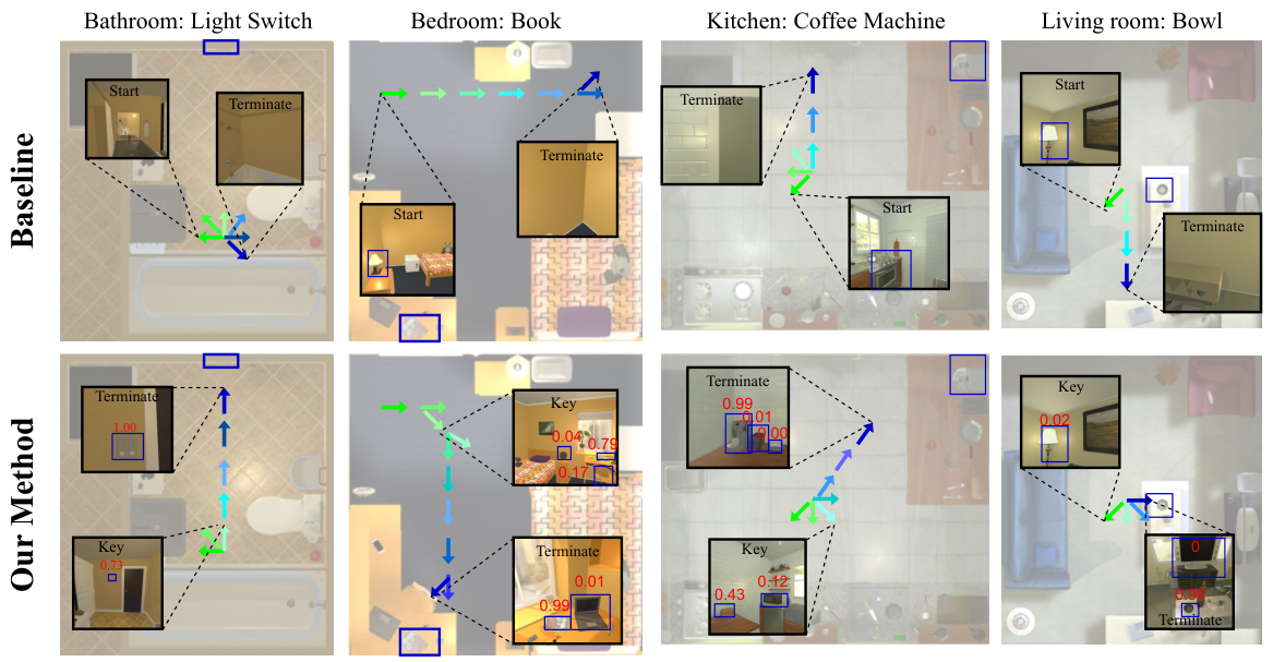
We visualize the navigation effect of the agent in Figure 5. The direction and stop timing of the rotation are critical, as seen in the trajectories of the success and failure cases. These two decisions are mainly determined by the agent’s interpretation of the scene at keyframes when multiple objects can provide rich information. Our DOA graph-based method provides the agent with a more reasonable and unbiased attention allocation at these keyframes, allowing the algorithm to choose the correct rotation direction and stop timing.

6. Conclusion

Based on the analysis of the network structure and the failed navigation of previous methods, we identify the agent’s object attention bias problem in navigation tasks. To address this problem, we use a directed object attention (DOA) graph, which allows the agent to unbiasedly redistribute object attention. Cross-attention modules (UAIA and UAOA) between the object branch and image branch are designed according to the DOA graph. Our experimental results show that our approach can effectively address the object attention bias problem, greatly improving the agent’s navigation ability. Furthermore, we propose an adaptive branch energy distribution (ABED) method for optimizing the aggregation of branch features that performs well in complex models. It is worth noting that we prioritize simplicity in our approach. In future work, we will attempt to determine more concrete relationships between objects so that the agent’s navigation can be more clearly interpreted.

Acknowledgements.

This paper is supported by the National Natural Science Foundation of China under Grants 61733013, 62173248, 62073245. Suzhou Key Industry Technological Innovation-Core Technology R&D Program, No. SGC2021035.

References

(1)
Anderson et al. (2018) Peter Anderson, Angel Chang, Devendra Singh Chaplot, Alexey Dosovitskiy, Saurabh Gupta, Vladlen Koltun, Jana Kosecka, Jitendra Malik, Roozbeh Mottaghi, Manolis Savva, et al. 2018. On evaluation of embodied navigation agents. arXiv preprint arXiv:1807.06757 (2018).
Cadene et al. (2019) Remi Cadene, Corentin Dancette, Matthieu Cord, Devi Parikh, et al. 2019. Rubi: Reducing unimodal biases for visual question answering. Advances in neural information processing systems 32 (2019).
Chaplot et al. (2020) Devendra Singh Chaplot, Dhiraj Prakashchand Gandhi, Abhinav Gupta, and Russ R Salakhutdinov. 2020. Object goal navigation using goal-oriented semantic exploration. Advances in Neural Information Processing Systems 33 (2020), 4247–4258.
Deitke et al. (2020) Matt Deitke, Winson Han, Alvaro Herrasti, Aniruddha Kembhavi, Eric Kolve, Roozbeh Mottaghi, Jordi Salvador, Dustin Schwenk, Eli VanderBilt, Matthew Wallingford, et al. 2020. Robothor: An open simulation-to-real embodied ai platform. In Proceedings of the IEEE/CVF Conference on Computer Vision and Pattern Recognition. 3164–3174.
Dosovitskiy et al. (2021) Alexey Dosovitskiy, Lucas Beyer, Alexander Kolesnikov, Dirk Weissenborn, Xiaohua Zhai, Thomas Unterthiner, Mostafa Dehghani, Matthias Minderer, Georg Heigold, Sylvain Gelly, Jakob Uszkoreit, and Neil Houlsby. 2021. An Image is Worth 16x16 Words: Transformers for Image Recognition at Scale. In 9th International Conference on Learning Representations, ICLR 2021, Virtual Event, Austria, May 3-7, 2021.
Du et al. (2020) Heming Du, Xin Yu, and Liang Zheng. 2020. Learning Object Relation Graph and Tentative Policy for Visual Navigation. In Computer Vision – ECCV 2020: 16th European Conference, Glasgow, UK, August 23–28, 2020, Proceedings, Part VII (Glasgow, United Kingdom). 19–34.
Fang et al. (2021) Qiang Fang, Xin Xu, Xitong Wang, and Yujun Zeng. 2021. Target-driven visual navigation in indoor scenes using reinforcement learning and imitation learning. CAAI Transactions on Intelligence Technology (2021).
Gao et al. (2021) Chen Gao, Jinyu Chen, Si Liu, Luting Wang, Qiong Zhang, and Qi Wu. 2021. Room-and-object aware knowledge reasoning for remote embodied referring expression. In Proceedings of the IEEE/CVF Conference on Computer Vision and Pattern Recognition. 3064–3073.
Geirhos et al. (2019) Robert Geirhos, Patricia Rubisch, Claudio Michaelis, Matthias Bethge, Felix A Wichmann, and Wieland Brendel. 2019. ImageNet-trained CNNs are biased towards texture; increasing shape bias improves accuracy and robustness. In International Conference on Learning Representations.
He et al. (2016) Kaiming He, Xiangyu Zhang, Shaoqing Ren, and Jian Sun. 2016. Deep residual learning for image recognition. In Proceedings of the IEEE conference on computer vision and pattern recognition. 770–778.
Khosla et al. (2012) Aditya Khosla, Tinghui Zhou, Tomasz Malisiewicz, Alexei A. Efros, and Antonio Torralba. 2012. Undoing the Damage of Dataset Bias. In Computer Vision – ECCV 2012. Springer Berlin Heidelberg, Berlin, Heidelberg, 158–171.
Kingma and Ba (2015) Diederik P. Kingma and Jimmy Ba. 2015. Adam: A Method for Stochastic Optimization. In 3rd International Conference on Learning Representations, ICLR 2015, San Diego, CA, USA, May 7-9, 2015, Conference Track Proceedings, Yoshua Bengio and Yann LeCun (Eds.).
Kolve et al. (2017) Eric Kolve, Roozbeh Mottaghi, Winson Han, Eli VanderBilt, Luca Weihs, Alvaro Herrasti, Daniel Gordon, Yuke Zhu, Abhinav Gupta, and Ali Farhadi. 2017. AI2-THOR: An Interactive 3D Environment for Visual AI. arXiv (2017).
Kozachenko and Leonenko (1987) Lyudmyla F Kozachenko and Nikolai N Leonenko. 1987. Sample estimate of the entropy of a random vector. Problemy Peredachi Informatsii 23, 2 (1987), 9–16.
Li et al. (2021b) Rongjie Li, Songyang Zhang, Bo Wan, and Xuming He. 2021b. Bipartite graph network with adaptive message passing for unbiased scene graph generation. In Proceedings of the IEEE/CVF Conference on Computer Vision and Pattern Recognition. 11109–11119.
Li et al. (2021a) Weijie Li, Xinhang Song, Yubing Bai, Sixian Zhang, and Shuqiang Jiang. 2021a. ION: Instance-level Object Navigation. In Proceedings of the 29th ACM International Conference on Multimedia. 4343–4352.
Li et al. (2018) Yingwei Li, Yi Li, and Nuno Vasconcelos. 2018. Resound: Towards action recognition without representation bias. In Proceedings of the European Conference on Computer Vision (ECCV). 513–528.
Li and Vasconcelos (2019) Yi Li and Nuno Vasconcelos. 2019. Repair: Removing representation bias by dataset resampling. In Proceedings of the IEEE/CVF Conference on Computer Vision and Pattern Recognition. 9572–9581.
Lin et al. (2017) Tsung-Yi Lin, Priya Goyal, Ross Girshick, Kaiming He, and Piotr Dollár. 2017. Focal loss for dense object detection. In Proceedings of the IEEE international conference on computer vision. 2980–2988.
Mirowski et al. (2017) Piotr Mirowski, Razvan Pascanu, Fabio Viola, Hubert Soyer, Andrew J Ballard, Andrea Banino, Misha Denil, Ross Goroshin, Laurent Sifre, Koray Kavukcuoglu, et al. 2017. Learning to navigate in complex environments. In 5th International Conference on Learning Representations.
Misra et al. (2016) Ishan Misra, C Lawrence Zitnick, Margaret Mitchell, and Ross Girshick. 2016. Seeing through the human reporting bias: Visual classifiers from noisy human-centric labels. In Proceedings of the IEEE Conference on Computer Vision and Pattern Recognition. 2930–2939.
Mnih et al. (2016) Volodymyr Mnih, Adria Puigdomenech Badia, Mehdi Mirza, Alex Graves, Timothy Lillicrap, Tim Harley, David Silver, and Koray Kavukcuoglu. 2016. Asynchronous methods for deep reinforcement learning. In International conference on machine learning. PMLR, 1928–1937.
Mnih et al. (2015) Volodymyr Mnih, Koray Kavukcuoglu, David Silver, Andrei A Rusu, Joel Veness, Marc G Bellemare, Alex Graves, Martin Riedmiller, Andreas K Fidjeland, Georg Ostrovski, et al. 2015. Human-level control through deep reinforcement learning. nature 518, 7540 (2015), 529–533.
Moghaddam et al. (2022) Mahdi Kazemi Moghaddam, Ehsan Abbasnejad, Qi Wu, Javen Qinfeng Shi, and Anton Van Den Hengel. 2022. ForeSI: Success-Aware Visual Navigation Agent. In Proceedings of the IEEE/CVF Winter Conference on Applications of Computer Vision. 691–700.
Moudgil et al. (2021) Abhinav Moudgil, Arjun Majumdar, Harsh Agrawal, Stefan Lee, and Dhruv Batra. 2021. SOAT: A Scene-and Object-Aware Transformer for Vision-and-Language Navigation. Advances in Neural Information Processing Systems 34 (2021).
Nair and Hinton (2010) Vinod Nair and Geoffrey E Hinton. 2010. Rectified linear units improve restricted boltzmann machines. In Icml.
Qi et al. (2020) Yuankai Qi, Qi Wu, Peter Anderson, Xin Wang, William Yang Wang, Chunhua Shen, and Anton van den Hengel. 2020. Reverie: Remote embodied visual referring expression in real indoor environments. In Proceedings of the IEEE/CVF Conference on Computer Vision and Pattern Recognition. 9982–9991.
Qiu et al. (2020) Yiding Qiu, Anwesan Pal, and Henrik I Christensen. 2020. Target driven visual navigation exploiting object relationships. arXiv preprint arXiv:2003.06749 2 (2020), 7.
Ren et al. (2015) Shaoqing Ren, Kaiming He, Ross Girshick, and Jian Sun. 2015. Faster r-cnn: Towards real-time object detection with region proposal networks. Advances in neural information processing systems 28 (2015).
Savva et al. (2019) Manolis Savva, Abhishek Kadian, Oleksandr Maksymets, Yili Zhao, Erik Wijmans, Bhavana Jain, Julian Straub, Jia Liu, Vladlen Koltun, Jitendra Malik, et al. 2019. Habitat: A platform for embodied ai research. In Proceedings of the IEEE/CVF International Conference on Computer Vision. 9339–9347.
Su et al. (2021) Jianlin Su, Yu Lu, Shengfeng Pan, Bo Wen, and Yunfeng Liu. 2021. Roformer: Enhanced transformer with rotary position embedding. arXiv preprint arXiv:2104.09864 (2021).
Tang et al. (2020) Kaihua Tang, Yulei Niu, Jianqiang Huang, Jiaxin Shi, and Hanwang Zhang. 2020. Unbiased scene graph generation from biased training. In Proceedings of the IEEE/CVF conference on computer vision and pattern recognition. 3716–3725.
Torralba and Efros (2011) Antonio Torralba and Alexei A Efros. 2011. Unbiased look at dataset bias. In CVPR 2011. IEEE, 1521–1528.
Vaswani et al. (2017) Ashish Vaswani, Noam Shazeer, Niki Parmar, Jakob Uszkoreit, Llion Jones, Aidan N Gomez, Łukasz Kaiser, and Illia Polosukhin. 2017. Attention is all you need. Advances in neural information processing systems 30 (2017).
Wortsman et al. (2019) Mitchell Wortsman, Kiana Ehsani, Mohammad Rastegari, Ali Farhadi, and Roozbeh Mottaghi. 2019. Learning to learn how to learn: Self-adaptive visual navigation using meta-learning. In Proceedings of the IEEE/CVF Conference on Computer Vision and Pattern Recognition. 6750–6759.
Wu et al. (2018) Yi Wu, Yuxin Wu, Georgia Gkioxari, and Yuandong Tian. 2018. Building generalizable agents with a realistic and rich 3d environment. arXiv preprint arXiv:1801.02209 (2018).
Yang et al. (2019) Wei Yang, Xiaolong Wang, Ali Farhadi, Abhinav Gupta, and Roozbeh Mottaghi. 2019. Visual Semantic Navigation using Scene Priors. In 7th International Conference on Learning Representations, ICLR 2019, New Orleans, LA, USA, May 6-9, 2019.
Ye et al. (2021) Joel Ye, Dhruv Batra, Abhishek Das, and Erik Wijmans. 2021. Auxiliary tasks and exploration enable objectgoal navigation. In Proceedings of the IEEE/CVF International Conference on Computer Vision. 16117–16126.
Zemel et al. (2013) Rich Zemel, Yu Wu, Kevin Swersky, Toni Pitassi, and Cynthia Dwork. 2013. Learning fair representations. In International conference on machine learning. PMLR, 325–333.
Zhang et al. (2021) Sixian Zhang, Xinhang Song, Yubing Bai, Weijie Li, Yakui Chu, and Shuqiang Jiang. 2021. Hierarchical Object-to-Zone Graph for Object Navigation. In Proceedings of the IEEE/CVF International Conference on Computer Vision. 15130–15140.
Zhou et al. (2021) Haoyi Zhou, Shanghang Zhang, Jieqi Peng, Shuai Zhang, Jianxin Li, Hui Xiong, and Wancai Zhang. 2021. Informer: Beyond efficient transformer for long sequence time-series forecasting. In Proceedings of AAAI.
Zhou et al. (2020) Li Zhou, Tingyu Wang, Hong Qu, Li Huang, and Yuguo Liu. 2020. A weighted GCN with logical adjacency matrix for relation extraction. In ECAI 2020. IOS Press, 2314–2321.
Zhu et al. (2021) Fengda Zhu, Xiwen Liang, Yi Zhu, Qizhi Yu, Xiaojun Chang, and Xiaodan Liang. 2021. SOON: scenario oriented object navigation with graph-based exploration. In Proceedings of the IEEE/CVF Conference on Computer Vision and Pattern Recognition. 12689–12699.

Table 7. Goal-driven navigation datasets. The attributes include: Instruction: type of instruction; Observation: views that the agent can use; Scenes: number of different scenes in the simulation; Real-Picture: pictures taken in real environments; Interaction: whether the agent moves or changes the object state; Navigation Graph: the presumptions of the known environmental topologies; and Realistic: resemblance to real-world environments.

Dataset	Instruction	Observation	Scenes	Real-Picture	Interaction	Navigation Graph	Realistic
House3D (2018) (Wu et al. 2018)	room name	single view	45622				weak
Habitat (2019) (Savva et al. 2019)	object name	single view	90	✓			moderate
AI2-Thor (2019) (Kolve et al. 2017)	object name	single view	120		✓		moderate
RoboTHOR (2020) (Deitke et al. 2020)	object name	single view	89				strong
REVERIE (2020) (Qi et al. 2020)	task language	panoramas	90	✓		✓	weak
FAO (2021) (Zhu et al. 2021)	locate language	panoramas	90	✓		✓	weak

Appendix A More Analyses on Datasets

Table 7 summarizes the most commonly used datasets for object navigation tasks. We compare these datasets in terms of the instructions given, the views used, the variety and realism of the scenes, the ability of the agent to interact, the presence or absence of a predefined navigation map, and the ability to map the environment to reality. Since our method is based on the input of object names and single views, in addition to using the AI2-Thor dataset discussed in the main text, we also conduct experiments on the RoboTHOR dataset.

Appendix B Object Attention Bias

Table 8. Comparison of introducing object semantics and position into the GCN node features (%).

GCN	Semantics	Position	ALL			L>=5			Episode Length
GCN	Semantics	Position	SR	SPL	SAE	SR	SPL	SAE	Episode Length
✓			$68.53_{\pm 1.32}$	$37.50_{\pm 1.01}$	$25.98_{\pm 0.96}$	$60.27_{\pm 1.67}$	$36.61_{\pm 1.12}$	$27.68_{\pm 1.31}$	$27.25_{\pm 0.87}$
✓	✓		$69.45_{\pm 0.76}$	$37.36_{\pm 0.99}$	$27.65_{\pm 1.31}$	$61.02_{\pm 1.09}$	$37.15_{\pm 0.32}$	$29.30_{\pm 1.78}$	$26.02_{\pm 0.86}$
✓		✓	$69.12_{\pm 0.90}$	$38.19_{\pm 0.56}$	$27.23_{\pm 0.88}$	$60.76_{\pm 1.78}$	$37.94_{\pm 1.12}$	$29.01_{\pm 1.34}$	$25.33_{\pm 1.24}$

We discover the object attention bias problem during our research on object features GCN, as discussed in (Du et al. 2020; Zhang et al. 2021). In the main text, we briefly analyzed this problem. Here, we elaborate on why GCNs have issues with object attention bias. As shown in Figure 6, the object GCN is divided into two stages: (i) Generating the adjacency matrix, and (ii) Transferring information between objects using the adjacency matrix. The object attention bias problem arises in both stages.

B.1. Bias in Generating the Adjacency Matrix

The adjacency matrix is generated based on the relationships between the bounding boxes of objects, which defines the correlation between objects. However, after training, the network determines the importance of an object based on the size of its bounding box and its confidence score, thereby ignoring the category and position of the object, which are both more important features. In Table 8, we explicitly add the object semantics and position to the GCN node features of the HOZ (Zhang et al. 2021) method and find that the agent’s navigation performance improves slightly. The results show that it is important for the agent to pay more attention to what the object is and where the objects are; however, this feature introduction cannot effectively resolve the object attention bias generated during training the GCN. Furthermore, since the agent usually can view only a few objects at a time, the object features graph is sparse and thus more susceptible to bias. Figure 7 shows the weights on the edge connecting some specified objects and other objects in the adjacency matrix when searching for different targets in the same bedroom scene. Due to the sparsity of the objects, most edge weights are 0. It is worth noting that regardless of what object is being searched for, the floor lamp has a high connection weight with the other objects. This illustrates that the volume and clarity of the floor lamp cause the agent to overestimate its importance in the bedroom scene.

B.2. Bias in Convolutional Object Visual Features

The convolution of object visual features with a biased adjacency matrix clearly leads to biased results. However, in this section, we discuss that even if the object bias in the adjacency matrix is not considered, the convolution of the object visual features can also generate this bias. Figure 8 shows the original images of the objects and their information entropy calculated by the k-nearest neighbor (KNN) method (Kozachenko and Leonenko 1987). As a result, even if an object is recognized, it is likely to be ignored due to the disadvantage of its feature information richness.

Appendix C More Ablation Experiments

Table 9. Navigation performance after replacing some modules in the model (%). Our Best Model represents the model used in our main text.

Module Replacement		ALL			L>=5			Episode Length
Module Replacement		SR	SPL	SAE	SR	SPL	SAE	Episode Length
Our Best Model		$74.32_{\pm 0.89}$	$40.27_{\pm 1.01}$	$29.79_{\pm 0.80}$	$67.88_{\pm 1.05}$	$40.36_{\pm 1.23}$	$32.56_{\pm 1.76}$	$22.86_{\pm 1.32}$
Backbone	ResNet50	$74.12_{\pm 1.23}$	$35.98_{\pm 1.56}$	$28.76_{\pm 0.90}$	$66.77_{\pm 1.12}$	$33.50_{\pm 1.27}$	$32.34_{\pm 1.52}$	$27.96_{\pm 0.88}$
Backbone	ResNet101	$70.21_{\pm 1.45}$	$35.56_{\pm 1.07}$	$26.77_{\pm 1.34}$	$65.43_{\pm 0.81}$	$31.45_{\pm 1.23}$	$29.70_{\pm 0.99}$	$28.21_{\pm 1.29}$
Object Detector	Ground Truth	$76.12_{\pm 1.48}$	$59.12_{\pm 1.10}$	$30.98_{\pm 1.27}$	$69.07_{\pm 0.65}$	$54.93_{\pm 1.35}$	$35.15_{\pm 0.93}$	$17.45_{\pm 1.05}$
Pixel Index Emb.	No	$74.54_{\pm 1.20}$	$38.14_{\pm 0.82}$	$29.13_{\pm 1.03}$	$67.76_{\pm 1.38}$	$38.55_{\pm 1.07}$	$32.67_{\pm 1.21}$	$24.21_{\pm 0.94}$
	2-D	$74.29_{\pm 1.22}$	$40.54_{\pm 0.79}$	$29.38_{\pm 1.62}$	$67.81_{\pm 1.09}$	$40.35_{\pm 1.67}$	$32.29_{\pm 1.24}$	$22.59_{\pm 0.93}$
	Relative	$74.10_{\pm 0.85}$	$40.34_{\pm 1.07}$	$29.33_{\pm 1.55}$	$67.45_{\pm 1.38}$	$40.19_{\pm 1.43}$	$31.98_{\pm 1.33}$	$23.45_{\pm 0.74}$
DOA Graph	Undirected	$73.15_{\pm 1.17}$	$38.44_{\pm 1.26}$	$27.43_{\pm 1.63}$	$66.33_{\pm 1.44}$	$37.60_{\pm 1.10}$	$30.95_{\pm 1.28}$	$26.84_{\pm 1.36}$

C.1. Choice of Backbone

In the main text, we use ResNet18 as the backbone network for extracting the global image features. Additionally, we also experiment with backbones of different depths. Table 9 shows the results after we replace the backbone with ResNet50 and ResNet101. Compared to ResNet18, the use ResNet50 decreases the SR, SPL and SAE by 0.20/1.11, 4.29/6.86 and 1.03/0.22 (ALL/L>=5,%). The losses in the SR, SPL and SAE when using ResNet101 as the backbone network are even greater. It is clear that the SPL and the episode length are most severely affected. The explanation may be that excessive high-level global image information degrades local information, thereby weakening the effect of cross-attention with the object branch and impairing the action selection at each step in the overall path. As a result, the navigation distance is greatly increased, which affects the SPL.

C.2. Importance of Accurate Object Information

In our model, we apply Faster-RCNN (Ren et al. 2015), which was trained on 50% (Zhang et al. 2021) of the training data from the AI2-Thor dataset, to extract the object information. Table 9 shows the results when the ground truth object information is used as the input of the object branch, improving the SR, SPL and SAE by 1.80/1.19, 18.85/14.57 and 1.19/2.59 (ALL/L >=5, %). Similar to the conclusion presented in (Zhang et al. 2021), the ground truth object information has a strong effect on the optimization of navigation path. Notably, our DOA graph method significantly increases the upper bound of the model, and when more accurate and efficient features are used, our model performs better.

Table 10. Comparision with SOTA methods in RoboTHOR (Deitke et al. 2020) (%)

Method	ALL			L>=5			Episode Length
Method	SR	SPL	SAE	SR	SPL	SAE	Episode Length
Random	$0.00_{\pm 0.00}$	$0.00_{\pm 0.00}$	$0.00_{\pm 0.00}$	$0.00_{\pm 0.00}$	$0.00_{\pm 0.00}$	$0.00_{\pm 0.00}$	$3.01_{\pm 0.32}$
LSTM+A3C	$21.35_{\pm 0.23}$	$9.28_{\pm 0.54}$	$7.03_{\pm 0.34}$	$11.21_{\pm 0.41}$	$7.65_{\pm 0.26}$	$6.33_{\pm 0.86}$	$87.29_{\pm 1.95}$
SP (Yang et al. 2019)	$27.43_{\pm 0.60}$	$17.49_{\pm 0.36}$	$15.21_{\pm 0.33}$	$20.98_{\pm 0.97}$	$16.03_{\pm 0.48}$	$13.99_{\pm 0.44}$	$68.18_{\pm 1.27}$
SAVN (Wortsman et al. 2019)	$28.97_{\pm 0.84}$	$16.59_{\pm 0.65}$	$13.21_{\pm 0.37}$	$22.89_{\pm 0.98}$	$15.21_{\pm 0.41}$	$13.77_{\pm 0.30}$	$67.22_{\pm 0.93}$
ORG (Du et al. 2020)	$30.51_{\pm 0.21}$	$18.62_{\pm 0.19}$	$14.71_{\pm 0.47}$	$23.89_{\pm 0.55}$	$14.91_{\pm 0.38}$	$13.73_{\pm 0.50}$	$69.17_{\pm 2.13}$
HOZ (Zhang et al. 2021)	$31.67_{\pm 0.87}$	$19.02_{\pm 0.49}$	$15.44_{\pm 0.63}$	$24.32_{\pm 0.48}$	$14.81_{\pm 0.23}$	$14.22_{\pm 0.88}$	$66.26_{\pm 1.88}$
Ours (Baseline)	$31.92_{\pm 0.37}$	$18.88_{\pm 0.18}$	$16.37_{\pm 0.33}$	$24.72_{\pm 0.26}$	$15.56_{\pm 0.35}$	$15.18_{\pm 0.61}$	$65.31_{\pm 1.69}$
Ours (DOA+ABED)	$\textbf{36.22}_{\pm 0.36}$	$\textbf{22.12}_{\pm 0.42}$	$\textbf{18.70}_{\pm 0.59}$	$\textbf{30.16}_{\pm 0.28}$	$\textbf{18.32}_{\pm 0.34}$	$\textbf{19.21}_{\pm 0.52}$	$\textbf{61.24}_{\pm 1.23}$

Figure 12. The performance of the agent on the training and validation datasets during training. The agent is tested on the validation dataset every

10^{5}

navigation episodes.

C.3. Pixel Index Embedding

In the UAIA module, the pixel index embeddings provide each pixel’s position token, which is important in the muti-head attention mechanism. In Table 9, we compare the results of the following encodings:

1)

Providing no positional information (No): Considering the image feature maps as a bag of pixel vectors.
2)

1-dimensional pixel index embedding (Our Best Model): Considering the image feature maps as a sequence of pixel vectors in order.
3)

2-dimensional pixel index embedding (2-D): Considering the image feature maps as a grid of pixel vectors in two dimensions.
4)

Relative pixel index embedding (Relative): Considering the relative distance between pixels rather than their absolute position to encode the spatial information.

The results show that without pixel index embeddings, the SPL is reduced by approximately 2%. However, when using 1-D, 2-D or relative pixel index embeddings, the effect is essentially the same. We speculate that this occurs because we perform position embeddings on feature maps with smaller spatial dimensions instead of on the original image, which has larger spatial dimensions. Hence, the process of learning the spatial relations at this resolution is equally easy for the different positional encoding strategies.

C.4. Directivity in DOA Graph

In the main text, we repeatedly emphasize that our proposed DOA graph is a directed graph; thus, the correlation between object B and object A when searching for object A is different from the correlation between object A and object B when searching for object B. Table 9 illustrates that the navigation improvement decreases significantly when the DOA graph is an undirected graph. Fundamentally, the directed object graph follows the relative relationships between objects, while the undirected object graph follows the absolute relationships between objects. The absolute object relationships reduce the adaptability of the agent in modeling object relationships in different scenes, thus reducing its performance in unseen environments.

C.5. Hyperparameters

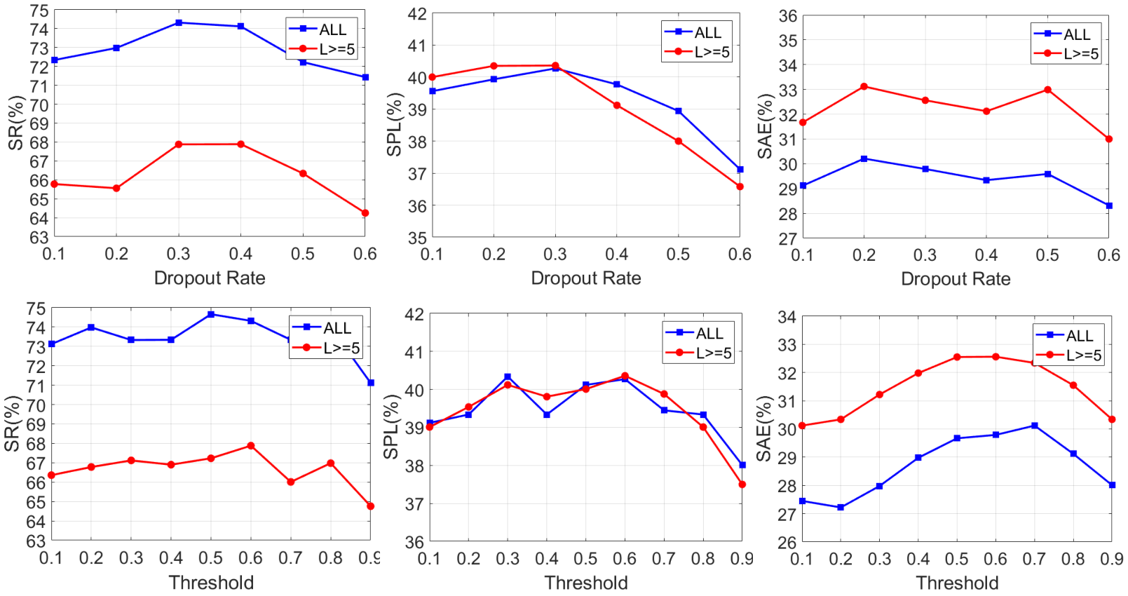
The hyperparameters are also an important factor in determining the final navigation performance of the agent. However, due to the complexity of the object navigation task, small changes in the network structure have a considerable impact on the selection of the hyperparameters. Therefore, as shown in Figure 9, we conduct extensive experiments on the final model with different dropout rates and confidence filter thresholds. The experimental results show that when a hyperparameter changes, the change rules of the three metrics (the SR, SPL and SAE) differ. Thus, we consider all three metrics when choosing the most appropriate hyperparameters for our model.

Appendix D More comparisons with the related works

D.1. Comparisons in RoboTHOR Dataset

We compare our method with the other related works on the AI2-Thor dataset in the main text. We consider that the scenes in AI2-Thor are relatively simple, so the RoboTHOR (Deitke et al. 2020) dataset is used to verify the effectiveness of our method in complex environment. RoboTHOR has public 75 apartments, we choose 60 for training, 5 for validation and 10 for testing.

Table 10 illustrates the performance of our method and other related methods on the RoboTHOR. Obviously, the various metrics on the RoboTHOR are generally low, which indicates that object navigation on RoboTHOR is much more difficult than AI2-Thor. Moreover, The episode length of navigation on RoboTHOR is 3 times that of AI2-Thor, which indicates that each navigation scene in RoboTHOR is much more complicated. Nevertheless, out method still outperforms the proposed baseline with an obvious margin by 4.3/5.44, 3.24/2.76 and 2.33/4,03 in SR, SPL and SAE (ALL/L>=5, %).

Appendix E Qualitative Results

E.1. The DOA Graph Visualization

Our proposed DOA graph has two parts: the intrinsic object graph, which represents the ubiquitous inherent relationship between the objects, and the view adaptive graph, which changes adaptively according to the input at each timestep. A weighted sum of the two graphs gives the attention score assigned to each object at this timestep. Figure 10 shows the adjacency matrix of the two graphs. For the adjacency matrix of the intrinsic object graph, the largest value is on the diagonal, indicating that the self-connecting edge has the largest weight. This result is consistent with our assumption that when the target object is identified, most of the attention is focused on the target object. For the adjacency matrix of the view adaptive graph, we randomly select the view adaptive attention when looking for different targets as a column. Interestingly, at each timestamp in the view adaptive graph, only one object’s attention weight is close to 1, while the other object’s attention weight is close to 0. We speculate that because there are often very few objects observed at each timestamp and most of these objects are essentially irrelevant to the target object, the view adaptive graph directs all attention to the most important object. In the weighted sum of the two graphs, the weight of the intrinsic object graph is 0.95, while the weight of the view adaptive graph is only 0.05. Therefore, although the attention distribution of the view adaptive graph is extreme, it does not affect the robustness of the overall attention distribution. In contrast, the attention concentration in the view adaptive graph reasonably increases the weight of important objects in view.

E.2. Training Process

Figure 12 shows the agent’s navigation success rate (SR) on the training and validation datasets during reinforcement learning. We observe that after the agent has learned 0.5 M episodes, the navigation success rate greatly improved, and the SR curve converged after 2.5 M episodes. Due to computational resource constraints, we train our models on 3 M navigation episodes in our usual experiments. To obtain the best model of the current network structure, we can increase the number of training episodes to 6 M.

E.3. Navigation Trajectory in RoboTHOR

Since the AI2-Thor dataset only includes simple room constructions, we also use the RoboTHOR dataset, which includes more complex indoor environments, to verify the effectiveness of our model. As shown in Figure 11, in the RoboTHOR environment, the agent spends more time searching for the target object. Compared with the baseline, the agent can approach the target step-by-step in a continuous exploration with our proposed DOA graph.