Optimal Lane-Free Crossing of CAVs through IntersectionsManuscript received , 2021; revised . Corresponding author: Mahdi Amouzadi (email: m.amouzadi@sussex.ac.uk).

Fig. 1 illustrates an example layout of a lane-free and signal-free intersection. The figure includes three CAVs which are moving from their initial points, depicted with the most solid colour, towards their intended destinations which are with the most transparent colour. The intersection comprises of four approaches, each of them has a separate incoming and outgoing lane. In a lane-free intersection, vehicles can freely change their lanes in favour of faster crossing through the intersection. For instance, Fig. 1 shows the green CAV overtakes the black CAV by using the opposite lane. It is worth noting that the intersection does not have traffic lights because the CAVs can directly communicate their states and intentions. In addition, all vehicles are of CAV type and no human-driven vehicle nor pedestrian are considered. In this study, there is a coordinator that receives all the information from the CAVs and centrally control them to efficiently and safely cross the intersection. This fully-connected and centralised topology provides the optimal solution as the benchmark for testing any decentralised strategies.

The black and green CAVs also show the collision avoidance. In this regard, the expression $-b_{i}^{\top}\lambda_{ij}-b_{j}^{\top}\lambda_{ji}$ is the dual representation of the distance between a pair of CAVs and $S_{ij}$ is the separating hyperplane placed between them. Similarly, the red CAV and the highlighted road boundary show the road boundary avoidance. $-b_{i}^{\top}\lambda_{ir}-b_{r}^{\top}\lambda_{ri}$ is the dual representation of distance between a CAV and a road boundary and $S_{ir}$ is the separating hyperplane between them. These equations are further explained in section III.

This study represents the lateral behaviour of CAVs with the bicycle model [24]. The bicycle model consists of two degree-of-freedom (DoF) which are sideslip angle $\beta_{i}$ and yaw rate $r_{i}$, as in Fig. 2(a). The model also includes an additional DoF for the longitudinal velocity $V_{i}$. The equations of these DoFs along with other three to model the ground-fixed location, construct a set of differential equations to represent $\text{CAV}_{i}$ as follows:

where $\textbf{x}=[r_{i},\beta_{i},V_{i},x_{i},y_{i},\theta_{i}]^{T}$ and $\textbf{u}=[a_{i},\delta_{i}]^{T}$ are, respectively, the system states and control inputs of $\text{CAV}_{i}$. $\textbf{z}_{i}=[x_{i},y_{i},\theta_{i}]^{T}$ refers to the pose of $\text{CAV}_{i}$ in non-inertial reference system. $a_{i}(t)$ and $\delta_{i}(t)$ are, respectively, the acceleration ($m^{2}$) and steering angle ($rad$) of the vehicle. The constants $m$ and $I_{z}$ denote mass ($kg$) and moment of inertia ($kg.m^{2}$) of the vehicle. $t_{0}$ and $t_{f}$ represent the starting and final time ($s$) of crossing the intersection. The vehicle parameters $\tilde{N_{r}}$, $N_{\beta}$, $N_{\delta}$, $\tilde{Y_{r}}$, $Y_{\beta}$ and $Y_{\delta}$ are calculated as follows [24]:

where $C_{F}$ and $C_{R}$ are, respectively, the cornering stiffness of the front and rear tyres. $l_{f}$ and $l_{r}$ are distance of the front and rear axis from center of gravity of the vehicle.

To ensure CAVs drive within their dynamic limitations, the following constraints are enforced for each $\text{CAV}_{i}$:

where $\overline{.}$ and $\underline{.}$ are, respectively, the upper and lower boundaries.

This study represents each $\text{CAV}_{i}$, when $i\in\{1..N\}$ and $N$ is the total number of CAVs, as a rectangular polytope $\tilde{\beta}_{i}$ (i.e., a convex set) that is the intersection area of half-space linear inequalities $\tilde{A}_{i}X\leq\tilde{b}_{i}$ at the origin, where $X=[x,y]^{T}$ is a Cartesian point. In this paper, all CAVs have the same size which are defined with:

where $l$ and $d$ denote, respectively, the wheelbase and track of CAVs.

As $\text{CAV}_{i}$ moves to a new pose $\textbf{z}_{i}(t)=[x_{i}(t),y_{i}(t),\theta_{i}(t)]^{T}$, the original polytope $\tilde{\beta}_{i}$ of the CAV is transformed to $\beta_{i}$ as follows:

where:

Fig. 2(b) provides a graphical representation of (4).

Road boundaries are also modelled as convex polytopic sets $O_{r}$, when $r\in\{1..N_{r}\}$ and $N_{r}$ is the total number of road boundaries which is 4 for four-legged intersections.

Based on these representations, there is no collision between $\text{CAV}_{i}$ and $\text{CAV}_{j}$ iff $\beta_{i}(\textbf{z}_{i};t)\cap\beta_{j}(\textbf{z}_{j};t)=\emptyset,\forall t\in[t_{0},t_{f}]$. Similarly, CAVs do not collide with road boundaries when the intersection of their sets is always empty, i.e. $\beta_{i}(\textbf{z}_{i};t)\cap O_{r}=\emptyset,\forall t\in[t_{0},t_{f}]$.

To avoid collisions between any $\text{CAV}_{i}$ and $\text{CAV}_{j}$ $\forall i\neq j\in\{1..N\}$, their polytopic sets should not intersect, i.e. $\beta_{i}\cap\beta_{j}=\emptyset$ where $\beta_{i}=\{\text{X}\in\mathbb{R}^{2}|A_{i}\text{X}\leq b_{i}\}$ and $\beta_{j}=\{\text{Y}\in\mathbb{R}^{2}|A_{j}\text{Y}\leq b_{j}\}$. However, these are non-convex and non-differentiable conditions and enforcing them as constraints in an OCP will make the problem non-convex and difficult solve. To preserve differentiability and continuity, $\beta_{i}\cap\beta_{j}=\emptyset$ is replaced by the following sufficient condition which has negligible effect on the optimality of the solution for small values of $d_{min}$ [25]:

where $d_{min}$ is the minimum safe distance between CAVs.

It is known that the problem of finding the minimum distance between a polytope $\beta_{i}$ and another given polytope $\beta_{j}$ is convex [26]. Therefore the substituted sufficient condition, $dist(\beta_{i},\beta_{j})\geq d_{min}$, is convex and since $\beta_{j}$ is not an empty set, the strong duality holds [25]. This means that the solution of the primal problem $dist(\beta_{i},\beta_{j})\geq d_{min}$ is the same as the one of its dual problem which is as follows:

where $\lambda_{ij}$, $\lambda_{ji}$, and $s_{ij}$ are the dual variables and $A_{i}$ and $b_{i}$ are as in (5) (the deviation of dual problem (7) from primal problem (III-A) is shown in [27]).

Combining (7) with (III-A), the objective function of (7) subject to its constraints must be greater than or equal to $d_{min}$ in order to avoid collisions. However, (7) can be substituted by $\{\exists\lambda_{ij}\geq 0,\lambda_{ji}\geq 0,s_{ij}:-b_{i}^{\top}\lambda_{ij}-b_{j}^{\top}\lambda_{ji}\geq d_{cmin},A_{i}^{\top}\lambda_{ij}+s_{ij}=0,A_{j}^{\top}\lambda_{ji}-s_{ij}=0,\left\lVert s_{ij}\right\rVert_{2}\leq 1\}$ because the existence of a feasible solution $\lambda_{ij,feas}$, $\lambda_{ji,feas}$, and $s_{ij,feas}$ where $-b_{i}^{\top}\lambda_{ij,feas}-b_{j}^{\top}\lambda_{ji,feas}\geq d_{min}$ is a sufficient condition to ensure $dist(\beta_{i},\beta_{j})\geq d_{min}$, i.e. to avoid collisions [27]. As seen in Fig. 1, $S_{ij}$ is a separating hyperplane between $\text{CAV}_{i}$ and $\text{CAV}_{j}$ and $S_{ij}$ = $S_{ji}$.

Each $\text{CAV}_{i}$ must also avoid all the road boundaries, i.e. $\beta_{i}\cap O_{r}=\emptyset$ where $\beta_{i}=\{\text{X}\in\mathbb{R}^{2}|A_{i}\text{X}\leq b_{i}\}$ and $O_{r}=\{\text{Y}\in\mathbb{R}^{2}|A_{r}\text{Y}\leq b_{r}\}$. Similar to section III-A collision avoidance between CAVs, $\beta_{i}\cap O_{r}=\emptyset$ is replaced by the following sufficient condition:

where $d_{rmin}$ is the minimum safety distance between CAVs and road boundaries.

The dual problem of (III-B) is then substituted with the sufficient condition $\{\exists\lambda_{ir}\geq 0,\lambda_{ri}\geq 0,s_{ir}:-b_{i}^{\top}\lambda_{ir}-b_{r}^{\top}\lambda_{ri}\geq d_{rmin},A_{i}^{\top}\lambda_{ir}+s_{ir}=0,A_{j}^{\top}\lambda_{ri}-s_{ir}=0,\left\lVert s_{ir}\right\rVert_{2}\leq 1\}$ where $\lambda_{ir},\lambda_{ri}$, and $s_{ir}$ are the dual variables. $S_{ir}$ is the separating hyperplane between CAVs and road boundaries (see Fig. 1).

CAVs are expected to reach their terminal pose as fast as possible while consume energy as little as possible. Therefore, this paper proposes the objective function (9) that minimises the overall crossing time of all CAVs and the error between the current and final pose, as well as the energy consumption of each vehicle:

where $\alpha$, Q and $\gamma$ are the gain factors related to the crossing time, CAVs’ pose and energy consumption respectively. The gains are selected based on trail and error to best normalise the cost function. The expression $(t_{f}-t_{0})^{2}$ minimises the crossing time of all CAVs. The Lagrange term penalises the error between the current pose $\textbf{z}_{i}(t)$ and the final pose $\textbf{z}_{i}(t_{f})$ as well as the acceleration $a_{i}(t)^{2}$ of vehicles. The final pose of CAVs $\textbf{z}_{i}(t_{f})$ is directly imposed in the objective function and indicates the intended destination of each $\text{CAV}_{i}$.

Lane-free crossing of multiple CAVs through a signal-free intersection is formulated as the following optimal control problem:

where (10c) refers to the vehicle kinematics and (10d) and (10) denote, respectively, collision avoidance constraints of each CAV with others and with road boundaries.

As discussed in sections III-A and III-B, the non-differentiable and non-convex collision avoidance constraints (10d) and (10) are substituted by the dual problem of their sufficient conditions (III-A) and (III-B), and then (10) is reformulated as the following smooth and continuous problem, which is solvable by the state-of-the-art gradient-based algorithms:

where $A_{i}$ and $b_{i}$ are functions of each CAV’s pose $\textbf{z}_{i}(t)$, and present $\text{CAV}_{i}$ polytope at each time step $t$. Problem (11) is solved at time $t_{0}$ for $N$ CAVs until the terminal time $t_{f}$. The solution to this problem is optimal trajectories of the control signals $a_{i}(.)^{*}$ and $\delta_{i}(.)^{*}$ of each $\text{CAV}_{i}$ for each $t\in[t_{0},t_{f}]$, as well as a terminal time $t_{f}$. CAVs follow their calculated trajectories to arrive final destination at the terminal time $t_{f}$.

The initial pose $\textbf{z}_{i}$, i.e. initial position, heading angle and initial speed $V_{i}$ of all $\text{CAV}_{i}\>\forall i\in\{1..N\}$ within the control zone are known. The remaining of the states and the initial inputs to the CAVs are also assumed as zero. These initial conditions at $t=t_{0}$ are feasible solutions of the OCP.

This section compares the minimum crossing time of CAVs that can be achieved by the developed and benchmark algorithms. The acceleration gain $\gamma$ in (9) is set to zero to calculate the minimum-time travelling trajectories of CAVs. In other words, the energy consumption is not considered and CAVs only try to reach destinations as fast as possible, which makes the problem single objective.

Table III compares crossing time of CAVs when they are controlled by the developed and benchmark algorithms during test scenario one. The table also summarises energy consumption, the travelled distance and average and standard deviation of speed of CAVs. It is worth noting that the crossing time is measured as the time when all the CAVs are already arrived to their destinations. Also, the travelled distance and energy consumption are calculated for all the crossing CAVs.

As seen in Table III, crossing time of CAVs when they are controlled by the proposed algorithm is, respectively, up to $65\%$ (for 12 CAVs and in average $52\%$ for all number of crossing CAVs), and $54\%$ less than the case where CAVs are controlled by the reservation-based approach in [12] and the lane-free method in [14]. This is, of course, in cost of higher energy consumption, as the objective function of the proposed algorithm only considers minimisation of travelling time. The next subsection provides a detail analysis on energy consumption of different approaches, and shows that the proposed algorithm can still achieve significant improvement in crossing time while consuming the same amount of energy as the reservation-based method in [12].

It is also shown in Table III that, unlike the reservation-based strategy, the resulting crossing time of the proposed algorithm does not change regardless of number of crossing CAVs. There is a similar trend for the average and standard deviation of speed of CAVs when they are controlled by the developed strategy. Also, it is evident from Table III that the standard deviation of the speed of crossing CAVs when are controlled by the proposed algorithm is mostly less than the case when they are controlled by the reservation based strategy in [12]. Apparently, the smaller value of standard deviation of speed indicates a less diverge set of speeds (i.e., smoother travel) for the crossing CAVs.

Table IV shows crossing time, average and standard deviation of speed and travelled distance for different number of CAVs when they are controlled by the proposed strategy in test scenario two. As shown, crossing time of CAVs in test scenario two is the same as the one in test scenario one, and again does not change regardless of the number of CAVs. This determines that the crossing time is not sensitive to the type of scenario and number of CAVs. This is an interesting outcome that shows in lane-free intersections, the crossing time of CAVs is limited by the layout of the junction rather than by the number of passing CAVs, as in traditional signalised intersections.

In fact, crossing time of CAVs cannot be theoretically smaller than the duration when the CAV with the longest distance from its destination travels its path with the maximum permissible acceleration (i.e., a lower bound of the solution of any lane-free crossing algorithm of intersections). In both test scenarios, the initial speed of CAVs is $10\ (m/s)$, the maximum travelling distance is 70 meters and the maximum acceleration is $3\ (m/s^{2})$, and hence the theoretical lower bound of crossing time is 4.27 $s$. The results in Table III and IV show that the proposed algorithm finds a very close value to this theoretical boundary regardless of type of scenario and number of crossing CAVs. In face, the resulting crossing time can be as close as desired to the theoretical bound in cost of deviation of final point from the desired destination point.

Fig. 3 shows the calculated optimal trajectories and vehicle speeds for both the test scenarios with the maximum number of CAVs (i.e., 12 for test scenario one and 21 for the test scenario two). Fig.s 3(a) and 3(b) illustrate that CAVs move and use opposite lanes freely while avoiding road boundaries. The results are also visualised by a provided video on https://youtu.be/L_aFGkKT38U .

As shown in Fig. 3(c) and 3(d), the proposed strategy increases and decreases the speed of CAVs linearly to avoid collisions. The slope of variation (i.e., acceleration and deceleration) is $3~m/s^{2}$ indicating that it is a bang-bang strategy.

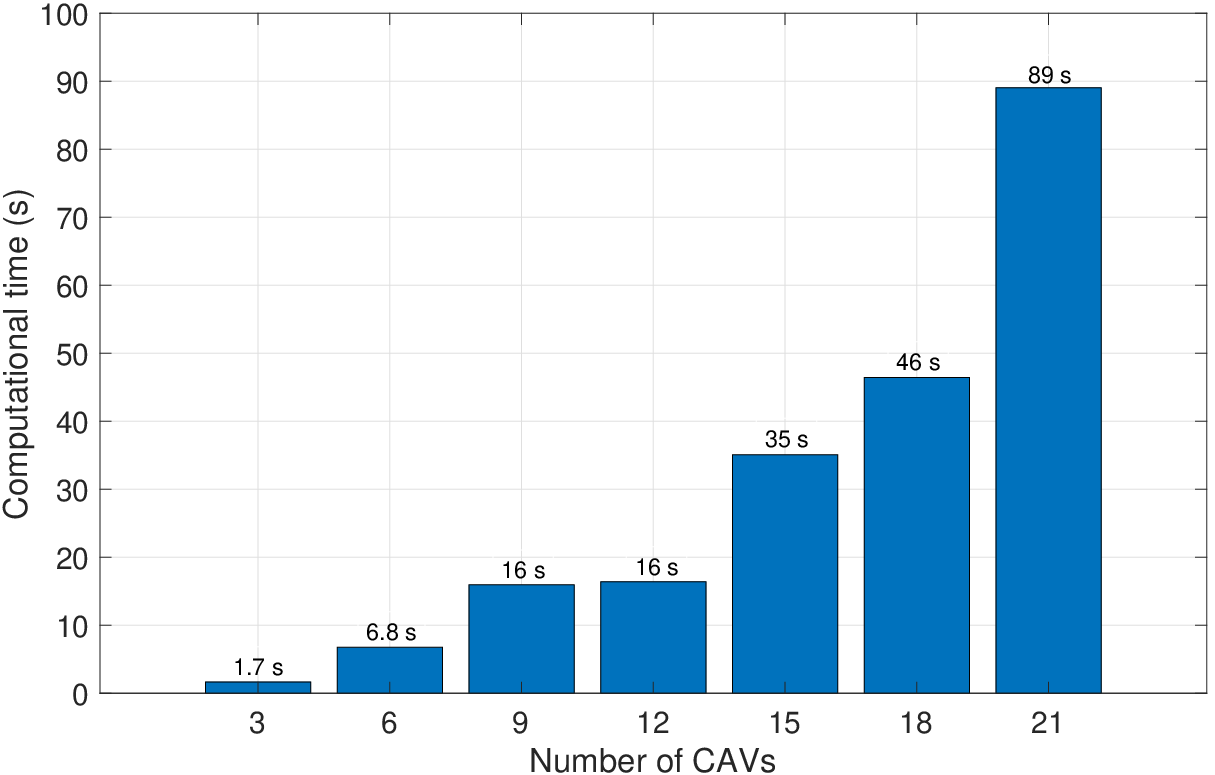
Fig. 4 depicts computational time of the proposed algorithm for different number of CAVs in test scenario two. The computation time of each number of CAV is the average of 10 times of running the scenario. The standard deviations of all the tests are less than $0.5\%$ which is negligible and are not shown. Fig. 4 shows that the computational complexity of the proposed algorithm is of the order of $O(e^{0.13n})$ in terms of number of CAVs $n$. The future work of this study is to reduce the computational time by decentralising the proposed strategy.

Fig 5(a) illustrates the total energy consumption of CAVs when the vehicles are controlled by the proposed and benchmark strategies in test scenario one. The figure also shows the total energy consumption of CAVs being controlled by the proposed strategy in test scenario two. The depicted graphs only consider the energy consumption due to acceleration which is calculated as follows:

where $E_{i}$ is the energy consumed by each $\text{CAV}_{i}$.

As seen in Fig. 5(a), the lane-free method proposed in [14] consumes the least energy, in cost of fixing the crossing time to an unnecessarily large value (i.e., 10 s). The proposed algorithm in this paper, in contrast, consumes more energy than both the benchmark strategies because it is optimised for minimisation of crossing time, as explained in section IV-A.

Moreover, the resulting energy consumption of this proposed strategy linearly increases with respect to the number of crossing CAVs in both the test scenarios. It can also be observed that CAVs consumes more energy in test scenario one than test scenario two because of a longer travelling distance due to diversity of destination of CAVs. Tables III and IV show the travelled distance of, respectively, test scenario one and two.

Fig. 5(b), on the other hand, compares the algorithms in terms of the energy consumption by each vehicle when travels one kilometer. As seen, all the strategies tend to consume less energy per vehicle per kilometer with an increase in the number of CAVs. This is due to the fact that the number of obstacles drops by reducing the number of crossing CAVs, and hence vehicles can accelerate and pass through faster in test scenario one.

To nullify energy consumption as one of the objectives, and only compare the crossing time of CAVs when they are controlled by the proposed strategy and the reservation-based one in [12], the acceleration gain $\gamma$ in (9) is tuned such that energy consumption of CAVs in both cases becomes the same. Table V shows the resulting performance of the proposed algorithm. As compared to the results of the reservation-based method in Table III, the proposed algorithm reduces the crossing time up to 52% (average of 40%) when consumes the same amount of energy. Moreover, whilst the average speed of CAVs is almost similar for both the strategies, the standard deviation of speed of CAVs controlled by the proposed algorithm is much lower. This indicates that CAVs controlled by the proposed algorithm travel with similar speed, whilst some of the CAVs being controlled by the reservation-based method travel with a much higher or lower speed than the others.

Fig. 6 depicts that the proposed algorithm finds the Pareto front of all the crossing solutions of 12 CAVs for different values of acceleration gain $\gamma$. As seen, the proposed strategy can achieve shorter crossing time than both the reservation-based method [12] and lane-free method [14] while consuming the same amount of energy. Moreover, the resulting crossing time of CAVs can be as close as possible to its theoretical lower bound.

Fig. 7 compares the calculate optimal speed and acceleration (or deceleration) trajectories by the proposed algorithm and reservation-based method in [12] for 12 CAVs in test scenario one, when energy consumption is the same.

As shown in Fig. 7(a), the maximum deceleration of CAVs when they are controlled by the proposed strategy is $1.4~m/s^{2}$ which is much less than the maximum permissible value of 3 $(m/s^{2})$. Moreover, the acceleration of all CAVs converges to zero at their destinations. Fig. 7(b), on the other hand, shows that some of the CAVs controlled by the reservation-based algorithm in [12] decelerate with the maximum permissible value, which is not converged to zero.

The maximum jerk of both algorithms is around 0.6 $m/s^{3}$, however, whilst jerks of CAVs controlled by the proposed strategy converges to zero, the passengers feel an uncomfortably constant jerk during the crossing time when CAVs are controlled by the reservation-based method in [12].

Fig. 7(c) as compared to Fig. 7(d) shows that all the vehicles travel within a much narrower range of speeds when they are controlled by the proposed algorithm. This means their passengers will experience similar feeling of speed, unlike the passengers of CAVs controlled by the reservation-based method in [12] who experience a diverged range of speeds (along with larger constantly applied jerk and higher acceleration/deceleration).

References

- [1] A. Foxx and P. John, “State transportation statistics,” in U.S. Department of Transportation, 2012.
- [2] J. Rios-Torres and A. A. Malikopoulos, “A survey on the coordination of connected and automated vehicles at intersections and merging at highway on-ramps,” IEEE Transactions on Intelligent Transportation Systems, vol. 18, no. 5, pp. 1066–1077, 2016.
- [3] Y. Zhang, A. A. Malikopoulos, and C. G. Cassandras, “Decentralized optimal control for connected automated vehicles at intersections including left and right turns,” in 2017 IEEE 56th Annual Conference on Decision and Control (CDC). IEEE, 2017, pp. 4428–4433.
- [4] P. Tallapragada and J. Cortés, “Hierarchical-distributed optimized coordination of intersection traffic,” IEEE Transactions on Intelligent Transportation Systems, vol. 21, no. 5, pp. 2100–2113, 2019.
- [5] B. Xu, S. E. Li, Y. Bian, S. Li, X. J. Ban, J. Wang, and K. Li, “Distributed conflict-free cooperation for multiple connected vehicles at unsignalized intersections,” Transportation Research Part C: Emerging Technologies, vol. 93, pp. 322–334, 2018.
- [6] M. Di Vaio, P. Falcone, R. Hult, A. Petrillo, A. Salvi, and S. Santini, “Design and experimental validation of a distributed interaction protocol for connected autonomous vehicles at a road intersection,” IEEE Transactions on Vehicular Technology, vol. 68, no. 10, pp. 9451–9465, 2019.
- [7] L. Makarem and D. Gillet, “Fluent coordination of autonomous vehicles at intersections,” in 2012 IEEE international conference on systems, man, and cybernetics (SMC). IEEE, 2012, pp. 2557–2562.
- [8] A. Mirheli, L. Hajibabai, and A. Hajbabaie, “Development of a signal-head-free intersection control logic in a fully connected and autonomous vehicle environment,” Transportation Research Part C: Emerging Technologies, vol. 92, pp. 412–425, 2018.
- [9] A. Mirheli, M. Tajalli, L. Hajibabai, and A. Hajbabaie, “A consensus-based distributed trajectory control in a signal-free intersection,” Transportation research part C: emerging technologies, vol. 100, pp. 161–176, 2019.
- [10] H. Xu, C. G. Cassandras, L. Li, and Y. Zhang, “Comparison of cooperative driving strategies for cavs at signal-free intersections,” IEEE Transactions on Intelligent Transportation Systems, 2021.
- [11] X. Pan, B. Chen, S. A. Evangelou, and S. Timotheou, “Optimal motion control for connected and automated electric vehicles at signal-free intersections,” in 2020 59th IEEE Conference on Decision and Control (CDC). IEEE, 2020, pp. 2831–2836.
- [12] A. A. Malikopoulos, L. Beaver, and I. V. Chremos, “Optimal time trajectory and coordination for connected and automated vehicles,” Automatica, vol. 125, p. 109469, 2021.
- [13] B. Li, Y. Zhang, Y. Zhang, N. Jia, and Y. Ge, “Near-optimal online motion planning of connected and automated vehicles at a signal-free and lane-free intersection,” in 2018 IEEE Intelligent Vehicles Symposium (IV). IEEE, 2018, pp. 1432–1437.
- [14] B. Li, Y. Zhang, N. Jia, and X. Peng, “Autonomous intersection management over continuous space: A microscopic and precise solution via computational optimal control,” IFAC-PapersOnLine, vol. 53, no. 2, pp. 17 071–17 076, 2020.
- [15] C. Liu, C.-W. Lin, S. Shiraishi, and M. Tomizuka, “Distributed conflict resolution for connected autonomous vehicles,” IEEE Transactions on Intelligent Vehicles, vol. 3, no. 1, pp. 18–29, 2017.
- [16] R. Hult, M. Zanon, S. Gros, and P. Falcone, “Optimal coordination of automated vehicles at intersections with turns,” in 2019 18th European Control Conference (ECC). IEEE, 2019, pp. 225–230.
- [17] R. Hult, M. Zanon, S. Gros, H. Wymeersch, and P. Falcone, “Optimisation-based coordination of connected, automated vehicles at intersections,” Vehicle System Dynamics, vol. 58, no. 5, pp. 726–747, 2020.
- [18] A. Katriniok, P. Kleibaum, and M. Joševski, “Distributed model predictive control for intersection automation using a parallelized optimization approach,” IFAC-PapersOnLine, vol. 50, no. 1, pp. 5940–5946, 2017.
- [19] M. Kloock, P. Scheffe, S. Marquardt, J. Maczijewski, B. Alrifaee, and S. Kowalewski, “Distributed model predictive intersection control of multiple vehicles,” in 2019 IEEE intelligent transportation systems conference (ITSC). IEEE, 2019, pp. 1735–1740.
- [20] A. A. Malikopoulos, C. G. Cassandras, and Y. J. Zhang, “A decentralized energy-optimal control framework for connected automated vehicles at signal-free intersections,” Automatica, vol. 93, pp. 244–256, 2018.
- [21] Y. Bian, S. E. Li, W. Ren, J. Wang, K. Li, and H. X. Liu, “Cooperation of multiple connected vehicles at unsignalized intersections: Distributed observation, optimization, and control,” IEEE Transactions on Industrial Electronics, vol. 67, no. 12, pp. 10 744–10 754, 2019.
- [22] A. Colombo and D. Del Vecchio, “Efficient algorithms for collision avoidance at intersections,” in Proceedings of the 15th ACM international conference on Hybrid Systems: Computation and Control, 2012, pp. 145–154.
- [23] D. Elliott, W. Keen, and L. Miao, “Recent advances in connected and automated vehicles,” journal of traffic and transportation engineering (English edition), vol. 6, no. 2, pp. 109–131, 2019.
- [24] W. Milliken and D. Milliken, Race Car Vehicle Dynamics, ser. Premiere Series. SAE International, 1995. [Online]. Available: https://books.google.co.uk/books?id=opgHfQzlnLEC
- [25] X. Zhang, A. Liniger, and F. Borrelli, “Optimization-based collision avoidance,” IEEE Transactions on Control Systems Technology, vol. 29, no. 3, pp. 972–983, 2021.
- [26] S. Boyd and L. Vandenberghe, Convex Optimization. Cambridge University Press, 2004.
- [27] R. Firoozi, L. Ferranti, X. Zhang, S. Nejadnik, and F. Borrelli, “A distributed multi-robot coordination algorithm for navigation in tight environments,” arXiv preprint arXiv:2006.11492, 2020.
- [28] J. A. E. Andersson, J. Gillis, G. Horn, J. B. Rawlings, and M. Diehl, “CasADi – A software framework for nonlinear optimization and optimal control,” Mathematical Programming Computation, vol. 11, no. 1, pp. 1–36, 2019.
- [29] A. Wächter and L. T. Biegler, “On the implementation of an interior-point filter line-search algorithm for large-scale nonlinear programming,” Mathematical programming, vol. 106, no. 1, pp. 25–57, 2006.
- [30] C. Rösmann, A. Makarow, and T. Bertram, “Time-optimal control with direct collocation and variable discretization,” arXiv preprint arXiv:2005.12136, 2020.