Identifying Ambiguous Similarity Conditions via Semantic Matching
Abstract
Rich semantics inside an image result in its ambiguous relationship with others, i.e., two images could be similar in one condition but dissimilar in another. Given triplets like “aircraft” is similar to “bird” than “train”, Weakly Supervised Conditional Similarity Learning (WS-CSL) learns multiple embeddings to match semantic conditions without explicit condition labels such as “can fly”. However, similarity relationships in a triplet are uncertain except providing a condition. For example, the previous comparison becomes invalid once the conditional label changes to “is vehicle”. To this end, we introduce a novel evaluation criterion by predicting the comparison’s correctness after assigning the learned embeddings to their optimal conditions, which measures how much WS-CSL could cover latent semantics as the supervised model. Furthermore, we propose the Distance Induced Semantic COndition VERification Network (DiscoverNet), which characterizes the instance-instance and triplets-condition relations in a “decompose-and-fuse” manner. To make the learned embeddings cover all semantics, DiscoverNet utilizes a set module or an additional regularizer over the correspondence between a triplet and a condition. DiscoverNet achieves state-of-the-art performance on benchmarks like UT-Zappos-50k and Celeb-A w.r.t. different criteria.
1 Introduction
Learning embeddings (a.k.a. representations) from data benefits machine learning and visual recognition systems davis-et-al-icml-2007; weinberger09distance; amid2015MVTE; Schroff2015FaceNet; Ye2016What; feng2020uncertainty; Opitz2020Deep; Ye2020Learning; zhou2022forward. Side information such as triplets Song2016Deep; Sohn2016Improved; Manmatha2017Sampling; Elezi2020Group; Duan2020Deep indicates the comparison relationship of objects, from which the embedding pulls visually similar objects close while pushing dissimilar ones away.
The linkage between objects conveys rich information about the object itself as well as its relationship with others, which becomes ambiguous when the similarity is measured from different perspectives. As illustrated in Fig. 1 (upper), (a) female with glasses, (b) female without glasses, and (c) male with glasses are organized in triplets.11 1 In a valid triplet , is more similar than . We think (a) and (b) are more similar when we measure based on “gender”. In contrast, we also treat (a) and (c) as neighbors since they “wear glasses”. Since one embedding space outputs fixed relationships between instances, learning multiple embeddings facilitates discovering rich semantics.


Given triplets associated with their condition labels, indicating under what kind of similarity the comparisons are made, Conditional Similarity Learning (CSL) learns multiple embeddings to cover latent semantic Veit2017Conditional; Wang2017Contextual. During the evaluation, CSL predicts whether a triplet is meaningful or not under a specified condition. Although supervised CSL has been successfully applied in various applications Lee2018Stacked; Plummer2018Conditional; Vasileva2018Learning; Lin2020Fashion, labeling conditions introduces additional costs. As in a recommendation system, users may click relevant items (label item-wise similarities) based on particular preferences, and we only collect diverse comparison relationships without explicit condition labels. Tan2019Learning; Nigam2019Towards propose Weakly Supervised-CSL (WS-CSL), where multiple embeddings are learned with triplets and the model is unaware of their corresponding conditions.
Current WS-CSL borrows the evaluation protocol from supervised CSL Veit2017Conditional, which checks the validness of a triplet but neglects the specified condition. For example, we predict whether “aircraft” is similar to “bird” than “train” conditioned on “can fly” in the supervised scenario, but ask the model to predict the correctness of the triplet free from the condition in WS-CSL. Since a triplet could be ambiguous, WS-CSL may focus on weighting those embeddings to explain the triplet instead of learning semantically conditional embeddings corresponding to the ground-truth.
We demonstrate the challenge with the following experiment. After removing all condition labels of correct triplets, we compute the proportion a WS-CSL model predicts those triplets as valid ones via its learned embeddings, which equals the “accuracy” used in WS-CSL evaluation. Then we reverse those triplets — changing the order of the second and the third items, which makes them invalid under previous conditions. We further compute the valid ratio over reversed triplets. Results in Fig. 1 (lower left) show an optimal supervised model has 100% and 0% proportion/accuracy in two cases. A WS-CSL method SCE-Net Tan2019Learning has a higher proportion than the supervised CSN Veit2017Conditional on original triplets as well as a high proportion on reversed ones, which means it treats both original and reversed triplets as valid. The diverse results between WS-CSL and its supervised counterparts indicate the “accuracy” is biased towards predicting all triplets as valid, and the correctness of a triplet without a specified condition is meaningless. To check the coverage of all semantics, we propose to measure the comparison ability of multiple learned embeddings after assigning them to target conditions.
We also propose Distance Induced Semantic COndition VERification Network (DiscoverNet) to balance the ability of comparison prediction and semantic coverage. DiscoverNet works in a “decompose-and-fuse” manner, which identifies similarity conditions and captures the ambiguous relationship with discriminative embeddings.
We aim to ensure the learned multiple embeddings in WS-CSL are able to reveal the similarities in the target conditions as much as the supervised methods. In DiscoverNet, we achieve the goal from two aspects. First, we use a set module to map various triplets with the same set of instances to one condition, avoiding messy training update signals. On the other hand, we add a regularizer to force selecting different conditional embeddings when a model predicts both a triplet and its reversed one as valid. DiscoverNet demonstrates higher performance on benchmarks like UT-Zappos-50k in our newly proposed criterion, which is shown in Fig. 1 (lower right). The code is available at https://github.com/shiy19/DiscoverNet.
Our contributions could be summarized as:
- •
We point out the challenges in WS-CSL evaluation and design a novel criterion.
- •
Based on the proposed DiscoverNet, we improve the quality of learned embeddings and match the ground-truth semantics from two aspects.
- •
DiscoverNet can identify latent rich conditions and works better than others in our criterion.
2 Related Work
Metric Learning. Learning embeddings from data attracts lots of attention in machine learning and computer vision. The learned embeddings encode the relationship between objects well and facilitate downstream tasks chechik2010large; Schroff2015FaceNet; Song2016Deep; Hsieh2017Collaborative. With the guidance of the comparison relationship between object pairs davis-et-al-icml-2007, triplets weinberger09distance; Ye2020Learning, and higher-order statistics law2016learning, visually similar instances are pulled together, and visually dissimilar ones are pushed away. Types of loss functions are proposed Bell2015Learning; Song2016Deep; Song2017Deep; Opitz2020Deep; Manmatha2017Sampling; Elezi2020Group; Duan2020Deep to take full advantage of the similarity comparisons between instances in a mini-batch, e.g., the triplet loss Schroff2015FaceNet and N-Pair loss Sohn2016Improved.
Conditional Similarity Learning (CSL). Different from measuring all linkages with a single metric, the relationship between objects could be measured from diverse aspects (under different conditions) Memisevic2004Multiple; Maaten2012Visualizing; NIPS2013_SCA. In Veit2017Conditional; Yu2017Semantic, CSL is investigated by associating conditions with image attributes, and multiple diverse embeddings could be derived from feature masks to capture the semantic of various conditions. CSL has been applied in applications like image-text classification Liu2019Neural; Nigam2019Towards, fashion retrieval Tan2019Learning; Hou2021Learning; Dong2021Fine, zero-shot learning Zhang2015Zero and video grounding Shi2019Not. Condition labels during training link a particular embedding with a condition, and the learned embeddings are evaluated by predicting the validness of a triplet under a certain condition.
Weakly supervised CSL. Explicit condition labels are unavailable in some cases, e.g., we get a comparison tuple once a user selects an item than others without any knowledge of his/her preference (condition). The weakly supervised CSL, i.e., learning conditional embeddings without condition annotations is investigated in amid2015MVTE, where a model infers conditions given a triplet and then decides the right embedding to use for training and deployment. Tan2019Learning emphasizes the comparison ability of the fused embedding, while Ye2016What; Nigam2019Towards select one metric from multiple candidates to explain a triplet. Using the same evaluation protocols as CSL, weakly supervised CSL can get higher performance than supervised CSL without involving the ground-truth condition labels. We analyze the protocol and point out its drawbacks of semantic coverage. We propose a new criterion to reveal the difference between the quality of the learned embedding and its supervised counterpart. We also propose DiscoverNet to trade-off the diversified embedding and semantic fusion in a “decompose and fuse” manner. A set module and a semantic regularizer are discussed to make DiscoverNet cover all target conditions.
3 Notations and Background
We organize comparisons into triplets, i.e., . For three items in : the anchor has a similar target neighbor , and an impostor is dissimilar with . Similarity in could be determined by categories of instances. The embedding, a.k.a., feature extractor, projects an instance into a latent space, whose distance with is
| (1) |
is a projection. We implement with deep neural network, and learn embedding by minimizing the violation of comparisons over triplets. Define the validness of a triplet by comparing the distances between “anchor-impostor” and “anchor-target neighbor”, i.e.,
| (2) |
If the anchor has a larger distance with the impostor than with the target neighbor, the embedding is consistent with the relationship in . Given a loss , e.g., the margin loss or the logistic loss, we optimize . Then would be larger than the margin , so that anchor and the target neighbor are pulled while the impostor would be pushed away.
Conditional similarity learning (CSL).
Comparisons in triplet may vary across environments. For example, when we ask which image in a candidate set is close to a given anchor, different workers may measure the similarities from their own aspects. In CSL, we associate a condition label with each triplet, i.e., , indicating based on the -th condition the comparison in is made. One embedding fails to capture the diverse relationship when comparisons with the same set of instances are opposite, e.g., vs. . CSL extends , , and to , , and , respectively. embeddings covering conditions are optimized:
| (3) |
outputs 1 when the input is true and 0 otherwise. In Eq. 3, only the distance corresponding to condition of the triplet is activated. In evaluation, is used to check whether a triplet from the -th condition is valid or not.
Weakly supervised CSL (WS-CSL).
Due to additional annotation costs and ambiguity of condition labels, the triplet-wise condition labels are unknown in WS-CSL. The model needs to infer condition labels and activates the corresponding embeddings to capture triplet’s characteristic. The target of WS-CSL is to learn a set of embeddings , which is able to capture those semantics of target conditions as much as the supervised CSL.
4 Evaluation of Weakly Supervised CSL
Current WS-CSL follows CSL to measure by predicting whether three instances could form a triplet without a condition label. We analyze the issues of the current criterion and propose our new evaluation protocol.

4.1 Analysis of Supervised CSL Evaluation
In supervised CSL evaluation, a model is asked to determine whether a triplet is valid or not given the condition . In detail, we get with the corresponding conditional embedding and predict as valid if . Since and could not co-exist, we sample the same number of valid triplets from each condition in evaluation. The average accuracy (proportion of triplets predicted as correct) over them reveals the quality of a CSL model.
Since the ability of comparison prediction is important, previous WS-CSL methods follow this protocol without using the test-time condition labels. In other words, we predict whether a triplet is correct without its condition label. So in this case, a WS-CSL model predicts the validness of a triplet with all learned embeddings.
There are two issues when evaluating with the supervised protocol directly. First, a model tends to find a condition to explain the triplet, which predicts all triplets as true in most cases, e.g., even for reversed triplets (demonstrated in Fig. 1). Specifically, given a valid , we construct , and ask a WS-CSL model whether is valid or not. Since is invalid under the same condition , an optimal supervised model will predict as true and as false. However, a WS-CSL method SCE-Net Tan2019Learning predicts most original () and reversed () triplets as valid, which makes the evaluation biased.
Moreover, the current evaluation predicts the validness of the triplet while neglecting from which condition the WS-CSL model determines the relationship. We’d like a WS-CSL model works similarly to a supervised one, so not only the fusion of conditional embeddings should cover all target semantics, but also the behavior of each reveals the relationship w.r.t. a specific condition. Therefore, we propose a new criterion to meet the previous requirements.
4.2 Condition Alignment for WS-CSL Evaluation
We claim that predicting the validness of a triplet is only meaningful given a specific condition. Based on the ground-truth conditions and the validness of triplets during the evaluation, we propose a two-step new criterion. First, we map target conditions to WS-CSL embeddings . Then, we evaluate triplets accuracy with corresponding as in the supervised scenario, which reveals how much a WS-CSL model covers the target conditions as the supervised model.
We assume there is the same number of embeddings and conditions.22 2 Our analysis could be extended when their numbers do not match. Given triplets from the -th condition for evaluation, we compute the triplet prediction accuracy with . We collect accuracy for all conditions and form a cost matrix , whose element is the error (100 minus the accuracy) using -th embedding to predict the triplets from the -th condition. The alignment could be obtained from with the following two strategies.
Greedy Alignment. We use a greedy strategy to find the most suitable embedding, i.e., , for a condition . So one embedding may handle multiple conditions.
OT Alignment. We optimize the following Optimal Transport (OT) objective villani2008optimal to obtain a mapping from the embedding set to the condition set
| (4) |
Eq. 4 minimizes the total cost when we use an embedding to predict triplets from another condition. We set the marginal distribution of the transportation as uniform. By minimizing Eq. 4 we obtain as a map. Element reveals how much the -th embedding is related to the -th condition. We can further obtain a one-to-one mapping based on under assumptions Courty2017Optimal. Fig. 2 shows a comparison between our proposed and previous criteria.
Discussions. Based on our criterion, a WS-CSL model gets high accuracy only when all conditions can be explained with certain learned embeddings, and the model predicts triplets from diverse aspects well with different embeddings. Thus our criterion depicts the “semantic coverage” of , which also reveals the gap between in WS-CSL and its supervised counterpart. We may compute the cost over the validation data with a small amount of ground-truth condition labels, and use the obtained alignment to compute the final accuracy on the test set. Benefiting from this condition-embedding alignment, our criterion naturally avoids the issue from the reversed triplets shown in Fig. 1.
5 DiscoverNet for Weakly-Supervised CSL
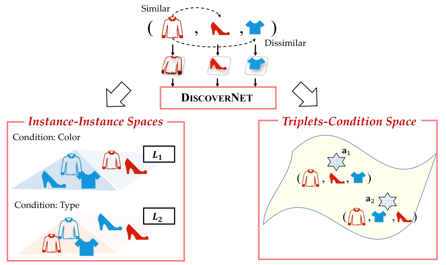
We’d like to learn the embedding set to cover all rich semantics, and the comparison relationship under each target condition could be revealed by a certain conditional embedding . We propose Distance Induced Semantic Condition VERification Network (DiscoverNet) for WS-CSL (illustrated in Fig. 3). DiscoverNet introduces a “triplets-condition” space to match condition scores of a triplet, which automatically selects or fuses multiple pairwise distances measured by “instance-instance” spaces. As we discussed before, a WS-CSL model could violate the semantic constraints over artificially reversed triplets, which influences the coverage of semantics. We consider a set module to avoid those cases during training, which maps various triplets with the same set of instances to one condition. Furthermore, we add a regularizer to force the model to select diverse conditions if both original and reversed triplets are predicted as valid ones.
5.1 Decompose and Fuse Hierarchical Spaces
We assume condition-specific embeddings have different projections but share the same .33 3 Since conditions are not independent, it is not necessary to match each condition with an embedding . More discussions are in experiments. Then we have
| (5) |
The space measured by projection biases towards a “local” view of the embedding , and allows inconsistent comparisons across different “instance-instance” spaces.
The overall linkages between objects are measured based on a fused distance over condition-specific comparisons. Different from the indicator in Eq. 3 selecting the distance, we use a multinomial distributed variable to denote the latent condition label of a triplet . There are binary elements in . We optimize and jointly:
| (6) |
The condition of the triplet is revealed by the expected distance w.r.t. the distribution of Ye2017Learning, which selects or fuses the related conditions of the triplet. If a triplet could only be valid under the -th condition, we expect has the -th element and other elements equal 0. Then the expected distance activates the -th metric, and the target neighbor (resp. impostor) is pulled close (resp. pushed away) with . The -th embedding becomes more specific for the condition. If the triplet is related to more conditions, we expect to fuse the semantics from multiple distances together. Therefore, values in determine whether to select or fuse conditional embeddings, which emphasizes the semantic coverage or comparison prediction, respectively.
Given , the variable indicates the influence of the posterior probability that a triplet belongs to the -th condition. We introduce a “triplets-condition” space, where a triplet is embedded to a point with mapping . summarizes the triplet and maps the set of embeddings in into a -dimensional vector. We expect triplets with similar conditions will be close. Furthermore, learnable anchors captures those similarity conditions, and we match a triplet to its closest anchor:
| (7) |
We implement the similarity with cosine. is the temperature. The larger the , the more uniform is. If a triplet is related to the -th condition, then its transformed vector is close to the anchor . Then a larger emphasizes the -th condition when computing the expected distance. Benefited from the “decompose and fuse” manner in Eq. 7, a triplet that has a clear condition tendency will be close to a particular anchor, which makes becomes one-hot, and the embedding is highly correlated with the corresponding condition. Then embeddings will cover more semantics. Those ambiguous triplets will have a nearly uniform . Although hard to differentiate semantics in this case, their fused distances take advantage of all embeddings to predict the validness of triplets and improve the comparison prediction ability.
Instance Space for Semantic Discovery. Given , we define the -th conditional embedding as
| (8) |
We obtain the local embedding in a residual form, where encodes the similarity bias of the -th condition based on the general embedding . If is discriminative enough for a particular similarity condition, we do not need to over-allocate the local metric. In other words, strong makes degenerate to zero. In summary, distances for different similarity conditions in Eq. 5 are calculated based on .
5.2 Condition Space for Semantic Fusion
Based on our analyses in Section 4, a WS-CSL model could violate the semantic constraints in vanilla training. A too flexible mapping will make the model treat both a triplet and its reversed version as correct ones while activating almost the same conditional embedding . In other words, the model may focus on fusing those conditions with and collapse all semantics into one conditional space.
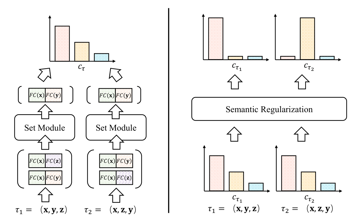
Since semantic constraints on a WS-CSL model are limited, we address the issue with the help of artificially reversed triplets. For a pair of original triplet and its reversed version, we restrict the model’s flexibility by either weakening the representation ability of with a set module or adding another semantic regularizer (illustrated in Fig. 4).
Set Module. A natural way to implement is to capture the order of instances in a triplet with a sequential model Hochreiter1997Long; Tan2019Learning. As we mentioned, a triplet and its reversed version should belong to different conditions. However, without any constraints, we find a sequential module has the ability to weight conditions in different manners for and , but it is likely to work in a “lazy” way. In detail, a model may learn a strong conditional embedding and map both and to similar distributions that have larger weights on and small weights on others. Then, rather than making learned embeddings associated with corresponding conditional semantic meanings, a model tends to improve the fusion module and use partial embeddings to cover all semantics.
Therefore, we consider a set module to make agnostic with the order in the triplet. In particular, we use the pairwise concatenation of instance embeddings as the input of , i.e., for a triplet , we obtain its embeddings, and get the augmented set:
which encodes the pairs in . Since is not included in , we get the same representation for and the reversed . Moreover, to take a holistic view of , we transform with element-wise maximization Zaheer2017Deepsets:
| (9) |
is a fully connected network with one hidden layer and ReLU activation, which projects the given input to a same-dimensional output. With Eq. 9, the pairwise relationship in the triplet is evaluated first, and the most evident one is activated to represent the whole triplet. In summary, the set module restricts the ability of and makes one triplet and its reversed version have the same representation. Although it is a bit counter-intuitive, the special configuration of avoids the ambiguous update directions of the model so that the conditional embeddings should be more discriminative to cover the target semantics. We also investigate the Transformer Vaswani2017Attention implementation of in the supplementary.
Semantic Regularizer. We can also think from another aspect by regularizing a representative . We set Eq. 9 to
covering the sequential information of instances. Due to an additional pair in , different orders of instances in and do not share the same output. In this case, it is abnormal when the model predicts and based on the same condition . We construct a semantic regularization to avoid this case. If and (the model treats two triplets as valid ones),44 4 We check this condition with the current model during training. Parameters in here are detached without gradient back propagation. we add the following semantic regularizer to make the activated conditions diverse:
| (10) |
In other words, if and are predicted as valid ones, we minimize the similarity between their condition distributions and . The similarity between these two multinomial distributions are measured with Histogram Intersection Kernel (HIK) Grauman2005The; Wu2010Fast; Wu2013C4, which is the sum of element-wise minimum of two distributions. Therefore, with the help of Eq. 10, we explicitly enforce the WS-CSL model considers different conditional embeddings to explain triplets, which further improve the semantic coverage of .
Discussions. There are two implementations of DiscoverNet, using the set module or the semantic regularizer. The two strategies are designed from different aspects to make the WS-CSL model contain rich semantics as much as the supervised model. Since the set module avoids the diverse selection for reversed triplet naturally, it satisfies the regularizer directly. Thus, it does not help if we combine two strategies together.
6 Experiments
We verify the effectiveness of DiscoverNet over benchmarks based on our new criterion. Ablation studies and visualization results demonstrate DiscoverNet learns conditions successfully as the supervised methods. Detailed setups and more results are in the supplementary.
6.1 Experimental Setups
Datasets. UT-Zappos-50k Shoes contains 50,025 images of shoes with four similarity conditions collected online Yu2014finegrained; Yu2017Semantic. Following Veit2017Conditional; Tan2019Learning; Nigam2019Towards, we discretize the “height” condition and resize all images to 112 by 112. There are 200,000, 20,000, and 40,000 triplets following splits in Veit2017Conditional for training, validation and test, respectively. Celeb-A Faces has 202,599 face images of different identities Liu2015Deep. 8 of the 40 attributes (conditions) are selected for analysis Nigam2019Towards. We resize all images to 112 by 112. 400,000/80,000/160,000 triplets are used for model training/validation/test. We construct a more difficult Celeb-A† by combining related binary attributes in Celeb-A together, where each multi-choice condition has 5-7 discrete values, We apply the same configuration for Celeb-A variants.
Splits. All models are trained and evaluated over triplets in Veit2017Conditional. Since there are no published triplets over Celeb-A, we randomly sample triplets by ourselves. Equal number of triplets for each attribute are sampled from the standard training, validation, and test split of Celeb-A Liu2015Deep. For each triplet, we organize instances with the same attribute label into a similar pair. Otherwise, we think they are dissimilar.
Criterion. We utilize our proposed new criterion to evaluate WS-CSL methods. After constructing a mapping from condition to learned embeddings with greedy or OT strategies, we compute the average triplet prediction accuracy as in the supervised case. We denote the results with two strategies as GR Accuracy and OT Accuracy, respectively.
Comparison Methods. We compare DiscoverNet with both supervised method Conditional Similarity Networks (CSN) Veit2017Conditional and two WS-CSL methods, i.e., Latent Similarity Networks (LSN) Nigam2019Towards and Similarity Condition Embedding Network (SCE-Net) Tan2019Learning.
Implementation Details. Following Veit2017Conditional; Nigam2019Towards; Tan2019Learning, we use ResNet-18 He2016Residual to implement . Different from previous literature fine-tuning the backbone based on the weights pre-trained on ImageNet Deng2009Imagenet, we also consider the case that we train the full model from scratch. The model with the best accuracy over the validation set is selected for the final test.
6.2 Benchmark Evaluations
| Setups | w/ pretrain | w/o pretrain | ||
|---|---|---|---|---|
| Criteria | GR Acc. | OT Acc. | GR Acc. | OT Acc. |
| CSN Veit2017Conditional | 87.86 | 87.86 | 82.14 | 82.14 |
| LSN Nigam2019Towards | 76.26 | 75.90 | 71.49 | 68.49 |
| SCE-Net Tan2019Learning | 72.21 | 71.15 | 64.08 | 61.03 |
| DiscoverNetSet | 76.98 | 75.68 | 74.67 | 74.13 |
| DiscoverNetReg | 77.84 | 77.68 | 72.99 | 71.46 |
UT-Zappos-50k. The results of DiscoverNet and comparison methods over UT-Zappos-50k are listed in Table 1, which contains the greedy accuracy and OT accuracy over both pre-trained and non-pre-trained weights. We re-implement all comparison methods. DiscoverNetSet and DiscoverNetReg denote the variant using set module and semantic regularization, respectively.
By observing both setups and criteria, CSN becomes the “upper-bound” for WS-CSL methods. The main reason is that ground-truth condition labels in CSN associate an embedding with a particular condition during training. The supervised CSN gets the same greedy and OT accuracy. The explicit supervision in CSN makes those embeddings biased towards different semantics, which gets the same one-to-one OT mapping with the greedy strategy. WS-CSL methods get lower OT accuracy than the corresponding greedy accuracy. The main reason is that OT accuracy requires a one-to-one mapping between embeddings and conditions, where those conditions would be related. While greedy accuracy allows one embedding to handle multiple conditions.
As we discussed before, SCE-Net tends to fuse the semantic meaning of embeddings with its self-attention module, so each of its learned embeddings is hard to cover a specific condition. By contrast, LSN performs better in our criteria, benefiting from its multi-choice learning paradigm. Our DiscoverNet can get the best performance among WS-CSL methods. In detail, DiscoverNetSet works better when training from scratch and DiscoverNetReg performs well with the pre-trained weights. One possible reason is that the pre-trained weights are strong and make the model (especially the mapping function ) too flexible, so an explicit regularization helps more. In summary, our criterion reveals how much similar a WS-CSL model performs to a supervised one.

(a) Functional Types

(b) Closing Mechanism

(c) Suggested Gender

(d) Height of Heels
| Celeb-A | Celeb-A† | |||
| Criteria | GR Acc. | OT Acc. | GR Acc. | OT Acc. |
| CSN Veit2017Conditional | 83.41 | 83.41 | 67.72 | 67.72 |
| LSN Nigam2019Towards | 70.29 | 69.89 | 57.02 | 56.33 |
| SCE-Net Tan2019Learning | 69.47 | 51.81 | 51.49 | 50.64 |
| DiscoverNetSet | 78.45 | 77.98 | 64.57 | 63.98 |
| DiscoverNetReg | 78.04 | 76.96 | 57.43 | 56.94 |
Celeb-A. In Table 2, we investigate (the 8 attribute) Celeb-A and its variant Celeb-A† with model trained from scratch. DiscoverNetSet and DiscoverNetReg still get better performance than other WS-CSL counterparts, while CSN is still the ‘upper bound’ due to the help of condition labels.
6.3 Ablation Studies and Visualizations
We analyze the properties of DiscoverNet and show the visualization results. More analysis such as the help of the WS-CSL embeddings given limited conditional supervisions are in the supplementary.
| DiscoverNetSet | DiscoverNetReg | |||
|---|---|---|---|---|
| # Projections | GR Acc. | OT Acc. | GR Acc. | OT Acc. |
| 2 | 78.28 | 77.74 | 71.92 | 71.82 |
| 4 | 79.58 | 77.60 | 73.19 | 71.32 |
| 6 | 80.41 | 77.69 | 75.53 | 73.87 |
| 8 | 80.65 | 78.81 | 75.19 | 74.07 |
| 10 | 81.35 | 78.68 | 76.09 | 73.77 |

(a) 5 o Clock Shadow

(b) Eyeglasses

(c) Male

(d) Wearing Lipstick
Influence of condition number configuration. We set the number of embeddings in benchmarks the same as the number of ground-truth conditions, which is 8 in Celeb-A. We show the change of the two criteria along with the increase of the embedding number in Table 3. Both DiscoverNetSet and DiscoverNetReg get higher OT accuracy when the number of embeddings increases from two to eight, and decreases from eight to ten. We conjecture that allocating too many local metrics interfere with each other and their related semantics partially overlap. Besides, greedy accuracy shows a generally incremental trend since it allows one embedding to handle multiple conditions.
Visualization of semantic embeddings. To better illustrate how our DiscoverNet learns for different semantics, we provide TSNE visualizations for each of the learned semantic spaces on UT-Zappos-50k in Fig. 5. DiscoverNet captures the variety of conditions and learns different embeddings for the dataset with good interpretability. Typically, on the condition “height of heels”, the heel height of the shoes is decreasing from the left-top of the embedding space to the bottom, then to the right-top.
Visualization of conditional image retrieval. We provide image-retrieval visualizations for four conditions on Celeb-A in Fig. 6. We keep the anchor image, and retrieve its neighbor from a set of randomly collected candidates with different local embeddings. Benefiting from the correspondence obtained when computing the OT accuracy, we can qualitatively measure whether a local embedding could reveal the corresponding semantic via its ranking of images. For example, on the “Male” condition, since the anchor image has the label “Female”, DiscoverNet makes all images labeled “Female” close while pushing images related to “Male” away. The results indicate our DiscoverNet can cover latent semantics of data and each of its learned conditional embedding corresponds to a particular meaningful semantic.
7 Conclusion
We revisit WS-CSL and observe that evaluating the quality of the model without specifying concrete conditions produces biased accuracy. Thus, we match multiple learned embeddings with ground-truth conditions in advance before predicting the correctness of given triplets, which simultaneously considers the ability of triplet prediction and semantic coverage. We also utilize a set module or a semantic regularizer in our proposed DiscoverNet to emphasize the correspondence between a conditional embedding and a semantic condition. DiscoverNet outperforms other WS-CSL methods on benchmarks with different criteria.
Limitations. Our new criterion evaluates WS-CSL in a “supervised” manner by assigning multiple learned embeddings to target conditions. The criterion does not fit the case when the goal is not to learn a model similar to its supervised counterpart, e.g., to distinguish whether triplets are correct and explain their validness as much as possible.
Acknowledgments. This research was supported by National Key R&D Program of China (2020AAA0109401), NSFC (62006112, 61921006, 62176117), Collaborative Innovation Center of Novel Software Technology and Industrialization, NSF of Jiangsu Province (BK20200313).
References
- (1) Ehsan Amid and Antti Ukkonen. Multiview triplet embedding: Learning attributes in multiple maps. In ICML, pages 1472–1480, 2015.
- (2) Sean Bell and Kavita Bala. Learning visual similarity for product design with convolutional neural networks. ACM Transactions on Graphics, 34(4):98:1–98:10, 2015.
- (3) Soravit Changpinyo, Kuan Liu, and Fei Sha. Similarity component analysis. In NIPS, pages 1511–1519, 2013.
- (4) Gal Chechik, Varun Sharma, Uri Shalit, and Samy Bengio. Large scale online learning of image similarity through ranking. JMLR, 11:1109–1135, 2010.
- (5) Nicolas Courty, Rémi Flamary, Devis Tuia, and Alain Rakotomamonjy. Optimal transport for domain adaptation. TPAMI, 39(9):1853–1865, 2017.
- (6) Jason V. Davis, Brian Kulis, Prateek Jain, Suvrit Sra, and Inderjit S. Dhillon. Information-theoretic metric learning. In ICML, pages 209–216, 2007.
- (7) Jia Deng, Wei Dong, Richard Socher, Li-Jia Li, Kai Li, and Fei-Fei Li. Imagenet: A large-scale hierarchical image database. In CVPR, pages 248–255, 2009.
- (8) Jianfeng Dong, Zhe Ma, Xiaofeng Mao, Xun Yang, Yuan He, Richang Hong, and Shouling Ji. Fine-grained fashion similarity prediction by attribute-specific embedding learning. CoRR, abs/2104.02429, 2021.
- (9) Yueqi Duan, Jiwen Lu, Wenzhao Zheng, and Jie Zhou. Deep adversarial metric learning. TIP, 29:2037–2051, 2020.
- (10) Ismail Elezi, Sebastiano Vascon, Alessandro Torcinovich, Marcello Pelillo, and Laura Leal-Taixé. The group loss for deep metric learning. In ECCV, pages 277–294, 2020.
- (11) Boyuan Feng, Yuke Wang, Zheng Wang, and Yufei Ding. Uncertainty-aware attention graph neural network for defending adversarial attacks. CoRR, abs/2009.10235, 2020.
- (12) Kristen Grauman and Trevor Darrell. The pyramid match kernel: Discriminative classification with sets of image features. In ICCV, pages 1458–1465, 2005.
- (13) Kaiming He, Xiangyu Zhang, Shaoqing Ren, and Jian Sun. Deep residual learning for image recognition. In CVPR, pages 770–778, 2016.
- (14) Sepp Hochreiter and Jürgen Schmidhuber. Long short-term memory. Neural Computation, 9(8):1735–1780, 1997.
- (15) Yuxin Hou, Eleonora Vig, Michael Donoser, and Loris Bazzani. Learning attribute-driven disentangled representations for interactive fashion retrieval. In ICCV, pages 12147–12157, 2021.
- (16) Cheng-Kang Hsieh, Longqi Yang, Yin Cui, Tsung-Yi Lin, Serge J. Belongie, and Deborah Estrin. Collaborative metric learning. In WWW, pages 193–201, 2017.
- (17) Marc T Law, Nicolas Thome, and Matthieu Cord. Learning a distance metric from relative comparisons between quadruplets of images. IJCV, pages 1–30, 2016.
- (18) Kuang-Huei Lee, Xi Chen, Gang Hua, Houdong Hu, and Xiaodong He. Stacked cross attention for image-text matching. In ECCV, pages 212–228, 2018.
- (19) Yen-Liang Lin, Son Tran, and Larry S. Davis. Fashion outfit complementary item retrieval. In CVPR, pages 3308–3316, 2020.
- (20) Weiyang Liu, Zhen Liu, James M. Rehg, and Le Song. Neural similarity learning. In NeurIPS, pages 5026–5037, 2019.
- (21) Ziwei Liu, Ping Luo, Xiaogang Wang, and Xiaoou Tang. Deep learning face attributes in the wild. In ICCV, pages 3730–3738, 2015.
- (22) R. Manmatha, Chao-Yuan Wu, Alexander J. Smola, and Philipp Krähenbühl. Sampling matters in deep embedding learning. In ICCV, pages 2859–2867, 2017.
- (23) Roland Memisevic and Geoffrey E. Hinton. Multiple relational embedding. In NIPS, pages 913–920, 2004.
- (24) Ishan Nigam, Pavel Tokmakov, and Deva Ramanan. Towards latent attribute discovery from triplet similarities. In ICCV, pages 402–410, 2019.
- (25) Michael Opitz, Georg Waltner, Horst Possegger, and Horst Bischof. Deep metric learning with BIER: boosting independent embeddings robustly. TPAMI, 42(2):276–290, 2020.
- (26) Bryan A. Plummer, Paige Kordas, M. Hadi Kiapour, Shuai Zheng, Robinson Piramuthu, and Svetlana Lazebnik. Conditional image-text embedding networks. In ECCV, pages 258–274, 2018.
- (27) Florian Schroff, Dmitry Kalenichenko, and James Philbin. Facenet: A unified embedding for face recognition and clustering. In CVPR, pages 815–823, 2015.
- (28) Jing Shi, Jia Xu, Boqing Gong, and Chenliang Xu. Not all frames are equal: Weakly-supervised video grounding with contextual similarity and visual clustering losses. In CVPR, pages 10444–10452, 2019.
- (29) Kihyuk Sohn. Improved deep metric learning with multi-class n-pair loss objective. In NIPS, pages 1849–1857, 2016.
- (30) Hyun Oh Song, Stefanie Jegelka, Vivek Rathod, and Kevin Murphy. Deep metric learning via facility location. In CVPR, pages 2206–2214, 2017.
- (31) Hyun Oh Song, Yu Xiang, Stefanie Jegelka, and Silvio Savarese. Deep metric learning via lifted structured feature embedding. In CVPR, pages 4004–4012, 2016.
- (32) Reuben Tan, Mariya I. Vasileva, Kate Saenko, and Bryan A. Plummer. Learning similarity conditions without explicit supervision. In ICCV, pages 10373–10382, 2019.
- (33) Laurens van der Maaten and Geoffrey E. Hinton. Visualizing non-metric similarities in multiple maps. Machine Learning, 87(1):33–55, 2012.
- (34) Mariya I. Vasileva, Bryan A. Plummer, Krishna Dusad, Shreya Rajpal, Ranjitha Kumar, and David A. Forsyth. Learning type-aware embeddings for fashion compatibility. In ECCV, pages 405–421, 2018.
- (35) Ashish Vaswani, Noam Shazeer, Niki Parmar, Jakob Uszkoreit, Llion Jones, Aidan N. Gomez, Lukasz Kaiser, and Illia Polosukhin. Attention is all you need. In NIPS, pages 5998–6008, 2017.
- (36) Andreas Veit, Serge J. Belongie, and Theofanis Karaletsos. Conditional similarity networks. In CVPR, pages 1781–1789, 2017.
- (37) Cédric Villani. Optimal transport: old and new, volume 338. Springer Science & Business Media, 2008.
- (38) Xiaofang Wang, Kris M. Kitani, and Martial Hebert. Contextual visual similarity. CoRR, abs/1612.02534, 2016.
- (39) Kilian Q. Weinberger and Lawrence K. Saul. Distance metric learning for large margin nearest neighbor classification. JMLR, 10:207–244, 2009.
- (40) Jianxin Wu. A fast dual method for HIK SVM learning. In ECCV, pages 552–565, 2010.
- (41) Jianxin Wu, Nini Liu, Christopher Geyer, and James M. Rehg. ${\rm C}ˆ{4}$: A real-time object detection framework. TIP, 22(10):4096–4107, 2013.
- (42) Han-Jia Ye, De-Chuan Zhan, Yuan Jiang, and Zhi-Hua Zhou. What makes objects similar: A unified multi-metric learning approach. TPAMI, 41(5):1257–1270, 2019.
- (43) Han-Jia Ye, De-Chuan Zhan, Nan Li, and Yuan Jiang. Learning multiple local metrics: Global consideration helps. TPAMI, 42(7):1698–1712, 2020.
- (44) Han-Jia Ye, De-Chuan Zhan, Xue-Min Si, and Yuan Jiang. Learning mahalanobis distance metric: Considering instance disturbance helps. In IJCAI, pages 3315–3321, 2017.
- (45) Aron Yu and Kristen Grauman. Fine-grained visual comparisons with local learning. In CVPR, pages 192–199, Jun 2014.
- (46) Aron Yu and Kristen Grauman. Semantic jitter: Dense supervision for visual comparisons via synthetic images. In ICCV, pages 5571–5580, 2017.
- (47) Manzil Zaheer, Satwik Kottur, Siamak Ravanbakhsh, Barnabás Póczos, Ruslan Salakhutdinov, and Alexander J. Smola. Deep sets. In NIPS, pages 3391–3401, 2017.
- (48) Ziming Zhang and Venkatesh Saligrama. Zero-shot learning via semantic similarity embedding. In ICCV, pages 4166–4174, 2015.
- (49) Da-Wei Zhou, Fu-Yun Wang, Han-Jia Ye, Liang Ma, Shiliang Pu, and De-Chuan Zhan. Forward compatible few-shot class-incremental learning. In CVPR, 2022.