reception date \Acceptedacception date \Publishedpublication date \SetRunningHeadAstronomical Society of JapanUsage of pasj00.cls
Black hole physics—Hydrodynamics— Accretion, accretion disks– Galaxies: active—galaxies: jets
Dragged surfaces. On the accretion tori in the ergoregion
Abstract
We discuss the conditions for the existence of extended matter configurations orbiting in the ergoregion or close to the outer ergosurface of the Kerr black hole (”dragged” configurations). The corotating tori under consideration are perfect fluid configurations with barotropic equation of state, orbiting on the equatorial plane of the central Kerr black hole. The possibility of magnetized tori with a toroidal magnetic field is also discussed. Indications on the attractors where dragged tori can be observed are provided with the analysis of the fluid characteristics and geometrical features, relevant for the tori stability and their observations. QPOs emissions from the inner edges of the dragged tori are also discussed. We argue that the smaller dragged tori could be subjected to a characteristic instability, effect of the frame-dragging. This possibility is thoroughly explored. This can finally lead to the destruction of the torus (disk exfoliation) which can combine with accretion and processes present in the regions very close to the black hole horizon. Tori are characterized according to the central attractor dimensionless spin. These structures can be observed orbiting black holes with dimensionless spin .
1 Introduction
Although restricted by the typical assumptions of the simplified models, geometrically thick (stationary) disks provide a striking good approximation of several aspects of accretion in more complex dynamical models, some of these features include indication on tori location, the disk elongation on their symmetry plane, the inner edge of quiescent and accreting disks, the tori thickness, the maximum height, and the critical pressure points in the disks. In this article we explore accreting toroidal matter orbiting a central Kerr black hole (BH), within the hydrodynamic model introduced and detailed in a series of works (Paczyński&Wiita 1980; Paczyński 1980; Kozłowski et al. 1978; Abramowicz et al. 1996; Fishbone&Moncrief 1976; Frank et al. 2002; Pugliese et al. 2013; Pugliese&Montani 2015).
This is a fully general relativistic model of an opaque and super-Eddington, pressure supported disk, cooled by advection based on the Boyer theory of the equilibrium and rigidity in general relativity (Boyer 1965). In the Boyer model, many features of the disk dynamics and morphology like the disk thickness, the disk stretching on the equatorial plane and the disk location, are predominantly constrained by the geometric properties of spacetime via an effective potential function regulating the pressure gradients in the Euler equation. The effective potential function contains two main components: a dynamical term, related to the orbiting matter by means of the fluid angular momentum, here assumed constant along the disk, and a geometrical one related to the properties of the spacetime background. The boundary of any stationary, barotropic, perfect fluid torus is determined by the equipotential surface, which are the surfaces of constant pressure, defined by the gradient of a scalar function, i.e. the effective potential. This property holds if, for barotropic fluids, the relativistic frequency turns to be function of the fluid angular momentum only or (von Zeipel conditions) (Kozłowski et al. 1978; Abramowicz 1971; Chakrabarti 1991; Chakrabarti 1990). Accretion onto the attractor is driven through the vicinity of the cusp (corresponding to the inner edge of the cusped toroid) in the self crossed (cusped) closed configurations from a violation of the hydrostatic equilibrium, i.e., due to Paczyński mechanism (Kozłowski et al. 1978; Paczyński&Wiita 1980; Paczyński 1980). This mechanism has been proved to be also an important stabilizing mechanism against the thermal and viscous instabilities locally, and against the so called Papaloizou&Pringle instability (PPI) globally (Blaes 1987; Abramowicz&Fragile 2013; Paczyński 1980; Paczyński&Wiita 1980; Kozłowski et al. 1978). During the evolution of dynamical processes, the functional form of the angular momentum and entropy distribution depends on the initial conditions of the system and on the details of the dissipative processes.
We focus on tori orbiting in regions close to the BH static limit and in the BH ergoregion, which is the region between the outer ergosurface and the (outer) event horizon, defining the partially contained and dragged surfaces. (The outer ergosurface is also called stationary limit surface or static limit, for the absence of any (timelike) static observers inside the region). A partially contained torus is centered (location of maximum pressure point) in the outer region, but a part of the torus inner region, which is bounded from the below by the inner edge and from the above by the torus center, orbits in the ergoregion.
Thick accretion disks are usually associated with very compact objects like black holes and super massive BHs (SMBHs). Directly involved in the equilibrium phases of the attractors, they are very likely the base of the jet formation and dynamics, the Active Galactic Nuclei (AGN) and Gamma Ray Bursts (GRBs) emissions. In this context the dynamics inside the ergoregion is extremely relevant in Astrophysics: accreting matter can support, for example, jets of matter or radiation originated inside the ergoregion (Meier 2012; Gariel et al. 2013), which can empower jets with powerful Poynting flux, as from ergospheric disks studied in Punsly 2007.
The processes occurring inside the BH ergoregion are essential for understanding the central engine mechanism of many emissions (Meier 2012; Frolov&Zelnikov 2011). The mechanism, by which energy from compact spinning objects is extracted, is of great astrophysical interest: BH rotational energy can be extracted through the classical Penrose process, and indeed the super-radiance as seen by asymptotic observers. Black hole thermodynamics has been grounded on the observation that the BH energy can actually be extracted from the black hole, and ergoregion is the background geometrical engine of many processes of energy extraction from the Kerr BH. The ergosurface is also the geometric basic of super-radiant scattering of incident waves which is the wave analog of the Penrose process, based on the fact that the particles energy, within the ergoregion, as measured by an observer at infinity, can also be negative11 1 The presence of negative energy particles is also a distinctive feature of the ergoregion in weakly rotating naked singularities (WNS) differentiating these from the BHs. (The superirradiance and ergoregion instability is a further characteristic differentiating BHs from NSs.). The static limit can act as a semi-permeable membrane separating the spacetime region, filled with negative energy particles from the external one, filled with positive. The WNSs ergoregion is characterized by the existence of zero and negative energy states circular orbits (stable circular geodesics with negative energy)(Stuchlík 1980; Stuchlík& Schee 2012; Charbulák&Stuchlík 2018; Stuchlík et al 2018). The presence of this special matter in an “antigravity” sphere, possibly filled with negative energy matter formed according to the Penrose process, and bounded by orbits with zero angular momentum, could have an important role in the source evolution(Hawking&Ellis 1973; Penrose&Floyd 1971). (BH super-radiance also appears to distinguish bosonic waves from the fermions in the super-radiant amplification).
The rotational energy can be extracted from the source, lowering its angular momentum. The Penrose energy extraction, and the super-radiance are classical phenomena due to the frame-dragging of the spinning spacetime. Another possibility is the extraction of energy from a rotating black hole through the Blandford-Znajek mechanism (Blandford&Znajek 1977; Pei et al. 2016; Komissarov 2009; Lasota et al. 2014; Penrose 1969) and magnetic Penrose process or radiative Penrose process(Kološ et al. 2021; Tursunov et al. 2020). The Hawking radiation instead arises from the vacuum fluctuations in the regions close to the BH horizon, it is the spontaneous emission of thermal radiation which is created in the vacuum regions surrounding a BH, and it may eventually lead to a decrease of the BH mass (Penrose&Floyd 1971; Hawking 1976; Hawking 1971; Bekenstein 1975).
In this article we characterize the orbiting extended matter configurations orbiting in the ergoregion of a Kerr BH, introducing the concept of dragged tori and partially contended tori made by corotating perfect fluids thick tori. We discuss possible instabilities by exploring the effects of geometry frame-dragging on the disk exfoliation and evaluating the pressure gradients which are the main factor for the tori formation and formation of a possible atmosphere of (free) particles swarm. A possible outcome of the instabilities of the smallest tori could be an emission of swarm of particles and photons, enhanced accretion, or the torus destruction. Dragged and partially contained tori are also subjected to processes typical of the regions very close to the black hole horizon as, for example, the Runaway Instability. To evaluate this situation, we asses the torus verticality, the dragged torus geometrical thickness, the influence of the dragging frame on the disk thickness, and the location of the tori extreme of pressure with the respect to the static limit. We proceed to the exploration of the tori characteristics in dependence on the central attractor dimensionless spin, providing eventually indications on the attractors where dragged tori can be observed. Some extreme configurations in the ergoregion are also described, as proto-jets which are open cusped General Relativistic Hydrodynamic (GRHD) configurations, limiting solutions for the thick disks models, and the possibility of orbiting agglomerates of toroids composed by an aggregate of multi toroids orbiting in the ergoregion.
In the second part of this work, dragged and partially contained tori are studied in relation to the quasi-periodic oscillations (QPOs) in emission from the tori inner edges. We relate also the dragged tori in the ergoregion and the maximum extractable rotational energy from the BH horizon, constituting the state prior the total extraction of the energy from the BH, following the approach introduced in Daly 2009, which is quite independent from the details of the specific process of energy extraction, and based on the definition of BH irriducible mass function, rotational energy and using the BH classical thermodynamical law. (The energy extraction through the accretion process, the rotational energy converted into radiation corresponds to the binding energy of the fluid). For large part of this analysis we shall consider perfect fluids defined by a barotropic equation of state; however, we also investigate the possibility that the frame dragging could differentiate different polytropics. In this context we provide an estimation of the the flux thickness, mass-flux and enthalpy-flux for dragged and partially contained thick disks with a fixed polytropic fluid.
The article is organized as follows: In Sec. (2) we introduce the thick accretion model and the fluid effective potential for the toroidal configurations in a Kerr spacetime background. Dragged surfaces and partially contended tori are introduced in Sec. (3.1). In Sec. (3.1.1) the tori verticality is studies and disk exfoliation is introduced. Dragged disks thickness is the focus of Sec. (3.1.2) where the influence of the dragging frame on the disk thickness is investigated. In Sec. (3.1.3) we explore the process of tori exfoliation. Extreme configurations as orbiting agglomerates of toroids and proto-jets are briefly considered in Sec. (3.1.4). Characteristic frequencies of the oscillations of the toroids are studied in Sec. (3.2) and in Sec. (3.2.1) where we discuss the origin of the QPOs emission in relations to the toroids in the ergoregion. Analysis of possible polytropic fluids for dragged and partially contained tori is in Sec. (3.3). Discussion on some aspects of tori energetics for these tori is in Sec. (3.3.1). Conclusions are Sec. (4). In Appendix (A) there are some notes on stationary magnetized tori in the ergoregion.
2 Fluid configuration on the Kerr spacetime
We consider a perfect fluid orbiting in the Kerr spacetime background, where the metric tensor can be written in Boyer-Lindquist (BL) coordinates as follows
| (1) | |||
where and are the lapse function and the frequency of the zero angular momentum fiducial observer (ZAMOS) (Pugliese&Quevedo 2018), whose four velocity is , being orthogonal to the surface of constant . here is a mass parameter and the specific angular momentum is given as , where is the total angular momentum of the gravitational source and , . In the following it will be also convenient to introduce the quantity . We will consider the Kerr black hole (BH) case defined by , the extreme black hole source , and the non-rotating limiting case of the Schwarzschild metric. The horizons and the static (or stationary) limit are respectively
| (2) |
where on the planes and it is i on the equatorial plane . In the region (ergoregion or outer ergoregion), there is (time component of the metric tensor) and -Boyer-Lindquist coordinate becomes spacelike, this fact implies that a static observer cannot exist inside the ergoregion. The radius is the ergosurface, or, precisely, outer ergosurface. In this work we investigate toroidal configurations of perfect fluid orbiting a Kerr SMBH, it will be therefore convenient to consider first the properties of the test particle circular motion. Since the metric is independent of and , the covariant component of a particle four–momentum, and , are conserved along the geodesics or22 2 We adopt the geometrical units and the signature, Latin indices run in . The four-velocity satisfy . The radius has unit of mass , and the angular momentum units of , the velocities and with and . For the seek of convenience, we always consider the dimensionless energy and effective potential and an angular momentum per unit of mass .
| (3) | |||
| (4) |
The momentum of the particle with mass and four-velocity can be normalized so that , where for null, spacelike and timelike curves, respectively. Quantities are constants of motion for circular test particles geodesics where is the Killing field representing the stationarity of the Kerr geometry and is the axial Killing field; the vector is spacelike in the ergoregion. In general, we may interpret , for timelike geodesics, as representing the total energy of the test particle coming from radial infinity, as measured by a static observer at infinity, and as the axial component of the angular momentum of the particle. The normalization condition on the four-velocity can be solved for the energy . For circular motion there is . Considering the motion on the fixed equatorial plane , no motion is in the angular direction and (the Kerr metric is symmetric under reflection through the equatorial plane ). Within these assumptions we obtain the effective potential : circular orbits are therefore described by
| (5) |
Some notable radii regulate the particle dynamics, namely the marginal circular orbit for timelike particles, which is also a photon orbit, the marginal bounded orbit at , and the marginal stable circular orbit at with angular momentum and energy respectively, where is for counterrotating or corotating orbits with respect to the attractor. It is convenient to introduce also the relativistic angular frequency and the specific angular momentum as follows
| (6) | |||
We consider a one-specie particle perfect fluid (simple fluid), where
| (7) |
is the fluid energy momentum tensor, and are the total energy density and pressure, respectively, as measured by an observer moving with the fluid. For the symmetries of the problem, we always assume and , being a generic spacetime tensor (we can refer to this assumption as the condition of ideal hydrodynamics of equilibrium). The timelike flow vector field denotes now the fluid four-velocity. The motion of the fluid is described by the continuity equation and the Euler equation respectively:
| (8) |
where the projection tensor (from the conservation equation along the tensor defined by the fluid, where .). We investigate in particular the case of a fluid circular configuration, defined by the constraint . Tori are centered on the central BH, orbiting on its equatorial plane which is also the tori symmetry plane–see for example Figs (1). On the fixed plane , no motion is assumed in the angular direction, which means . We assume moreover a barotropic equation of state . The continuity equation is identically satisfied as consequence of these conditions. From the Euler equation (8) we obtain
| (9) |
The function is Paczynski-Wiita (P-W) potential, function is the torus (fluid) effective potential 33 3 We can relate the fluid effective potential with the test particles circular orbits potential as where and and where , here , and is related to the norm of stationary observers whose frequency is and is defined in Eq. (4). Light surfaces have . Note, that the effective potential of the fluids and the particles, as defined here in the hydrostatic model, is related to the constant energy of the test particle motion and . These quantities could be negative in the ergoregion. The presence of (geodetical) circular motion with or in the ergoregion is a well known feature of the Kerr naked singularity solutions which has also zamos, zero angular momentum, observers, which has not equivalent in the ergoregion of the BH and it is a distinctive feature of certain naked singularities with ”small” spin–mass ratios. This characteristic has been attributed to the repulsive gravity effects of the NSs. We also note that this feature is capable to define an effective ergoregion in the field of Reissner-Norström geometry (electrically charged and static metric). In the case we consider here circular orbit has and therefore effective potential is always positive. (The energy may be negative as measured at infinity, locally it is always positive.) (Stuchlík&Schee 2013; Stuchlík& Schee 2012) Here we specify that (not well defined) in some circumstances inside the ergoreigon, it is related to the normalization conditions on the fluid 4-momentum which is stationary (i.e. the associated fluid four momentum has , where is the relativistic angular velocity which satisfies to the von Zeipel conditions) therefore well defined in the ergoregion. There is for and [ () with with which is a photon orbit in the ergoregion., reflecting the background Kerr geometry and the centrifugal effects through the fluid specific angular momentum . The fluid equilibrium is therefore regulated by the balance of the gravitational and pressure terms versus centrifugal factors arising due to the fluid rotation and the curvature effects of the Kerr background, encoded in the effective potential function . Here and, for large part of this analysis, we shall consider mainly the radial gradients of pressure.


Assuming the fluid is characterized by the specific angular momentum constant across the torus (see also Lei et al. 2008; Abramowicz&Fragile 2013), we consider, from Eq. (9) the critical points of the pressure in the torus as the extremes of the effective potentials considering the solutions constant, introducing therefore the couple of tori parameters . The toroidal surface are equipressure surfaces, therefore equipotential surfaces with constant, for a given constant 44 4 This fully general relativistic model of pressure supported torus, traces back to the Boyer theory of the equilibrium and rigidity in general relativity, i.e. the analytic theory of equilibrium configurations of rotating perfect fluids (Boyer 1965; Frank et al. 2002). Each toroid is governed by the General Relativity hydrodynamic condition of equilibrium configurations of rotating perfect fluids applied to toroidal surfaces.These correspond also to the surfaces of constant density , specific angular momentum , and constant relativistic angular frequency , where as a consequence of the von Zeipel theorem (Chakrabarti 1990; Chakrabarti 1991; Zanotti&Pugliese 2015). In this model the entropy is constant along the flow and the rotation law is independent of the equation of state (Abramowicz&Fragile 2013). In these tori in fact the functional form of the angular momentum and entropy distribution during the evolution of dynamical processes, could be considered as dependent only on the initial conditions of the system see Abramowicz&Fragile 2013. In this situation the surfaces of constant enthalpy, pressure and density coincide with the surfaces of constant effective potential , fixed by the integration parameter related to the boundary conditions on the integration of the Euler equation. The torus surfaces are surfaces of constant pressure or constant for , (Frank et al. 2002), where it is indeed and for .–(Abramowicz&Fragile 2013; Pugliese&Montani 2015; Pugliese&Stuchlík 2015; Pugliese et al. 2013) and for example Abramowicz 1971; Abramowicz 1985; Abramowicz et al. 1996; Adamek&Stuchlík 2013; Fishbone&Moncrief 1976; Font&Daigne 2002; Frank et al. 2002; Komissarov 2006; Lei et al. 2008; Montero et al. 2007; Pugliese&Montani 2013; Pugliese&Montani 2018; Pugliese&Stuchlík 2016; Pugliese&Stuchlík 2017; Pugliese&Stuchlík 2018a; Pugliese&Stuchlík 2018b; Pugliese&Stuchlík 2019; Pugliese&Stuchlík 2021; Zanotti&Pugliese 2015.
According to Eq. (9), tori centers (maximum pressure points) and cusps (minimum pressure points), are the critical points of as function of the radius . The maximum of the hydrostatic pressure corresponds to the minimum of the effective potential , and it is the torus center . The instability points of the tori (P-W mechanics), are located at the minima of the pressure, correspondent to the maximum of as functions of –see Figs (1).
More generally, equation can be solved for the fluid specific angular momentum obtaining the function ”leading function”. We also introduce the function (”energy function”) which, as function , is also dependent on the BH dimensionless spin, and are defined as:
| (10) |
for counterrotating and corotating fluids respectively. Functions and are showed in connection with the tori surfaces in Figs (1). Functions define the hydrostatic pressure critical points in the torus, centers of maximum pressure or cusps . Curves locate the tori centers and provide information on torus elongation and density and, for a torus accreting onto the central BH, determine the inner, , and outer, , torus edges, where the elongation on the equatorial plane is –Figs (1) and Figs (2). The couple of constant parameters uniquely identifies each toroidal surface and these can be directly reduced to a single parameter , in presence of a cusp. (The critical points of the pressure are determined by the parameter only, therefore in the case of cusped tori, the cusp fixes uniquely also the -parameter, coincident with the maximum value of the torus effective potential–Figs (1)).
More specifically, solutions of the problem constant lead to three classes of configurations corresponding to ––cross sections of the closed surfaces (equilibrium quiescent torus); –cross sections of the closed cusped surfaces (accreting torus)– –cross sections of the open cusped surfaces, generally associated to proto-jet configurations.
The closed, not cusped, surfaces are associated to stationary equilibrium (quiescent) toroidal configurations. For the cusped and closed equipotential surfaces, , the accretion onto the central black hole can occur through the cusp of the equipotential surface. In this situation the outflow of matter through the cusp occurs as the torus surface exceeds the critical equipotential surface (having a cusp), leading to a mechanical non-equilibrium process, i.e. an instability in the balance of the gravitational and inertial forces and the pressure gradients, where matter inflows into the central black hole (a violation of the hydrostatic equilibrium known as Paczyński mechanism). In the case considered here the accreting flow ”starts” across a ”Lagrange point” (Roche lobe overflow, due to Paczynski accretion mechanics (Paczyński 1980; Paczyński&Wiita 1980). This is the cusp of the orbiting toroidal surface, which is an important aspect of thick disks since its presence also stabilizes the tori against several instabilities (thermal and viscous local instabilities, and globally against the Papaloizou-Pringle instability-PPI and it could be possibly connected to QPOs emission.) (Abramowicz&Fragile 2013).
Therefore, in this accretion model we shortly indicate the cusp of the self-crossed closed toroidal surface as the ”inner edge of accreting torus”. Finally, the open equipotential surfaces, which are briefly considered in Sec. (3.1.4), have been associated to the formation of proto-jets (Pugliese&Stuchlík 2016; Pugliese&Stuchlík 2018c; Pugliese&Stuchlík 2018b).
The minimum points of the hydrostatic pressure are constrained by the geodesic structure of the Kerr geometry. Alongside the geodesic structure of the Kerr spacetime, we include radii solution of , and radii and or more generally , regulating the maximum points of the pressure, and defined as the solutions of the following equations
| (11) | |||
| (12) |
respectively for the counterrotating and corotating orbits–Figs (3).


Radii , and constitute the extended geodetic structure of the spacetime. (Location of radii with respect to the radii Eqs (12) depend on the BH spin).
We summarize the constraints, defining ranges of fluids specific angular momentum defining the closed quiescent, cusped or open configurations and the tori location (cusp and tori centers) with respect to the central BH:
- –Tori
-
For there are quiescent and cusped tori, with topologies ; accretion point is and center with maximum pressure is ;
- –Tori
-
For there are quiescent tori and proto-jets, with topologies ; unstable point is on and center with maximum pressure ;
- –Tori
-
For there are quiescent tori with center , holding respectively for corotating and counterrotating tori,
Let be function evaluated at and respectively. Closed, not cusped configurations are for where according to the momentum or respectively, cusped configurations are for –see Figs (3). As we study the configurations inside the ergoregion, we consider mainly corotating fluids, therefore notation to indicate the corotating tori will be generally omitted. For any quantity evaluated on a general radius , we adopt notation We also adopt the notation or for any quantity relative to the cusped torus . Where appropriate, to easy the reading of complex expressions, we will use the geometric units where and .
3 In the outer ergoregion
Here we characterize the orbiting tori in the outer ergoregion or close to the static limit. In section (3.1) we introduce the concept of dragged surfaces and partially contained surfaces which are analyzed in Sec. (3.1.1) particularly with the investigation of the the tori verticality and introducing the disk exfoliation for dragged tori. The influence of the dragging frame on the disk thickness is the focus of Sec. (3.1.2), while in Sec. (3.1.3) we deepen the discussion on the tori exfoliation. We conclude this section in Sec. (3.1.4), with some notes on limiting configurations as the possibility of multi-tori (aggregates of multi-toroids) in the ergoregion, the proto-jets and tori.
3.1 Dragged surfaces
We explore two types of closed configurations in :
- (1)
-
The closed quiescent configurations ;
- (2)
-
The closed tori with cusps , having specific angular momentum .
In Sec. (3.1.4) we consider also the proto-jets, open toroidal configurations, in the ergoregion.
As discussed in Pugliese&Montani 2015, we can consider an evolutive parameter following the configurations evolution, from the phase of disk formation, assuming a simplified two-phase accretion tori evolution, to the accretion phase. Naturally one can consider the parameter evolution with a negative ”time-gradient”, where decreasing in region , with the consequent evolution of to and to with an ”over-critical” toroid where there is formation of an accretion throat, corresponding to the torus cusp enlargement and associated to matter flowing– Figs (1). Cusped tori are considered limiting configurations for the accretion phases. The disk may also be subsequently stabilized (in quiescent tori) to a sequence of interrupted phases of super-Eddington accretion as often considered in models of SMBHs evolution (Volonteri et al. 2007; Volonteri 2007; Volonteri 2010; Volonteri et al. 2003; Li 2012; Oka et al. 2017; Kawakatu&Ohsuga 2011; Allen et al. 2006), occurring, for example, in composed systems of tori aggregates as the eRAD (Pugliese&Stuchlík 2015; Pugliese&Stuchlík 2017; Pugliese&Stuchlík 2019). A further possibility consists in the formation of an accretion throat, for over critical tori, with , and formation of a fat torus with accretion material very close to the horizon.
We focus specifically on the following two types of configurations:
- 1. Dragged surfaces
-
Dragged surfaces are closed quiescent, , or closed cusped tori entirely contained in the ergoregion. This definition considers the tori radial dimension, i.e., we assume the torus inner, , and outer edge , be both located in the range . This condition however does not imply the torus entire containment in at any plane . Considering the disk vertical dimension, tori defined by constant fixed may cross the ergosurface at a plane , including the tori geometrical maximum which is related to the maximum pressure point. We focus the analysis of the disks verticality in considering the ergosurface crossing at any in Figs (14,15,16,17,18) and Sec. (3.1.1).
- 2. Partially contained configurations
-
The partially contained tori are characterized by the conditions and . This case has the following two sub-cases, which can also be associated to different phases of the tori evolution inside the ergoregion: (a) In the first sub-class of partially contained tori, the disk inner part, region , is fully contained in the ergoregion, which may include also a section the torus outer part, . (b) In the second sub-class of tori, only a section of the torus inner part is contained in the ergoregion (that is a region with . This condition implies that the projection on the equatorial plane of the maximum geometrical point is out of the ergoregion. (In the following we consider, when not otherwise stated, the projection of the geometrical maximum of the surface on the equatorial plane.).
The tori stability in is an important issue to be assessed, that can involve a series of hypothesis on the dragged and partially contained surfaces formation. Tori evolution may develop from a configuration formed outside the ergoregion, then evolving in partially contained and from partially contained to dragged surfaces, featuring, therefore, disk formation in three stages. This hypothesis can be grounded on the assessment of appropriate details of disk formation, as growing from accreting matter from the embedding, and conditions on the accretion process, for example in the case where the central SMBH is a part of a binary system having an accreting companion star. A second possibility consists in the formation of a torus in the ergoregion crossing the ergosuface from the outer part of the torus. (Note that there is , therefore there is a first phase when crosses the ergosurface, implying also the torus crossing the ergosurface on planes different from the equatorial plane). Finally, a third hypothesis features a disk formed inside the ergoregion, growing in the ergoregion and accreting into the central attractor. The problem of disk approaching and crossing the static limit or the formation of the closed quiescent torus across the static limit is also faced by the analysis of the disk vertical dimension, rephrasing the problem for a torus crossing the ergoregion on different planes. Following the torus growing, and the accreting disk stretching on the equatorial plane, the torus outer edge may cross the static limit, leading the initial dragged surface to a subsequent partially contained configuration. It may be possible that the dragged configurations could appear as seeds, formed in-loco, on a range centered on the orbit . This situations can be also largely affected by the details of fluids characteristics as the equations of state or differentiated in more complicated frames as the GRMHD models, we consider this issue briefly in Sec. (3.3) and Appendix (A). (However as we note from the Euler equation in the GRHD model, the ”pressure-forces” are entirely regulated by the fluid effective potential gradient, and possibly the fluid relativistic angular velocity and the gradient of the specific angular momentum for model with constant, while it is independent from the details of the polytropics).
The disks embedding is another relevant aspect of the dragged configurations, i.e., tori could be formed following accretion in a binary system or they can result also as the consequence, for instance, of the Bardeen–Petterson effect on an originally misaligned torus, broken due to the frame dragging and other factors, as the fluids viscosity, in an inner corotating torus and an outer torus which may also be counter-rotating (Bardeen&Petterson 1975; Nealon et al. 2015). A second possibility can also consider the Bardeen-Petterson effect on an original, partially contained, torus-(Nealon et al. 2015; Martin et al. 2014; King&Nixon 2018; Nixon et al. 2012a; Nixon et al. 2012b; Nealon et al. 2015; Lodato&Pringle 2006; Scheuerl&Feiler 1996; King et al. 2005). Vertical stresses in the disks, and the polar gradient of pressure, can combine with the Lense-Thirring effect. Consequentially, a relevant issue of these processes for the stability of the partially contained configurations, is whether the inner or outer part of the disk is in the ergoregion and, the case of crossing of the outer ergosurface on planes different from the equatorial plane, which may affect the torus (global) stability when stretching towards the horizon during accretion. For this reason we consider more in details the torus inner and outer edges location with respect to the static limit.
- –The inner edge
-
The inner edge of tori with specific angular momentum in satisfies the relation with . For any dragged or partially contained configuration, we concentrate on the problem of penetration of the inner edge of the tori in the outer ergoregion, assuming firstly , and considering cusped tori . A necessary but not sufficient condition for partially contained or dragged surfaces, is the occurrence of , distinguishing therefore two classes of BH attractors, which we consider more in details in Figs (2). The value is a limiting condition for configurations approaching the ergoregion, being very close to the outer ergosurface. Condition is a sufficient but not necessary condition for a partially contained torus (a section of the torus inner part being contained). It is clear that the necessary but not sufficient condition for the torus to be centered in the ergoregion, i.e. the maximum pressure point would be inside the ergoregion, is that . A sufficient but not necessary condition for the torus center to be included in the ergoregion is . The analysis of the limiting situation is faced in Figs (4) solving the equivalent problem for a given spacetime , where .


Figure 4: Notable radii of the spacetime geometry. Dashed curve is the radius , radius is the outer ergosurface, showing the inner edge of the disk whose center is in or viceversa the center of the disk whose cusp is in . Black curve is the outer edge of the accreting torus . Black region is the BH horizon. Marginally bounded orbit is , blue curve as is radius , red curve is marginally stable orbit , orange curve is the photon orbit , where radius is also represented as orange curve. Panels show different ranges of the BH dimensionless spin . (We note that the center of maximum pressure and the minimum pressure point in the torus are determined by the specific angular momentum only, while the geometrical maximum is regulated by the parameter once fixed ). The torus cusp may also be in the near-horizon region for very high spins of the central SMBH (partially contained for and entirely contained for ). (For we intend the minimum points of the pressure , which can be a cusp of the closed torus or the cusp of a proto-jet ). Analysis of the inner edge location with respect to the static limit is in Figs (10) and (9).
- –The outer edge
-
If , the condition is possible for some and values. The condition is necessary but not sufficient condition for the outer edge of a configuration to be included in the ergoregion. The inner part of such tori can be in part . The inner part of a configuration must be in the ergoregion. The condition is necessary but not sufficient condition for the outer edge of a configuration to be included in the ergoregion. The inner part of such tori can be in part in . The inner part of a configuration must be in the ergoregion. Analysis of the outer edge location with the respect to the static limit is in Figs (6,7,8,22).
The maximum elongation of the dragged torus is at most . The surfaces with very large specific angular momentum , , tend to be stable against the cusp formation, leading to quiescent closed configurations. An interesting question is whether these configurations, stabilized by a large centrifugal component (the cusp absence), are dragged or partially contained toroidal surfaces rather then tori with lower specific angular momentum characterized with the cusp formation or the quiescent configurations with 55 5 This issue is indeed relevant for the stability of these configurations as the relativistic Roche lobe overflow at the cusp of the equipotential surfaces is also the stabilizing mechanism against the thermal and viscous instabilities locally, and against the so called Papaloizou–Pringle instability globally (Blaes 1987). (For a discussion on the relation between Papaloizou-Pringle (PP) global incompressible modes in the tori, the Papaloizou-Pringle Instability (PPI), a global, hydrodynamic, non-axi-symmetric instability and the Magneto-Rotational Instability (MRI) modes see Pugliese&Montani 2018; Bugli et al. 2018).. These configurations can also grow very huge, with the center of maximum pressure in the torus at for large spin .
In Figs 3 we show the regions of tori parameters for the existence of the closed tori, featuring also the possibility of double cusped configurations for BHs with high-spin, while in Figs (5) curves constant and constant are shown, fixing the location of the critical points of the pressure, and . We investigate the distance between the two tori in the aggregates of toroidal solutions, with one dragged surface with an outer corotating torus, considering the distance between the critical points an the centers. We use the leading function , distribution of the tori specific angular momentum. We also evaluated the energy function, related to tori densities and tori energetics. The function is related to an independent tori parameter which regulates the torus elongation on its symmetry plane and the emergence of hydro-dynamical instability. It is also associated to the torus density, the torus thickness and other characteristics related to the tori energetics, as cusp luminosity and accretion rates. The function gives the critical values of the tori with different specific angular momentum. The study of and functions is also important to set constrains for the tori collision. Function provides the distribution of the effective potential values corresponding to the points of maximum and minimum of the density (and of the HD pressure), for different spacetimes and angular momentum, The ”energy function”, defined as , is therefore a function of with parameter , and it parameterizes each torus with equal angular momentum with the -parameter governing the torus center and eventually at its cusp. Function identifies a pair of tori (, ) with different angular momentum , with where constant, and is where , or where –Figs (2). For fixed constant, the solution of gives a torus center , the maximum density and HD pressure points; tori with different can have also equal minimum pressure (and density)-points (different inner edges, only one torus cusp). In general, tori characterized by same value of specific angular momentum have not same geometrical maximum, which depends on the parameter. The parameter sets the disk ”verticality”, defining the solution of , where is the fluid effective potential on any plane in Cartesian coordinates (there is (, on the equatorial plane there is ).


In Figs (2), we explore five classes of the Kerr geometries defined according to the circular geodesics related to the ergosphere boundary that give rise to the characteristics values of the BH spin . The geodetic radii used in the definition and related spins are given as
regulating the location of the points of the minimum of pressure in the torus with respect to the static limit, and
| (13) |
regulating the location of the centers of maximum pressure with respect to the static limit. Spins are represented in Figs (4). In terms of the fluid specific angular momentum, spins of the set can also be defined as , where satisfy , and for the spins there is – Figs (4) and (19). Some configurations orbiting in the geometries defined in are shown in Figs (14).
We study the conditions for the tori have outer edge in , in the different geometries of the set in Figs (6). A similar analysis for the outer edge of cusped surfaces is in Figs (7), showing the conditions in terms of torus specific angular momentum, and in Figs (8) where the conditions are expressed as functions of the disks inner edge location. The crossing of outer edge of the disk with the outer ergosurface is considered in Figs (4).
Below we consider the dragged and partially contained tori in the five classes of geometries delimited by spins :
- –Range
-
In the geometries of this range, with increasing dimensionless spin , the radius , cusp of the torus with momentum , approaches the static limit. An inner Roche lobe of orbiting matter appears close to the horizon. The closed configurations with , have center in which can also be, for small BH spins, very far from the outer ergosurface. These tori can be very huge. The inner edges of tori are out of the ergoregion, but approaching the outer ergosurface at distance that can be less then . The inner edge of the quiescent torus may be included in the ergoregion, the cusp of the proto-jet can be in the ergoregion, but the inner part of the disk () is partially contained in the ergoregion as the center is at .
- –Range
-
The center of the configurations is out the ergoregion. The cusp of the cusped closed torus is inside the ergoreigon, therefore these tori must be partially contained with their inner part. Quiescent tori can be partially contained in and they cannot evolve into dragged tori. The quiescent and tori have center out of the ergoregion. The inner edge of can be contained in the ergoregion and the cusp of proto-jet must be inside the ergoregion. These tori can be huge, with elongation of the disk inner part of for to .
- –Range
-
In these BH spacetimes, the center of configurations and can be in the ergoregion, while the center of and tori cannot be in the ergoregion. The cusp of tori must be in , therefore the inner part of the cusped surface must be partially contained in the ergoregion. Configurations can be dragged.
- –Range
-
In the geometries of this class, the center of configurations must be contained inside the ergoregion. Center of configurations approaches the static limit.
- –Range
-
The center of and tori must be in the ergoregion, while the tori centers can be in the ergoregion. Both and can be dragged and must be partially contained.


Figure 6: Tori edges and pressure extremes are shown as functions of the fluid specific angular momentum . Purple line is the couple of radii center of maximum pressure point and minimum pressure point in the disk respectively. Number sets the values of parameter of the disks. is the inner edge of the disk is the outer edge of the disk. is the fluid specific angular momentum. Spins are defined in Figs (2). Location of the inner edge, center and outer edge of the disk is shown in Figs (6) for different spins. Maximum elongation and location of the inner edge, outer edge and center of the disks are represented in Figs (7).


Figure 7: Plot of the outer edge , inner edge and the center of the cusped tori as functions of the fluid specific angular momentum, for spins defined in Figs (2). is the fluid specific angular momentum, is for marginally stable orbit, is for marginally bounded orbit, the outer ergosurface on the equatorial plane is (gray line). 


Figure 8: Configurations for closed cusped equipressure surfaces where the fluid specific angular momentum is at , for selected spins , the center of the configurations (maximum point of pressure and density), inner edge and cusp (minimum of pressure) and outer edge of the closed surface are shown where . The outer ergosurface on the equatorial plane is dashed line. Radii are shown as function of the inner edge in the ranges , spins are represented according to the analysis of Figs (2). The plots show the regions where the center , the cusp and the outer edge of the cusped configuration cross the ergosurface and are contained in the ergoregion, consequently it shows also the maximum elongation of the disk on the equatorial plane. The related tori analysis is in Figs (14). Results of equations are shown in Figs (4) and Figs (19), where there is the study of the outer edge approaching the outer ergosurface.


Figure 9: Analysis of tori center and inner edge with respect to the stationary limit. Left upper panel: Curves show the parameters and ranges for the (quiescent and cusped) tori inner edge be coincident with the outer ergosurface , for different BH dimensionless spin signed along the curves. Right upper panel, and bottom panels: solutions (black curves) where is the outer ergosurface. For cusped surfaces, the curves locate the cusp of the configuration whose center is in or, viceversa, curves locate the center of the torus whose cusp is in , according to the different ranges of and BH spins . Location of center and cusp is signed on the black curve. Gray region is , the radius is the marginally circular orbit and photon orbit where (orange curves). Marginally bounded orbit and radius are the blue curves. Light-blue curve is the marginally stable orbit . Radius is the red curve. Spins are represented. We show the regions where there can be quiescent tori with specific angular momentum (i.e. tori ), quiescent tori and proto-jets (having specific angular momentum ) and cusped tori having center or cusp located on or regulated by the relation . Panels shows different ranges of spins. 


Figure 10: Solutions , inner edge of the torus coincident with the outer ergosurface on the equatorial plane, in terms of the parameter for different BH dimensionless spin signed close to the curve and for specific angular momentum (for tori and )-left panel; for (for tori and protojets )-center panel and (for tori )-right panel. 


Figure 11: Analysis of solutions on the ergosurface, , on the equatorial plane. Upper left panel: solution of for different radii signed on the curves close to the outer ergoregion. Dashed lines are the spins and . Central panel: plots of as function of the radius , for different spins of the set signed in figures. Each point for the curves sets the value of the parameter on the minimum and maximum of the fluid effective potential, maximum and minimum of the pressure in the disk respectively. The limiting Schwarzschild spacetime is the dotted-dashed curve, the extreme Kerr spacetime with spin is the dashed curve. The curve is shown. Left panel: radius is shown, each radius at black curve can be a torus center. Gray region is region . The fluid specific angular momentum are shown and dashed lines are the spins . Below panels: solutions , black region is , where the outer horizon Colored curves show . 

Figure 12: Analysis of the pressure gradients, in the ergoregion regulated by Eq. (9). 3D plots show the function where is the P-W potential and (light gray surface for , black surface is ), (green surface for ), for tori orbiting BHs with spins and . Plane is shown as red surface. is the fluid specific angular momentum and
Notes on the torus inner edge, the static limit and tori topology
From Figs (9)–right panel, we see that condition holds only for tori orbiting BHs with sufficiently large spin-mass ratios (), where and are progressively smaller with increasing . Figs (9) detail a complicated situation where there are two classes, and , of , and configurations (defined according to the specific angular momentum classes in Sec. (2)) such that , where the ordering relation expresses the ordering relation between the central BH attractor dimensionless spins of the geometries where the configurations are orbiting. Therefore, for sufficiently small spins, , solutions define quiescent tori which are generally very huge. Whether the quiescent tori , orbiting small spin attractors, can have inner edges approaching, or even crossing, the static limit, remains to be clarified. It is clear that as for the cases of tori, the limiting condition is (or more precisely where ) whose properties are described in Figs (11,13).


In the case of torus , we consider the limiting case of the proto-jet cusp on the static limit and, therefore, the quiescent disks could be at a relatively large distance from the static limit. For the cusped configurations, the cusp is the lower extreme of the inner edge. However, the disks although being (always) centered more external than the and tori, they might have the inner edges lower than the tori (where ) and (where ). As clear also from the analysis of Figs (7,8,9,10), this is not the case for an tori. For tori BH with is a limiting attractor as there is for , where tori of any topology can have, under proper conditions on and , inner edge or center on . Figs (7,8,9,10) provide also an indication on the inner region elongation, . Tori can have large inner elongation for small BH spin.
Therefore, including also range , there is:
- –
-
For , there are no tori with inner edge on as follows from the analysis of Figs (8,7,9,10). Whereas there is , therefore a proto-jet cusp can approach the static limit. The analysis of tori and with inner edge close to the static limit (or for on the static limit) is regulated by the solution of the problem for these tori (note tori cannot have inner edge on the static limit).
- –
-
For there is . The cusp of tori is always out of the ergoregion, approaching the static limit, where can be however a proto-jets cusp. Therefore, there is , and to prove that can be the inner edge of a quiescent torus , we need to asses if for in these geometries,which is done in Figs (11,12) showing that this is not the case. Tori are defined in two sets of configurations with centers in , and in respectively.
- –
- –
- –
- –
-
For the static limit can be also the inner edge or the center of tori (the analysis of the outer edge coincidence with the static limit has been done in Figs (7,8,22).


Figure 14: Dragged tori in the five regions of Figs (8) for critical and quiescent configurations in the ergoregion or partially contained in the ergoregion or proximate to the outer ergosurface. Spins are defined in Eqs (13) and Figs (2), . Black region is the BH , gray region is the outer ergosurface, equipotential and equipressure surfaces are shown. is the cusp of the critical configurations chosen considering Figs (8) for the purple surface. Blue curves set the extremes of the pressure and density in the disks: the maximum pressure inside the disk from the center of the configurations to the geometrical maximum for different surfaces, and the inner minimum point of the pressures from the cusp. is the specific fluid angular momentum. 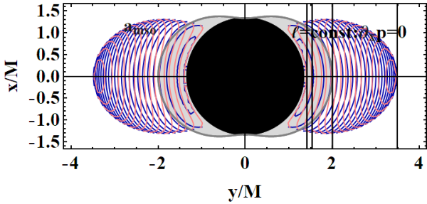

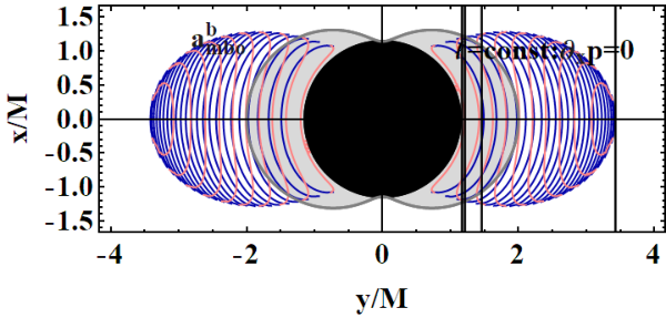
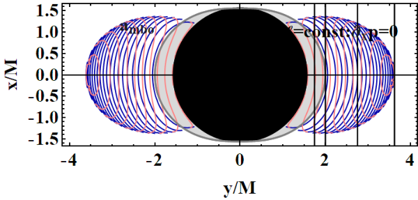
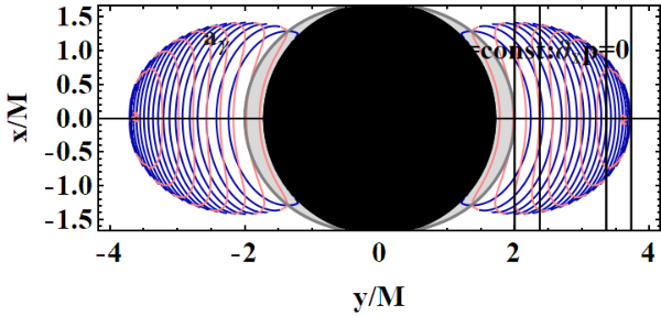

Figure 15: Study of the verticality of the disk, analysis of the vertical pressure gradients inside the disk. Black region is the BH, gray region is the outer ergosurface, and are Cartesian coodinates, different spins are represented –Figs (14). Curves are the solutions of where , providing a description of the vertical pressure gradient in the disks (there is (, on the equatorial plane there is ). The range of definition constant is bounded in a region dependent on the spin only. The boundary conditions are analyzed in Figs (32).
3.1.1 The tori verticality and disk exfoliation
Relevant aspects of the toroidal geometrically thick disks centered on the BH equatorial plane, are regulated by the dependence of the tori characteristics on the radial dimension, as the radial pressure gradients, which ultimately fixes the tori rotational law . For the tori orbiting in the ergoregion it is necessary to explore the vertical pressure gradients inside the disk. The disk verticality is in fact a significant factor for the accretion disks also in presence of the magnetic fields, and in many models of tori oscillation, as for the analysis of QPOs from accretion disks, which we face here in Sec. (3.2.1). The disk verticality in this model is regulated by the pressure -gradient and the curve of the extremes of pressure, including the points , the disks center , which is a maximum pressure point, and the minimum in the accretion flow at radius (for the overcritical, , configurations ) and the disk geometrical maximum– Figs (14). The curve relates the geometrical maxima and the extremes of the HD pressure, solution of (there is ). This curve depends on the BH dimensionless spin only.
The curves, solution of equation , are bounded in a range analyzed in Figs (32) where we show that the zeros and the maximal extensions of the range of definition for the solutions constant for the vertical gradient of the pressure are limited in a bounded region of the plane . More precisely, in Figs (15) we note how the vertical pressure gradient is limited by a surface dependent on the spin only. The extension of this range is largely unchanged by the BH spin as clarified in Figs (32).
The boundary curve is
| (15) |
represented in Figs (32), where the maximum is shown. It is evident that increasing the BH spin, the curves constant are confined in the ergoregion, the density of curves in the region increases approaching the horizon. For the limiting case of a static Schwarzschild BH, the boundary radius corresponds to (while the specific angular momentum and the energy function on this curve decreases with the spin, which can be seen analyzing the function and the function ).
To ensure the disk is entirely contained in , at a general plane we need to consider the condition . In fact, the necessary but not sufficiently condition to be satisfied for the outer part of the disk to be in the ergoregion (and also for the inclusion of the torus geometrical maximum) is , while this is a sufficient condition for the inner part of the disk to be included in the ergoregion. It is clear from Figs (15) that the curve of geometrical maxima and minima depends on ( on the equatorial plane) but also on the parameter (). There are two branches of the curve, one from and one . The torus approaches the BH poles rotational axes, when the torus geometrical maximum crosses the outer ergosurface.
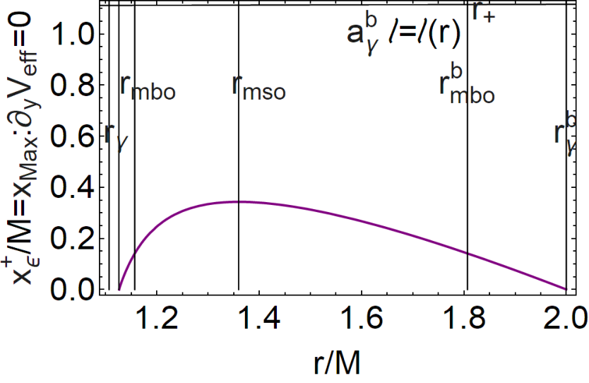

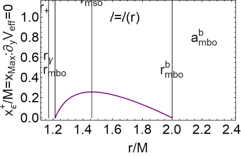

Figs (16) show the results of the analysis of the conditions for tori crossing the outer ergosurface considering the line of geometrical maxima. Radius is a limiting radius, being a maximum of the curve, as one value of the fluid specific angular momentum corresponds to two radii . Solutions (vertical axis) crossing of geometrical maximum line with the ergosuface as function of (outer horizon) are plotted (as solution of ). The analysis refers to critical (cusped) configurations. The smaller (larger) (the intersection of the toroidal surface with the static limit on ) is and the closest to the equatorial plane (rotational axis) of the BH is the crossing.

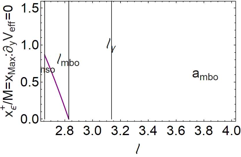


We argue that for the small surfaces crossing the outer ergosurface or in the ergoregion, the partially contained or dragged tori might undergo a form of instability, which could be also coupled with the usual internal processes, of the disk, induced by the geometry frame dragging, occurring in regions of the disks also far from the center of maximum pressure, leading to a process of disk ”exfoliation” (”peeling”). We consider this process more in details below. In Figs (16) we show the conditions to be satisfied for the geometrical maximum of the cusped surfaces intersecting the outer ergosurface. In Figs (17) we approach the analysis of the torus exfoliation studying the solutions of the problem of the disks crossing the outer ergosurface on , by its geometrical maximum (or the minimum) according to the analysis of Figs (15). We show the solutions (vertical axis), crossing of the line of geometrical maxima, defined by , with the ergosurface for fluid specific angular momentum , in the geometries of the set . The maximum heigh of the tori defined in the ergoregion is rather small. We note, in accordance with the analysis of Figs (16), (17), (18), that for the geometries with spins , and there is a solution of this problem for cusped tori which have specific angular momentum with . At larger momentum, , there is , and the torus can be also very large. The results of the analysis of the torus inner edge are in Figs (7). In the restricted range of tori parameters where cusped tori are, only geometries of a particular range of dimensionless BH spin admit tori with center of maximum pressure in the ergoregion, which is necessary but not sufficient condition for the intersection of the geometrical maxima with the ergosurface–see Figs (8).
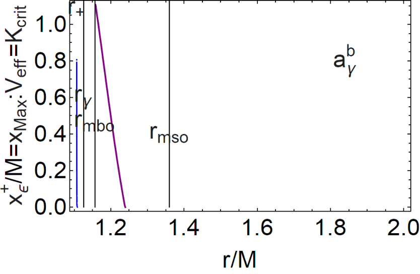

An analogue situation is in Figs (18) where is shown the crossing of the critical toroidal configurations (any point) with the outer ergosurface.


Notable radii and values of momenta are represented in Figs (19).


Figs (20) describe solutions of the problem , for two radii and for at different spins of the set . For , solutions are the radii , which are the center or the critical point of the tori as or , where . Therefore the analysis show the distance between maximum and minimum pressure points in the cusped disk, as well as the location of the points. The curves shown Figs (20) are bounded in the region delimited by and the radius where is the horizon curve in the plane . The solution of the problem for distinguishes the points such that for two tori with specific angular momenta respectively–see Pugliese&Stuchlík 2015.
3.1.2 Dragged disks thickness: influence of the dragging frame on the disk thickness
In Figs (15) and Figs (39) we show the results of the analysis of the disk verticality in terms of the polar gradient of the pressure, considering the lines of extremes of the HD pressure, which provide also the surfaces geometric maximum, obtaining clear indication of the maximum vertical extension of the torus in . The disk thickness is an essential parameter in the study tori oscillation processes, in the regulation of the instability processes and in the accretion. The analysis of Figs (21) clarifies the situation for the geometries of the set (represented Figs (14)).


Figs (21) show the geometrical thickness of the cusped tori in the ergoregion for the dragged surfaces and for tori close to the outer ergosurface for the BH geometries with spins in . In the definition of , is the geometrical maximum of the cusped toroidal surface, obtainable from the solution of and defined by the condition (the energy parameter at the cusp ), which is also studied in Figs (14), is the torus elongation on the equatorial plane–Figs (8), Figs (7). Because we restricted our analysis on the cusped tori, we assumed : for there is the limiting case of a proto-jet, for there is the limiting case of one ring torus located on the marginally stable orbit. It is evident how only tori for of the set have .
For larger , tori can be also very small, while for smaller tori, including partially contained tori in the ergoregion, are larger. For radii very close to the marginally bounded orbit, for any spacetime considered, there is a turning point in the tori thickness, i.e., at larger there is . As value is the limit for geometrically thick disks prevalently tori under this condition are small tori. However, for cusp close to , for all the spacetimes there is a region where (right range) and a second region (left range at closer to ) where .
3.1.3 Tori exfoliation
The Lense-Thirring effect of the Kerr geometry is expected to hugely affect partially contained and dragged tori (also if viscosity and radiation enter the play). The small tori can undergo a process induced by the dragging effects in the ergoregion, at different planes resulting in (almost vertical) fractiousness of the tori surface, which can combine with the accretion processes onto the central BH attractor, leading to a swarm of (initially corotating) particles and eventually photons, which can constitute a tori atmosphere. According to the initial data on the torus, they can escape in the outer region, remain trapped in the region , impacting back to the tori surface and environment (analogously to a Poynting–Robertson effect), and eventually be captured by the central BH (disk exfoliation). This process, relevant for the smaller disks, may also occur in combination with the Bardeen&Petterson effect in tori with a slight inclination with respect to the equatorial plane. In this regard it is necessary to reassess the ”pressure forces” in the disks orbiting in which, in the GRHD model with constant, are independent from the details of the polytropic equation of state, and depend only on the fluid effective potential gradients. The gradients of pressure represent the main factor for the formation and stability of the dragged tori (we also note there are no ZAMOs geodetics in the BH ergoregion). On the other hand, the pressure gradients are also the main factor to be evaluated for the exfoliation and the consequent formation of a possible atmosphere of (free) particles swarm. In this context it can be also important the role of external large scale magnetic field–see for example Kološ et al. 2021; Stuchlík&Kološ 2016; Kovář et al. 2016.
Here we do not focus on the particulars of the processes leading to the formation, reflection, or emission of particles and photons, but on the evaluation of the effectiveness of this process in the considered hydrodynamic models, giving thus a groundwork for the analysis of more complex systems. This process may also give rise to effective dissipative forces (or inducing internal turbulence), especially in small tori with a small inner elongation (distance between the maximum pressure point and the inner edges), and crossing the ergosurface at some plane , as considered for example in Figs (14), characteristic of the BHs geometries with spins . Clearly, these particles and photons interact with the BH environment, for example in the presence of a magnetosphere, with surrounding magnetic fields and other accreting materials. However, it is necessary to understand the characteristic time scales for the eventual destruction of the disk, which would depend on the mass (regulated by the parameter) and on the disk and BH specific momentum. In the context considered here, this phenomenon involves disks with , which can combine with jet and proto-jets emission, regulated by the limiting light surfaces provided by the solutions of – Figs (39). A particularly interesting situation would occur when as this condition, where the inner part of the disk is dragged and the outer part of the disk is fully contained or partially contained in the ergoregion, may imply the geometrical maximum of the disk approaches the outer ergosurface. Therefore in the process of torus exfoliation we can distinguish the following two cases:
- (I)
-
In the first case there is , where is the projection on the equatorial plane of the geometrical maximum of the torus. This condition is sufficient for partially contained tori with the inner region, , in . The first inequality, , is always satisfied, while condition occurs in the limit of .
- (II)
-
In the second case there is . We note that even with the geometrical maximum of the torus can be outside the ergoregion.
We also consider the following three cases for the toroidal configurations:
- (i)
-
correspondent to overcritical tori with an accretion throat (there is );
- (ii)
-
, correspondent to a cusped torus;
- (iii)
-
associated to a quiescent torus (there is )
where is the value of the parameter at the maximum of the fluid effective potential (minimum of the pressure). Tori in these three cases also have equal constant fluid specific angular momentum. Cusped tori are considered in the Figs (15)– first line-center panel. In some cases the toroidal configuration crosses the outer ergosurface on a point or for external (where is here the crossing that occurs on a point at ) along the toroid surface. These cases are characterized by two different scenarios concerning accreting matter colliding with the embedding tori materials. The small dimensions of the tori (see Figs (21)) allow to perform a first analysis in the hypothesis of free test particle from the tori surface. We shall assume free particles with initial conditions dictated by the toroidal configurations studied in Figs (15) from four regions of the configurations crossing the static limit, which are the set 1. the inner edge, 2. the accretion throat, 3. the outer edge, 4. the geometrical maximum). In this first analysis we do not consider the details of the different accretion mechanisms which may also involve plasmas particles and magnetic fields66 6 For the analysis of timelike orbits, integration can be done equivalently on two sets of equations. Considering derivation with respect to proper time , the constraint equation (normalization condition) can be included in the set of four equations and integrated numerically. The three equations for the particles coordinates can be numerically integrated solving the constraint for , according to the initial data. Note we numerically integrated the geodesic equations assuming zero pressure terms in Eq. (8) and the particles four-velocity with normalization condition . To fix the initial data of Table (1) from the toroidal models of Figs (23), particles inherit aspects of the torus configuration reflected in the particle motion initial data, that is we express (at the initial time) from the definition of Eq. (3) (expressed in terms of and ), with , where is from the torus model detailed in Figs (23). As we consider timelke particles, parameter coincides with the -parameter of the torus (this can also be tested by applying the constraint to the initial data, as done in the case of photon particles, used also for example for the cases where, for some particles models, there is ). We adapted the constraint to the case of photons, and parameters cannot be provided from the tori model as for timelike particles, depending on the particular reflection and emission model. We used and , in the initial data, expressed in terms of the parameters and, similarly to the timelike particles cases, with adapted to the torus, the normalization condition on the initial surface is used to recover the parameter .. Particles models considered here inherit the initial data from the tori construction (values of and parameters). Therefore particles leave the tori from different points of the toroidal surfaces (data set ). From the definition of and , we find expressed in terms of using definition , having settled according to the torus model and for the timelike particles coincident to parameter of the torus. Initial data is managed according to the equations set up solving the constrain at the initial time. (Note and are torus ”global” parameter in the sense that are constant on each toroidal surface). Particles are initially circularly orbiting on an orbit defined by the location and on the torus surface (there is no need to define explicitly ) according with , therefore and .
Therefore, according to the torus and the particle model, we fix , in , for simplicity we refer to these points as ”emission points”, with initial data , where is for any quantity evaluated at initial time . We consider the toroidal models of Figs (23). Using the Kerr geometry symmetries, there are two emission points obtainable in accordance with the reflection symmetries with respect to the BH rotation axis (coincident with the torus rotation axis) for the emission points on the equatorial plane, and four positions for emission points on planes different from the equatorial, found considering also the symmetry for reflection with respect to the disk equatorial plane (coincident with the BH equatorial plane, note there is no need to fix ). In the orbits representations of Figs (24) and (25) for convenience we used one or two emission points. Furthermore we considered the entire trajectory in the internal area of the disk to enlighten the trajectories impacting the disk, on its inner edge, as this back-reaction from the emission to the inner regions of the tori resolved eventually in photons and dust (or plasma) colliding with the toroid matter, being a characterizing factor of partially contained or dragged toroids. Particle leaving the surface can evolve in a swarm of particles created in an atmosphere wind around the torus surfaces. Or eventually, they can part from the torus, for example from the outer edge of the outer region crossing ergosurface as a wind of particles and photons, or part of the emission could impact on the torus surface if emitted from the inner region (note the model considered here is opaque, cooled with advection and with super Eddington luminosity).
In this analysis we should take into account the size of partially contained and dragged tori, studied in Figs (21), the torus maximum height and the location of the tori outer edge.
The torus maximum dimensions are constrained largely by the BH dimensionless spin. The reduced dimensions of the tori mean that the dragged surfaces are similar to globules where exfoliation should take start. Another important factor in this process is the back-reaction effect through tori self gravity for the huge tori, combined with accretion and runaway instability. The analysis of PPI or MRI for these tori should be also taken into consideration (Gammie 2004).
Runaway instability (RI), however, is an important process for thick disks orbiting SMBHs, particularly for partially contained and dragged surfaces. In this type of instability, the eventual rotational law constant, defining different tori model, can be significant. Neglecting the torus self-gravity, and using stationary models, RI can be studied with a fully relativistic hydrodynamics analysis. The RI features a sequence of varying mass BH phases following the mass transfer from the torus during the accretion and the consequent new status of the torus. The torus can become stable or unstable, depending on several factors as the mass ratio of the disk and the BH, if the BH is spinning, and most importantly the location of torus inner edge and cusp with respect to the central BH at the initial stage of the process. We expect therefore the RI be significant for dragged surfaces considered here and especially the partially contained tori, having the cusp close to the BH, but being large enough to interfere with RI with the eventual mass-transfer slowing-down and the torus exfoliation characterizing the smallest tori in . The RI is generally a very fast process enduring on a dynamical timescale of a few orbital periods. In this process the geometry changes consequently to the increase of the BH mass for accretion from the disk. It is then clear that there can be also a BH spin variation due to rotational energy extraction, via the Blandford–Znajek mechanism, where the amount of extractable energy depends on the disk mass and can be ejected in jets or winds observable for example in GRBs. (Some considerations on the extraction of rotational energy are in Sec. (3.3)). The accretion disk therefore adapts to the new situation leading possibly to a series of steady states. The torus inner edge plays a key role in this process, the disk filling its Roche lobe can transfer mass through the cusp. Following the geometry change, the cusp can stretch towards the horizon, slowing the mass transfer, which can eventually stabilize the toroid, or otherwise the cusp can move outwardly, into the toroid interior, increasing the mass transfer, eventually the toroid could be ”absorbed” by the central BH in a very fast process. The disk inner region, , regulates the two cases, therefore this analysis singles out the relevant tori .
In , we consider quiescent tori with , cusped tori and over critical tori with an accretion throat whose minima are given by the pressure extremes curve. Naturally we can evaluate the force term to which the particles of the different points of the toroidal surface are subjected by the pressure gradients in Euler’s law, in points other than the cusp where the free force hypothesis is guaranteed–Figs (22). It is expectable that the closer the inner edge is to the BH horizon, the more significant is the RI, which is therefore significant particularly for BH with high spins. In this case then, we note that tori with outer edge , represented in Figs (22), have inner edge closer to the and therefore far from the horizon (Abramowicz et al. 1983; Abramowicz et al. 1998; Korobkin et al. 2013; Font&Daigne 2002).
Analysis of Figs (24) and Figs (25), considers the BH geometry with spin , studying tori with specific angular momentum , considering the four toroidal configurations defined by four values of parameter of Figs (23). This first study of the particles can be implemented point by point on the surface. In Figs (23) the blue line sets the center and the geometrical maximum points of all the tori at and the minima of the accretion throats. Therefore, all the considered tori have at least the inner part of the disk contained in the ergoregion.


Figs (22) show the results of the analysis of the torus outer edge crossing the outer ergosurface on the equatorial plane, for cusped tori , with specific angular momentum and parameter . Tori having these characteristics can be observed only orbiting BHs with spin . Increasing the BH spin, the range of values of the parameters and , for quiescent or cusped tori , decreases according to the fact that the tori are corotating. Relation can be considered almost linear. The analysis shows a larger range of values for and , for BH with spin in a range centered on the value . The peculiarity of the geometries of this range is also shown in right panel, with the results for cusped tori. Note that cusped tori have equatorial elongation larger then the quiescent tori with equal specific angular momentum (a different case occurs for the overcritical tori having an accretion throat). The extended geodetic structure of this geometry is studied in Figs (2). Inner, outer edge and center of the tori of Figs (6) are shown as functions of the specific angular momentum. An alterative study of the outer edge, center and cusps of the tori is in Figs (7). The analysis is repeated in Figs (8) as function of the cusp radius . A prospect of the possible toroidal surfaces orbiting in these geometries is in Figs (15). Analysis of the disks verticality is in Figs (16), Figs (17) and Figs (19). Distance cusps-centers is considered in Figs (20), the von Zeipel surfaces are Figs (32).
Tori in Figs (22)-right panel have outer edge at . Curves show different characteristics of the cups and center of the tori in a region , defined by spins and , around the radius and shown in Figs (22). The tori cusp at variation of the BH spin remains relatively close to the limiting radius , increasing the distance in , being small tori. Tori are smaller and closer to the ergosurface for spins close to , and are relatively small for the larger spins where the cusp approaches the radius , maximum distance is reached in . The cusp decreases increasing the BH spin, approaching . Therefore increasing the BH spin the tori elongation increases.
However, the tori stability and tori exfoliation depend on their inner region, whose radial dimension is (the outer region is ). We observe that there is always , where is maximal in .
Tori studied in Figs (23) orbit around a BH with spin and they are defined by the following four models with fixed constant:
- -
-
(1): Torus , yellow curve in Figs (23), is defined by parameter (the torus is characterized by the presence of an accretion throat), and it is partially contained in (with the torus inner part).
- -
-
(2): Torus , blue surface in Figs (23), is a partially contained torus, characterized by an accretion throat defined by parameter. The torus geometrical maximum crosses the outer ergosurface.
- -
-
(3): Torus , green-dashed surface of Figs (23), is defined by , it is a partially contained torus characterized by a small accretion throat, crossing the outer ergosurface on a plane .
- -
-
(4): Torus , black surface of Figs (23), is the cusped torus with , which is a dragged surface, with the outer edge coincident with the outer ergosurface on the equatorial plane.
We set the initial data for the integration defining six particles models77 7 Note in the formulation of toroidal models of Figs (23) and initial data in Table (1) it is not necessary to integrate the equation for the torus surface. We have numerically integrated the condition of Eq. (9), fixing the two tori parameters , according to the tori topology and using the rotational law and the function to fix the parameters values. On the other hand, the inner and outer edges of the cusped tori, the torus center (maximum pressure point inside the disk), the geometrical maxima of the torus surface are in fact directly obtainable, these radii are given in Pugliese&Montani 2015 and for example in Pugliese&Stuchlík 2018a; Pugliese&Stuchlík 2019–see also (Abramowicz&Fragile 2013). listed in Table (1)
| 1. Torus , particles are initially located on the geometric maximum on a plane . |
|---|
| Data: |
| 2. Torus . Particles leave the crossing point of the torus with the ergosurface. |
| Data: |
| 3. From the torus . Particles leave the crossing point of the torus surface with the outer ergosurface. |
| Data: |
| 4. From the torus . Particles leave a point close to the cusp of the torus . |
| Data: . |
| 5. From the torus . Particles are initially located on the torus outer edge, coincident with the outer ergosurface. |
| Data: . |
| 6. From the torus , particles leave a point . |
| Data: |


In Figs (23) we consider particular toridal surfaces at different from the set of Figs (14)–(upper line central panel). The analysis is a first simple attempt to consider the swarm of free particles and photons which is grounded on the reduced dimension of the tori in the ergoregion and the model of zero-pressure fluid at the tori edges–see Figs 21). We have used same approximation in Sec. (3.2.1) for the analysis of the oscillatory models of the torus using the characteristic Keplerian frequencies to discuss the adaptability of QPOs models on these structures.


In general the test particles hypothesis is of astrophysical significance, also in the case of a tori atmosphere. In this situation we can also combine in characteristics processes of these tori as the Poynting--Robertson effects for partially included and dragged surfaces88 8 The radiation field carrying out energy and momentum interacts back with the accretion disk plasma. The radiation field induces a radiation pressure which combines with a radiation drag force (which is the Poynting-Robertson effect), and the mass transfer during accretion. We should also note that the tori considered here are opaque and super-Eddington. The radiation drag can act as dissipative force for the orbiting matter, removing energy and angular momentum. The Poynting-Robertson effect can remove angular momentum and energy from small-sized test particles. Test particle radial motion is therefore affected by the Poynting-Robertson effect and radiation pressure and the accreting matter can lose angular momentum combining to accretion. (It should be noted that Poynting flux (in presence of magnetic field) carries away from the BH energy and angular momentum, combining in the BH evolution with the accretion.) There can be therefore (radiatevely and thermally) outflows and inflow followed eventually also by a change into the disk structure, considering outgoing or ingoing radial photon flux. (Igumenshchev 2008; Bini et al. 2011; Bini et al. 2015; Lee 2001; Ballantyne&Everett 2005; Zanni et al. 2007c; Pudritz et al. 2007; De Falco et al. 2020) .
We show some results considering light-like particles from the torus surface and with fixed initial parameters, using the constraint and the definition of . We used Eq. (4) for the photon to obtain initial data , determined by conditions on tori parameter and assuming the circular motion symmetries preserved, where there is and , determined by parameter and , the first fixed by the torus, while the second is fixed for the timelike particle by the -parameter of the torus. Eq. (4) does not differ for photon and timelike particles, defined by and with the definition of Killing fields. We considered , using for timelike particles parameters and . For the photons , the initial data has been fixed using the normalization condition used also in the set of equation to be integrated. We also considered the metric symmetries for the two solutions in .


Details of particles model 1., 2. and 3. of Table (1) are shown in Figs (25). Models 4., 5. and 6. considering particles on the torus and BH equatorial plane are shown Figs (24).
As exemplified by the cases studied in this example, particles follow three classes of trajectories: particles can leave the ergoregion; particles can remain trapped in the inner region (leading to collision with torus inner edge), or be absorbed by the BH. Photon motion is shown in Figs (26), (27). Particle models of Table (1) have been considered for the initial locations and the tori models. The disk exfoliation is based on the free particles hypotheses, grounded on low pressure gradients, Lense-Thirring effect and small tori sizes, (a further open question concerns the process time scale for the total destruction of the dragged torus). The example of Figs (26), (27) has therefore to be understood as indicative, and the analysis should be framed considering the emission-reflection processes from the disk surface.


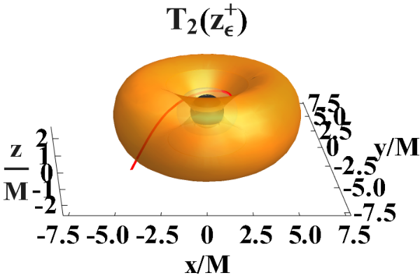

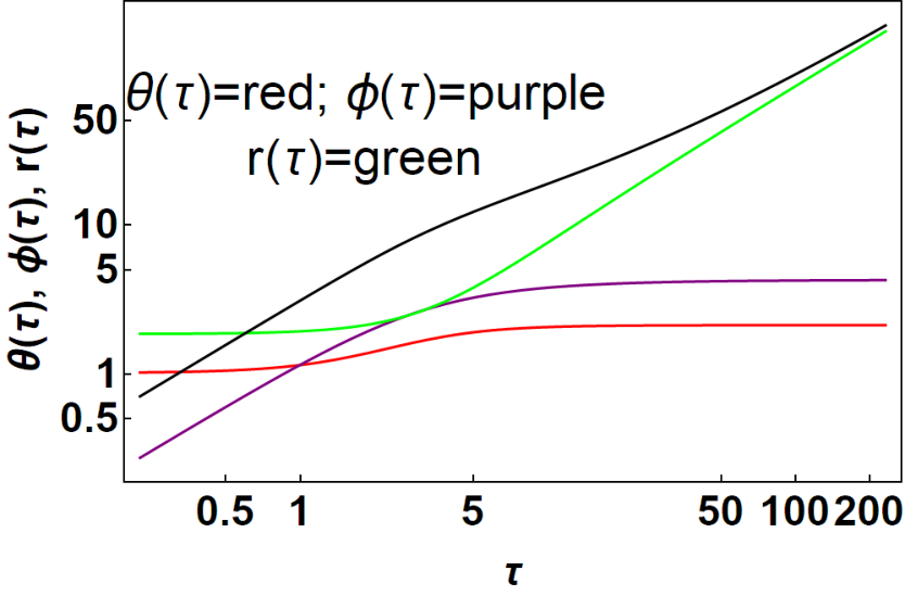


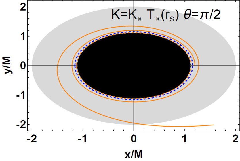

3.1.4 Extreme configurations: multi-tori, proto-jets and tori
On the sidelines of this analysis we also consider the proto-jets existence in . An issue that can affect stability of tori orbiting in is the possibility that several orbiting toroidal configurations may be formed in aggregates of toroids orbiting the central BH, occurring, for example, in composed systems of tori agglomerates as in the eRAD framework (Pugliese&Stuchlík 2015; Pugliese&Stuchlík 2017), developed as aggregates of axisymmetric, corotating and counter-rotating toroidal configurations, coplanar and centered on the equatorial plane of the central Kerr attractor in AGNs-Figs (28).

Figs (28) show for the BH spacetime with , the case of three closed configurations, the inner cusped torus contained in the ergoregion as in Figs (14). The outer critical torus is counterrotating, the middle of the triplet is quiescent and corotating. This is a case of double accretion onto the central BH with a middle screening torus.
It is clear that each toroidal component of the aggregate of partially contained or dragged surfaces is constrained according to the analysis of Secs (3.1). Especially tori orbiting around faster rotating BH can rise to collision. These tori would be extremely small and at close distance (i.e. small displacement where is the inner edge of the outer torus while is the outer edge of the inner torus). There is , and this property suggests that the dragged tori distribution (density of tori centers in a region around the central BH) has no extreme as function of for any spin , if the agglomerate does not vary with the spin or radius. However, this may not be the case for partially contained configurations because of the presence of the radius in the stability range for the centers of tori. Curve represents an ”accumulation” point for the tori centers. Radius would be a center for the configuration with specific angular momentum in the range , where proto-jets are possible. Correspondingly, there is the radius for the proto-jets cusps in the geometries , where , and ; in this spin range there is , and for larger spin. Radius is a center for tori in correspondent to unstable points – see Figs (29) and Figs (19)- Figs (2). On the other hand, there is a BH geometry with where , in the range .


Then and the quiescent torus inner edge is , which can be in ergoregion also for relatively small BH spin, opening an interesting possibility for jet emission and the role of the ergoregion, which would be suppressed at large spin. The possibility of existence of configurations with the solutions of , points of accumulation of pressure , in the ergoregion, and therefore of inner edge of , has been investigated in Figs (30). It is clear that this possibility is regulated by the spins and . In the critical points lie in the ergoregion.


3.2 Characteristic frequencies


The investigation of the disk verticality in the ergoregion includes the exploration of the characteristic frequencies affecting the torus. The analysis in Figs (31) shows the vertical frequency in the ergoregion considering therefore the frame dragging for very high spinning BH, as clear by the presence of extreme of as function of the spin and as function of . Concerning more generally the tori dynamical oscillations it should be said that the spectrum modes are not completely studied. The axisymmetric, incompressible modes related to global oscillations comprise the epicyclic frequencies. The Keplerian, radial and vertical angular frequencies take the form (Stuchlík et al. 2013)
| (16) |
The frequencies are treated in various so called geodesic epicyclic models of HF QPOs (Straub&Sramkova 2009; Stuchlík et al. 2011; Stuchlík et al. 2013; Stuchlìk et al. 2017; Šramková et al. 2015; Stuchlík et al. 2005; Stuchlík et al. 2007a; Stuchlík & Kološ 2016; Stuchlík et al. 2011; Stuchlík et al. 2007b; Török et al. 2016a; Török et al. 2016b; Török et al. 2011; Kotrlová et al. 2008; Kotrlová et al. 2017; Török& Stuchlík 2005). We apply then and the results are presented in Figs (31)–(36), frequencies are given with respect to the Boyer-Lindquist time coordinate , i.e. with respect to an observer at infinity. (Note the frequencies in the proper time can be obtained by multiplying for .). Frequencies on the static limit are shown in Figs (35) as function of the central BH dimensionless spin . The frequency is the relativistic orbital angular frequency. The last two frequencies derive from the first derivative in the radius and angle respectively, of the effective potential of the geodesic motion. Their properties were extensively studied in Török& Stuchlík 2005
In this model the entropy is constant along the flow. According to the von Zeipel condition, the surfaces of constant angular velocity and of constant specific angular momentum coincide and the rotation law is independent of the equation of state. This property of the rotational law is linked to scale-times of the main physical processes involved in the disks, the accretion mechanism for transporting angular momentum in the disk, and the turbulence emergence dependent the magnetic fields and on the vertical structure of the torus (Abramowicz 1971; Chakrabarti 1990; Chakrabarti 1991; Zanotti&Pugliese 2015; Lei et al. 2008). The von Zeipel condition is also to be considered for the determination of the analytical models for the magnetic field in the magnetized plasma fluids(Zanotti&Pugliese 2015). Von Zeipel surfaces are shown in Figs (32).


Essentially the application of the so called Boyer condition within the conditions of the von Zeipel results reduces to an integrability condition on the Euler equations. In the case of a barotropic fluid, the differential equation (8) can be integrated reducing to a gradient of a scalar, which is possible if and only if . (Dragged tori are far from the quasi-spherical conditions). In general in these models of accretion disks the angular momentum of matter in the disks is considered to be sufficiently high for the centrifugal force to be a predominant component of the four forces regulating the disks balance (centrifugal, gravitational, pressure and magnetic forces, and eventually dissipative effects). This holds for situations where the gravitational background is generated by a SMBHs shaping morphology and a great part of dynamics on (micro and macro-scopical scale of) the disks. In general accretion disks, there must be an extended region where there is in the same orbital region (explicitly including counterrotating fluids on Kerr background). This limiting condition is assumed to hold for a general accretion torus with a general angular momentum distribution. The Bondi quasi-spherical accretion constitutes a situation when the condition is not fulfilled. In the Bondi quasi spherical accretion, the fluid angular momentum is everywhere smaller than the Keplerian one and therefore dynamically unimportant. However, the models under examinations here are based on a full GR onset for each RAD toroid, where in fact there exists an extended region where the fluids angular momentum in the torus is larger or equal in magnitude than the Keplerian (test particle) angular momentum. Frequencies of Eq. (16) are then combined the lower and higher frequency peaks in the particles models of the QPOs emission.
3.2.1 On the origin of the QPOs emission and the ergoregion
We discuss the possibility presented in different literature that the origin of the QPOs (Quasi-periodic oscillations) emission could be attributable to and immediately traceable to the oscillatory phenomena reducible to the test particles, considering the case of particles in the ergoregion(Stuchlík et al. 2013). This hypotheses is plausible in these models of dragged and partially contained tori as they can be considered small tori, relatively close to the maximum pressure radius constituting the torus center. The small geometric thickness of the disks is investigated in Figs (21), although the thickness parameter considered for the construction on QPOs emission model based on the tori geometrical thickness has been discussed in Török et al. 2016a; Straub&Sramkova 2009.
QPOs are observed in the X-ray brightness at low (Hz) and high (kHz) frequencies. Observed QPO frequencies are associated in many models with frequencies of orbital and oscillatory motion of the particles from accretion disk matter. The peaks of high frequencies turn to be near the orbital frequency of the marginally stable orbit extreme, limit for the inner edge of thin disks. The upper and lower frequencies of the peak are in the particles geodesic models expressed in terms of the radial and vertical oscillations and the azimuthal frequency. Particular attention is given to recognize the emergence of the twin HF QPOs with resonant frequency ratios . The observed ratio of the twin peak frequencies and other resonances characterized by ratios as . could explain observed QPOs frequencies (with same ratio), considering the combinational frequencies, occurring in the inner parts of accretion flow around a black hole Stuchlík et al. 2013. Therefore we shall consider the resonant frequency ratios , , , , .
The cusped tori are associated with the cusp point of the minimum null-pressure. In this respect the torus cusp could be possibly connected to QPOs emission.


The individual QPO models frequencies considered here are functions of three fundamental frequencies of perturbed circular geodesic motion and are:
| (17) | |||
| (18) | |||
(RE) and (Kepl) models are investigated in Figs (36). Frequencies on the static limit are in Figs (35). The radial frequency is well defined, , for , where it vanishes, determining orbits stability for radial oscillations around the point of the perturbed particle. We consider this problem and various oscillation models as in Eqs (17) in the ergoregion, where for , including geometry and .


In Figs (34) we show the models in the BH geometry in comparison with different resonant ratios, in Figs (33) we show the models in the BH geometry . Each frequency model we study is borrowed from a specific context from which they are derived including slender tori and hot spot models (assuming radiating spots in thin accretion disks). Therefore frequencies used in the fit of the models are therefore expressions of particle frequencies that can demonstrate Keplerian and epicyclic frequencies: (WD) is for ”warped disk” model introduced for oscillatory modes in a warped accretion disk. is for tidal disruption model (related to tidal disruption of accreting inhomogeneities) (Kostic et al. 2009). TP and TP1 are for total precession models. , an are for relativistic-precession models, attributing the HF QPOs to modes of blobs in the inner parts of the accretion disk. (RE) is for ”epicyclic resonance” model dealing with radial and vertical epicyclic oscillations, and the (Kepl) for ”Keplerian resonance” model assuming a resonance between the orbital Keplerian motion and the radial epicyclic oscillations (Stuchlìk et al. 2017; Stuchlík & Kološ 2016; Stuchlík et al. 2007b; Török& Stuchlík 2005; Kotrlová et al. 2017; Török et al. 2016b; Šramková et al. 2015; Stuchlík et al. 2013; Török et al. 2011; Stuchlík et al. 2011; Kotrlová et al. 2008; Stuchlík et al. 2007a)


3.3 Tori from polytropic fluids and the ergoregion
In this section we specify the polytropic equation of state (EoS) for dragged tori. An interesting issue to be investigated is whether the frame dragging of the Kerr spacetime may differentiate dragged and partially contained tori or configurations close to the outer ergosurface with different equations of state, for example if the polytropics can affect differently dragged tori. We consider a polytropic equation of state, assuming the pressure be a function of the matter density : , where and is the polytropic index. In Pugliese&Montani 2015 different polytropic EoS for tori were studied, distinguishing classes in relation with the tori parameters ranges and the locations, here we re-focus on this concept in relations with tori in the ergoregion. It has been shown that there is a specific classification of eligible geometric polytropes and a specific class of polytropes is characterized by a discrete range of values for the index , (Pugliese&Montani 2018; Frank et al. 2002; Pugliese&Montani 2015; Stuchlík et al. 2009; Stuchlík et al. 2020). For the matter density there is
| (19) |
where , which is independent from . We consider here . The following two cases occur:
- 1.
-
There is , which is for , where for and for .
- 2.
-
There is , which is for , within the condition for , and the condition for . The polytropic index satisfies the condition where and , and .
(Note, the case 1. includes polytropes with index .).
3.3.1 Polytropic fluids and tori energetics
We consider tori with polytropic fluids: , providing an estimation of the mass-flux, enthalpy-flux (evaluating also the temperature parameter), and the flux thickness based on geometric consideration only on the thick disks in the ergoregion or close to ergoregion–see Abramowicz&Fragile 2013; Abramowicz 1985. In details, these quantities are listed in Table (2).
| Quantities | |
| [-quantities]: | [-quantities]: |
Parameters within the constraints constant, fix a polytropic-family. Then , with being the polytropic index. We use the fact that the pressure forces are vanishing at the edges of the accretion torus. These quantities can be express in the general form . The depends on the location of the inner edge of the accreting torus, being determined only by the angular momentum, and on the radius which is related to the thickness of the matter flow: corresponds to the accreting point , while is directly associated to the accreting flux thickness, where . In , and are different functions of the polytropic index and of the polytropic constant . The mass flow rate through the cusp (mass loss, accretion rates) , and the cusp luminosity (and the accretion efficiency ), measuring the rate of the thermal-energy carried at the cusp could be expressed as quantities, or alternatevley -quantities, as in Table (2). - and -quantities of Table (2) are evaluated for corotating tori in Figs (37) providing a simple way to evaluate the trends of these functions of the BH spin and the cusp location.


The quantities at are evaluated according to , where in Figs (37). The behaviour of the curves at different spins as functions of (therefore as functions of the specific fluid momentum) is qualitatively independent from variation of (an increase of correspondent to a lowering of parameter over the critical maximum value and lowering of the matter level towards the cusp is associated to similar qualitative behaviour of the curves and decrease in magnitude). We note that clearly the choice of corresponds to the choice of a point on the curves at as in Figs (14). An analysis of the and location of the critical points for different BH spins in relation to the possibility of multi-orbiting tori around the central BH, consisting by both corotating or counterotating fluids, can be found in Figs (5). We can note that there is an increase of the spin corresponding to a decreases of the range ; on the contrary, the curves increase due to increasing the distance from the BH of the disk cusp which corresponds to the increase of the specific angular momentum (at fixed BH spin ). Despite the reduced dimensions of the dragged configurations it is clear that and are quite large inside the ergoregion . Considering Figs (2) we can see that the analysis of cusped configurations in Figs (37) is in agreement with the existence of the cusp in the ergoregion at , and . This analysis, however, does not take into account both the deviations present from the perfectly stationary situation, and the fate of the flow in free falling after the cusp. We can analyze this case, taking into account that that region corresponds in fact to the situation of minimum hydrostatic pressure.


The extractable rotational energy .
In Figs (38) the analysis has been developed showing explicitly the relations between the dragged toroidal surfaces characteristics in the ergoregion and the maximum extractable rotational energy from the BH horizon, through the analysis of the leading function and the energy function . The plots show the situation one might expect in a phase prior the total extraction of the energy from the BH. We start by considering the spin function (Pugliese&Stuchlík 2021):
| (20) |
relating the dimensionless BH spin to the dimensionless ratio , (total released rotational energy versus BH mass measured by an observer at infinity). We are assuming a process ending with the total extraction of the rotational energy of the central Kerr BH. Considering and the mass and angular momentum of the initial state of the BH, the upper limit for of the energy extraction from a stationary process bringing the BH at the state is . The BH angular momentum in the new state is zero. All the quantities therefore are evaluated at the state prior the process, which implies that all the quantities evaluated here inform on the status of the BH-accretion disk system at its stationary state . We use the approach introduced in Daly 2009; Pugliese&Stuchlík 2021, which is , based on the definition of BH irreducible mass and rotational energy, and it is independent from the energy extraction mechanism, using the BH classical thermodynamical law.
Considering the dimensionless rotational energy as ( is the irreducible mass), with quantities evaluated at the stationary state prior the process, we obtain the restricted range , where limiting therefore the energy extracted to a superior of of the mass , where at the state (prior the extraction) there is an extreme Kerr BH spacetime. The larger extractable rotational energy is related to the BH with the smallest dragged tori, including the dragged or partially included tori in the ergoregion. Plots show also details on the location of the inner edge and center of maximum pressure, in the possible configurations around the BH. The small dimension of tori is intended in the following sense: it is clear from Figs (21) that the thickness of tori is larger for larger BHs spin for the parameter , the limit being associates to cusps very close to the , therefore to very large . For , we find tori with greater thickness in geometries of smaller BH dimensionless spins. From Figs (22) and from the analysis of conditions for the outer edge of the cusped tori to be coincident with the static limit , it is clear that there is a total disk elongation larger for the larger BH spins, while the inner elongation decreases with the spin (with respect to the observers at infinity) 99 9 In relations to BHs of the set , there is , , , , , , where is the maximum extractable rotational energy, occurring for an extreme Kerr BH..


Figs (39) show the solution of the zeros of radial gradients of pressure, which is related to the definition of . The analysis considers the surfaces constant, where the effective potential is function of Cartesian coordinates and we can note the role of the marginally stable orbits–see also Figs (32). In Sec. (A) we include some notes on the stationary magnetized tori in the ergoregion, considering the GRHD tori with a toroidal magnetic field according to the Komissarov solution (Komissarov 2006).
4 Conclusions
In this work we investigated orbiting extended matter configurations in the ergoregion of a spinning black hole, introducing in Sec. (3.1) the concept of dragged tori and partially contended tori. To this end, we considered corotating perfect fluids tori, constituting geometrically thick accretion disks, using the disk model detailed in Sec. (2) for tori orbiting a central Kerr BH.
It is argued that the smaller dragged tori could be subjected to a characteristic instability, disk exfoliation, consequence of the geometry frame-dragging. We discussed this hypothesis assessing the tori features for the occurrence of this phenomena, the possible outcomes as particle and photon emission, or in an enhanced accretion. This process is expected to lead to the destruction of the torus in combination with accretion, emission and other processes typical of the regions very close to the black hole horizon as, for example, the Runway Instability. An important parameter for the tori exfoliation is the torus verticality, given by the evaluation of the dragged torus geometrical thickness. In Sec. (3.1.1) we face this aspect, discussing also tori possible formation, and providing in Sec. (3.1.2) an throughout investigation of the dragged disks thickness and exploring the influence of the dragging frame on the disk thickness. Results of the analysis of the outer edge location with the respect to the static limit are in Figs (6,7,8,22). The results of the investigation of the inner edge location with the respect to the static limit are in Figs (10) and (9).
The analysis eventually provides indications on the attractors where dragged tori can be observed, and tori characteristics, according to the central attractor dimensionless spin. We individuated five classes of geometries, as in Figs (2), defined according to the BHs spin–mass ratios, bounded by the spins , and regulating the constraints on the location of the extremes of the pressure in the tori–Figs (14),(4) and (19). We studied the toroids in each of these classes. Configurations orbiting in the geometries defined in are shown in Figs (14) The conditions for the tori outer edge to be in , in the different geometries of the set , are shown in Figs (6), for cusped tori are in Figs (7), and in Figs (8) where the conditions are expressed in functions of the disks inner edge, , location. We provided in Figs (7,8,9,10) indications on the torus inner region elongation, , the most active and significant part of the tori for this analysis (large tori inner elongation are expected for small BH spin). While results on the torus outer edge coincidence with the static limit are in Figs (7,8,22).
On the other hand, the pressure gradients are also the main factor to be evaluated for the exfoliation and the consequent formation of a possible atmosphere of free-particle swarm. In order to asses the reliability of an eventual process of disk exfoliation we studied in Sec. (3.1.1) the pressure gradients in the disks, results are in Figs (13), (14),(15),(32),(16),(17),(18),(7). In Figs (15) and(39) we show the results of the analysis of the disk verticality in terms of the polar gradients of the pressure, considering the lines of extremes of the HD pressure, providing also the surfaces of geometric maximum, obtaining therefore a clear indication of the maximum vertical extension of the torus in the ergoreigon. Figs (21) summarize the results on the dragged tori geometrical thickness, distinguishing faster spinning and slower spinning black holes, and the situations where the inner Roche lobe of the tori is thicker then the outer Roche lobe for the dragged cusped tori. In Sec. (3.1.3) we explored the process of tori exfoliation considering five tori models, six particle models from four regions of the configurations crossing the static limit. We considered quiescent (inert) tori (topologically regularly surfaces) and cusped tori, characterized by the HD instability driven by a Paczyński mechanism. The accretion occurs through the torus cusp (from the outer Roche lobe of the disk ). On the sidelines of this analysis we also considered in Sec. (3.1.4) the proto-jets existence in , and extreme configurations as agglomerates of toroids orbiting the ergoregion constituting aggregates of corotating tori which can collide .
Dragged and partially contained tori have been also studied in relation to the QPOs emissions from the tori inner edges. More precisely, the characteristic frequencies of the toroids are studied in Sec. (3.2) and in Sec. (3.2.1) we discuss the origin of the QPOs emission from toroids in the ergoregion. We focused on the resonant frequency ratios , , , , and frequencies used to the fit of the models are expressions of particle geodesic frequencies of Eqs (17) related to dragged or partially contained tori (with torus inner region contained in the ergoregion). Some results are in Figs (34)– (36).
In Sec. (3.3) we specified the polytropic equation of state for dragged and partially contained tori, investigating how the frame dragging of the Kerr spacetime could differentiate dragged and partially contained tori with different values of the polytropic index. Discussion on some aspects of tori energetics for these tori is in Sec. (3.3.1). We provided an estimation of the flux thickness, mass-flux and enthalpy-flux basing on geometric considerations for dragged and partially contained thick disks. These toroids can be observed orbiting black holes with dimensionless spin .
In Sec. (3.3.1), we also discussed the relations between the dragged tori in the ergoregion and the maximum extractable rotational energy from the BH horizon, showing the situation of the state prior the total extraction of the energy from the BH, considering the approach introduced in Daly 2009 focused on the definition of SMBH (irreducible) mass function and the definition of rotational energy. Finally, in Appendix (A), we included in the GRHD model developed in Sec. (2) a toroidal magnetic field a la’ Komissarov (Komissarov 2006), developing the analysis on the stationary magnetized tori in the ergoregion. As mentioned in Sec. (3.1.3), disk exfoliation could combine with others tori characteristics processes as the Poynting–Robertson effects for partially included and dragged surfaces. Runaway instability is another major process for dragged thick disks orbiting SMBHs. We intend to deepen the relation with the Bardeen–Petterson effect, for tori having a slight inclination with respect to the equatorial plane, in regards to the possible origin on an inner corotating dragged or partially contained tori.
Data Availability
No new data were generated or analysed in support of this research.
Appendix A Notes on stationary magnetized tori in the ergoregion: the toroidal magnetic field
The study of the magnetized surfaces with toroidal magnetic field is an interesting issue of the toroidal configurations we consider here. The presence of a magnetic field with a relevant toroidal component can be related to the disk differential rotation, viewed as a generating mechanism of the magnetic field (Komissarov 2006; Montero et al. 2007), The Komissarov solution is a well known and widely used magnetic field solution based on the construction of a toroidal magnetic field considering the set of results known as von Zeipel theorem- (Komissarov 2006). Here we consider the possibility that such field could be defined in the ergoregion. We re-consider briefly the onset developed in Pugliese&Montani 2013; Pugliese&Montani 2018. We also refer to Pugliese&Montani 2013; Hamersky&Karas 2013; Karas et al. 2014; Pugliese&Montani 2018; Adamek&Stuchlík 2013 where this solution is dealt in detail in the context of accretion disks. We consider an infinitely conductive plasma, with where is the Faraday tensor and , where is the fluid four-velocity and is the magnetic field with and .
The Euler equation for this system can be exactly integrated for the background spacetime of Schwarzschild and Kerr BHs with a magnetic field and magnetic pressure
| (21) | |||
| (22) |
where is the fluid enthalpy, and are constant-Komissarov 2006; Montero et al. 2007. (A barotropic equation of state is assumed). Eq. (9) has been used in second term of equation 21. According to our set-up we introduce a deformed (magnetized) Paczyński potential function and the Euler equation (9) becomes:
| (23) | |||
| (24) |
We therefore consider the equation for the function and we introduce the function
| (25) |
The toroidal surfaces are obtained from the equipotential surfaces, for the potential which, for , reduces to the effective potential for the non-magnetized case in Eq. (9). The tori are regulated by the modified rotational law , for counterrotating and corotating magnetized fluids respectively- where there is . We rephrase the problem introducing an adapted function , whose values constant, provide the parameter defining the torus. Re-considering the equation for the hydrostatic pressure critical points, solution represents the values of as a function of , for which critical points of the function exist:
| (26) |
(with and and ), giving the tori centers and, eventually the tori cusps. (A negative solution for may appear for .).


We are interested to the conditions for the magnetic field, defined in Eq. (21), is well defined in the ergoregion at any plane constant. It is simple to see that the magnetic pressure, within the condition assumed on the enthalpy, is always positive. We note that, although the magnetic field is independent from the effective potential function , it depends implicitly on the parameter. In Figs (40) we considered the field in relation to tori present in the ergoregion. The definition of the magnetic field is delineated by the light-surfaces, solutions of , which provide solutions in the ergoregion–Figs (39). (The photon circular orbit on the equatorial plane , is a particular relevant surface.). The field is not well defined approaching the horizon . There is where , and the problem is reduced to find the solutions of the equations for the frequencies of the stationary observers. Light surfaces have frequencies . Spacelike solutions are given for and (on all the planes ). On the ergosurface the condition is as .
References
- Abramowicz (1971) Abramowicz M. A. 1971, Acta. Astron., 21, 81
- Abramowicz (1985) Abramowicz, M. A. 1985, Astronomical Society of Japan, 37, 4, 727-734
- Abramowicz et al. (1983) Abramowicz, M. A., Calvani, M. & Nobili, L. 1983, Nature, 302, 597–599
- Abramowicz&Fragile (2013) Abramowicz M. A. &Fragile P. C. 2013, Living Rev. Rel.,16, 1
- Abramowicz et al. (1998) Abramowicz M. A., Karas V., Lanza A. 1998, A&A, 331, 1143
- Abramowicz et al. (1996) Abramowicz M.A., Lanza A., Percival M.J. 1996, Astrophys. J., 479, 179
- Adamek&Stuchlík (2013) Adamek K.& Stuchlík Z. 2013, Class. Quantum Grav. 30, 205007
- Allen et al. (2006) Allen, S. W., Dunn, R.J.H., Fabian, A.C., et al. 2006, MNRAS, 1, 372, 21
- Ballantyne&Everett (2005) Ballantyne D. R. & Everett J. E. 2005, Astrophys. J. 626, 364-372
- Bardeen&Petterson (1975) Bardeen J. M. & Petterson J.A. 1975, Astrophys. J., 195, L65.
- Bekenstein (1975) Bekenstein J.D. 1975, Phys. Rev. D, 12, 3077
- Bini et al. (2011) Bini D., Geralico A., Jantzen R. T., Semerák O. and Stella L. 2011, Class. Quant. Grav. 28, 035008
- Bini et al. (2015) Bini D., Geralico A., Jantzen R. T., Semerák O. 2015 , MNRAS, 446, 2317-2329
- Blaes (1987) Blaes O. M. 1987, MNRAS, 227, 975-992
- Blandford&Znajek (1977) Blandford R. D., Znajek R. L. 1977, MNRAS, 179, 433
- Boyer (1965) Boyer R. H. 1956, Proc. Cambridge Phil. Soc., 61, 527
- Bugli et al. (2018) Bugli, M., Guilet, J., Müller, E., et al. 2018, MNRAS, 475, 108
- Chakrabarti (1990) Chakrabarti, S. K. 1990, MNRAS , 245, 747
- Chakrabarti (1991) Chakrabarti S. K., 1991, MNRAS, 250, 7
- Charbulák&Stuchlík (2018) Charbulák D., Stuchlík Z., 2018, EPJC, 78, 879.
- Daly (2009) Daly R. A. 2009, Astrophys. J., 691–L72-L76
- De Falco et al. (2020) De Falco V., Bakala P. , and Falanga M. 2020, Phys. Rev. D 101, 124031
- Fishbone&Moncrief (1976) Fishbone, L. G., Moncrief, V. 1976 Astrophys. J., 207, 962
- Font&Daigne (2002) Font, J. A. & Daigne, F. 2002, MNRAS, 334, 383
- Frank et al. (2002) Frank J., King A., Raine D. 2002, Accretion Power in Astrophysics, (Cambridge University Press, Cambridge 2002)
- Frolov&Zelnikov (2011) Frolov V. P., Zelnikov A. 2011, Introduction to Black Hole Physics, (Oxford University Press, 488, 2011)
- Gammie (2004) Gammie C. F. 2004, Astrophys. J., 614:309–313
- Gariel et al. (2013) Gariel J., Marcilhacy G. and Santos N. O. 2013, Astrophys. J. 774, 109
- Hamersky&Karas (2013) Hamersky J.&Karas V. 2013, A&A, 555, A32
- Hawking (1971) Hawking S.W. 1971, MNRAS, 152, 75-78
- Hawking (1976) Hawking S.W. 1976, Comm. Math. Phys. 43, 199 (1975) Erratum - ibidem 46, 206 (1976)
- Hawking&Ellis (1973) Hawking S. W. & Ellis G. F. R. 1973, The large scale structure of space-time, (Cambridge University Press, Cambridge, 1973)
- Igumenshchev (2008) Igumenshchev I. V. 2008, Astrophys. J., 677, 317
- Karas et al. (2014) Karas V., Kopacek O., Kunneriath D. & Hamersky J. 2014, Acta Polytech., 54, 6, 398
- Kawakatu&Ohsuga (2011) Kawakatu, N., Ohsuga, K. 2011, MNRAS, 417, 4, 2562-2570
- King et al. (2005) King A. R., Lubow S. H., Ogilvie G. I., Pringle J. E. 2005, MNRAS, 363, 49–56
- King&Nixon (2018) King A. and Nixon C. 2018, Astrophys. J., 857, 1, L7
- Kološ et al. (2021) Kološ M., Tursunov A., Stuchlík Z. 2021, PhRvD, 103,
- Komissarov (2006) Komissarov S. S. 2006, MNRAS, 368, 993
- Komissarov (2009) Komissarov S. S. 2009, J. Korean Phys. Soc., 54, 2503
- Korobkin et al. (2013) Korobkin, O., Abdikamalov, E., Stergioulas, N., et al. 2013, MNRAS, 431, 1, 354
- Kostic et al. (2009) Kostic, U., Cadez, A., Calvani, M., Gomboc, A. 2009, Astron. Astrophysic, 496, 30
- Kotrlová et al. (2008) Kotrlová A., Stuchlík Z.&Török G. 2008, Class. Quantum Grav., 25, 225016
- Kotrlová et al. (2017) Kotrlová A. , Šrámková E., Török G. 2017, et al, A&A, 607, A69
- Kovář et al. (2016) Kovář J., Slaný P., Cremaschini C., Stuchlík Z., Karas V., Trova A., 2016, PhRvD, 93, 124055
- Kozłowski et al. (1978) Kozłowski M., Jaroszyński M., Abramowicz M. A. 1978, Astron. Astrophys., 63, 209
- Lasota et al. (2014) Lasota J.-P., Gourgoulhon E., Abramowicz M., et al.2014, Phys. Rev. D 89, 2, 024041
- Lee (2001) Lee H. K. 2001, Phys. Rev. D, 64, 043006
- Lei et al. (2008) Lei, Q., Abramowicz, M. A., Fragile, P. C., Horak, J., Machida, M. & Straub O. 2008, A&A., 498, 471
- Li (2012) Li., L. X. 2012, MNRAS, 424, 1461
- Lodato&Pringle (2006) Lodato G. & Pringle J. E. 2006, MNRAS, 368, 1196
- Montero et al. (2007) Montero P. J., Zanotti O., Font J. A.&Rezzolla L. 2007, MNRAS, 378, 1101
- Martin et al. (2014) Martin R. G., Nixon C., Lubow S. H., et al. 2014, Astrophys. J., 792, L33
- Meier (2012) Meier D. L. 2012, Black Hole Astrophysics The Engine Paradigme Springer-Verlag Berlin Heidelberg
- Frank et al. (2002) Frank J., King A., Raine D. 2002, Accretion Power in Astrophysics, (Cambridge University Press, Cambridge 2002)
- Nealon et al. (2015) Nealon R., Price D. J.& Nixon C. J. 2015, MNRAS, 448, 1526
- Nixon et al. (2012a) Nixon C. J., King A. R., & Price D. J. et al. 2012a, Astrophys. J., 757, L24
- Nixon et al. (2012b) Nixon C. J., King A. R., & Price D. J. 2012b, MNRAS, 422, 2547
- Oka et al. (2017) Oka, T., Tsujimoto, S., Iwata, Y., 2017, Nature Astronomy-Letter
- Paczyński (1980) Paczyński, B. 1980, Acta Astron., 30, 4
- Paczyński&Wiita (1980) Paczyński B. & Wiita P. 1980, Astron. Astrophys., 88, 23
- Pei et al. (2016) Pei G, Nampalliwar S., Bambi C. and Middleton M. J. 2016, Eur. Phys. J. C 76, 10, 534
- Penrose (1969) Penrose R., 1969, Nuovo Cimento Rivista Serie, 1
- Penrose&Floyd (1971) Penrose R., Floyd R. M. 1971, Science, 229, 177–179
- Pudritz et al. (2007) Pudritz, R. E., Ouyed, R., Fendt, C., et al. 2007, Protostars and Planets V, 277
- Pugliese&Montani (2013) Pugliese D.&Montani G. 2013, EPL, 101, 1, 19001
- Pugliese&Montani (2015) Pugliese D.&Montani G. 2015, Phys. Rev. D, 91, 8, 083011
- Pugliese&Montani (2018) Pugliese, D. & Montani, G. 2018, MNRAS, 476, 4346
- Pugliese et al. (2013) Pugliese D., Montani G.&Bernardini M. G. 2013, MNRAS, 428, 2, 952
- Pugliese&Quevedo (2018) Pugliese D. & Quevedo H. 2018, Eur. Phys. J. C 78, 1, 69
- Pugliese&Stuchlík (2015) Pugliese D.&Stuchlík Z. 2015, Astrophys. J.s, 221, 25
- Pugliese&Stuchlík (2016) Pugliese D.&Stuchlík Z. 2016, Astrophys. J.s, 223, 2, 27
- Pugliese&Stuchlík (2017) Pugliese D.&Stuchlík Z. 2017, Astrophys. J.s, 229, 2 40
- Pugliese&Stuchlík (2018a) Pugliese D.& Stuchlík Z. 2018a,Class. Quant. Grav. 35, 18, 185008
- Pugliese&Stuchlík (2018b) Pugliese D.&Stuchlík Z. 2018b, JHEAp, 17, 1
- Pugliese&Stuchlík (2018c) Pugliese D.& Stuchlík Z. 2018c, Class. Quant. Grav., 35, 10, 105005
- Pugliese&Stuchlík (2019) Pugliese D.&Stuchlík Z. 2019, Eur. Phys. J. C, 79 4, 288
- Pugliese&Stuchlík (2021) Pugliese et al 2021 Class. Quant. Grav. https://doi.org/10.1088/1361-6382/abff97
- Punsly (2007) Punsly B. 2007, Astrophys. J. Lett. 661, L21
- Scheuerl&Feiler (1996) Scheuerl P. A. O.& Feiler R. 1996, MNRAS, 282, 291-294
- Šramková et al. (2015) Šrámková E., Török G., Kotrlová A., et al 2015, A&A, 578, A90
- Straub&Sramkova (2009) Straub O.& Sramkova E., Class. Quantum Grav. 2009, 26, 055011
- Stuchlík (1980) Stuchlík Z., 1980, BAICz, 31, 129
- Stuchlík et al (2018) Stuchlík Z., Charbulak D., Schee J. 2018, EPJC, 78, 3
- Stuchlík&Kološ (2016) Stuchlík Z., Kološ M., 2016, EPJC, 76, 32.
- Stuchlík & Kološ (2016) Stuchlík Z. & Kološ M. 2016, A&A, 586, A130
- Stuchlík et al. (2020) Stuchlík Z., Kološ M., Kovář J., a͡l.2020, Univ, 6, 26
- Stuchlík et al. (2011) Stuchlík Z., Kotrlová A.& Török G. 2011, A&A, 525, A82
- Stuchlík et al. (2013) Stuchlík Z., Kotrlová A.& Török G. 2013, A&A, 552, A10
- Stuchlík& Schee (2012) Stuchlík Z., Schee J., 2012, CQGra, 29, 065002
- Stuchlík&Schee (2013) Stuchlík Z., Schee J., 2013, CQGra, 30, 075012
- Stuchlìk et al. (2017) Stuchlìk Z., Schee J., Šràmkovà E. & Török G. 2017, Acta Astron., 67, 181
- Stuchlík et al. (2005) Stuchlík Z., Slaný P., Török G., et al.2005 Phys. Rev. D, 71, 024037
- Stuchlík et al. (2007a) Stuchlík Z., Slaný P. & Török P. 2007a, A&A, 470, 401
- Stuchlík et al. (2007b) Stuchlík Z., Slaný P.& Török G. 2007b, A&A, 463, 807
- Stuchlík et al. (2009) Stuchlík Z., Slaný P., Kovář J., 2009, CQGra, 26
- Török et al. (2016a) Török G., Goluchová K., Horák J. 2016a, et al. MNRAS, 457, L19
- Török et al. (2016b) Török G., Goluchová K., Urbanec M., et al. 2016b, Astrophys. J., 833, 273
- Török et al. (2011) Török G., Kotrlová A., Šrámková E., et al. 2011, A&A, 531, A59
- Török& Stuchlík (2005) Török G.& Stuchlík Z. 2005, A&A, 437, 775
- Tursunov et al. (2020) Tursunov A., Stuchlík Z., Kološ M., Dadhich N., Ahmedov B. 2020, ApJ, 895, 14.
- Volonteri (2007) Volonteri, M. 2007, ApJ, 663, L5
- Volonteri (2010) Volonteri, M. 2010, A & AR, 18, 279
- Volonteri et al. (2003) Volonteri, M., Haardt, F. & Madau, P. 2003, Astrophys. J. , 582 559
- Volonteri et al. (2007) Volonteri, M., Sikora, M., Lasota, J.-P. 2007, ApJ, 667, 704
- Zanotti&Pugliese (2015) Zanotti O. & Pugliese D. 2015, Gen. Rel. Grav., 47, 4, 44
- Zanni et al. (2007c) Zanni C., Ferrari A., Rosner R., Bodo G., and Massaglia S. 2007, A&A, 469, 811–828