Probing nucleon spin structure in deep-inelastic scattering, proton-proton collisions and Drell-Yan processesThanks: Presented at the 61. Cracow School of Theoretical Physics (Electron-Ion Collider Physics)
Abstract
A pedagogical summary of current and past experimental results of spin-dependent nucleon structure prior to the arrival of the Electron-Ion Collider is attempted. After an introduction, results from fixed-target experiments at SLAC, Fermilab, Jefferson Lab, CERN and DESY and collider experiments from RHIC are presented, starting with the longitudinal spin structure of the nucleon, followed by generalized parton distributions (GPDs), which map the proton in transverse position space. The final part discusses transverse proton or parton spin and transverse parton momenta (TMDs), and their their (spin-orbit) correlations, which are addressed by a multitude of recent experimental results. The GPDs and TMDs provide complementary pathways to mapping multi-dimensional nucleon structure.
1 Introduction
1.1 The proton is not so ordinary
Only about 4% of the matter of the universe are nowadays considered to be composed of “ordinary” Standard-Model particles. While matter made of non-Standard-Model particles has attracted considerable attention in recent years, the proton as prominent constituent of the visible universe is not as well known as one may naively expect. Some fundamental questions about the proton yet remain to be answered - what is the proton’s radius? Does the proton decay? Why is the proton as 3-quark compound so heavy, as compared to 2-quark compounds, the mesons? While these questions are discussed elsewhere, this document attempts to summarize the current status of the following questions: where does the proton spin come from? Secondly, do partons undergo orbital motion?, and lastly, what is the multi-dimensional picture of the proton in transverse-momentum and position space?
To that end, we will first take a few steps back in history and will review the methods by that the structure of matter has been revealed during the 20th century. Then we will look at contemporary efforts of mapping proton structure.
1.2 Proton spin puzzle
The spin structure of the proton and other hadrons is experimentally explored by analyzing the types of particles and their angular distributions produced in (1) lepton-nucleon deep inelastic scattering (DIS), (2) proton-proton collisions (pp), (3) the hadron-hadron Drell-Yan (DY) process, and (4) electron-positron annihilation (ee). The proton is a spin-1/2 fermion composed of three spin-1/2 valence quarks. The initial motivation for the aforementioned broad set of measurements was the finding in the late 1980’s by the EMC collaboration at CERN [1] that the proton’s spin of 1/2 (in units of the reduced Planck constant ) is not the result of a simple spin-algebraic combination of the spin of its three spin-1/2 valence quarks [2]. Expressing the contribution of the quark spins as , that of the gluons by , and the total angular momentum of partons as , one can write down the spin puzzle as:
| (1) |
While a plethora of additional information is available nowadays from other fixed-target experiments at DESY, CERN, Jefferson Lab, Fermilab and SLAC and from RHIC collider experiments, some missing pieces are needed for a full assembly of the proton spin puzzle. We will below discuss contributions to the proton spin from the spin of the quarks, from the spin of the gluons, and from orbital angular momentum of quarks and gluons.
1.3 A short guide to this paper
The reader is expected to be familiar with the material in the appendix. If you are a beginner, it is recommended to review some or all sections of the appendix first. Throughout this paper, the convention is used. When written out, momenta have units of GeV/ and masses GeV/.
2 From elastic to deep-inelastic scattering
In this chapter, we will start from the classical Rutherford formula and will step by step develop more generic expressions, thereby crossing the border from elastic scattering to deep-inelastic lepton-proton scattering [3].
2.1 Elastic scattering
We are looking at elastic scattering:
| (2) |
where B is a nuclear target at rest in the laboratory and A is a beam of particles, for example electrons. The scattering process is elastic if the invariant mass (App. B.1) of the target with mass is the same before and after scattering, , where is the 4-momentum of B′. This means the nucleon or nucleus is not excited. Then there exists, at fixed beam energy, a unique correlation between the energy of the scattered beam particle A′ and the scattering angle (Fig. 2.1 left):
| (3) |
In other words, and are not independent of each other. With (the energy transfer by the beam particle) and (the squared 4-momentum transfer by the beam particle, see appendix Tab. B.1), the condition for elastic scattering is
| (4) |
which is an alternative formulation of Eq. 3. For more in-depth details about the kinematics in elastic scattering, see App. B.2.
2.2 Refining Rutherford’s formula
The Geiger–Marsden experiments (also called the Rutherford gold-foil experiments) from the first decade of the 20th century are a famous example of elastic scattering. They opened the stage for the formulation of the first modern atomic model (Fig. 2.1 right). Alpha () particles from the radioactive decay of radium were sent on a thin gold foil, i.e., in Eq. 2, A and B Au. The Rutherford cross section (differential in the solid angle ) is derived from the classical electric Coulomb potential and is based on purely geometric considerations:
| (5) |
with the electromagnetic fine structure constant (Eq. 118) and the electric charge number of the nucleus. Using alpha particles in the MeV range, it was possible for the first time to resolve structures ( m) smaller than the atomic radius ( m), but not quite yet the nucleus ( m).


The alpha particles in the Rutherford experiment did not quite have relativistic energies yet, and moreover they were spinless particles. For relativistic energies, the Rutherford cross section from Eq. 5 has to be modified by spin effects. The modification accounts for the conservation of helicity (Eq. 129), which contains the scalar product of spin vector and 3-momentum vector. This becomes relevant when we consider beam particles with spin like electrons (or generically charged leptons), which we will do from now on. The Rutherford cross section modified for relativistic energies and taking into account helicity conservation is called Mott cross section [3]:
| (6) |
where we have introduced an additional term that forbids scattering by 180∘. This assumes a spinless target, which due to total angular momentum conservation cannot absorb the spin transfer from the beam to the target. The flip of the electron’s spin direction is required by helicity conservation.
The improved Mott cross section accounts also for the recoil of the nucleus and its extension:
| (7) |
The quantity is the form factor, which we will study next.
2.3 Form factors
Form factors encode the information about the geometrical shape of the object that is scattered off. They depend on the squared 3-momentum transfer (see appendix Tab. B.1) and are in principle connected to radial charge distributions in position space via Fourier transforms [3]:
| (8) | |||||
| (9) |
The integrals in Eqs. 8 and 9 cover all possible values in respectively from 0 to infinity. Driven by the maximum available beam energy, the form factors can only be measured over a limited range in squared 3-momentum transfer. Therefore it is in reality not possible to analytically infer the radial charge distributions from the Fourier transform of the measured form factors . Instead, parameterizations (model descriptions depending on a set of parameters) of are chosen that translate best into the measured .
Figure 2.2 shows cross section measurements in elastic scattering on calcium isotopes, exhibiting the typical distinct diffraction pattern for sharply localized objects such as heavy nuclei. The oscillating shape of the form factor translates into a sphere with diffuse surface in position space - a calcium nucleus. From the location of the first minimum of the form factor, the nucleus’ mean charge radius can be deferred. Since the minima in Fig. 2.2 are shifted to smaller values of (thus ) it can be concluded that the 48Ca nucleus is larger than the 40Ca nucleus.


Lighter nuclei like 6Li behave Gaussian in both momentum and position space, while the proton is a dipole in momentum space and an exponential in position space [3]. In general, extended charge distributions have steeply falling form factors, and vice versa slowly falling form factors for small objects. A constant distribution in momentum space translates into a point-like distribution in position space. This relation sounds at first not very exciting, but it will soon allow us to draw groundbreaking conclusions and it is therefore important to keep it in mind.
2.4 Scattering off a particle with spin: magnetic interaction
So far, we have neglected the interaction of the lepton’s electric current with the target’s magnetic moment. If the target nucleon or nucleus has spin , there is magnetic interaction through the particle’s magnetic moment :
| (10) |
with its electrical charge, its mass, its spin vector and the g-factor. From the Dirac equation11 1 The Dirac equation appears in relativistic quantum mechanics. It treats space and time linearly and on the same footing, unlike the Schrödinger equation does., one gets for a point-like particle, often referred to as “Dirac particle”. Structures without charge have . One defines the Bohr (nuclear) magneton as if the proton were a Dirac particle:
| (11) |
However, proton and neutron are not point-like and they have a substructure, resulting in their anomalous magnetic moments 22 2 What about electron and muon anomalous magnetic moments? The Fermilab - BNL g-2 measurements indicate a at currently 4.2 standard deviations [5]. Deviations from 2 are however not an indication of lepton substructure, but of higher-order contributions from beyond-standard-model particles.:
| , | (12) | ||||
| , | (13) |
Taking into account the magnetic moment, the Mott cross section from Eq. 6 has to be modified for a spin-1/2, point-like () targets as follows:
| (14) |
where we have added the elastic condition Eq. 4 acting as a delta-function and a term accounting for magnetic effects , which divided by the for helicity conservation from the Mott cross section (which we pulled in front of the brackets) gives . Also note that the cross section is now double differential in and .
For a spin-1/2 target with extended structure, we again find the form factor from Eq. 7, which we call electric form factor , since it was introduced in a scattering formula solely derived from the electric Coulomb force. In addition, since we are taking into account magnetic effects for spin-afflicted targets, we now have a magnetic form factor :
| (15) |
with .
2.5 Electric and magnetic form factors of the nucleon (Rosenbluth)
Equation 15 is traditionally written in a form referred to as the Rosenbluth formula in elastic lepton-nucleon scattering with the electric and magnetic form factors of the nucleon, and , respectively:
| (16) |
Because both 3-momentum and energy are exchanged in the recoil process, it is more useful to formulate the form factors in dependence of the Lorentz-invariant squared 4-momentum , instead of the squared 3-momentum . For , one gets:
| (17) |
for the proton (p) and the neutron (n). To separately determine and , the cross section has to be measured at fixed and varying angles by changing the beam energy. If the results are plotted as in the right hand side of Fig. 2.2 (the Rosenbluth separation), is given by the slope and by the intercept on the -axis. The proton charge radius can be determined (in analogy to the calcium radii above) by studying and is found to be around 1 fm.
2.6 DIS off the unpolarized proton
To resolve structures below m, which is the size of a small nucleus, one needs to use projectiles of energy 1 GeV or larger. We are looking at lepton-proton scattering:
| (18) |
When in the scattering process sufficient energy is transferred from the lepton to the proton, it becomes kinematically possible for the proton to be excited to a baryonic resonance state, for example, the . The is still very similar to the proton (mass 938 MeV). Only their quark spin alignments differ33 3 see App. E.2 for more in-depth explanation of the baryon ordering scheme.: p and . Thus, in Eq. 18, p p, and the invariant mass of the final state () is no longer identical to that of the initial-state proton (). We have entered the inelastic regime, which is categorized by
| (19) |
Note that for (“elastic condition” Eq. 4), the kinematics for elastic scattering are recovered.
With further increasing energy transfer by the lepton, the proton will “break up”, or fragment, and hadronize, i.e., it will produce a set of new color-saturated “white” hadrons (see Sec. E) while obeying quantum-number conservation laws (see Sec. F). This process is called deep-inelastic scattering (DIS):
| (20) |
The (a priori unknown) hadronic final state X with invariant mass is not the proton or a resonant state any longer.
Throughout Sec. 2, we probe proton structure by measuring the 4-momentum of the scattered lepton while ignoring the presence of any particles in state X. This experimental choice is called inclusive measurement.
The transition from the elastic regime via the resonance region into the DIS regime is illustrated in Fig. 2.3, which allows to identify three distinctive regions: the sharp elastic peak (downscaled for better comparison) at the proton mass GeV, followed on the left by the resonance region with several broad inelastic nucleon excitations, and lastly the deep-inelastic continuum for values GeV. The kinematic condition for the DIS regime is usually categorized by GeV2.

As in the case of elastic scattering (Eq. 15), there are two functions in DIS describing the structure of the target that is scattered of. In elastic scattering, the functions were called form factors, in DIS they are called structure functions. The cross section for inclusive DIS on the proton is written in terms of two structure functions and describing the deep-inelastic process:
| (21) |
As in the case of elastic scattering, there is one function describing electric effects () and one describing magnetic effects (). However, while the elastic structure functions depended on one kinematic variable, there are two Lorentz invariants (see App. B.4) that the deep-inelastic structure functions depend on because there are two degrees of freedom in DIS. This can be understood by considering that now, unlike in elastic scattering, the energy of the hadronic system X (Eq. 20) is not fixed by the scattering angle any longer, as it was the case in Eq. 3. Here, we chose , the energy of the virtual photon, and , the negative squared 4-momentum transfer by the virtual photon (see Tab. B.2).
In the modern formulation of Eq. 21, it is usual to use the dimensionless structure functions describing magnetic effects and electric effects:
| (22) |
with . For a spinless target, because there is no magnetic interaction (see Sec. 2.4).
It is common practice to express and as functions of the two Lorentz invariants and . The -Bjorken, , provides a measure of the inelasticity of the lepton-proton scattering process:
| (23) | |||||
| (24) |
Section 2.7 will introduce another, entirely independent interpretation of Bjorken-.
2.7 Lessons from first DIS experiments and quark-parton model
Let’s take a look back at Fig. 2.3. This electron-proton cross section was recorded for an electron beam energy of about 5 GeV and no structures are visible in the deep-inelastic region. What happens if the beam energy is increased? In the fall of 1967, a revolutionary set of experiments was launched at the Spectrometer Facility of the Stanford Linear Accelerator (SLAC) using an electron beam of 20 GeV energy and a liquid hydrogen target to provide a pure nuclear sample of protons. In short, the results are:
-
The structure function is in first order independent of , see Fig 2.4 left. This behavior is called (Bjorken) scaling. From the discussion of form factors in Sec. 2.3, we recall that a constant distribution in momentum space translates into a point-like structure in position space. We can conclude that nucleons have a substructure of point-like constituents.
-
The measured structure functions follow the Callan-Gross relation, see Fig 2.4 right,
(25) which is expected for spin-1/2 Dirac particles. We can conclude that the point-like constituents of the proton have spin-1/2.


Just a few years earlier, in 1964, Murray Gell-Mann and George Zweig had independently proposed the quark model (see App. E.2), but it had remained unclear whether those quarks were real entities or just a mathematical construct. The early DIS experiments in the late 1960s provided the groundbreaking realization that there are indeed constituents inside the proton - “the peach does have a pit” [8], which seemed to be identical to the point-like constituents revealed in the experiments. This inspired Richard Feynman to formulate the quark-parton model (QPM) in the fall of 1968. “Parton” is a generic term for “constituent in the proton”.
In the QPM, deep-inelastic scattering is viewed as the incoherent sum of elastic scattering processes of leptons off quasi-free point-like partons in the proton. This impulse approximation is valid as long as the duration of the photon-parton interaction is so short that the interaction between the partons themselves can be safely neglected. This assumption is reasonable since the interaction of partons is weak over short distances (see App. D.2). The -Bjorken can then be interpreted as the longitudinal momentum fraction carried by the struck quark in the DIS process, when the nucleon moves very fast in the longitudinal direction and other assumptions specified in the caption of Fig. 2.5.

This picture of the DIS process allows a probabilistic interpretation of in the QPM, introducing the quark (longitudinal) momentum probability distributions (sometimes referred to as quark densities):
| (26) |
where the sum runs over all participating quark and anti-quark flavors (see App. C), and is the electrical charge of the (anti-) quark. That means, is the expectation value of the number of quarks of flavor in the proton whose momentum fraction lies within the interval . Quarks of flavor carry momentum (with the proton momentum) and the probability to carry a momentum fraction is . Equation 26 is valid for DIS with charged leptons and 1-photon (1) exchange (i.e., the DIS process is mediated by one virtual photon, not more, and not by bosons of the weak interaction as discussed in Sec. 2.9). Why does , the square of the parton’s electrical charge, enter the sum? The cross section for electromagnetic (Coulomb) scattering on a point-like charged particle is proportional to the square of the charge, as we saw in the Rutherford formula Eq. 5. This also explains why no gluons appear in the sum - they are electrically neutral and thus do not interact electromagnetically.
After introducing the concept of partons in the proton, we can conclude an important interpretation of : is a measure of the resolution of the virtual photon probing the proton. The number of resolved partons grows with rising [3].
The close exchange between experimentalists and theorists, and the introduction of the concepts of asymptotic freedom (at short quark distances) and confinement (at long quark distances) led in the 1970s to the development of quantum chromo dynamics (QCD), the gauge theory of the strong interaction that describes how quarks and gluons interact with each other, and how the gluons as “glue particles” bind the quarks to form hadrons (see App. D.2). A valuable review of the state-of-the art by the end of the 1970s is given in Ref. [9]. We will next look at some of the QCD effects in more detail.
2.8 Scaling violation and quantum chromo dynamics
The reader may have noted that the -dependence was omitted in Eqs. 25 and 26. This was historically motivated by the observed scaling behavior in the early DIS experiments - appeared to be independent of at first glimpse, which we interpreted as DIS is happening on point-like partons. Closer examination of Fig. 2.4 reveals however that the points for the same or similar do not lie on a thin line, but are rather scattered in a band. This scaling violation, i.e., the finding that does have a mild -dependence, becomes more obvious when increasing the lever arm of the lepton beam energy and thus the probed range.
An overview including modern measurements at SLAC, CERN, Fermilab, Jefferson Lab, and DESY is shown in Fig. 2.6,


spanning a wide range in phase space from the fixed-target experiments at JLab with electron beam energy of 6 GeV (center-of-mass energy GeV) to the HERA collider experiments with proton beam energy of 920 GeV and electron beam energy of 27.6 GeV ( GeV). The coverage in and at past, current, and future DIS and pp facilities is also shown in Fig. 2.6. The different “branches” of data points in the left hand side were recorded at different fixed values of -Bjorken and are plotted in an exploded view for better visibility by multiplying by different constant factors , as indicated in the Figure.
Clearly, there is some dependence, or scaling violation, in . This does however not mean that quarks are not point-like! What we observe here is a behavior dynamically generated by QCD. Partons constantly interact with each other via the exchange of gluons, thereby reshuffling momentum. The theoretical foundation for the description of these processes was laid in 1977 with the Dokshitzer–Gribov–Lipatov–Altarelli-Parisi, or DGLAP-, equations [12], a system of coupled evolution equations (with the number of participating “active” quark flavors) which uses splitting functions , to describe the exchange of momentum between quarks q and gluons g. In other words, the splitting function represents the probability that a daughter parton splits from a parent parton . The different splitting graphs are shown in Fig. 2.7.
The processes shown in the figure, often referred to as QCD radiative effects, can be seen as the first term of a perturbation series in powers of the strong coupling constant (see App. D.2). The perturbation series will be truncated at some order and we refer to this by saying leading (or lowest) order (LO), next-to-leading order (NLO), next-to-next-to-leading order (NNLO), and so on, pQCD (perturbative QCD).
The DGLAP equations can be divided into two branches: one describing the coupled singlet/gluon evolution with the singlet quark distribution and the gluon distribution , and one describing the non-singlet (NS) evolution with the non-singlet quark distributions and . Setting (thus only the lightest quark flavors u, d, s will participate), one has:
| (27) | |||||
| (28) | |||||
| (29) | |||||
| (30) |
The , , and are called axial charges. In compact matrix notation, the DGLAP equations for the singlet/gluon evolution read:
| (31) |
The factorization scale separates long and short distance physics (see also factorization theorem on page 2.9). Often one makes the simplifying assumption that the factorization scale is equal to the hard scale, . While we saw in Eq. 31 that the singlet distribution evolves coupled to the gluon distribution, the non-singlet distributions evolve independently of the gluon, and independently of each other. The dependence of the quark and gluon distributions is referred to as -evolution of QCD.
We now return to the behavior in Fig. 2.6 and try to motivate the observations qualitatively:
-
At small , rises with rising . This is caused by gluon splitting resulting in more quarks with small momentum being able to be resolved.
-
At large , falls with rising . Due to gluon radiation , there are fewer quarks with large momentum fraction and more with smaller momentum fraction.
A “QCD-improved” QPM takes into account QCD radiative effects by introducing a -dependence in the structure functions, e.g., . The Callan-Gross relation Eq. 25 represents the lowest order QCD. The “QCD-improved” version reads:
| (32) |
and includes the ratio of the longitudinal (L) over transverse (T) virtual-photon absorption cross section:
| (33) |
with .
2.9 Parton distribution functions
We return to the quark longitudinal-momentum probability distributions from Eq. 26. These distributions are known under the name parton distribution functions (PDFs).

The expected PDF shape is motivated in Fig. 2.8. If the proton consisted of one quark only, the PDF would be a delta function at 1 since the one quark would have to make up for the entire nucleon’s momentum. If there were three quarks in the proton, and nothing else, they would each carry 1/3 of the nucleon’s momentum. Accounting for the presence of gluons mediating the interaction between the quarks, the quark PDFs get smeared out because gluons constantly exchange momentum with the quarks. A quark can receive extra momentum from gluons, or transfer momentum to gluons. The maximum of the PDF shifts to values smaller than 1/3 because gluons carry about 50% of the proton’s momentum, while at leading order QCD they do not contribute to DIS with charged leptons. If also sea quarks are considered, which are constantly produced and annihilated in the proton, g q g, there are sea-quark PDFs that rise with decreasing . Sea quarks are seen in charged-lepton DIS because they have electrical charge.
The HERA PDFs represent a combined QCD analysis using data from the H1 and ZEUS experiments at the ep-collider HERA at DESY, which was operated from 1992 until 2007. An example from the most recent version called HERAPDF2.0 [14] is shown in Fig. 2.8. Valence quarks (with subscript v) carry large fractions of the proton’s longitudinal momentum. The valence distribution has its maximum at around . Sea quarks (s) and gluons (g) carry small fractions of the nucleon’s longitudinal momentum. At very large , is very small. It is thus very unlikely that one quark alone carries the majority of longitudinal nucleon momentum.
At HERA and in general at collider center-of-mass energies, the DIS process can also be mediated by Z0 and W± bosons of the weak interaction. The process ep eX happens via the exchange of virtual photons () and Z bosons44 4 At low , i.e., and thus typical fixed-target experiments, the contribution of Z-boson exchange is negligible ( GeV)., collectively referred to as neutral current (NC). So-far, we had only considered 1-photon exchange, which is a subcategory of NC. In addition to the structure function , which is dominant at LO, there is an additional LO structure function arising from Z interference. There is a parity violating (see App. F) Z contribution to the cross section, which changes its sign with the lepton charge. At NLO, there is is an additional “longitudinal” structure function that becomes important at low values of , where gluon contributions grow in importance. At low and low , the cross section is driven by to a very good approximation. The charged-current (CC) process mediated by W± bosons is sensitive to different quark flavor combinations if different electron beam charges55 5 The symbol e in this section can both stand for electron and positron. e± are used [15]. The exchange of the W± is selective on helicity and charge of the involved fermions and can therefore be used to separately determine quark- and anti-quark distributions in the nucleon.
Recently a PDF set has become available that includes in addition to the HERA legacy data diverse TeV-scale data in proton-proton collisions from the ATLAS experiment at CERN [16].
We finish this section with two important remarks. Firstly, the parton distribution functions cannot be derived perturbatively from first principles and therefore have to be determined experimentally. The QCD factorization theorem assumes that the measured inclusive DIS cross section can be decomposed into a pQCD-calculable hard-scattering, short-distance part and the non-perturbative “soft”, long-distance PDF:
“”, where is again the factorization scale. The hard scattering part can then be calculated in pQCD and does not depend on the PDF. Secondly, on the other hand, this makes the PDFs universal - they do not depend on the process that they are probed with. We will return to this concept of universality later in this article.
2.10 Flavor (a)symmetry of the sea and neutrino-induced DIS
In the early 1990s, the NMC experiment at CERN measured the structure functions of the proton and the neutron by scattering muon beams of 90 GeV and 280 GeV energy off hydrogen and deuterium targets [17]. Deuterium targets are frequently used to overcome the unavailability (because instability) of free neutron targets. Following Eq. 26, we can write of the proton and of the neutron obtained from lepton ()-induced DIS as:
| (34) | |||
| (35) |
with , , and the momentum distributions for up-, down-, and strange-quarks, respectively, and correspondingly for anti-quarks , , . The indices v and s stand for valence and sea quarks, respectively. In Eqs. 34 and 35 we assumed that the sea quark distributions in the proton and neutron behave similarly by skipping the proton and neutron indices for sea quarks. This is justified a posteriori by the NMC’s result of the structure function ratio: for small values of , , which also tells us that sea quarks dominate over valence quarks at small . For large values of , valence quarks dominate, . Large momentum fractions in the proton are carried by the u-valence quarks and in the neutron by the d-valence quarks.
The PDFs were introduced as probability distributions in longitudinal momentum space. Can we verify that we obtain correct quark numbers when we integrate the PDFs over ? Doing this for the proton, , brings along the difficulty that the contributions from the sea quarks diverge. As we go closer to , there is an infinite number of q pairs coming into existence. We therefore use the trick of forming the difference of proton and neutron structure functions, thereby eliminating the sea-quark infinities. This is known as the Gottfried sum rule:
| (36) | |||||
where we have used that proton and neutron are isospin partners (App. F.2), which arises from the isospin symmetry between u- and d-quarks. We therefore have and . In , we assumed a flavor symmetric sea, i.e., . We can then insert the number of u-quarks and the number of d-quarks in the proton. Analysis of the NMC data indicates that experimentally one measures a value that is not quite 1/3, but rather closer to 0.25 [18]. One popular explanation for this finding is a flavor asymmetric sea:
| (37) |
which would reduce the measured value of the structure function difference. A review of the flavor asymmetry of sea quark distributions can be found in Ref. [19].
New results on the flavor composition of sea quarks have recently been published by the SeaQuest experiment at Fermilab and the STAR experiment at BNL’s proton-proton collider RHIC using two independent experimental approaches. SeaQuest measured the cross section of the proton-induced Drell-Yan process on hydrogen (pp X) and deuterium (pd X) targets in the sea-quark domain [20]. STAR measured the cross sections of weak-boson production pp W±( e) X (see Fig. 2.9) at the momentum scale of the weak-boson mass [21]. The two experiments are complementary in their kinematic coverage and both find a flavor asymmetry in the sea: .

Neutrino-induced DIS, X, is a type of charged-current process we have not yet discussed. All CC features mentioned above in Sec. 2.9 apply also to DIS with neutrino beams, it for example allows the separation of valence and sea quark distributions. Here we will look at a result from the 1970s that provided important information about the gluon momentum distribution in the proton. A muon-neutrino beam was produced at CERN by sending the 26 GeV proton beam from the Proton Synchrotron (PS) on a beryllium target, thereby producing charged pions and kaons, which decay into neutrinos and muons: and K. The structure function of the nucleon (N) from neutrino-induced DIS was then extracted from data taken with the Gargamelle bubble chamber. Since all quarks couple equally via their weak charge, there is no in the sum of (Eq. 26) and we find:
| (38) |
where is the averaged nucleon structure function of the proton and neutron from charged-lepton- (-) induced DIS (assuming a flavor symmetric sea), and 5/18 is the mean square electrical charge of u- and d-quarks in the nucleon. The Gargamelle measurement yielded [22]:
| (39) |
which means that about half of the longitudinal proton’s momentum is carried by particles that have neither electric nor weak charge: the gluons. Historical reviews of the discovery of quarks are for example given in Jerome Friedman’s Nobel lecture [23] and in Ref. [24].
3 Longitudinal spin structure of the nucleon
3.1 Polarizing targets and beams
So far we have studied proton structure from scattering experiments on unpolarized protons. That means that in the used nuclear targets and lepton or hadron beams, the directions of the proton or lepton spins were randomly distributed, thus yielding effective zero polarization. To create a polarized sample, the spin projections of some or better most of the particles must point in the same direction. This is in many cases achieved by magnetic fields applied in a specific direction, which can be longitudinal () or transverse () to the beam direction. We then have the longitudinal vector polarization of a particle ensemble,
| (40) |
where is the number of particles with spin projection along the beam direction, and opposite to it. Analogously, a transverse polarization can be constructed from and .
As we will see in the following sections, scattering experiments using polarized samples, both nucleons and leptons, open the door to a rich set of phenomena and allow to probe proton structure at a deeper and higher-dimensional level. In this sense, this introductory subsection also applies to Secs. 4 and 5. The development of polarized targets and beams has therefore been, and continues to be, an intrinsically important aspect of spin physics. There are different principles of polarizing targets and beams.
Beams of polarized particles are generated from polarized sources or via self-polarization effects. At the Continuous Electron Beam Accelerator Facility (CEBAF) at Jefferson Lab, the polarized source is a gallium-arsenide photocathode emitting longitudinally polarized electrons [25]. The electrons are then accelerated to 6 or 11-12 GeV and are led on fixed targets in the experimental Halls A, B and C. Electron polarization values of over 80% are achieved at high beam intensities.
The Relativistic Heavy Ion Collider (RHIC) at BNL uses an optically pumped polarized ion source (OPPIS) that transfers electron polarization to protons, which are then accelerated (see Fig. 3.1). To overcome the effects of depolarizing resonances in the circular accelerator, beam-line elements called Siberian Snakes are introduced [26]. RHIC with proton beams (pp) operates at typically GeV or 500 GeV. Spin rotators turn if desired the proton polarization, which is vertical (transverse) by default, into a (horizontal) longitudinal polarization at the collision points of the STAR, PHENIX (in the past), and sPHENIX experiments (in the nearest future). RHIC also collides heavy ions to study the quark-gluon plasma.

The HERA electron-proton collider at DESY [27] operated with e± beams that became transversely self-polarized in the storage ring due to a small asymmetry in the emission of spin-flip synchrotron radiation (Sokolov-Ternov effect) [28], see Fig. 3.2. Once the e+ or e- beam had been injected into HERA, it took about 40 minutes of rise time to reach the final electron polarization between 40% and 60%. Since the rise time scales with the mass of the circulating particle, it takes almost 2000 times longer for protons to become self-polarized, which is why other methods to polarize proton beams have been developed. The polarized electrons of energy 27.6 GeV were brought in collision with unpolarized protons of typically 920 GeV at the H1 and ZEUS experiments. The fixed-target experiments HERMES and HERA-B used the electron or proton beam only, respectively. Spin rotators up- and downstream of HERMES, and later also at H1 and ZEUS, supplied longitudinal electron beam polarization at the location of the experiments. HERA ran with the same electron beam charge over many months, while flipping the direction of the electron spin, i.e., helicity, every few months. Both beam charges e± were available for either beam helicity e. The Electron-Ion Collider (EIC) will be the first collider to provide both polarized electron and proton beams.

Starting in the mid-1970s and inspired by the DIS results from the SLAC experiments, there were a series of fixed-target experiments in the CERN North Area (NA) that made use of the high-energy and high-intensity muon beams from the M2 beamline of the Super Proton Synchrotron (SPS) in the experimental area EHN2 - EMC, BCDMS, NMC, SMC, and since 2002 the COMPASS experiment. The AMBER experiment and others will follow in the future [31]. As shown in Fig. 3.3, SPS (primary) protons of 400 GeV are led on a beryllium production target, where they produce (secondary) mesons, mostly pions. The pions decay into neutrinos and (tertiary) muons, which are longitudinally polarized due to the parity-violating nature of the weak decay: the negatively charged muons have positive helicity, , and the positive muons negative helicity, . The remaining hadrons in the beam are filtered out by movable hadron absorbers. Muons of energies between 160 and 200 GeV and a polarization of about 80% are then led on the COMPASS target. If the hadron absorbers are driven out of the beamline, COMPASS can also receive pion beams of energies between 160 and 190 GeV.


The polarized COMPASS target [32] is shown in Fig. 3.4. It can provide longitudinal and transverse polarization of both protons and deuterons. The target material is immersed in liquid helium in a cylinder of 3-4 cm diameter and almost 1.5 m length along the beam axis and consists of frozen beads of ammonia (NH3) for the proton measurements and of deuterated lithium (6LiD) for the deuteron measurements. Polarization is built up via dynamic nuclear polarization (DNP) by irradiating the target material with microwaves to transfer polarization from the electrons to the protons or deuterons. The system is in a magnetic field of 2.5 T (longitudinal solenoid) or 0.5 T (transverse dipol). The target polarization is determined via the nuclear magnetic resonance (NMR) technique. Polarization values between 70% and 90% are achieved. An additional dilution factor to the polarization of 0.22 (for NH3) or 0.5 (for 6LiD) has to be taken into account because of the presence of other, unpolarized nuclei in the target. To minimize systematic effects in spin asymmetry measurements, the target material is separated into two or three cells along the beamline with opposite-sign nuclear polarization, and the sign of the target polarization is reversed about every two weeks.

COMPASS has also used an unpolarized liquid hydrogen (LH2) target and various solid nuclear targets.
HERMES used a novel technique that consisted of injecting pure nuclear-polarized gas into the HERA accelerator vacuum. The HERMES polarized target [33] shown in Fig. 3.5

consisted of an atomic beam source (ABS) to generate nuclear polarization, a Breit-Rabi polarimeter (BRP) to measure the polarization, and a target-gas analyzer (TGA) to analyze the atomic and the molecular content of the sample. In a magnetic field of about 300 mT, the hyperfine states of hydrogen or deuterium gas undergo a Stern-Gerlach like separation. A series of sextupole magnets and high-frequency transitions allowed to select the desired hyperfine states with nuclear polarization in a fast manner so that the direction of the target polarization could be reversed every 60 or 90 seconds, thereby minimizing possible systematic effects that might affect spin-asymmetry measurements. Longitudinal polarizations of about 85% (proton and deuteron) and transverse polarizations of about 75% (proton) were achieved. Because of the usage of pure gases, no dilution factor has to be taken into account. HERMES also used heavy gases as unpolarized nuclear targets.
There are DNP-based polarized targets also at CLAS in Jefferson Lab’s Hall B [34]. The SpinQuest experiment at Fermilab will use the unpolarized 120 GeV proton beam from the Fermilab main injector to scatter off transversely polarized proton and deuteron targets similar to the COMPASS one [35]. The LHC-spin experiment will follow in HERMES’ footsteps by using a fixed target of polarized gases at the upstream end of the LHCb detector [36]. An overview of target polarization techniques is given in Ref. [37].
3.2 Inclusive DIS off longitudinally polarized protons
In Sec. 2.6, we saw that there are two structure functions () parameterizing the unpolarized spin-1/2 nucleon. The cross section of scattering an unpolarized lepton beam (U) off an unpolarized proton (U) for -exchange is written66 6 We use here a different notation than in Sec. 2.6 without changing the main message.:
| (41) |
with , , and the electromagnetic fine structure constant. When both lepton and nucleon are longitudinally polarized (LL), there is an additional spin-dependent part in the cross section:
| (42) |
Two spin structure functions and are needed to describe the longitudinally polarized spin-1/2 nucleon in addition to the spin-independent structure functions and [38]. As was the case for the spin-independent structure functions (see Eq. 26 with Callan-Gross relation Eq. 25), the spin-dependent structure function has a probabilistic interpretation in the simple (LO QCD) QPM formulated in terms of quark densities :
| (43) | |||||
| (44) |
As indicated in the left of Fig. 3.6, the upper (single ) arrow stands for the direction of the lepton polarization and the lower (double ) arrow for that of the nucleon. In Fig. 3.6 and Eqs. 43 and 44, we have for simplicity omitted the case of negative lepton helicity . What is important is the separate definition of anti-parallel ( and ) and parallel ( and ) spin-orientation cases.


The previously introduced quark momentum distributions are recovered by summing over parallel and anti-parallel quark densities. If we form their difference, we obtain quark helicity distributions . By angular momentum conservation, a spin-1/2 quark in the nucleon can absorb a photon (with spin 1) only when their spin orientations are opposite, as shown in the right side of Fig. 3.6. The DIS process on longitudinally polarized protons therefore probes quark helicities.
The structure function has no transparent interpretation in the QPM since it is related to transverse degrees of freedom.
3.3 Quark spin contribution to the nucleon spin from inclusive DIS
In order to filter out the additional information contained in the cross section when lepton and nucleon are polarized, it is usual to construct spin asymmetries of the type:
| (45) |
with the polarization of the lepton beam and that of the nuclear target. These fractional polarization values enter because any imperfect polarization values will act as dilution to the number of polarized particles. If the target is an impure solid target (see Sec. 3.1), an additional dilution factor will enter ().
Generically, a cross section is experimentally determined by measuring the count rates of events divided by the luminosity , the latter of which ensures proper normalization. We can then write down the cross section for specific configurations of lepton and nucleon polarization (parallel or anti-parallel):
| (46) |
where we have again for brevity skipped the symmetric case of negative lepton helicity . The measured quantity is an asymmetry in the normalized count rates of inclusively detected scattered beam leptons for anti-parallel versus parallel spin configurations:
| (47) |
Experimental access to is obtained by measuring the virtual-photon asymmetry ,
| (48) | |||||
| (49) |
here neglecting the small contribution from the interference between transverse and virtual-photon longitudinal amplitudes (which is encoded in the virtual-photon asymmetry ). The asymmetry is a convenient representation when comparing different experiments because most of the -dependence of is canceled due to the polarization transfer from the lepton to the virtual photon. This polarization transfer is described by the function and is often called depolarization factor. Equation 49 summarizes the relation between and the quark helicity distributions .
Examination of Eq. 48 reveals that for the extraction of the spin structure function , it is, in addition to measuring , necessary to use some input parameterizations from world data: the structure function of the proton; if scattering off a deuteron target, also the ratio of ; to get from , we need , the longitudinal over transverse virtual-photon absorption cross section (Eq. 33), and there are others.
The spin structure function measured at experiments at CERN (COMPASS, SMC, EMC), DESY (HERMES), JLab (CLAS), and SLAC (E143, E155) is shown in Fig. 3.7 for longitudinally polarized proton and deuteron targets.


To obtain the contribution of quark spins to the nucleon spin, one has to integrate of the proton (p) or the deuteron (d) over :
| (50) |
thereby spanning as much as possible range in . Because it is experimentally not possible to perform the measurement from to , a saturation of the integral below a certain -value is assumed. The contribution of the quarks spins , with , to the spin of the nucleon is related to the integral in Eq. 50 in the modified minimal subtraction, or , scheme77 7 A particular renormalization scheme used in quantum field theory (QFT).,
| (51) |
here for the case of a deuteron target with integral and D-state admixture . See page 2.8 for . The are Wilson coefficient functions for the flavor singlet (S) and non-singlet (NS) states. We omit further details of the NLO QCD analysis here and refer to the references instead.
Figure 3.8 shows the integrals Eq. 50 from HERMES for different targets. A saturation for the deuteron integral is observed and therefore HERMES used the deuteron data to extract .


It was later demonstrated by COMPASS, whose results on the proton and deuteron target at very low values of were not yet available at the time of the HERMES publication in 2007, that indeed does not contribute at even lower values of . Due to the higher lepton-beam energy at COMPASS as compared to HERMES, COMPASS has a larger reach to small values of . While the COMPASS proton data clearly show some spin effects at lowest [41], the deuteron is compatible with zero in that range [42], unlike indicated by older SMC measurements on the deuteron.
The data on the proton (p) and neutron (n) also allow for a test of the fundamental Bjorken sum rule [43], which involves the non-singlet (NS) spin structure function :
| (52) |
The non-singlet integral over at a given value of (shown in Fig. 3.8 for COMPASS data) is connected to the ratio of the axial (A) and vector (V) coupling constants, which is known from neutron beta decay. The COMPASS NLO analysis provides a validation of the Bjorken sum rule of Eq. 52 with an accuracy of 9% and improves at NNLO level.
We return to the contribution from the quark spins to the spin of the nucleon, . HERMES [38] found in 2007:
| (53) |
for the inclusive measurement on the deuteron evolved to a common of 5 GeV2. Also from the inclusive measurement, COMPASS [40] found in 2017 for a common of 3 GeV2:
| (54) |
These results have to be looked at in the historical context. In the late 1980s, the combined EMC and SLAC data had resulted in [2], i.e., a value that is compatible with no quark spin contribution to the nucleon spin. This so-called “spin crisis” of 1988 resulted in the planning and construction of the SMC, HERMES, and COMPASS fixed-target experiments. With the data from these experiments, together with proton-proton collision data from PHENIX and STAR at RHIC, the crisis has become a spin puzzle that still awaits complete assembly. We recall the spin decomposition of the nucleon from Eq. 1, . Nowadays the contribution from quark spins to the spin of the nucleon, , is from measurements and global QCD analyses at NLO [44] considered to be about one third, and we expect contributions from gluon spin, , and parton orbital momenta, , to fill up the missing budget. We will study these contributions later, after having taken a look at tensor-polarization effects in the deuteron and flavor-separated valence- and sea-quark helicities.
We finish this subsection with some remarks about (QED) radiative corrections, which can play an important role in the measurement and the interpretation of the results. In the context of charged-lepton DIS, we speak of internal bremsstrahlung when a real photon is radiated off the initial lepton before it interacts with the nucleon, or off the final lepton before it is detected. External bremsstrahlung is the emission of photons due to the interaction of the particles with the detector or target material, often referred to as “detector smearing”. Both effects make the measured kinematics appear to be different than they actually would have been at the theoretical Born level: radiative effects make events migrate from the Born bin to the measured bin and thus cause a “smearing” of the kinematic event distributions. For example, if the scattered DIS electron radiates a photon before it enters the experiment’s calorimeter, its energy will be reconstructed at a too low value. The size of radiative effects depends greatly on the experimental context. For example, electrons are more affected than muons because of their smaller mass, and the radiative effects are smaller if one or more hadrons are detected in addition to the lepton.
Many experiments use unfolding techniques to separate smearing effects from the physical signal. In general, smearing processes occur in a statistical manner and can therefore not be corrected for on an event-by-event basis. They have to be calculated (in case e.g. of QED radiative effects), simulated (detector smearing), or estimated from iterative experimental methods (SMC). For example, HERMES unfolded kinematic bin migrations from the measured inclusive asymmetries using a smearing matrix obtained from simulated Monte-Carlo data that kept track about which kinematic bin on generated (Born) level the event migrated to on reconstructed (measured) level. The simulation included a full GEANT [45] model of the various detector materials, which is state-of-the-art for every modern particle-physics experiment.
Care has to be taken when interpreting the experimental results corrected for radiative effects, as was for example demonstrated by the infamous HERMES effect [46] created by overestimated radiative corrections.
3.4 Tensor structure of the deuteron
We undertake a short excursion to an effect that occurs only for spin-1 hadrons such as the deuteron. For a spin-1 hadron, the parameterization of spin-dependent DIS cross section requires in addition to the spin structure functions and introduced in Eq. 42 another four structure functions usually labeled , , , and [47]. We will here focus on the leading-twist88 8 “Twist” related to the exponent in operator production expansion (OPE) in QFT [48]. Typically, twist-2 is leading twist. tensor structure function , which has an interpretation in the simple QPM as shown in Fig. 3.9. While a spin-1/2 particle such as the proton has two possibilities for the spin quantum number (Eq. 124), the deuteron as spin-1 particle has three: . While the spin structure function is sensitive to the difference in quark densities between negatively and positively polarized quarks (the helicity distributions), the tensor structure function measures the difference in quark densities when the deuteron is in an state as compared to an state. It has been known already from elastic electron-deuteron scattering that the deuteron takes different shapes (dumbbell vs. doughnut) depending on its polarization state. This is also illustrated in Fig. 3.9 - proton and neutron “shadow” each other for , thereby decreasing the cross section for one of the two polarization states. But is this also true in DIS, where the parton level is probed and not the nucleon level?


To that end, HERMES created a pure sample of tensor-polarized deuterons and scattered 27.6 GeV positrons off them. Recalling the definition of vector polarization from Eq. 40 with , the tensor polarization is defined as
| (55) |
with the number of deuterons in state , and . Very similar to (Eq. 45), the tensor asymmetry
| (56) |
was extracted from the data. The HERMES polarized gas target (Sec. 3.1) allowed injecting the deuteron hyperfine state in the state resulting in high negative tensor polarization with at the same time very small vector polarization, which is important because otherwise the tensor asymmetry would receive non-negligible contributions from (Eq. 45) and it would be difficult to disentangle the vector and tensor parts. The HERMES results [49] for are shown in Fig. 3.10.
Unlike the spin structure function of the deuteron, rises for small and is at the smallest measured values even larger than . The observed behavior of for small is in qualitative agreement with coherent double scattering models, where the deuteron is probed as spin-1 object and not as compound of two spin-1/2 objects (which have no tensor effect). The tensor structure function is only accessible in DIS but also probes the spin of the embedding hadron. In this sense one could say that it crosses the border between nuclear and quark physics.
A proposal to measure at JLab’s Hall C was approved.
3.5 Flavor-separated valence-quark helicities from SIDIS
We return to the quark helicity distributions measured in DIS. To experimentally separate the various flavors of (Eq. 49) it is necessary to detect in addition to the scattered beam lepton also one or more final-state hadrons created in the fragmentation process:
| (57) |
This experimental choice is called a semi-inclusive measurement, and correspondingly we speak of semi-inclusive DIS (SIDIS), see Fig. 3.11 left. We will later (Sec. 4) also come across exclusive measurements that aim to detect the entire final state.
Experimentally, the discrimination of different types of hadrons, called hadron PID, is typically achieved with ring-imagining Cherenkov (RICH), or RICH-like, detectors.

We recall the factorization theorem for inclusive DIS mentioned in Sec. 2.9 on page 2.9 that allowed us to write the hard-scattering part separately from the non-perturbative parton distribution function. Also here in SIDIS, we assume that the measured cross section can be decomposed, or factorized into parts that do not blend into each other: “”, where “FF” are the fragmentation functions representing the probability that a quark with flavor will fragment into a hadron h. Here, is the fractional energy of the final-state hadron, . The hadron with the largest momentum in the event, called leading hadron, originates with large probability from the struck quark. With the FFs, we have introduced in addition to the PDFs a second class of objects that are universal, thus expected to not depend on the process they are measured with.
The measured virtual-photon asymmetry for hadron h can then in leading order be approximated as [51]:
| (58) |
Both HERMES and COMPASS used the purity method in their data analyses:
| (59) |
where the purity is the conditional probability that a hadron of type h observed in the final state originated from a struck quark of flavor . The measurements are shown in Fig. 3.12.
The flavor-separated helicity distributions of the nucleon were extracted from the measured in a LO QCD analysis. For the a priori unknown fragmentation functions from Eq. 58, the LUND model describing the fragmentation process was tuned to the specific kinematic phase space of the fixed-target experiment (in the case of the HERMES analysis [29]), or parameterizations from a global fit to world data from e+e- annihilation, SIDIS, and pp data [53] were used (in the case of the later COMPASS analysis [52], at which point more reliable FF parameterizations had become available).
In a recent publication [54], HERMES analyzed hadron charge-difference longitudinal double-spin asymmetries , which provide a direct way to extract valence-quark helicities under isospin-symmetry assumptions of the fragmentation functions. The observed transverse-momentum dependence is found to be weak and consistent with findings by COMPASS and the CLAS experiment at JLab [55].
3.6 Sea-quark helicities from
Quark helicity distributions from longitudinally polarized protons were determined at fixed-targets experiments for the valence-quark region (Sec. 3.5). For the sea-quark region, the STAR [56] and PHENIX [57] experiments at RHIC measured in W± production from proton-proton collisions at a center-of-mass energy of GeV (see Fig. 2.9 on page 2.9).
Considering the longitudinal polarization of one of the RHIC proton beams, a single-spin asymmetry is extracted from the data:
| (60) |
where + (-) stands for proton beams with positive (negative) helicity with the single arrow indicating the momentum direction and the double arrow the spin direction of the beam:
| (61) |
The single-spin asymmetries measured by STAR and PHENIX are shown in the left of Fig. 3.13. Separately studying W+ and W- production allows to separate different combinations of quark flavors. If in addition the produced W bosons are requested to be detected in very different ranges of rapidity99 9 Rapidity is defined with respect to the direction of the polarized particle, i.e. here, in the direction of the longitudinally polarized proton beam. ,
| (62) |
related to the polar angle of the W boson (see Fig. B.2), the longitudinal asymmetries in W±-boson production can be approximated as follows:
| (63) | |||||
| (64) |
The “very backward” () W+ bosons are sensitive to , while the very backward W- are sensitive to . A global analysis called NNPDFpol1.1 [58] provides evidence for flavor-symmetry breaking in the “polarized sea sector” (which is slang for sea-quark helicity distributions):
| (65) |
as shown in the right of in Fig. 3.13. The NNPDF fits incorporate a Neural-Network-based Monte-Carlo approach and are obtained from a global set of DIS and collider pp data both including longitudinal proton polarization. The flavor-symmetry breaking in the polarized sea sector is opposite to that in the “unpolarized sector” (Sec. 2.10) from SeaQuest and RHIC data, where we found .


3.7 Gluon helicity from and fixed-target
The reader may have wondered why the spin structure function does not also provide some information about the contribution of the gluon spin to the spin of the proton? After all, we had seen on page 2.8 in Sec. 2.8 that the singlet quark and gluon distributions do not evolve independently of each other: even though the gluons do not contribute to charged-lepton DIS at leading order QCD, they get mixed with the quark singlet distribution through QCD evolution (Eq. 31). It is thus true that offers an indirect way to access gluon spin, however is the current kinematic reach of the DIS experiments with proton polarization not sufficient to adequately constrain .
On the other hand, RHIC’s proton-proton collisions with doubly longitudinally (LL) polarized beams at or 500 GeV provide direct access to the helicity distributions of gluons in the proton, or in other words, the contribution by the gluon spin to the spin of the proton, . At RHIC energies, gluon information can be probed at leading order QCD via quark-gluon (qg) and gluon-gluon (gg) hard scattering. Possible production channels are for example charged pions, isolated direct photons, inclusive jets, and dijets (see page D.2 for jets) and a double-spin (LL) asymmetry is measured in these channels:
| (66) |
where the superscripts follow the same helicity convention as in Eq. 61, only that two longitudinally polarized proton beams are considered now. Recent high-precision results from PHENIX in charged-pion production [59] and from STAR in di-jet and inclusive-jet production [60] are shown in Fig. 3.14.


With “mid-rapdity” we refer to small absolute values of pseudo-rapidity ,
| (67) |
typically . Global QCD fits (NNPDFpol1.1 [58]) indicate non-zero positive gluon-spin contribution to the proton spin in the RHIC kinematic range .
Gluon helicity distributions can also be accessed at fixed-target DIS experiments, however only at QCD next-to-leading order and involving complex pQCD analyses. Only one of the processes involved at fixed-target DIS experiments shown in Fig. 3.15 is sensitive to - the NLO photon-gluon fusion process.

HERMES [61] and COMPASS [62] selected hadrons of high transverse momenta to enhance the processes involving gluons. The results including also an older SMC analysis are shown in Fig. 3.16.


Combining all currently available RHIC collider data and data from the fixed-target experiments, the NNPDFpol1.1 global QCD analysis [58] yields for the contribution of the gluon spin to the spin of the proton:
| (68) |
in the currently covered kinematic range.
Recapitulation. We close the chapter Longitudinal Structure by taking a step back and looking again at the spin puzzle from Eq. 1, . The experimental results from inclusive and semi-inclusive DIS and pp experiments give:
-
The quark spins contribute about 1/3 to the spin of the proton.
-
The gluon spins contribute some positive amount in the currently covered range.
One may ask if there is there a substantial contribution from or at very low values of -Bjorken? We expect the Electron Ion Collider to give us the answer. Lastly, one must ask: where is the remaining spin coming from? Do quarks and gluons have orbital angular momentum? We will take a look at that next.
4 Generalized Parton Distributions
Over the past 20 years there has been substantial interest in generalized parton distributions (GPDs) and transverse momentum dependent (TMD) PDFs both in experimental and theoretical nuclear physics. The experimental challenges to measure quantities sensitive to GPDs and TMDs include setting up detector systems that allow measuring the entire final state, developing transversely polarized targets, and recording high-statistics data samples in a wide kinematic range that allow a fine slicing (binning) of the kinematic variables, just to name a few. The theoretical efforts include creating a unified picture of the nucleon by first combining the concepts of elastic form factors and deep-inelastic PDFs, and eventually unifying these two separate concepts of nucleon tomography in the framework of the Wigner functions [63].
4.1 Hard exclusive reactions
We will now study reactions in lepton () - proton (p) deep-inelastic scattering such as depicted in Fig. 4.1,
| (69) |
The process in Eq. 69 is called deeply virtual Compton scattering (DVCS). The wording virtual Compton scattering is in resemblance of the traditional Compton effect, which is the elastic scattering of a real photon off an electron, while here we scatter virtual photons off the proton, thereby producing a real photon . The 4-momentum transfer of the virtual photon is sometimes also called photon virtuality. Since DVCS is a subcategory of DIS, we speak of a deeply virtual process: the of the process is very different from zero, which is the 4-momentum squared of a real photon. If there is not a real photon in the final state, but a meson M,
| (70) |
the process is called deeply virtual meson production (DVMP). Both DVCS and DVMP have been measured at a variety of nuclear-physics experiments. The kinematic coverage of past, present and future DVCS experiments is shown in Fig. 4.2.

The reactions depicted in Fig. 4.1 are in general called hard exclusive reactions. The hard refers, similarly to deeply virtual, to the , which is well beyond the elastic domain. The exclusive refers to the experimental measurement technique. In order to be able to categorize the processes in Eq. 69 or 70, we need to fully assess the final state.
Note that there is no unmeasured state “X” anymore unlike in the cases of inclusive (Eq. 20) or semi-inclusive DIS (Eq. 57). We claim to fully reconstruct or at least assume to know the final state, and if we make mistakes, there will be contamination by SIDIS events. If the detector coverage is not sufficient, we will (depending on the center-of-mass energy of the experiment) either not be able to measure certain exclusive reactions at all (as was the case for DVCS at COMPASS without recoil proton detector), or we will have to make assumptions about the unmeasured recoil proton at the expense of including in the exclusive event sample unwanted resonant excitations of the proton (as was the case for DVCS at HERMES without recoil detector). At fixed-target geometry, the recoiling protons p′ scatter under large polar angles and not into the existing forward spectrometer, making it necessary to build a recoil detector around the target (see Fig. 4.3).
This is the reason why both HERMES and COMPASS have not performed exclusive measurements with both polarized target and recoil-proton detection. Both the HERMES and COMPASS polarized targets are quite bulky and did in their default designs not allow the simultaneous installation of a detector around them, not to speak of the extra materials that those low-energy protons would have to traverse. Some exclusive event selections at different experiments are shown in Fig. 4.4. Missing-energy or missing-mass techniques are applied whenever one of the particles cannot be detected (usually the proton). If all particles of the event can be detected, the best choice of tagging exclusive events is kinematic event fitting: under the assumption of 4-momentum conservation, a that includes measured and fitted kinematic parameters is minimized.

As is the case for the longitudinal spin observables discussed earlier, we are looking to the EIC [64] to add missing data and extend the kinematic reach, in particular for the observables related to total angular momentum of partons.
4.2 Generalized parton distributions
The DVCS and DVMP processes represent the standard experimental channels to access GPDs, which describe the soft, non-perturbative part of the scattering process. For large and small , the DVCS cross section will factorize into a hard-scattering kernel and the GPDs. Factorization also holds for exclusive production of mesons from longitudinally polarized virtual photons. The GPDs depend on four kinematic variables:
- •
, the squared 4-momentum transfer by the lepton (introduced in Sec. 2.1).
- •
The Mandelstam variable , which is the squared 4-momentum transfer to the target proton.
- •
The two longitudinal momentum fractions and of the probed quark. Here represents the average of the quark momentum fractions of initial and final state, and half of their difference. Note that is not equal to -Bjorken introduced in Sec. 2.6, the latter of which we will refer to as throughout Sec. 4.
In the Bjorken limit (large and at fixed ), can be approximated as and is referred to as skewness. No information about the (“mute”) variable is contained in DVCS and DVMP, it can however be directly accessed in double DVCS (DDVCS), which allows mapping of GPDs in space. The virtuality of the final photon provides an additional lever arm, which allows to vary and independently. DDVCS measurements are planned at CLAS12.
We can now describe a hard exclusive reaction such as in Fig. 4.1 as follows: a quark with longitudinal momentum fraction is taken out of the proton and is returned with different longitudinal momentum fraction . In that process, a particle (photon or meson) is emitted carrying away information about proton structure, and the proton stays intact after having received the (typically small) squared 4-momentum transfer .
Remarkably, the GPDs contain both elastic form factors (Sec. 2.3) and ordinary PDFs (Sec. 2.9) as limiting cases in certain kinematic limits, or when integrating over one of the kinematic variables:
- •
Form factors: the form factor is recovered when integrating over :
(71) where the superscript denotes the quark flavor. Note that the form factor depended on in Sec. 2.3, while now they depend on , which is also a squared momentum.
- •
PDFs: in the forward limit and , the GPD reduces to the collinear PDF :
(72)
This means that GPDs encode simultaneously information about transverse parton positions (their form factor character) and longitudinal momenta (their PDF character) - see also Fig. 4.13 on page 4.13. Theoretical GPD overviews are given in Ref. [63], and references therein.
At leading twist, there are four chiral-even1010 10 quark-helicity conserving GPDs describing the proton (or generically, any spin-1/2 hadron), as summarized in Tab. 4.1. As was the case for collinear PDFs, there is a larger set of GPDs needed to describe hadrons of higher spin (e.g., spin-1).
| flips | conserves | |||
| GPD | nucleon | nucleon | experimental | |
| helicity | helicity | channel | ||
| does not depend | ||||
| on quark helicity | vector mesons | DVCS | ||
| depends on | ||||
| quark helicity | pseudo-scalar mesons | DVCS | ||
In hard exclusive production of vector mesons, GPDs and can be accessed, while the production of pseudo-scalar mesons allows studying GPDs and . The DVCS process allows access to all four GPDs. Because of that and because DVCS does not involve an unknown meson amplitude, it is sometimes referred to as golden channel to access GPDs.
There are in addition four chiral-odd1111 11 quark-helicity flipping GPDs, some of which are related to transverse-momentum-dependent PDFs (TMDs, see Sec. 5). The chiral-odd GPDs are distinguished from the chiral-even GPDs via a subscript .
The GPD (and the Sivers TMD discussed below) involve a switch of nucleon helicity and are sensitive to spin-orbit correlations. They are thus closely connected with orbital angular momentum of partons.
4.3 DVCS amplitude and Compton form factors
There is a process that has the same initial and final state as the DVCS process (Eq. 69) - the Bethe-Heitler (BH) process, which is the emission of a real photon off the initial- or final-state lepton. Because of their identical initial and final states, the DVCS and BH processes interfere, as shown in Fig. 4.5. There is no experimental detection technique to distinguish the two processes - the experimental signature is the coincident detection of the scattered beam lepton, a real photon, and the recoil proton. The presence of the BH process is however a lucky coincidence, and not only an unwanted dilution of the desired signal: in general, a cross section is proportional to the square of the scattering amplitude with (with the real part and the phase the imaginary part), so that the phase information is usually lost in scattering experiments. The interference term between DVCS and BH, on the other hand, allows to determine both magnitude (real part) and phase (imaginary part) of the DVCS amplitude since the DVCS amplitude enters only linearly. This is sometimes referred to as holographic principle [65]. In other words, the DVCS-BH interference term allows to disentangle the real and imaginary parts of the DVCS amplitude.
While the BH contribution is exactly calculable in QED with the input of the elastic form factors of the nucleon, the DVCS amplitude is a priori unknown. At low center-of-mass energies (typical for HERMES and JLab), the BH amplitude dominates the DVCS amplitude: , while at higher energies (at HERA and COMPASS), the magnitude of the two amplitudes become comparable: .

The experimentally accessed quantity is a complex Compton form factor (CFF) , usually written as calligraphic letter to distinguish it from the GPD :
| (73) |
where is the principal value. Similarly, there is a CFF for GPD , and so forth. A graphical representation of GPD (for the u-quark) is given in Fig. 4.6. Both in the figure and in Eq. 73, the red color indicates the imaginary part of the DVCS scattering amplitude (integral over ) and the blue color its real part (GPD at ). The green line in Fig. 4.6 indicates the PDF in the forward limit ( and ). The region is accessible only in double DVCS.

The dispersion relation between the real and imaginary parts of the CFF includes a -term ,
| (74) |
which is interestingly related to shear forces and radial distribution of pressure inside the nucleon (see also Fig. 4.17).
4.4 Experimental access to GPDs via DVCS
The 4-fold differential cross section for exclusive single-photon production (Eq. 69) on the unpolarized proton is given by:
| (75) |
with and the scattering amplitude of the process, , and the DVCS-BH interference term. Each of these three contributions in Fig. 4.5 can be written in terms of a harmonic series with respect to the azimuthal angle (see Fig. 4.7). If the proton is transversely polarized, there is in addition the angle .

At HERMES and the JLab experiments, information about the DVCS process is accessed experimentally by measuring an azimuthal asymmetry with respect to (for example) beam helicity:
| (76) |
where the arrow () indicates positive (negative) beam helicity of the longitudinally polarized lepton beam. The beam-helicity asymmetry from Eq. 76 is often also referred to as beam-spin asymmetry. Here and in the following, we use the double-subscript notation indicating the polarization of beam and target: U for unpolarized, L for longitudinally polarized, and T for transversely polarized (the exception being the beam-charge asymmetry with single index). The single-photon production cross section from Eq. 75 can then be written in terms of the beam-helicity asymmetry of Eq. 76:
| (77) |
where is the helicity-(spin-)averaged cross section, the lepton-beam helicity, and the lepton charge. Note that we here indicate the dependence on the beam charge because the sign of the beam-helicity asymmetry is dependent on the sign of the beam charge. The beam-helicity asymmetry can then be approximated by a truncated Fourier series:
| (78) |
Note the difference between the azimuthal asymmetries (written as calligraphic ) and the Fourier coefficients (written as standard letter ), often called azimuthal asymmetry amplitudes. The first DVCS beam-helicity asymmetries were measured at HERMES and CLAS at JLab in 2001 and published back-to-back in the same journal edition. As shown in Fig. 4.8, the asymmetries exhibit the expected sinusoidal behavior in the azimuthal angle.

The asymmetry amplitudes (Fourier coefficients) are extracted from the experimental data typically using maximum likelihood techniques. If both beam charges are available, and both beam helicities for either beam charge, additional Fourier coefficients for the beam-helicity asymmetry can be accessed. Harmonic analyses are also performed with respect to beam charge and longitudinal or transverse target polarization. The more experimental configurations are available, the more Fourier coefficients can be extracted from DVCS data. For example, the beam-helicity asymmetry explicitly discussed here provides information about GPD / CFF , while a transverse-target spin asymmetry on the proton is sensitive to GPD / CFF . An overview is given in Fig. 4.9.

The beam-helicity asymmetry shown in Fig. 4.8 was only the beginning of numerous experimental campaigns to measure DVCS. A multitude of measurements was performed following the year 2001, enabling the start of global GPD analyses (see Sec. 4.6). Some of the early experimental highlights are shown in Fig. 4.10.

Campaigns to measure DVCS are currently pursued at JLab12 providing high-luminosity measurements and COMPASS providing measurements in the kinematic domain between the other fixed-target and the collider experiments.
Of particular interest are the beam-charge asymmetries measured at HERMES and the collider experiment H1. The signs of the measured beam-charge asymmetry amplitudes (see Fig. 4.11) indicate that the real part of the DVCS scattering amplitude switches sign in the kinematic domain between the two experiments and one can ask the question: where is the zero crossing? The gap may be filled by the future COMPASS results at intermediate energies.

COMPASS studies helicity dependent or helicity-averaged cross sections (often called combined beam-charge and -spin asymmetries). Both in this case and in case of the azimuthal-asymmetry analysis at HERMES and JLab, the respectively imaginary and real parts of the DVCS amplitude are probed independently. The harmonic analysis of DVCS COMPASS data is ongoing.
While plenty of experimental information on GPD is nowadays available, data on GPD are rather sparse. Measurements sensitive to GPD allow (in principle) access to the total angular momentum of partons via the Ji sum rule for the nucleon [78]:
| (79) |
The experimental access to GPD requires either transversely polarized protons or a neutron target with longitudinal polarization of the lepton beam. HERMES measured the DVCS transverse target spin asymmetry [71] [72] and CLAS the DVCS beam-helicity asymmetry on the deuteron [79] (which provides effectively a neutron target), shown in the top right of Fig. 4.12. Also shown is a constraint from these two data sets on the total angular momentum of quarks in the nucleon. A caveat is in place here: this constraint is very model-dependent.

New CLAS12 data on the beam-helicity asymmetries on the neutron and a transversely polarized proton target will contribute to our knowledge of GPD .
All so-far discussed GPDs are quark GPDs. For the first time, data sensitive to the GPD of the gluon were collected by STAR in exclusive J production in ultra-peripheral pAu collisions at RHIC [80], see Fig. 4.12. Significant improvements in precision for that channel are expected with the future STAR data to be taken with the just finished instrumentation upgrades.
The HERA experiments and COMPASS with the higher center-of-mass energies are able to measure DVCS cross sections without being dominated by the BH contribution. Of the three contributions in Fig. 4.5, dominates for small and allows to determine a BH reference yield. The region of medium is dominated by the DVCS-BH interference term and is used to perform the harmonic analysis ( modulation in the cross section) described earlier. The region of large receives contributions by and of similar size. The pure DVCS yield is analyzed after subtraction of the BH reference yield. The DVCS cross section differential in
| (80) |
falls exponentially with following the t-slope . It allows to study the transverse extension of partons in the nucleon (“transverse imaging”), as becomes apparent by the impact parameter () representation [81]:
| (81) |
where is the difference of initial and final transverse momenta, and is related to the Mandelstam . As demonstrated in Fig. 4.13, the GPDs allow a tomography of the nucleon in transverse position (impact parameter) space.

The DVCS -slope from the COMPASS differential DVCS cross section [82] is shown in Fig. 4.14 in comparison with HERA collider results at lower . The measurements allow determination of the transverse extension of partons (“transverse size of the nucleon”) in the domain between valence quarks and gluons. COMPASS finds fm. More COMPASS DVCS data are being analyzed.
For the first time, a DVCS beam-spin asymmetry was measured to be larger in the coherent (nucleus) channel than in the incoherent (proton) channel through detecting helium recoils using a radial TPC in CLAS [83]. Coherent DVCS allows studying if the DVCS amplitude rises with atomic mass number and if there is a “generalized” EMC effect, i.e, the effect of nuclear modification and shadowing when the nucleon is not free (as proton), but embedded in a nucleus. CLAS12 studies time-like Compton scattering (TCS), which is the time-reversal conjugate process of DVCS and sensitive to the real part of CFF [84].
4.5 Hard exclusive meson production
Selecting either a vector or a pseudo-scalar meson in deeply virtual meson production (DVMP) provides sensitivity to different sets of GPDs, as indicated in Tab. 4.1. For example, HERMES measured the transverse target spin asymmetry in exclusive production. The result (shown in Fig. 4.15) is sensitive to both GPDs and . Exclusive vector meson production is sensitive to GPD . The results of the amplitude of the transverse target spin asymmetries for exclusive and production measured at COMPASS and HERMES, respectively, are also shown in Fig. 4.15. Different mesons filter different quark flavors (u, d) and have different sensitivity to gluon (g) GPDs:
| (82) | |||||
| (83) | |||||
| (84) |

All so-far discussed GPDs are chiral-even. In recent years, there have been multiple experimental campaigns at the fixed-target experiments to access the chiral-odd GPDs and via DVMP. The component of the transverse target spin asymmetry for mesons shown in Fig. 4.15 carries sensitivity to GPDs and . Further measurements sensitive to chiral-odd GPDs include the cross section for exclusive neutral pions at COMPASS [88]. The analyses on beam-spin asymmetries for neutral and positively charged pions at CLAS12 are in progress.
Using unpolarized nuclear targets, HERMES [89] and COMPASS [90] determined spin density matrix elements (SDMEs), which describe how the spin components of the virtual photon are transferred to the created vector meson. The SDMEs parameterize the function appearing in the cross section for vector-meson production. The decay angles , , and are defined in the references. In the analysis, one studies the angles of the decay products, for example two pions, as shown in Fig. 4.16 and deduces the original polarization of the vector meson (longitudinal or transverse) from the decay-angle distributions. One of the SDMEs is related to the cross-section ratio of longitudinally- to transversely polarized vector mesons. The results from HERMES for and mesons for both proton and deuteron targets are shown in Fig. 4.16. The SDMEs measurements provide further constraints on GPD parameterizations beyond the cross-section and spin-asymmetry measurements. They also provide sensitivity to chiral-odd GPDs.


CLAS has recently extracted exclusive beam-spin asymmetries for backward scattering angles [92], which allows studying nucleon-to-pion baryonic transition distribution amplitudes (TDAs), a further generalization of the GPD concept.
4.6 GPD universality and advanced extractions
The global analysis of GPD data and analyses that aim at the extraction of physical quantities have become a very active field. We will look at only a few here. With Jefferson Lab Hall A DVCS on the neutron, a flavor separation of CFFs was performed [93], see Fig. 4.17. The same figure also shows theory predictions for DVCS observables (asymmetries and cross sections) obtained by constraining GPD parameters from global DVMP data. The good comparison demonstrates that GPDs indeed represent universal entities that do not depend on the process they are measured with - DVCS or DVMP.

The radial pressure distribution inside the nucleon is shown in Fig. 4.18 as extracted from CLAS data. The expected impact from the new CLAS12 data is also indicated. The figure also shows the position of u-quarks in impact-parameter space in the unpolarized nucleon extracted from a global fit to DVCS world data.

5 Transverse Momentum Dependent functions
5.1 Nucleon tomography
Both transverse momentum dependent PDFs (TMDs) and generalized parton distributions (GPDs) explore the proton beyond the collinear approximation, which considers the partons to move “very fast” in the longitudinal direction in absence of transverse parton momenta. Including transverse parton position in case of the GPDs and transverse parton momentum in case of the TMDs allows for the first time to model a multi-dimensional picture of the proton, often referred to as “nucleon tomography” (see Fig. 5.1).

Because of the mutually perpendicular momentum- and position vectors involved, this nucleon picture includes orbital angular momenta via the non-zero cross product . The TMDs assess the question, How is the proton spin correlated with the motion of quarks and gluons?, encoding the deformation of the parton’s distribution of transverse momentum when the proton is polarized. On the other side, with GPDs it is investigated, How does the proton spin influence the spatial distribution of partons?, encoding the deformation of the parton’s spatial distribution when the proton is polarized.
The TMDs and GPDs are not unconnected: for example is the chiral-odd GPD related to the transversity TMD. Both TMDs and GPDs hold the collinear PDFs as special cases: the TMDs by integrating over parton transverse momentum, and the GPDs in a certain kinematic (forward) limit.
5.2 Transverse momentum dependent PDFs
We have seen in Sec. 2.9 that the DIS () cross section can be expressed in terms of non-perturbative parton distribution functions (PDFs), which encode information about the momentum-dependent distribution of quarks and gluons inside the proton. If one or more hadrons are detected (semi-inclusive DIS or SIDIS), or , in addition to the PDFs also fragmentation functions (FF) enter the cross section, as we have learned in Sec. 3.5. The intrinsic transverse momentum of partons in the proton, , can be accessed indirectly by measuring the transverse momentum of one or more hadrons emerging from the fragmentation process, as demonstrated in Fig. 5.2.

In fact, additional information is gained by measuring the transverse momentum of one or more of the produced hadrons. In Sec. 3.5, we did not take into account the or explicitly (by integrating over it) and we did not consider semi-inclusive DIS (SIDIS) with transversely polarized targets. From now on, we will do both. We will study the QCD-based framework built on TMD PDFs - a framework that has emerged from intense experimental and theoretical efforts over the past almost three decades. For an exhaustive recent experimental and theoretical TMD overview the reader is referred to Ref. [99].

In the SIDIS cross section, each TMD PDF is convoluted with a fragmentation function (FF) encoding the fragmentation of a quark into a final-state hadron, and appears with a specific azimuthal modulation, for example,
| (85) |
Figure 5.3 presents the set of TMD PDFs at leading twist organized by quark polarization (columns) and proton polarization (rows). The analog table for the FFs (capital letters except for UU=D1) is not shown. Note that longitudinal proton direction , transverse parton momentum , and transverse proton polarization are mutually perpendicular. The parton spin vector is labeled in the following.
-
The collinear TMDs (yellow in Fig. 5.3) do not vanish when integrated over the intrinisc transverse parton momentum . In Sec. 2, we got to know the spin-independent PDF (here labeled ) and the spin-structure function for longitudinally polarized protons. If the proton is transversely polarized, there is a new PDF appearing in the cross section - the transversity TMD , which reflects the quark transverse polarization in a transversely polarized nucleon and is related to the tensor charge of the nucleon. All other TMD PDFs “do not survive” integration over .
-
The naive time-reversal (-)odd1212 12 Naive time reversal is the time-reversal operation without interchange of initial and final states, i.e., reversal of momentum and spin vectors only. TMDs (red in Fig. 5.3) describe the strength of spin-orbit correlations in the proton, as summarized in Fig. 5.4 and in the following:
- •
The existence of the naive -odd Sivers TMD is known as the Sivers effect, which describes the correlation between the nucleon transverse-spin direction and the parton transverse momentum in the transversely polarized nucleon, relating the motion of unpolarized quarks and gluons to the nucleon spin:
Sivers . - •
The Boer-Mulders (BM) TMD PDF describes the correlation between parton transverse spin and parton transverse momentum: BM.
- •
The existence of a naive -odd (and chiral-odd) Collins FF is known as the Collins effect, which describes the fragmentation of a transversely polarized parton into a final-state hadron:
Collins .
- •
-
The chiral-odd TMDs (boxed blue in Fig. 5.3) can only be measured in conjunction with another chiral-odd object (to fulfill the requirement that the terms appearing in the cross section are chiral-even). They cannot be measured in inclusive DIS, where such matching chiral-odd partner does not exist. In SIDIS, they can be partnered with a chiral-odd fragmentation function, allowing them to be accessed.
- •
The transversity TMD is chiral-odd and can be accessed in SIDIS because it is convoluted with the chiral-odd Collins FF:
transversity-TMD Collins-FF - •
Similarly are the other chiral-odd TMD PDFs Boer-Mulders, worm-gear (Kotzinian-Mulders), and pretzelosity convoluted with the chiral-odd Collins FF in the SIDIS cross section.
- •

What if we measure the observables related to TMDs describing spin-orbit correlations to be non-zero? This would indicate that partons possess orbital angular momentum (OAM). There is no quantitative relation between TMDs and OAM available yet.
5.3 SIDIS with transverse degrees of freedom
We look again at Fig. 5.2: in SIDIS, we measure the transverse momentum of one or more of the produced hadrons. The cross section contains convolutions of TMD PDFs and FFs (Eq. 85) together with a harmonic modulation in some azimuthal angle. Experimentally, the magnitude of a given convolution is at fixed-target experiments usually determined by measuring an azimuth-dependent, transverse single-spin asymmetry in suitably normalized count rates for one proton-spin orientation () versus that for the other (),
| (86) |
with the transverse proton polarization and some azimuthal angle (or linear combination of azimuthal angles). Equation 86 is more complex in reality and was simplified here to illustrate a typical transverse spin observable. The full expression of the SIDIS cross section with various TMD-FF convolutions can be found in Ref. [100] in a generic form containing contributions from unpolarized, longitudinally polarized, and transversely polarized protons. The analysis of azimuthal asymmetries to access harmonic amplitudes appearing in the SIDIS cross section proceeds similarly to the procedure described for GPDs in Sec. 4.4. Figure 4.7 can be used to define the angles and in SIDIS if the outgoing real DVCS photon is replaced by the outgoing final-state hadron(s). While fixed-target experimenters often choose to extract the amplitudes of the various harmonic modulations using a simultaneous maximum-likelihood fit to the data, the typical collider spin observable is , a left-right asymmetry of normalized counts with respect to the proton-spin orientation. The two observables are related.
5.4 Sivers TMD
The Sivers TMD PDF, often simply called Sivers function, was originally thought to vanish [101]. About 20 years ago, a non-zero single-spin asymmetry and thus Sivers function was shown to be allowed due to QCD final-state interactions (soft gluon exchange) in SIDIS between the outgoing quark and the target remnant [102], see also Fig. 5.10. Indeed, significant non-zero Sivers asymmetries were measured in SIDIS for the first time by HERMES [103] in 2004 and by COMPASS [104] in 2010 on transversely polarized protons. As shown in Fig. 5.5, the Sivers signal for positively charged pions produced in SIDIS (“SIDIS ”) is measured to be smaller at COMPASS than at HERMES with its lower lepton-beam energy (HERMES: 27.6 GeV, COMPASS: 160 GeV), which may be interpreted as an effect of TMD evolution - which is different to the standard evolution of QCD (Eq. 31).

The theoretical formalism tells us that the
| (87) |
where the red part is the Sivers TMD PDF and the blue part the spin-independent fragmentation function (FF) for a u-quark fragmenting into a (see also Sec. 3.5 - and is again -Bjorken). Since the Sivers asymmetry amplitude is measured to be positive, we can conclude that the Sivers function for the u-quark must be negative (note the minus sign in Eq. 87).
The Sivers amplitudes for SIDIS off a transversely polarized proton, and for SIDIS off a transversely polarized deuteron target [105] are measured to be compatible with zero, hinting to cancellation effects between u- and d-quarks. Indeed are the Sivers functions for u- and d-quarks known to have different signs. This flavor dependence of the Sivers function is demonstrated for example in a recent COMPASS publication for SIDIS data [106], see Fig. 5.6.
This analysis with -weighted asymmetry amplitudes provides a direct measurement of TMD moments while avoiding assumptions on the shape of the distribution.
The final compendium of HERMES TMD results from SIDIS with refined analysis, multi-dimensional binnings, and first (anti-)proton measurements has recently been published [108]. Remarkably, as seen in Fig. 5.7, the Sivers amplitudes for kaons (K ) are larger than those for pions (), which is unexpected if u-quark scattering dominates and which may point to a role of sea quarks.
We conclude this subsection by summarizing: significant Sivers amplitudes were measured in SIDIS on the transversely polarized proton. Next we will widen our horizon to the global situation - TMDs are not only accessible in SIDIS, but in a variety of processes.
5.5 Experimental TMD probes and TMD (modified) universality
There is a worldwide effort to access proton structure and in particular TMD-related observables using different types of scattering processes. Experimental TMD probes are not limited to semi-inclusive DIS: they include apart from SIDIS also the Drell-Yan process, proton-proton collisions, and electron-positron annihilation, as shown systematically in Fig. 5.8.

We had discussed proton-proton collisions earlier in Secs. 2.10 (flavor asymmetry in the sea from unpolarized protons), 3.6 (sea quark helicities from longitudinally polarized protons), and 3.7 (gluon helicity from longitudinally polarized protons). RHIC can also provide transversely polarized proton beams, which are used to study TMDs. Fragmentation functions can cleanly only be accessed in electron-positron experiments such as the Belle experiment at KEK [110]. The hadron-hadron Drell-Yan process (DY),
| (88) |
has the experimental signature of two oppositely charged leptons (electrons or muons). It was first theoretically described in 1971 [111] and has been probed in dedicated experiments at BNL, CERN and Fermilab since then (and is a source of background at any hadron-hadron collider). Upon again examining Fig. 5.8, one realizes the complementarity between DY and SIDIS - the DY diagram looks similar to the SIDIS diagram after rotation by 90 degrees. The major apparent difference is the presence of two TMD PDFs in DY (one for each colliding hadron species), while there is a TMD PDF and an FF in SIDIS. Because time is running to the right in the diagrams, we can conclude that the virtual photon in DY is time-like (running to the right, with positive virtuality ), while it is space-like in SIDIS (running vertically, with negative virtuality ). The kinematic landscape for the TMD measurements is shown in Fig. 5.9.

One may expect the TMD PDFs and FFs to not depend on the process they are measured with - after all, we are probing fundamental intrinsic features of the nucleon and the answer that nature gives us should be independent on the specific experiment we carry out? Measuring TMD observables in different scattering processes allows to probe TMD universality. Looking closer at the QCD-based TMD theory, we find a peculiar prediction. The naive time-reversal odd TMD PDFs - the Sivers and Boer-Mulders TMDs - are expected to switch sign when measured in SIDIS or in DY. This is strikingly different from previously studied quark-momentum and quark-spin distributions in the nucleon.
Why is that? The path of the Wilson lines (objects in quantum field theory) depends on the space-time structure of the process in that the TMDs PDFs are embedded. The Wilson lines required for the Drell-Yan process point to the past, whereas those appearing in the TMD PDFs for SIDIS point to the future. If it were not for the gluon exchange represented by the Wilson line, the Sivers modulation would be zero [63]. Rephrasing this in the language we have used above in Sec. 5.4, final-state SIDIS interactions translate into DY initial-state interactions (see Fig. 5.10), changing the direction of gauge link integrals and thereby also the sign of the Sivers and Boer-Mulders TMD PDFs.

The experimental quest for the sign switch of the Sivers function and thus the modified universality concept of the Sivers and Boer-Mulders TMDs has started a few years ago. The published COMPASS and STAR data tend to support the Sivers sign switch, albeit still within large experimental uncertainties. More data for the same channels are being analyzed by both collaborations.
COMPASS measured Sivers asymmetry amplitudes in SIDIS [112] and pion-induced DY [113] with almost the same apparatus and in overlapping kinematic domains. The results are shown in Fig. 5.11 including other TMD-related asymmetry amplitudes such as those for the transversity and pretzelosity TMDs. The respective probed combinations of TMD-PDF TMD-PDF (for DY) and TMD-PDF FF (for SIDIS) are also shown in the figure for each of the TMD asymmetry amplitudes. The spin-dependent DY data were collected in 2015 and 2018 with a negatively charged pion beam scattering off a transversely polarized proton target, . The dominant process is the from the beam annihilating with a valence u-quark in the target proton, making the COMPASS DY experiment sensitive to the u-quark Sivers function in the valence-quark region, where the Sivers function has its largest magnitude. Figure 5.11 also shows the predicted DY asymmetry amplitude in case of a sign switch of the Sivers function. Note that the Feynman- variable is the difference in -Bjorken of the participating partons in the two hadrons, .

STAR measured left-right asymmetries in W- and Z-boson production from collisions at GeV RHIC energies [117]. The results together with predictions from model calculations including the Sivers-function sign switch are shown in Fig. 5.12.
The left-right asymmetry from Fig. 5.12 is a typical collider observable in collisions:
| (89) |
essentially comparing left (L) and right (R) counts in a certain experimental channel. Because only the transverse polarization of one of the proton beams is made use of, these asymmetries are often referred to as transverse single-spin asymmetries. As shown in Fig. 5.13, the are measured to be large, rising with , and independent of the center-of-mass energy over two orders of magnitude.

The theoretical efforts over the past few years have demonstrated that it is possible to simultaneously describe left-right asymmetries across multiple collision species [109], including the single-spin asymmetries in SIDIS. This indicates that all have a common origin that is related to multi-parton correlations. Different but related factorization schemes come into play at different scales [119], see also Fig. 5.13: TMD factorization applies to processes with one hard (e.g., ) and one soft (e.g., ) scale - SIDIS, DY, W/Z production, di-jets, hadrons in jets, … -, with . For single-scale () hard processes in pp such as single inclusive production (particle or jet ), collinear twist-3 factorization applies. In the latter case, is thought not to arise from the TMD mechanism but from spin-momentum correlations (qgq or tri-gluon ggg). The two factorization schemes are equivalent in the overlapping kinematic region. For example, the moment of the Sivers TMD PDF is related to the twist-3 Efremov-Teryaev-Qiu-Sterman (ETQS) function.
As shown in Fig. 5.14, the is expected to be dominated by gg and qg processes at mid-rapidity (small polar angles) and small transverse momenta . This means that measurements in this kinematic domain are expected to be sensitive to tri-gluon twist-3 correlation functions, which are related to the Sivers effect of the gluon [120] [121].

PHENIX measured an in at mid-rapidity compatible with zero at high precision down to very low transverse momenta of the detected pions [122]. Also recent results published by PHENIX revealed no signal at mid-rapidity: for both the isolated direct-photon [123] (see Fig. 5.15) and the in and production [124], no signals were found at high precision.

On the other hand, COMPASS found a non-zero result at the 2.5-sigma level for the Sivers asymmetry in photon-gluon fusion from SIDIS data [125]. Collecting more experimental information about the gluon Sivers TMD from other experimental channels is therefore important and analysis is currently in progress of heavy-flavor production at PHENIX [126] and of J production in pion-proton collisions at COMPASS.
While transverse single-spin asymmetries are measured to be extremely small at mid-rapidity, they grow substantially at forward rapidity for various observables. A plethora of new RHIC results in p↑p has recently become available. Using a calorimeter 18 m away from the STAR interaction region, the RHICf collaboration measured from in electromagnetic jets [127] for very forward rapidity . PHENIX measured by detecting very forward neutrons [128], and STAR by detecting and electromagnetic jets [129] (see Fig. 5.15). The left-right asymmetry increases with , forwardness, isolation, and multiplicity (STAR), suggesting it may in this domain arise from soft processes such as diffractive scattering.
5.6 Transversity TMD and spin-dependent fragmentation
The Collins effect is the fragmentation of a transversely polarized parton into a final-state hadron. The Collins fragmentation function, , appears in the SIDIS cross section convoluted with the transversity TMD (which represents a spin-spin correlation). Both are chiral-odd. The coupling of the transversity TMD and the Collins FF in p↑p leads to azimuthal modulations of charged-hadron yields around the jet axis, and the involvement of two momentum scales (jet and hadron transverse momenta) allows for an interpretation within the TMD framework. STAR measured Collins asymmetries for charged pions in jets [130] to be different from zero above the 5-sigma level at higher jet transverse momenta and with different signs for the two pion charges. Figure 5.16 shows the results together with model curves [131] [132], which are based on calculations using SIDIS and ee data. The good comparison between model and data confirms the expected universality of the Collins FFs.
STAR also reported the first constraint on the Collins-like asymmetry [130], which is sensitive to linear gluon polarization. STAR has also measured a significant Collins-dihadron interference-fragmentation asymmetry [133] with the expected prominent enhancement at the -meson mass. More STAR data are being analyzed including kaons and protons in jets [134].
The final results of the HERMES SIDIS Collins asymmetries [108] are shown in the right side of Fig. 5.16. The HERMES and COMPASS SIDIS Collins asymmetries agree well for the common kinematics [104] (not shown). There is a mirror symmetry for and , which indicates that u- () and d-quark transversity () have approximately equal magnitude but opposite signs. Figure 5.17 presents universal fits to TMD data by the JAM collaboration [109], which demonstrate that is poorer constrained than , given the u-quark dominance of many of the processes used in the global fits. It is therefore important to collect more data sensitive to . The 2022 COMPASS run on the transversely polarized deuteron is expected to double the experimental precision on the proton’s tensor charge [135].
Already with existing data, it will be possible to test the predicted genuine universality for the transversity and pretzelosity TMDs by comparing extractions from SIDIS data and the new COMPASS DY data. An alternative method of accessing transversity, as recently made available by COMPASS [136] and STAR [137], is the measurement of hyperon transverse polarization, which may have been transferred from the struck quark in the transversely polarized proton.
Novel spin-dependent fragmentation effects are studied by COMPASS for -meson production on the transversely polarized proton [138], investigating the difference in the Collins mechanism of spin-1 vector mesons versus that for pseudoscalar mesons (ordinary Collins FF). CLAS12 published a higher-twist di-hadron beam-spin asymmetry [139]. The measurement establishes the first empirical evidence of a non-zero helicity-dependent di-pion fragmentation function, which encodes spin-momentum correlations in hadronization and is equivalent to the Collins FF for two pions. CLAS published a non-zero higher-twist di-hadron beam-spin asymmetry [140]. Sizeable higher-twist beam-spin asymmetries in SIDIS were reported by CLAS12 [141] and HERMES [142]. These asymmetries provide access to so-far poorly known sub-leading twist-3 TMD PDFs and FFs containing information about quark-gluon correlations in the proton and in the hadronization process.
6 Summary and outlook
Since the spin crisis triggered by the findings of the EMC collaboration in 1988, the proton spin structure has undergone extensive experimental mapping campaigns and various novel theoretical frameworks describing proton and hadron structure have emerged. The experimental results from inclusive and semi-inclusive DIS and pp experiments indicate that the quark spins contribute a third to the spin of the proton and the gluon spins contribute some positive amount in the currently covered range. Only the future Electron-Ion Collider (EIC) [11] will reveal if there is a significant contribution from the gluon or sea-quark spins at very low values of -Bjorken. The question remains, where is the remaining spin coming from? Do quarks and gluons have orbital angular momentum? The experimental data sensitive to GPDs and TMDs support this scenario, but quantitative relations yet have to be developed and measurements be performed in extended kinematic regions, in particular at small -Bjorken. The EIC is expected to deliver the final answer to the question of parton orbital angular momentum.
Rich future experimental programs related to nucleon spin structure are planned prior to the EIC: until 2025, these are on the fixed-target side the just started final COMPASS d-quark transversity run [135], the continuation of the JLab12 program [143] [144], the SpinQuest / E1039 TMD campaigns with polarized targets [145] to access sea-quark TMDs, AMBER [146] as COMPASS successor at the SPS M2 beamline in the CERN North Area, and LHCspin [147] at CERN, which will use transversely polarized gas targets and LHCb as forward spectrometer. On the RHIC-collider side, the cold QCD programs will be continued at STAR with several upgrades [148] and the new sPHENIX experiment [149], for which assembly has started in summer 2021.
Acknowledgements. The author thanks Prof. Barbara Badelek for the fruitful exchanges.
Appendix A Introductory references and conventions
Some recommendations for further reading are given in the following. An excellent very short introduction to particle physics is given in Ref. [150]. It is useful to keep in mind that
| (90) | |||||
| (91) | |||||
| (92) |
and that light travels about the length of your foot in one nanosecond. A fascinating summary of the history of particle physics in the 20th century until 1979 is given in Ref. [151]. Very good textbooks are (for example) Refs. [3] and [152] on the experimental side and Ref. [48] on the theory side (quantum field theory).
A useful source of up-to-date information on particle physics including the summary of the concepts related to theory, instrumentation and data analysis techniques is the Particle Data Group (PDG) [153], which can also be accessed online.
Throughout this paper, the convention is used. When written out, momenta have units of GeV/ and masses GeV/. For the definition of azimuthal angles, the community tries to follow the so-called Trento conventions from 2004 [154].
Appendix B Kinematics
B.1 Relativistic energy-momentum relation
We recall the relativistic energy-momentum relation,
| (93) |
with the general energy-momentum 4-vector (4-momentum vector) with energy and 3-momentum :
| (94) |
From Eqs. 93 and 94, and using the space-time metric of special relativity, follows the Lorentz-invariant squared mass, or short invariant mass:
| (95) |
by explicitly squaring the 4-momentum vector:
| (96) |
For a real photon ("light-like"), one has ; for a space-like virtual photon (e.g., DIS); and for a time-like virtual photon (e.g., Drell-Yan).
B.2 Elastic scattering - 4-momentum conservation
We derive the kinematic relations and definitions for elastic lepton-proton scattering,
| (97) |
The lepton is an electron or muon of either electrical charge. The diagram for the elastic process is shown in Fig. B.1 and the 4-momenta of the involved particles are defined in Tab. B.1.

| initial (incoming) | exchange | final (scattered) | |
|---|---|---|---|
| lepton | |||
| proton p | |||
| virtual photon |
For the following calculation, we will assume that the proton is at rest, , an assumption that will show explicitly from Eq. 105 on. The more generic expression is given at the end in Eq. 107. We start with the conservation of 4-momenta:
| (98) |
and rearranging Eq. 98:
| (99) |
After squaring both sides of Eq. 99, we obtain:
| (100) |
The following approximations, substitutions and assumptions are made. With Eq. 95 and neglecting the lepton mass with respect to the nucleon mass:
| (101) |
Then follows with Eqs. 93 and 101:
| (102) |
Elastic scattering - the invariant mass is unchanged, the proton is not excited:
| (103) |
Elastic scattering - energy conservation:
| (104) |
We now return to Eq. 100 and make approximation (Eq. 101), substitution (Eq. 102), and elastic assumptions and (Eqs. 103 and 104):
| (105) |
Equation 105 can be rewritten as in Eq. 106 to obtain the relation between the energy of the scattered lepton and scattering angle , at fixed incident beam energy :
| (106) |
In case the proton is not at rest, Eq. 106 becomes
| (107) |
We summarize: (a) in elastic scattering, and are uniquely correlated; (b) at fixed lepton beam energy , there is exactly one free parameter; (c) the invariant masses of the proton before and after elastic scattering are unchanged, i.e., the proton is not excited.
Lastly, we introduce notation that will also be used for the deep-inelastic case. Using Eq. 103 and introducing (the energy transfer by the lepton) and (the squared momentum transfer of the virtual photon), one gets:
| (108) |
Equation 108 is the elastic condition and represents an alternative formulation to Eq. 106, with
| (109) | |||||
| (110) |
Note that lines 3 and 4 of Eq. 108 and Eq. 109 only hold for the case that the proton is at rest (target rest frame). The frame-independent definition of can be found in Tab. B.2.
B.3 Deep-inelastic scattering - properties
In deep-inelastic lepton-proton scattering (DIS),
| (111) |
the invariant mass of the final state is no longer identical to that of the initial-state proton. The (a priori unknown) hadronic final state X with invariant mass is not the proton or a resonant state any longer. Now we take again a look at the 4-momentum conservation and derive Eq. 112 as DIS condition formulated in terms of and :
| (112) |
In the second-to-last and last lines of Eq. 112, the proton is again assumed to be at rest.
B.4 Lorentz invariant quantities and other kinematic variables
Several kinematic quantities are derived from the 4-momentum of the nucleon and the 4-momenta and of the lepton (with initial energy ), see Tab. B.1. We have previously learned about , the negative squared momentum transfer by the lepton; , the energy transfer by the lepton, and , the squared mass of the final hadronic state. Since these quantities are linear combinations of products of 4-momenta, they are independent of the reference frame and thus Lorentz invariant.
In Tab. B.2, the standard kinematic variables in inclusive DIS are compiled. In DIS, each two Lorentz invariants are independent of each other. Care has to be taken to distinguish frame-dependent and frame-independent definitions. For the sake of simplicity, kinematic variables in the analysis of fixed-target data are often calculated from quantities in the lab frame assuming the proton is at rest, which is not the case in, e.g., the EIC collider case.
| Invariant squared mass of the | |
| final hadronic state | |
| Negative squared 4-momentum transfer | |
| lepton virtual photon | |
| ( is measure of resolution) | |
| Energy transfer lepton virtual photon | |
| Fractional energy of the virtual photon | |
| Bjorken scaling variable | |
| (measure of inelasticity; in the infinite | |
| momentum frame, fraction of nucleon | |
| momentum carried by struck quark) |
For a more extensive description with regards to inclusive DIS collider kinematics, the reader is referred to appendices A.2 and A.3 in the EIC Yellow Report [11]. Note that the DIS variable is referred to as inelasticity in collider physics, with the center-of-mass (CM) energy , with and the 4-momenta of the two involved particle species. Usually the square root of is given in units of energy and it reduces to in case of collider kinematics, with and the energies of the involved beams, and to in fixed-target kinematics, with the mass of the target and the beam energy.
It may be confusing that there is another variable in collider physics, which has nothing to do with the DIS-. It is the rapidity:
| (113) |
related to the polar angle . For small masses , one defines the pseudo-rapidity
| (114) |
We speak of “forwad” large positive rapidity and “backward” for large negative rapidity. The Feynman- variable is
| (115) |
with the Bjorken- of parton 1 and that of parton 2. At a fixed-target experiment, . See also Fig. B.2 for a geometry-motivated explanation of Feynman- and rapidity.

Appendix C Elementary fermions
Elementary particles are those particles considered to have no substructure because no scattering experiment has to date revealed that they have one. Historically, atoms were literally introduced as elementary particles, “atom” referring to the Greek word for “undividable” (note that “tomos” means “slice” and also appears in, e.g., “tomography”). All particles are grouped into two categories:
-
Fermions have a half-integer spin of and are subject to the Pauli exclusion principle: no two fermions may coincide in all quantum numbers (which enables, e.g., the structure of the nucleus’ electron shell and its rich chemistry). Fermions obey the Fermi-Dirac statistics:
(116) -
Bosons have an integer spin of and prefer to cluster in the same quantum state (e.g., Lasers). Bosons obey the Bose-Einstein statistics:
(117) with the degeneracy of state .
Fermions and bosons can be elementary or composite. In this section we discuss elementary fermions. Together with the exchange bosons of the fundamental forces, which are discussed in Sec. D, they form the Standard Model of Particle Physics. Hadrons composed of quarks are treated in Sec. E. Hadrons can be fermions (baryons) or bosons (mesons). Every elementary particle has its anti-particle of the same mass but quantum numbers of the opposite sign, or “anti” in case of color charge (see Tab. F.1). Composed anti-particles can be built from elementary anti-particles, for example an anti-hydrogen atom can be created from from an anti-proton and an anti-electron. There is a theorectical construct of a higher-level symmetry between particles, supersymmetry or SUSY, which assigns a bosonic partner to each fermion and a fermionic partner to each boson and as such unifies the description of matter and gauge-boson particles. Here we discuss only particles and not their superpartners. To date, no SUSY particle has been found in an experiment.
As schematically shown in Tab. C.1, there are two fundamental categories of elementary fermions: quarks, which carry the color charge of the strong interaction, and leptons, which do not carry color charge. There are six leptons and six quarks. Each category is found to consist of three generations of pairs with the following features: (1) The members of a generation are (much) heavier than the members of the previous generation of the same category. (2) Within a generation, the difference in electric charge is 1. (3) Within the same category, the generations are not qualitatively different. For example, a muon is really just a heavy electron. Many of the strange-quark phenomena (such as violation, see Sec. F) appear again when studying bottom quarks, but at a heavier scale.
| elementary | generation | generation | generation | electric | color | spin |
| fermions | 1 | 2 | 3 | charge | charge | |
| leptons | 0 | - | 1/2 | |||
| e | -1 | |||||
| quarks | u | c | t | +2/3 | r,g,b | 1/2 |
| d | s | b | -1/3 |
| quarks | current | constituent | leptons | mass | life |
| mass [MeV] | mass [MeV] | [MeV] | time [s] | ||
| d | 5-15 | 300 | small | can oscillate | |
| u | 2-8 | 300 | e | 0.511 | stable |
| s | 100-300 | 450 | small | can oscillate | |
| c | 105.7 | ||||
| b | small | can oscillate | |||
| t | 1776.8 | ||||
Anticipating the strong nuclear force and hadrons discussed in Sec. E, the vast majority of hadron mass is dynamically generated when quarks come close to each other and form a bound state in the color field of the strong interaction. Only a tiny fraction of a hadron’s mass is contributed by the bare quark masses, which are generated by the Higgs mechanism (see below). The latter mass is referred to as “current mass”, while the mass contributed by each “dressed quark” including the mass generated by the interaction is called “constituent mass”.
All matter on Earth consists of u-quarks, d-quarks and electrons. Not only in our daily life, but much of the visible matter in the universe nowadays consists of only those three charged elementary fermions of the lightest generation 1, and the electron-neutrino to balance radioactive weak decays. With few exceptions, the members of the other two generations have existed only for a very short time after the Big Bang at very high temperatures and densities and have converted to members of generation 1 since then. In today’s cold and expanding universe, the state of smallest possible mass is the stable one. Only hot spots like stars can produce particles from generation 2 (and to a much lesser extent of generation 3). In the late 1940’s, such “strange” particles were discovered in cosmic rays. The only earthly hot spots are particle colliders in the Giga- or Tera-electronvolt regimes such as LEP, Tevatron, HERA, RHIC, and the LHC, where the “universe is re-molten into the state it had at birth”.
The Nobel Prize in Physics in 2015 was awarded to Takaaki Kajita and Arthur B. McDonald “for the discovery of neutrino oscillations, which shows that neutrinos have mass”. Neutrino oscillation refers to the feature that a neutrino changes its flavor (, , or ) depending on the distance it has traveled. This is possible because neutrinos have mixed flavor and mass eigenstates.
The much-celebrated Higgs boson, whose discovery at CERN was announced by the CMS and ATLAS collaborations in 2012, is thought to provide the process by which the elementary particles attain their masses and is considered to bring closure to the Standard Model of Particle Physics (SM). The 2013 Nobel Prize in Physics was awarded to to Francois Englert and Peter W. Higgs “for the theoretical discovery of a mechanism that contributes to our understanding of the origin of mass of subatomic particles […]”. Not much success has been made so far in experimentally identifying physics beyond the SM, but the searches continue.
Appendix D Fundamental forces
D.1 The four fundamental forces
In quantum field theory, a “force” or “interaction” is treated as the exchange of elementary virtual bosons with squared momentum transfer . These intermediate exchange vector bosons, or gauge particles, or “force carriers”, couple to a charge (electric, weak, or color). The strength of each interaction is described by a coupling constant “”, which generally depends on . The features of the four known fundamental forces are summarized in Tab. D.1. All electrically charged particles are subject to the electromagnetic force. Quarks and leptons are sensitive to the weak interaction. Only quarks and hadrons are sensitive to the strong nuclear force.
The gluon, the carrier of the strong nuclear force, was discovered at DESY in 1979 (TASSO collaboration at PETRA in e+e- collisions and detection of 3-jet events). The W± and Z0 bosons, the carriers of the weak nuclear force, were discovered at CERN in 1983 (UA1 and UA2 collaborations in proton-antiproton collisions at the SPS).
The gravitational force we will not discuss further here, as generations of physicists before us in this situation. There are major obstacles of transferring the concept of a quantum field theory to gravitation, which, in very short, is related to the incompatibility of “wild quantum fluctuations” at short distances and the “desire” of space-time (as in general relativity) to be curved smoothly.
| exchange | boson | sensitive | relative | life | |||
|---|---|---|---|---|---|---|---|
| force | boson(s) | mass | charge | particles | strength | time | reach |
| (carrier) | [GeV] | [s] | [m] | ||||
| electro- | photon | 0 | electric | electrically | |||
| magnetic | charged | ||||||
| weak | W± | 80.39 | weak | quarks & | |||
| Z0 | 91.19 | leptons | |||||
| strong | 8 gluons | 0 | color | quarks & | 1 | ||
| hadrons | |||||||
| gravitation | graviton | 0 | mass | all |
D.2 QED vs. QCD
Quantum electro dynamics (QED) is the U(1) gauge field theory of the electromagnetic interaction, which is mediated via virtual photons of zero mass and zero electrical charge. The QED coupling constant (often called electromagnetic fine structure constant) can be expressed as
| (118) |
Equation 118 is an approximation that works well at low energies and in worldly applications. However in the exact calculation of the coupling constant at higher energies and smaller distances, radiative corrections to the basic Feynman diagrams of QED must be included, yielding a sum over all relevant QED higher-order diagrams. The coupling constant becomes -dependent and is therefore called “running”. To interpret this graphically, one can consider Eq. 118 as the limiting case for large distances from the electric charge. In a small volume around the electric charge, virtual electron-positron pairs make the vacuum a dielectric medium, thus screening the true charge and lowering its perceived magnitude at a distance [48]. This phenomenon is referred to as vacuum polarization. Upon penetrating the screening volume, the true charge becomes apparent and rises with decreasing distance. Recalling that is a measure of the spatial resolution, this means that rises with increasing .
Quantum chromo dynamics (QCD), one the other hand, is the SU(3) gauge field theory of the strong nuclear interaction, which is mediated via gluons of zero mass and color/anti-color charge. The QCD ‘‘running’’ coupling ‘‘constant’’ reads: 1313 13 With the number of participating quarks and the scale the only free parameter of QCD. It has to be determined from experimental data, MeV.
| (119) |
Because the QCD field exchange particles - the gluons - carry the charge that the very interaction is sensitive to, they also interact with each other, unlike the virtual photons in QED. Photons do not carry the (electric) charge of the (electromagnetic) interaction. In the language of the quantum field theory, this is reflected by the construction of QCD as a non-Abelian gauge theory - non-Abelian, i.e., the gauge fields do not commute with each other -, while QED is Abelian.
Of the four basic QCD interactions, only two are found to have corresponding counterparts in QED: gluon emission by a quark (bremsstrahlung in QED - a photon is radiated off an electron or a positron) and splitting of a gluon in a quark-antiquark pair (electron-positron pair production from a photon of sufficiently high energy). The other two QCD diagrams, gluon self-coupling via a 3- or 4-fold vertex, have no correspondence in QED because photons “do not see” (do not couple to) each other. The four QCD interactions are summarized in Fig. D.1.
The self coupling of gluons has the peculiar effect that QCD can be described by two distinct dynamic regimes. As long as the quarks making up a proton are within the small radius of 10-15 m (1 fermi), they exert relatively small forces onto each other, following a Coulomb-like QCD potential as in the case of QED. The situation changes drastically when one tries to remove a quark from the small radius around the proton, which starts happening at energies of around 1 GeV (Eq. 92). Then an additional linear component in the QCD potential becomes relevant, which makes the potential energy in the color field grow linearly as the quarks are pulled apart. We can now define the two QCD regimes:
-
Small distances high energies large , small coupling between quarks, pQCD applicable: asymptotic freedom
-
Large distances low energies small , large coupling between quarks, pQCD not applicable lattice QCD: confinement
Note that 1 fermi is about the distance light travels in seconds, which is the typical reaction time we identified for the strong nuclear force in Tab. D.1. The Nobel Prize in Physics was in 2004 awarded “for the discovery of asymptotic freedom in the theory of the strong interaction” jointly to Gross, Politzer and Wilczek (Sec. G). In the regime of asymptotic freedom with small quark distances, perturbative QCD methods (pQCD) can be applied. In order for the perturbation series to converge, must be , thus GeV2. In the non-perturbative regime, there has recently been made significant progress with lattice QCD, where quantum-mechanical calculations are performed on a discrete lattice of space-time points.
What is happening when the quarks are pulled apart? Because of the attractive interactions (self coupling) between the exchanged gluons, the field lines of the color field between the quarks are squeezed into a tube or a string under tension, which stores potential energy as the quarks are pulled apart. In this context, the rubber band analogy is sometimes used - it doesn’t get easier the more one pulls. As the quarks are separated further, the potential energy stored in the color field becomes sufficient to create quark-antiquark pairs and the string breaks into smaller strings, until there are only “white” (colorless) mesons and baryons left over [152]. This fragmentation process is illustrated in Fig. D.2.
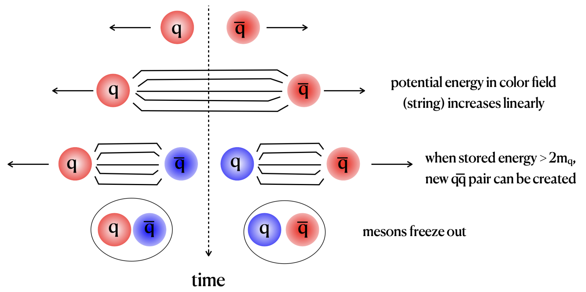
No isolated color charge has been observed in particle detectors to date. The hadronization process results in jets (cone-shaped sprays) of hadrons, which are considered to be the macroscopic manifestation of perturbative QCD. In the analysis of experimental high-energy physics data, a jet is a final-state construct introduced for the ease of interpreting the data and finding relevant signatures. Jet finding algorithms usually look for collimated sprays of particles in a cone with typical radii (with the azimuthal angle and the polar-angle related rapidity), applying purely geometrical and combinatorial considerations. Finding complete jets is difficult if the acceptance is limited and/or if the involved processes are too soft, which is why jet-analysis techniques are typically not applied at fixed-target nuclear experiments.
Appendix E Hadrons
Particles composed of quarks are called hadrons. Quarks and gluons are generically referred to as partons. The quarks inside hadrons are held together by gluons, the force carriers of the strong nuclear interaction (Sec. D.1), and they are subject to the peculiar effects of asymptotic freedom and confinement described in Sec. D.2. Typical representatives of hadrons are baryons, three-quark compounds (q ) and thus fermions, and mesons, two-quark compounds and thus bosons. Searches for exotic hadrons such as treta- or pentaquarks with four or five quarks are ongoing.
The proton is the lightest baryon with a mass of 938 MeV. The neutron is slightly heavier at around 940 MeV. Protons and neutrons are collectively called nucleons. The proton is the only stable baryon,1414 14 No proton decay has been observed to date. The proton’s lifetime as determined by experiments is currently beyond years. unless it is very close to other protons at very high temperatures such as the center of our Sun. Then a proton can transmute into a neutron. The free neutron decays with half-life time of about 10 minutes into a proton, electron and anti-electron-neutrino unless it is bound inside a nucleus. All other baryons decay into lighter baryons. One can define a baryon as “at the end of the decay chain is a proton” and a meson as “at the end of the decay chain there is no proton”. The stability of the proton is a consequence of the conservation of baryon number, see Sec. F.
There are no stable mesons. The lightest meson, the pion ,1515
15
The three pions of different electrical charge are usually grouped together:
, and has a about mass of only 140 MeV, even though it contains two of the three quarks that make up the proton with almost seven times the mass of the pion. This mass difference is a manifestation of a large fraction of hadron mass being dynamically generated (see also Sec. D.2). The kaon, , has a mass of almost 500 MeV - i.e., halfway between pion and proton and also not explainable by the bare quark masses only.
Meson number does not have to be conserved and therefore mesons can decay into leptons. In general, anything that is not forbidden in particle physics will happen. There may however be kinematically suppressed channels. Looking at a large number of decays of the same particle, the fractions for different decay channels are called branching ratios. The charged pion decays in almost 100% of the cases into a muon and (anti-)muon-neutrino, while the neutral pion decays to almost 100% into 2 photons.
Only color-neutral, “white” hadrons are detected in our particle detectors: the 3 quarks in a baryon have different colors, the triplet of which combines to “white”, and mesons are made of quark pairs of color plus anti-color, which effects to “white”.
The name “lepton” comes from the Greek word for “small” or “weak” since leptons are elementary and do not interact via the strong force. The term “hadron” was coined after the Greek word for “strong” since all hadrons are subject to the strong nuclear force (see Sec. D). “Baryon” contains the Greek word for “heavy” and “meson” that for “middle” - they are not as heavy as protons, but heavier than electrons.
E.1 The nucleon in a nutshell

The three valence quarks in the nucleon determine its quantum numbers (like electrical and color charge, baryon number, strong isospin and strangeness, and others, see Sec. F). All other quarks in the nucleon - the sea quarks - occur as quark-antiquark pairs, the creation energy for which can be “borrowed” from the vacuum for a sufficiently short time (uncertainty principle). The sea quarks’ effective quantum numbers average to zero and thus do not contribute to the nucleon’s quantum numbers. Figure E.1 represents a sketch of the nucleon’s inside with its valence quarks with three different colors, quark-antiquark pairs with color-anticolor and the gluons as yellow wavy lines. Valence quarks, sea quarks and gluons possess spin and orbital angular momentum, which contribute to the nucleon’s total angular momentum.
E.2 Three quarks for Muster Mark
The title of this subsection stems from James Joyce’s Finnegans Wake. This line inspired Murray Gell-Mann in 1964 to name the fundamental constituents of the nucleon “quarks”. Let’s take a quick walk through the exciting history of early particle physics.
With the realization in the late 19th century that “the atom” is not an elementary particle and with the identification of the electron, the proton and the neutron, the old desire of mankind to explain matter in terms of just a handful ingredients flamed up again. This hope was short lived. Once more, nature turned out to be more complex.
Electrons were first observed as cathode rays in the 1880’s, but they were not yet identified as part of the atom. Based on the Geiger–Marsden experiments carried out in 1908 and following years (Rutherford gold-foil experiments), Ernest Rutherford established the modern atomic model in 1911: the mass of the atom is concentrated in its nucleus, which is positively charged. Electrons are negatively charged and orbit the nucleus. The atom is vastly empty. Rutherford gave the proton its name because it is the nucleus of the lightest atom: “proton” comes from the Greek word for “the first”. Coining the word “neutron”, Rutherford also anticipated the existence of another proton-like, but electrically neutral particle since the masses of the investigated nuclei were larger than what would have been expected from their positive charge. Shortly after, James Chadwick experimentally identified the neutron in 1932. Together with photons (based on the Greek word for “light”), electrons, protons and neutrons had become the well-known particles of daily life. It was also known that there must be a particle that is not detected but that carries away missing energy in the radioactive beta decay, and this particle was called neutrino.
Until 1947, the situation remained relatively simple. Cosmic ray experiments using cloud chambers had revealed the existence of a few “exotic particles”: the positron (the first anti-particle), the muon (first 2nd-generation particle) and the pion (the first meson). The detection of the positron in 1933 (Carl Anderson at Caltech) was a triumph after Paul Dirac’s prediction of anti-particles from 1928. The discovery of the neutral pion in 1947 (Cecil Powell at Bristol) matched well Hideki Yukawa’s prediction from 1935 that mesons mediate the strong nuclear force. Something like such strong force should exist because otherwise the atomic nucleus would drift apart due to electrostatic repulsion between the positively charged protons. The muon had been discovered in cosmic rays already in 1937 (Carl Anderson and Seth Neddermeyer at Caltech) and was at first mistakenly identified as the Yukawa particle. Thus for every new discovery, there was a solid theoretical explanation available and the new exotic particles were not considered to be first glimpses of new physics, even though the muon did not really seem to fit in since it was not needed to explain the behavior of nuclei.
For the discovery of the pion, the usage of photographic emulsion plates at high altitudes had been essential. It then also enabled the detection of “strange particles”: the kaon (us) in 1947 and the Lambda baryon (uds) in 1950 with experimental signatures that did not fit to any of the previously discovered particles. These hadrons are usually generated via the strong interaction, but they decay via the weak interaction and they can create hadrons in their decay, even though the decay does not proceed via the strong interaction. This was considered to be strange. It was later realized that these particles contain a quark of the 2nd generation, which received the name “strange quark”. By 1960, a whole “zoo of particles” was known.
In 1961, Gell-Mann and Yuval Ne’eman realized that the hadrons could be ordered in groups, called multiplets, of 8, 9 or 10 members with zero average isospin 3-component , same hypercharge , and common spin-parity quantum number (see Sec. F), as shown in Fig. E.2. Electrical charge, strangeness and isospin are related through Eq. 128.
The three heavier quarks discovered after 1961 also found their place in the multiplet ordering scheme. The J particle was discovered in the November revolution of 1974 at Brookhaven National Lab in proton-beryllium scattering (Samuel C. C. Ting’s MIT group) and SLAC in electron-positron collisions (Burton Richter) and was later realized to be a state, with the “new” charm quark forming a duo with the so-far unpartnered s-quark. Around the same time, the heaviest lepton was found - the -lepton (Martin L. Perl and Y.-s. Tsai). The next heavier quark, the bottom quark, was found at Fermilab in 1977 in proton-copper/platinum scattering with the discovery of the particle, a state (Leon Lederman). It took almost two decades for the heaviest quark, the top quark with a mass of a gold atom, to be found at Fermilab in 1995 in proton-antiproton collisions (Tevatron CDF and D0 collaborations). A complete description of meson and baryon multiplets can, e.g., be found in the Particle Data Group’s (PDG) listings [153].
This organization scheme is sometimes called the eightfold way in allusion to the Noble Eightfold Path of Buddhism. The quark model was established in 1963 - hadrons are made of colored quarks; but hadrons are always color neutral. Nature’s order scheme and symmetry was found to be represented once more by elements of group theory: the quantum numbers of hadrons turn out to be one-to-one related to members of the special unitary Lie group SU(3). The 1969 Nobel Prize in Physics was awarded to Gell-Mann “for his contributions and discoveries concerning the classification of elementary particles and their interactions”.
Appendix F Conservation laws
Conservation laws are based off symmetries we find in nature. The Emmy-Noether theorem teaches us that when there exists a symmetry transformation that does not change the Lagrange function, there is a corresponding conserved quantity. Examples are: space and time are homogeneous, i.e., there is translational invariance, and it follows that momentum is conserved; space is isotropic, i.e., there is rotational invariance, and it follows angular momentum is conserved. Table F.1 gives an overview over conserved quantities that are essential for particle physics.
| symbol | name | elmag? | weak? | strong? | anti-particle remarks |
| Q | electrical | charged anti-particles have | |||
| charge | opposite-sign charge | ||||
| r,g,b | color | anti-hadrons: | |||
| charge | coloranti-color | ||||
| baryon | for baryons, | ||||
| number | for anti-baryons | ||||
| lepton | |||||
| generation | ↯ | for leptons & | |||
| number | for anti-leptons | ||||
| strangeness | ↯ | -quark: , | |||
| anti--quark: | |||||
| strong | isospin n-tuplets contain | ||||
| isospin | their anti-particles | ||||
| weak | see remark for | ||||
| isospin | |||||
| parity | ↯ | particle and anti-particle | |||
| have opposite parity | |||||
| charge | ↯ | is the anti-particle operator | |||
| conjugation | also for neutral particles | ||||
| charge conj. | (↯) | makes anti-particle | |||
| & parity | & mirrors | ||||
| & time- | makes anti-particle, | ||||
| reversal | mirrors & reverses time |
F.1 Particle types
The lepton generation number is not conserved when neutrinos oscillate between flavors (see Sec. C). Charged leptons have not been observed to violate lepton-generation number conservation. In the weak interaction, strangeness changes by or . Similarly, also the quantum numbers related to charm (), bottom (bottomness ), and top (topness ) flavors are preserved under the strong and electromagnetic interactions, but not under weak interaction. The hypercharge ,
| (120) |
and the weak hypercharge ,
| (121) |
are conserved in the strong, but not in the weak interaction. Another way of thinking about strangeness conservation is that spin flips can happen fast (e.g., the strong decay , effectively ), while changing the quark generation takes a longer time (e.g., the weak decay , , with strangeness non-conservation).
F.2 Angular momentum and isospin
Orbital angular momentum, spin, and isospin obey the same angular momentum algebra. With the generic angular momentum operator and its 3-component , one has the Lie algebra
| (122) |
from which the quantization of angular momentum in the microscopic world can be derived. Because and commute, , they have common eigenvectors forming the eigenstates of angular momentum with eigenvalues and :
| (123) | |||||
| (124) |
The algebra of angular momentum is described by the special unitary Lie group SU(2), which is generated by anti-Hermitian, trace-zero matrices, the Pauli spin matrices , and :
| (125) |
The elements of SU(2) rotate one eigenstate into another:
| (126) |
A prominent example of a quantity following algebra Eqs. 122-126 is the particle’s spin, sometimes called “intrinsic angular momentum”.
Isospin is a spin-like quantum number obeying angular momentum algebra with eigenvalues ( from Eq. 123) and ( from Eq. 124). Since can take values between and , there are in total possibilities. Historically, isospin was introduced to classify those hadrons that behave identical under the strong interaction into a multiplet with multiplicity , for example:
| (127) |
Initially called “isotopic spin”, the name isospin can be explained as defining those particles that take the “same location” (isotopic in Greek), in analogy to the isotopes in the periodic table of elements. What is “same number of protons” there, is “same isospin” here. One “obtains a neutron by rotating a proton in isospin space” (the in Eq. 126). Maybe best understood can isospin be in when considering that u-quarks have and d-quarks , which is where they have their names from - “isospin up” and “isospin down”. The quarks of heavier flavors (s, c, b, t) have , while each carrying their own quantum number, for example strangeness . Not only isospin, also strangeness, the other “flavornesses”, and parity are important for the classification scheme of hadrons into multiplets (see also Sec. E.2). The Gell-Mann–Nishijima formula relates isospin, electrical charge and strangeness:
| (128) |
At applicable center-of-mass energies, the heavier flavors have to be added as spelled out in the hypercharge in Eq. 120.
While was above introduced as generic angular momentum, it usually denotes the total angular momentum of a particle , with its spin1616 16 Here denoted with a small to avoid confusion with strangeness and the orbital angular momentum. We have found an example of the coupling of two angular momenta. Couplings between spin and orbital angular momentum are called spin-orbit couplings. For example, the electrons’ spin-orbit coupling creates the atom’s fine structure in the shell of the hydrogen atom.
The spin-parity quantum number used to classify particles is introduced in Sec. F.3.
F.3 Parity, charge conjugation and time reversal
We define the helicity of a particle, with its 3-momentum vector and its spin vector:
| (129) |
and will now take a closer look at three fundamental symmetry operations:
-
Parity . The operation that “mirrors” (changes the sign) of polar vectors (e.g., position and momentum vectors) and pseudo scalars (e.g., helicity, see Eq. 129), and leaves unchanged axial vectors1717 17 Axial vectors are vectors that point in the direction of a rotational axis, i.e., that have a sense of left and right - “a right-hand helix stays a right-hand helix” (e.g., angular momentum, magnetic field); the vector product of two same-kind vectors (polar polar or axial axial) is an axial vector, otherwise polar. (e.g., angular momentum ) and scalars.1818 18 e.g., numbers of things, densities, etc. means even and odd parity. Every particle has its intrinsic parity: photons ; mesons ; baryons . One bulk defines a particle’s quantum numbers using the notation , with the total angular momentum from Sec. F.2, or even (see next item for ). For example, for the photon and for the meson .
-
Charge conjugation . The operation that changes the sign of all electrically charged particles. Effectively, it turns a particle into its anti-particle: . All charge-like quantum numbers are changed (also lepton and baryon number). As , is a discrete symmetry and multiplicative.
-
Time reversal . The operation that reverses the time arrow of the reaction. For example, the direction of momentum, orbital angular momentum, spin, and magnetic field vectors is reversed. The direction of, e.g., position, force, and electric field vectors is conserved under .
The weak interaction violates parity symmetry , often written as “”. When we say that a process violates parity, we mean that the process looks differently in a mirror image of the universe.
In 1957, Chien-Shiung Wu (Madame Wu) studied the radioactive beta decay1919 19 On nucleon level: ; on quark level: of 60Co atoms to 60Ni. Her experimental finding was that the decay electrons are emitted preferably against the magnetic field direction. Together with total angular momentum conservation, one can conclude that electrons are always left-handed (negative helicity, see Eq. 129) and anti-neutrinos always right-handed (positive helicity).2020 20 Here, the mass of the electron is neglected and it is assumed to travel at . Particles with mass can have the wrong helicity, like the right-handed muons from the pion decay (Fig. 3.3). Because of the smallness of the electron mass, the pion decay into electrons is suppressed. Any interaction that is parity conserving should equally couple to left- and right-handed particles. The weak interaction for charged currents (CC) is maximally parity violating. The W± couple only to left-handed fermions and right-handed anti-fermions. The Z0 however (neutral weak current NC) couples also to right-handed fermions (partial parity violation), which is a manifestation of the close relation between the Z0 and the photon in electroweak unification.
Also the charge symmetry is broken in the weak interaction. What about the combined charge and parity symmetry, , i.e., exchanging all particles with their anti-particles while also also looking at the mirrored situation? A left-handed fermion is turned by into a right-handed anti-fermion. There are no other combinations than left-handed fermion or right-handed anti-fermion, and is the symmetry operation between them. The symmetry is conserved in all interactions including the electromagnetic and strong interaction. An exception is the weak interaction, but only for weak neutral K-meson decays ( / ) and for the weak B-meson sector, where the combined symmetry is violated (). If a -violating reaction is looked at under time-reversed arrow, the symmetry is restored. The three-fold symmetry is considered a fundamental property of physical laws.
F.4 The weak force
Examination of Tab. F.1 aids in understanding why the weak nuclear force is sometimes referred to as “the force of change”. Not only can it change one form of particle into another - a nucleus of one chemical element into the nucleus of a different element, or a neutron into a proton, or a meson into a lepton, and others - but also does the weak force not preserve some of the quantities and symmetries that are conserved by all other forces (including gravity, which is not listed in the table). One other prominent feature of the weak force is its slowness (see Tab. D.1), which it owes its name to. If it weren’t for the slow burning of our Sun’s nuclear oven, a process that is driven by the weak process transmuting at high temperatures and high densities a proton into a neutron to form deuteron, a heavy hydrogen nucleus, pp , you would not be reading this - the Sun would have run out of hydrogen “fuel” a long time ago.
Appendix G Nobel Prizes in Physics related to particle physics
Figure G.1 shows the number of particle-physics-related Nobel Prizes in Physics per decade that were awarded for achievements in the theory sector, novel instrumentation, or major collaborative experimental efforts. For the early years, also general achievements are counted that were essential for particle physics.
For more information on each prize, visit the Nobel Prize official web page.2121 21 At https://www.nobelprize.org/prizes/physics/XXXX/summary, where XXXX is the 4-digit year number The laureates and their achievements are:
-
2015 to Takaaki Kajita and Arthur B. McDonald “for the discovery of neutrino oscillations, which shows that neutrinos have mass”
-
2013 to Francois Englert and Peter W. Higgs “for the theoretical discovery of a mechanism that contributes to our understanding of the origin of mass of subatomic particles, and which recently was confirmed through the discovery of the predicted fundamental particle, by the ATLAS and CMS experiments at CERN’s Large Hadron Collider"
-
2008 to Yoichiro Nambu “for the discovery of the mechanism of spontaneous broken symmetry in subatomic physics” and
to Makoto Kobayashi and Toshihide Maskawa “for the discovery of the origin of the broken symmetry which predicts the existence of at least three families of quarks in nature”
-
2004 David J. Gross, H. David Politzer and Frank Wilczek “for the discovery of asymptotic freedom in the theory of the strong interaction”
-
2002 to Raymond Davis Jr. and Masatoshi Koshiba “for pioneering contributions to astrophysics, in particular for the detection of cosmic neutrinos” and
to Riccardo Giacconi “for pioneering contributions to astrophysics, which have led to the discovery of cosmic X-ray sources”
-
1999 to Gerardus ‘t Hooft and Martinus J.G. Veltman “for elucidating the quantum structure of electroweak interactions in physics”
-
1995 “for pioneering experimental contributions to lepton physics”
to Martin L. Perl “for the discovery of the tau lepton” and
to Frederick Reines “for the detection of the neutrino”
-
1992 to Georges Charpak “for his invention and development of particle detectors, in particular the multiwire proportional chamber”
-
1990 to Jerome I. Friedman, Henry W. Kendall and Richard E. Taylor “for their pioneering investigations concerning deep inelastic scattering of electrons on protons and bound neutrons, which have been of essential importance for the development of the quark model in particle physics”
-
1988 to Leon M. Lederman, Melvin Schwartz and Jack Steinberger “for the neutrino beam method and the demonstration of the doublet structure of the leptons through the discovery of the muon neutrino”
-
1984 to Carlo Rubbia and Simon van der Meer “for their decisive contributions to the large project, which led to the discovery of the field particles W and Z, communicators of weak interaction”
-
1980 to James Watson Cronin and Val Logsdon Fitch “for the discovery of violations of fundamental symmetry principles in the decay of neutral K-mesons”
-
1976 to Burton Richter and Samuel Chao Chung Ting “for their pioneering work in the discovery of a heavy elementary particle of a new kind”
-
1979 to Sheldon Lee Glashow, Abdus Salam and Steven Weinberg “for their contributions to the theory of the unified weak and electromagnetic interaction between elementary particles, including, inter alia, the prediction of the weak neutral current”
-
1969 to Murray Gell-Mann “for his contributions and discoveries concerning the classification of elementary particles and their interactions”
-
1968 to Luis Walter Alvarez “for his decisive contributions to elementary particle physics, in particular the discovery of a large number of resonance states, made possible through his development of the technique of using hydrogen bubble chamber and data analysis”
-
1965 to Sin-Itiro Tomonaga, Julian Schwinger and Richard P. Feynman “for their fundamental work in quantum electrodynamics, with deep-ploughing consequences for the physics of elementary particles”
-
1963 to Eugene Paul Wigner “for his contributions to the theory of the atomic nucleus and the elementary particles, particularly through the discovery and application of fundamental symmetry principles” and
to Maria Goeppert Mayer and J. Hans D. Jensen “for their discoveries concerning nuclear shell structure”
-
1961 to Robert Hofstadter “for his pioneering studies of electron scattering in atomic nuclei and for his thereby achieved discoveries concerning the structure of the nucleons” and
to Rudolf Ludwig Moessbauer “for his researches concerning the resonance absorption of gamma radiation and his discovery in this connection of the effect which bears his name”
-
1960 to Donald Arthur Glaser “for the invention of the bubble chamber”
-
1959 to Emilio Gino Segre and Owen Chamberlain “for their discovery of the antiproton”
-
1958 to Pavel Alekseyevich Cherenkov, Il’ja Mikhailovich Frank and Igor Yevgenyevich Tamm “for the discovery and the interpretation of the Cherenkov effect”
-
1957 to Chen Ning Yang and Tsung-Dao (T.D.) Lee “for their penetrating investigation of the so-called parity laws which has led to important discoveries regarding the elementary particles”
-
1950 to Cecil Frank Powell “for his development of the photographic method of studying nuclear processes and his discoveries regarding mesons made with this method”
-
1949 to Hideki Yukawa “for his prediction of the existence of mesons on the basis of theoretical work on nuclear forces”
-
1948 to Patrick Maynard Stuart Blackett “for his development of the Wilson cloud chamber method, and his discoveries therewith in the fields of nuclear physics and cosmic radiation”
-
1945 to Wolfgang Pauli “for the discovery of the Exclusion Principle, also called the Pauli Principle”
-
1939 to Ernest Orlando Lawrence “for the invention and development of the cyclotron and for results obtained with it, especially with regard to artificial radioactive elements”
-
1936 to Victor Franz Hess “for his discovery of cosmic radiation” and
to Carl David Anderson “for his discovery of the positron”
-
1935 to James Chadwick “for the discovery of the neutron”
-
1933 to Erwin Schrödinger and Paul Adrien Maurice Dirac “for the discovery of new productive forms of atomic theory”
-
1932 to Werner Karl Heisenberg “for the creation of quantum mechanics, the application of which has, inter alia, led to the discovery of the allotropic forms of hydrogen”
-
1927 to Arthur Holly Compton “for his discovery of the effect named after him” and
to Charles Thomson Rees Wilson “for his method of making the paths of electrically charged particles visible by condensation of vapour”
-
1922 to Niels Henrik David Bohr “for his services in the investigation of the structure of atoms and of the radiation emanating from them”
-
1921 to Albert Einstein “for his services to Theoretical Physics, and especially for his discovery of the law of the photoelectric effect”
-
1918 to Max Karl Ernst Ludwig Planck “in recognition of the services he rendered to the advancement of Physics by his discovery of energy quanta”
-
1903 to Antoine Henri Becquerel “in recognition of the extraordinary services he has rendered by his discovery of spontaneous radioactivity” and
to Pierre Curie and Marie Curie, nee Sklodowska “in recognition of the extraordinary services they have rendered by their joint researches on the radiation phenomena discovered by Professor Henri Becquerel”
References
- [1] EMC Collaboration, A measurement of the spin asymmetry and determination of the structure function in deep inelastic muon-proton scattering, Phys. Lett. B 206 (1988) 364-370, 10.1016/0370-2693(88)91523-7.
- [2] A. Jaffe, Where Does the Proton Really Get Its Spin?, Physics Today 48, 9, 24 (1995), 10.1063/1.881473.
- [3] B. Povh, K. Rith, C. Scholz, F. Zetsche, Particles and Nuclei, Springer (2006), ISBN 9783540366843.
- [4] J. B. Bellicard, P. Bounin, R. F. Frosch, R. Hofstadter, J. S. McCarthy, F. J. Uhrhane, M. R. Yearian, B. C. Clark, R. Herman, and D. G. Ravenhall, Scattering of 750-MeV Electrons by Calcium Isotopes, Phys. Rev. Lett. 19, 527 (1967), 10.1103/PhysRevLett.19.527.
- [5] Muon g-2 Collaboration, Measurement of the Positive Muon Anomalous Magnetic Moment to 0.46 ppm, Phys. Rev. Lett. 126, 141801 (2021), 10.1103/PhysRevLett.126.141801.
- [6] W. Bartel, B. Dudelzak, H. Krehbiel, J. McElroy, U. Meyer-Berkhout, W. Schmidt, V. Walther, G. Weber, Electroproduction of pions near the isobar and the form factor of the ()-vertex, Phys. Lett. B 28, 148-151 (1968), 10.1016/0370-2693(68)90155-X.
- [7] W. B. Atwood, Lepton Nucleon Scattering, Lecture given at the SLAC summer institute on particle physics: Quantum Chromodynamics, July 9-20, 1979, SLAC-PUB-2428.
- [8] R. E. Taylor, The Discovery of the Point-Like Structure of Matter, Invited talk presented at the Discussion Meeting on the Quark Structure of Matter, Royal Society of London, England, May 24–25, 2000, SLAC-PUB-8640.
- [9] F. Close, The quark parton model, Rep. Prog. Phys. 42, 1285 (1979).
- [10] HERMES Collaboration, Inclusive measurements of inelastic electron and positron scattering from unpolarized hydrogen and deuterium targets, J. High Energ. Phys. 2011, 126 (2011), 10.1007/JHEP05(2011)126.
- [11] R. Abdul Khalek, A. Accardi, J. Adam, D. Adamiak, W. Akers, M. Albaladejo, A. Al-bataineh, M. G. Alexeev, F. Ameli and P. Antonioli, et al., Science Requirements and Detector Concepts for the Electron-Ion Collider: EIC Yellow Report, [arXiv:2103.05419 [physics.ins-det]].
- [12] G. Altarelli and G. Parisi, Asymptotic freedom in parton language, Nucl. Phys. B 126, 298-318 (1977), 10.1016/0550-3213(77)90384-4.
- [13] R. Klanner and T. Schörner-Sadenius, Verstehen wir die starke Kraft? (“Do we understand the strong interaction?”), Physik Journal 5 (2006) Nr. 5.
- [14] H1 and ZEUS Collaborations, Combination of measurements of inclusive deep inelastic scattering cross sections and QCD analysis of HERA data, Eur. Phys. J. C 75, 580 (2015), 10.1140/epjc/s10052-015-3710-4.
- [15] M. Klein, R. Yoshida, Collider physics at HERA, Prog. Part. Nucl. Phys. 61 343-393 (2008), 10.1016/j.ppnp.2008.05.002.
- [16] ATLAS Collaboration, Determination of the parton distribution functions of the proton using diverse ATLAS data from pp collisions at 7, 8 and 13 TeV, arXiv:2112.11266, submitted to EPJC.
- [17] NMC Collaboration, The ratio in deep inelastic muon scattering, Nucl. Phys. B 371 (1992) 3, 10.1016/0550-3213(92)90227-3.
- [18] NMC Collaboration, Reevaluation of the Gottfried sum, Phys. Rev. D 50, R1(R) (1994), 10.1103/PhysRevD.50.R1.
- [19] J.-C. Peng and G. T. Garvey, Flavor asymmetry of the sea quark distributions, arXiv:hep-ph/9912370v2.
- [20] J. Dove, B. Kerns, R.E. McClellan et al. (SeaQuest Collaboration), The asymmetry of antimatter in the proton, Nature 590, 561–565 (2021), 10.1038/s41586-021-03282-z.
- [21] STAR Collaboration, Measurements of and cross sections and their ratios in collisions at RHIC, Phys. Rev. D 103, 012001 (2021), 10.1103/PhysRevD.103.012001.
- [22] D. H. Perkins, Neutrino interactions, in Proceedings, XVI International Conference on High-Energy Physics, University of Chicago, 6 to 13 September 1972, J. D. Jackson and A. Roberts, Eds. (Fermi National Accelerator Laboratory, Batavia, IL, 1972), vol. 4, p. 189.
- [23] J. I. Friedman, Deep Inelastic Scattering: Comparisons with the Quark Model, Nobel Lecture, December 8, 1990.
- [24] M. Riordan, The Discovery of Quarks, Science 256, no. 5061 (1992), 1287–93.
- [25] C. W. Leemann, D. R. Douglas, G.A. Krafft, The continuous electron beam accelerator facility: BEBAF at the Jefferson Laboratory, Annu. Rev. Nucl. Part. Sci. 51 413–50 (2001), 10.1146/annurev.nucl.51.101701.132327.
- [26] I. Alekseev, C. Allgower, M. Bai, et al., Polarized proton collider at RHIC, Nucl. Inst. Meth. A 499 392-414 (2003),10.1016/S0168-9002(02)01946-0.
- [27] D.P. Barber, H.-D. Bremer, M. Böge, et al., The HERA polarimeter and the first observation of electron spin polarization at HERA, Nucl. Inst. Meth. A 329 79-111 (1993),10.1016/0168-9002(93)90924-7.
- [28] D.P. Barber, M. Böge, H. Böttcher, H.-D. Bremer, R. Brinkmann, W. Brückner, M. Düren, E. Gianfelice-Wendt, R. Kaiser, R. Klanner, H.-Ch. Lewin, M. Lomperski, N. Meyners, W.-D. Nowak, P.M. Patel, G. Ripken, K. Rith, H.O. Roloff, E. Steffens, D. Westphal, K. Zapfe, F. Zetsche, High spin polarization at the HERA electron storage ring, Nucl. Inst. Meth. A338 166-184 (1994), 10.1016/0168-9002(94)91311-0.
- [29] HERMES Collaboration, Quark helicity distributions in the nucleon for up, down, and strange quarks from semi-inclusive deep-inelastic scattering, Phys. Rev. D 71, 012003 (2005), 10.1103/PhysRevD.71.012003.
- [30] C. Riedl and HERMES Collaboration, Positrons and Electrons at HERA and HERMES , AIP Conference Proceedings 1160, 36 (2009), 10.1063/1.3232030.
- [31] J. Bernhard, D. Banerjee, E. Montbarbon, M. Brugger, N. Charitonidis, S. Cholak, G. Luigi D’Alessandro, L. Gatignon, A. Gerbershagen, B. Rae, M. Rosenthal, M. van Dijk, B. M. Veit, Studies for New Experiments at the CERN M2 Beamline within “Physics Beyond Colliders”: AMBER/COMPASS++, NA64mu, MuonE, arXiv:1911.01498 [hep-ex].
- [32] J.H. Koivuniemi, A. Berlin, F. Gautheron, W. Meyer, G. Reicherz, N. Doshita, T. Iwata, K. Kondo, G. Nukazuka, J. Matousek, M. Pesek, Y. Kisselev and M. Finger, Large COMPASS polarized solid state target for Drell-Yan physics, PoS PSTP2015 (2015) 015, 10.22323/1.243.0015.
- [33] HERMES Collaboration, The HERMES polarized hydrogen and deuterium gas target in the HERA electron storage ring, Nucl. Inst. Meth. A 540 68-101 (2005), 10.1016/j.nima.2004.11.020.
- [34] C.D. Keith, J. Brock, C. Carlin, S.A. Comer, D. Kashy, J. McAndrew, D.G. Meekins, E. Pasyuk, J.J. Pierce and M.L. Seely, The Jefferson Lab frozen spin target, Nucl. Inst. Meth. A 684 27-35 (2012), 10.1016/j.nima.2012.04.067.
- [35] SpinQuest Collaboration, Probing nucleon’s spin structures with polarized Drell-Yan in the Fermilab SpinQuest experiment, arXiv:1901.09994v2 [nucl-ex].
- [36] P. Lenisa, E. Steffens, V. Carassiti, G. Ciullo, P. Di Nezza, L. Pappalardo, A. A. Vasilyev, LHCspin: a polarized internal target for the LHC, PoS PSTP2019 (2020) 025, 10.22323/1.379.0025.
- [37] St. Goertz, W. Meyer, G. Reicherz, Polarized H, D and 3He targets for particle physics experiments, Prog. Part. Nucl. Phys. 49 403-489 (2002), 10.1016/S0146-6410(02)00159-X.
- [38] HERMES Collaboration, Precise determination of the spin structure function g1 of the proton, deuteron, and neutron, Phys. Rev. D 75, 012007 (2007), 10.1103/PhysRevD.75.012007.
- [39] COMPASS Collaboration, The spin structure function of the proton and a test of the Bjorken sum rule, Phys. Lett. B 753, 18-28 (2016), 10.1016/j.physletb.2015.11.064.
- [40] COMPASS Collaboration, Final COMPASS results on the deuteron spin-dependent structure function and the Bjorken sum rule, Phys. Lett. B 769, 34-41 (2017),10.1016/j.physletb.2017.03.018.
- [41] COMPASS Collaboration, Longitudinal double-spin asymmetry and spin-dependent structure function of the proton at small values of and , Phys. Lett. B 781, 464-472 (2018), 10.1016/j.physletb.2018.03.044.
- [42] B. Badelek, Final COMPASS results on the spin-dependent structure functions and in the deep-inelastic and nonperturbative regions, PoS DIS2017 (2018) 247, 10.22323/1.297.0247.
- [43] J. D. Bjorken, Applications of the Chiral Algebra of Current Densities, Phys. Rev. 148, 1467 (1966), doidoi.org/10.1103/PhysRev.148.1467.
- [44] D. de Florian, R. Sassot, M. Stratmann, and W. Vogelsang, Extraction of spin-dependent parton densities and their uncertainties, Phys. Rev. D 80, 034030 (2009), 10.1103/PhysRevD.80.034030.
- [45] J. Allison, K. Amako, J. Apostolakis, et al., Recent developments in Geant4, Nucl. Inst. Meth. A 835, 186-225 (2016), 10.1016/j.nima.2016.06.125.
- [46] HERMES Collaboration, Erratum to: “Nuclear effects on in deep-inelastic scattering”: [Phys. Lett. B 475 (2000) 386–394], Phys. Lett. B 567, 339-346 (2003), 10.1016/j.physletb.2003.06.044.
- [47] P. Hoodbhoy, R.L. Jaffe, A Manohar, Novel effects in deep inelastic scattering from spin-one hadrons, Nucl. Phys. B 312, 571-588 (1989), 10.1016/0550-3213(89)90572-5.
- [48] M. E. Peskin and D.V. Schroeder, An Introduction to quantum field theory, Addison-Wesley (1995), ISBN 9780201503975.
- [49] HERMES Collaboration, Measurement of the Tensor Structure Function of the Deuteron, Phys. Rev. Lett. 95, 242001 (2005), 10.1103/PhysRevLett.95.242001.
- [50] C. Riedl, The first measurement of the tensor structure function of the deuteron with the HERMES experiment, PhD thesis, University of Erlangen-Nuremberg (2005), 10.3204/DESY-THESIS-2005-027.
- [51] K. Rith, Spin asymmetries in deep-inelastic electron-nucleon scatering - selected HERMES results, Prog. Part. Nucl. Phys 49 (2002) 245-324, 10.1016/S0146-6410(02)00157-6.
- [52] COMPASS Collaboartion, Flavour separation of helicity distributions from deep inelastic muon–deuteron scattering, Phys. Lett. B 680, 217-224 (2009), 10.1016/j.physletb.2009.08.065.
- [53] D. de Florian, R. Sassot, and M. Stratmann, Global analysis of fragmentation functions for pions and kaons and their uncertainties, Phys. Rev. D 75, 114010 (2007), 10.1103/PhysRevD.75.114010.
- [54] HERMES Collaboration, Longitudinal double-spin asymmetries in semi-inclusive deep-inelastic scattering of electrons and positrons by protons and deuterons, Phys. Rev. D 99, 112001 (2019), 10.1103/PhysRevD.99.112001.
- [55] CLAS Collaboration, Measurement of Single- and Double-Spin Asymmetries in Deep Inelastic Pion Electroproduction with a Longitudinally Polarized Target, Phys. Rev. Lett. 105, 262002 (2010), 10.1103/PhysRevLett.105.262002.
- [56] STAR Collaboration, Measurement of the longitudinal spin asymmetries for weak boson production in proton-proton collisions at GeV, Phys. Rev. D 99, 051102(R) (2019), 10.1103/PhysRevD.99.051102.
- [57] PHENIX Collaboration, Cross section and longitudinal single-spin asymmetry for forward production in polarized collisions at GeV, Phys. Rev. D 98, 032007 (2018), 10.1103/PhysRevD.98.032007.
- [58] E. R. Nocera, R. D. Ball, S. Forte, G. Ridolfi, J. Rojo (NNPDF Collaboration), A first unbiased global determination of polarized PDFs and their uncertainties, Nucl. Phys. B 887, 276-308 (2014), 10.1016/j.nuclphysb.2014.08.008.
- [59] PHENIX Collaboration, Measurement of charged pion double spin asymmetries at midrapidity in longitudinally polarized collisions at GeV, Phys. Rev. D 102, 032001 (2020), 10.1103/PhysRevD.102.032001.
- [60] STAR Collaboration, Longitudinal double-spin asymmetry for inclusive jet and dijet production in polarized proton collisions at GeV, Phys. Rev. D 103, L091103 (2021), 10.1103/PhysRevD.103.L091103.
- [61] HERMES Collaboration, Leading-order determination of the gluon polarization from high-p T hadron electroproduction J. High Energ. Phys. 2010, 130 (2010), 10.1007/JHEP08(2010)130.
- [62] COMPASS Collaboration, Leading-order determination of the gluon polarisation from semi-inclusive deep inelastic scattering data, Eur. Phys. J. C 77, 209 (2017), 10.1140/epjc/s10052-017-4716-x.
- [63] M. Diehl, Introduction to GPDs and TMDs, Eur. Phys. J. A 52, 149 (2016), 10.1140/epja/i2016-16149-3.
- [64] E. Aschenauer, S. Fazio, K. Kumerički, D. Mueller, Deeply virtual Compton scattering at a proposed high-luminosity Electron-Ion Collider, J. High Energ. Phys. 2013, 93 (2013), 10.1007/JHEP09(2013)093.
- [65] A.V. Belitsky, D. Mueller, Nucleon hologram with exclusive leptoproduction, Nucl. Phys. A 711, 118-126 (2002), 10.1016/S0375-9474(02)01202-2.
- [66] HERMES Collaboration, Measurement of the Beam-Spin Azimuthal Asymmetry Associated with Deeply-Virtual Compton Scattering, Phys. Rev. Lett. 87, 182001 (2001), 10.1103/PhysRevLett.87.182001.
- [67] CLAS Collaboration, Observation of Exclusive Deeply Virtual Compton Scattering in Polarized Electron Beam Asymmetry Measurements, Phys. Rev. Lett. 87, 182002 (2001), 10.1103/PhysRevLett.87.182002.
- [68] HERMES Collaboration, Beam-helicity and beam-charge asymmetries associated with deeply virtual Compton scattering on the unpolarised proton, JHEP 07 (2012) 032, 10.1007/JHEP07(2012)032.
- [69] HERMES Collaboration, Measurement of azimuthal asymmetries associated with deeply virtual Compton scattering on an unpolarized deuterium target, Nucl. Phys. B 829 1-27 (2010), 10.1016/j.nuclphysb.2009.12.004.
- [70] HERMES Collaboration, Beam-helicity asymmetry arising from deeply virtual Compton scattering measured with kinematically complete event reconstruction, JHEP 10 (2012) 042, 10.1007/JHEP10(2012)042.
- [71] HERMES Collaboration, Measurement of azimuthal asymmetries with respect to both beam charge and transverse target polarization in exclusive electroproduction of real photons, JHEP 06 (2008) 066, 10.1088/1126-6708/2008/06/066.
- [72] HERMES Collaboration, Measurement of double-spin asymmetries associated with deeply virtual Compton scattering on a transversely polarized hydrogen target, Phys. Lett. B 704 15-23 (2011), 10.1016/j.physletb.2011.08.067.
- [73] HERMES Collaboration, Exclusive leptoproduction of real photons on a longitudinally polarised hydrogen target, JHEP 06 (2010) 019, 10.1007/JHEP06(2010)019.
- [74] HERMES Collaboration, Measurement of azimuthal asymmetries associated with deeply virtual Compton scattering on a longitudinally polarized deuterium target, Nucl. Phys. B 842 265-298 (2011), 10.1016/j.nuclphysb.2010.09.010.
- [75] CLAS Collaboration, Single and double spin asymmetries for deeply virtual Compton scattering measured with CLAS and a longitudinally polarized proton target, Phys. Rev. D 91, 052014 (2015), 10.1103/PhysRevD.91.052014.
- [76] CLAS Collaboration, Longitudinal Target-Spin Asymmetries for Deeply Virtual Compton Scattering, Phys. Rev. Lett. 114, 032001 (2015), 10.1103/PhysRevLett.114.032001.
- [77] H1 Collaboration, Deeply virtual Compton scattering and its beam charge asymmetry in collisions at HERA, Phys. Lett. B 681, 391-399 (2009), 10.1016/j.physletb.2009.10.035.
- [78] X. Ji, Phys. Rev. Lett. 78, 610 (1997), 10.1103/PhysRevLett.78.610.
- [79] Jefferson Lab Hall A Collaboration, Deeply Virtual Compton Scattering off the Neutron, Phys. Rev. Lett. 99, 242501 (2007), 10.1103/PhysRevLett.99.242501.
- [80] W. Schmidke for the STAR Collaboration, Production in Ultra-Peripheral Heavy-Ion Collisions at STAR, talk given at the XXVIII International Workshop on Deep-Inelastic Scattering and Related Subjects (DIS21), Stony Brook (NY), USA, April 2021.
- [81] M. Burkardt, Impact Parameter Space Interpretation for Generalized Parton Distributions, Int. J. Mod. Phys. A 18, 173-208 (2003), 10.1142/S0217751X03012370.
- [82] COMPASS Collaboration, Transverse extension of partons in the proton probed in the sea-quark range by measuring the DVCS cross section, Phys. Lett. B793, 188-194 (2019), 10.1016/j.physletb.2019.04.038.
- [83] CLAS Collaboration, Measurement of deeply virtual Compton scattering off Helium-4 with CLAS at Jefferson Lab, Phys. Rev. C 104, 025203 (2021), 10.1103/PhysRevC.104.025203.
- [84] P. Chatagnon and CLAS Collaboration, 2020 J. Phys.: Conf. Ser. 1643 012185.
- [85] COMPASS Collaboration, Transverse target spin asymmetries in exclusive muoproduction, Phys. Lett. B 731, 19-26 (2014), 10.1016/j.physletb.2014.02.005.
- [86] HERMES Collaboration, Single-spin azimuthal asymmetry in exclusive electroproduction of mesons on transversely polarized protons, Phys. Lett. B 682, 345-350 (2010), /10.1016/j.physletb.2009.11.039.
- [87] HERMES Collaboration, Transverse-target-spin asymmetry in exclusive -meson electroproduction, Eur. Phys. J. C (2015) 75: 600, 10.1140/epjc/s10052-015-3825-7.
- [88] COMPASS Collaboration, Measurement of the cross section for hard exclusive muoproduction on the proton, Phys. Lett. B 805, 135454 (2020), 10.1016/j.physletb.2020.135454.
- [89] HERMES Collaboration, Spin density matrix elements in exclusive electroproduction on 1H and 2H targets at 27.5 GeV beam energy, Eur. Phys. J. C (2014) 74: 3110, 10.1140/epjc/s10052-014-3110-1.
- [90] COMPASS Collaboration, Spin density matrix elements in exclusive meson muoproduction, Eur. Phys. J. C 81, 126 (2021), 10.1140/epjc/s10052-020-08740-y.
- [91] S. V. Goloskokov, P. Kroll, The pion pole in hard exclusive vector-meson leptoproduction, Eur. Phys. J. A (2014) 50: 146, 10.1140/epja/i2014-14146-2.
- [92] CLAS Collaboration, Extraction of Beam-Spin Asymmetries from the Hard Exclusive Channel off Protons in a Wide Range of Kinematics, Phys. Rev. Lett. 125, 182001 (2020), 10.1103/PhysRevLett.125.182001.
- [93] M. Benali, C. Desnault, M. Mazouz, et al., Deeply virtual Compton scattering off the neutron, Nat. Phys. 16, 191-198 (2020), 10.1038/s41567-019-0774-3.
- [94] P. Kroll, H. Moutarde, F. Sabatie, From hard exclusive meson electroproduction to deeply virtual Compton scattering, Eur. Phys. J. C (2013) 73: 2278, 10.1140/epjc/s10052-013-2278-0.
- [95] V.D. Burkert, L. Elouadrhiri, and F.X. Girod, The pressure distribution inside the proton, Nature 557, 396–399 (2018), 10.1038/s41586-018-0060-z.
- [96] H. Moutarde, P. Sznajder, J. Wagner, Border and skewness functions from a leading order fit to DVCS data, Eur. Phys. J. C (2018) 78: 890, 10.1140/epjc/s10052-018-6359-y.
- [97] A. Accardi, J.L. Albacete, M. Anselmino, et al., Electron-Ion Collider: The next QCD frontier, Eur. Phys. J. A 52, 268 (2016), 10.1140/epja/i2016-16268-9.
- [98] M. Anselmino, M. Boglione, U. D’Alesio, S. Melis, F. Murgia, A. Prokudin, New insight on the Sivers transverse momentum dependent distribution function, J. Phys.: Conf. Ser. 295 012062 (2011), 10.1088/1742-6596/295/1/012062.
- [99] M. Anselmino, A. Mukherjee, A. Vossen, Transverse spin effects in hard semi-inclusive collisions, Prog. Part. Nucl. Phys. 114 103806 (2020), 10.1016/j.ppnp.2020.103806.
- [100] A. Bacchetta, M. Diehl, K. Goeke, A. Metz, P. J. Mulders, M. Schlegel, Semi-inclusive deep inelastic scattering at small transverse momentum, JHEP 02 (2007) 093, 10.1088/1126-6708/2007/02/093.
- [101] J. Collins, Fragmentation of transversely polarized quarks probed in transverse momentum distributions, Nucl. Phys. B 396, 161-182 (1993), 10.1016/0550-3213(93)90262-N.
- [102] S. J. Brodsky, D. S. Hwang, I. Schmidt, Final-state interactions and single-spin asymmetries in semi-inclusive deep inelastic scattering, Phys. Lett. B 530, 99-107 (2002), 10.1016/S0370-2693(02)01320-5.
- [103] HERMES Collaboration, Observation of the Naive- -Odd Sivers Effect in Deep-Inelastic Scattering, Phys. Rev. Lett. 103, 152002 (2009), 10.1103/PhysRevLett.103.152002.
- [104] COMPASS Collaboration, Collins and Sivers asymmetries in muonproduction of pions and kaons off transversely polarised protons, Phys. Lett. B 744 (2015) 250-259, 10.1016/j.physletb.2015.03.056.
- [105] COMPASS Collaboration, A new measurement of the Collins and Sivers asymmetries on a transversely polarised deuteron target, Nucl. Phys. B 765, 31-70 (2007), 10.1016/j.nuclphysb.2006.10.027.
- [106] COMPASS Collaboration, Measurement of -weighted Sivers asymmetries in leptoproduction of hadrons, Nucl. Phys. B 940 34-53, (2019), 10.1016/j.nuclphysb.2018.12.024.
- [107] M. Anselmino, M. Boglione, and S. Melis, Strategy towards the extraction of the Sivers function with transverse momentum dependent evolution, Phys. Rev. D 86 014028 (2012), 10.1103/PhysRevD.86.014028.
- [108] HERMES Collaboration, Azimuthal single- and double-spin asymmetries in semi-inclusive deep-inelastic lepton scattering by transversely polarized protons, J. High Energ. Phys. 2020, 10 (2020), 10.1007/JHEP12(2020)010.
- [109] J. Cammarota, L. Gamberg, Z.-B. Kang, J. A. Miller, D. Pitonyak, A. Prokudin, T. C. Rogers, and N. Sato (JAM Collaboration), Origin of single transverse-spin asymmetries in high-energy collisions, Phys. Rev. D 102, 054002 (2020), 10.1103/PhysRevD.102.054002.
- [110] Belle Collaboration (R. Seidl et al.), Transverse momentum dependent production cross sections of charged pions, kaons and protons produced in inclusive annihilation at GeV, Phys. Rev. D 99, 112006 (2019), 10.1103/PhysRevD.99.112006.
- [111] S. D. Drell, T.-M. Yan, Partons and their applications at high energies, Annals of Physics 66, 578-623 (1971), 10.1016/0003-4916(71)90071-6.
- [112] COMPASS Collaboration, Sivers asymmetry extracted in SIDIS at the hard scales of the Drell–Yan process at COMPASS, Phys. Lett. B 770, 138-145 (2017), 10.1016/j.physletb.2017.04.042.
- [113] COMPASS Collaboration, First Measurement of Transverse-Spin-Dependent Azimuthal Asymmetries in the Drell-Yan Process, Phys. Rev. Lett. 119, 112002 (2017), 10.1103/PhysRevLett.119.112002.
- [114] M. Anselmino, M. Boglione, U. D’Alesio, F. Murgia, and A. Prokudin, Study of the sign change of the Sivers function from STAR collaboration W/Z production data, J. High Energ. Phys. 2017, 46 (2017), 10.1007/JHEP04(2017)046.
- [115] M.G. Echevarria, A. Idilbi, Z.-B. Kang, and I. Vitev, QCD evolution of the Sivers asymmetry, Phys. Rev. D 89, 074013 (2014), 10.1103/PhysRevD.89.074013.
- [116] P. Sun and F. Yuan, Transverse momentum dependent evolution: Matching semi-inclusive deep inelastic scattering processes to Drell-Yan and W/Z boson production, Phys. Rev. D 88, 114012 (2013), 10.1103/PhysRevD.88.114012.
- [117] STAR Collaboration, Measurement of the Transverse Single-Spin Asymmetry in at RHIC, Phys. Rev. Lett. 116, 132301 (2016), 10.1103/PhysRevLett.116.132301.
- [118] E. C. Aschenauer, C. Aidala, A. Bazilevsky, M. Diehl, R. Fatemi, C. Gagliardi, Z. Kang, Y. V. Kovchegov, J. Jalilian-Marian and J. Lajoie, et al. The RHIC Cold QCD Plan for 2017 to 2023: A Portal to the EIC, [arXiv:1602.03922 [nucl-ex]].
- [119] X. Ji, J.-W. Qiu, W. Vogelsang, and F. Yuan, Unified Picture for Single Transverse-Spin Asymmetries in Hard-Scattering Processes, Phys. Rev. Lett. 97, 082002 (2006), 10.1103/PhysRevLett.97.082002.
- [120] M. Anselmino, U. D’Alesio, S. Melis, F. Murgia, Constraints on the gluon Sivers distribution via transverse single spin asymmetries at midrapidity in processes at BNL RHIC, Phys. Rev. D 74, 094011 (2006), 10.1103/PhysRevD.74.094011.
- [121] U. D’Alesio, F. Murgia, C. Pisano, Towards a first estimate of the gluon Sivers function from data in collisions at RHIC, J. High Energ. Phys. 2015, 119 (2015), 10.1007/JHEP09(2015)119.
- [122] PHENIX Collaboration, Measurement of transverse-single-spin asymmetries for midrapidity and forward-rapidity production of hadrons in polarized collisions at and 62.4 GeV, Phys. Rev. D 90, 012006 (2014), 10.1103/PhysRevD.90.012006.
- [123] PHENIX Collaboration, Probing gluon spin-momentum correlations in transversely polarized protons through midrapidity isolated direct photons in collisions at GeV, Phys. Rev. Lett. 127, 162001 (2021), 10.1103/PhysRevLett.127.162001.
- [124] PHENIX Collaboration, Transverse single-spin asymmetries of midrapidity and mesons in polarized collisions at GeV, Phys. Rev. D 103, 052009 (2021), 10.1103/PhysRevD.103.052009.
- [125] COMPASS Collaboration, First measurement of the Sivers asymmetry for gluons using SIDIS data, Phys. Lett. B 772, 854 (2017), 10.1016/j.physletb.2017.07.018.
- [126] D. Fitzgerald, Transverse Single Spin Asymmetries of Heavy Flavor Electrons and Charged Pions in 200 GeV Collisions at Midrapidity, talk given at the XXVIII International Workshop on Deep-Inelastic Scattering and Related Subjects (DIS21), Stony Brook (NY), USA, April 2021.
- [127] M.H. Kim, O. Adriani, E. Berti, L. Bonechi, R. D’Alessandro, Y. Goto, B. Hong, Y. Itow, K. Kasahara, J.H. Lee, T. Ljubicic, Y. Makino, H. Menjo, I. Nakagawa, A. Ogawa, J.S. Park, T. Sako, N. Sakurai, K. Sato, R. Seidl, K. Tanida, S. Torii, A. Tricomi, M. Ueno, and Q.D. Zhou (RHICf Collaboration), Transverse Single-Spin Asymmetry for Very Forward Neutral Pion Production in Polarized Collisions at GeV, Phys. Rev. Lett. 124, 252501 (2020), 10.1103/PhysRevLett.124.252501.
- [128] PHENIX Collaboration, Transverse momentum dependent forward neutron single spin asymmetries in transversely polarized collisions at GeV, Phys. Rev. D 103 032007 (2021), 10.1103/PhysRevD.103.032007.
- [129] STAR Collaboration, Measurement of transverse single-spin asymmetries of and electromagnetic jets at forward rapidity in 200 and 500 GeV transversely polarized proton-proton collisions, Phys. Rev. D 103, 092009 (2021), 10.1103/PhysRevD.103.092009.
- [130] STAR Collaboration, Azimuthal transverse single-spin asymmetries of inclusive jets and charged pions within jets from polarized-proton collisions at GeV, Phys. Rev. D 97, 032004 (2018), 10.1103/PhysRevD.97.032004.
- [131] U. D’Alesio, F. Murgia, and C. Pisano, Testing the universality of the Collins function in pion-jet production at RHIC, Phys. Lett. B 773, 300-306 (2017), 10.1016/j.physletb.2017.08.023.
- [132] Z.-B. Kang, A. Prokudin, F. Ringer, and F. Yuan, Collins azimuthal asymmetries of hadron production inside jets, Phys. Lett. B 774, 635-642 (2017), 10.1016/j.physletb.2017.10.031.
- [133] STAR Collaboration, Transverse spin-dependent azimuthal correlations of charged pion pairs measured in collisions at GeV, Phys. Lett. B 780, 332 (2018), 10.1016/j.physletb.2018.02.069.
- [134] B. Pokhrel, Transverse Spin Dependent Azimuthal Correlations of Charged hadrons(s) in Collisions at GeV, talk given at the XXVIII International Workshop on Deep-Inelastic Scattering and Related Subjects (DIS21), Stony Brook (NY), USA, April 2021.
- [135] COMPASS Collaboration, Addendum to the COMPASS-II Proposal, CERN–SPSC–2017–034 (2017).
- [136] COMPASS Collaboration, Probing transversity by measuring polarisation in SIDIS, Phys. Lett. B 824, 136834 (2022), 10.1016/j.physletb.2021.136834.
- [137] Y. Xu, Longitudinal and Transverse Spin Transfer of and Hyperons in Polarized Collisions at GeV at RHIC-STAR, talk given at the XXVIII International Workshop on Deep-Inelastic Scattering and Related Subjects (DIS21), Stony Brook (NY), USA, April 2021.
- [138] A. Kerbizi, Transverse spin asymmetries for inclusive production in SIDIS at COMPASS, talk given at the XXVIII International Workshop on Deep-Inelastic Scattering and Related Subjects (DIS21), Stony Brook (NY), USA, April 2021.
- [139] CLAS12 Collaboration, Observation of Beam Spin Asymmetries in the Process with CLAS12, Phys. Rev. Lett. 126, 152501 (2021), 10.1103/PhysRevLett.126.152501.
- [140] CLAS Collaboration, Beam Spin Asymmetry in Semi-Inclusive Electroproduction of Hadron Pairs, Phys. Rev. Lett. 126, 062002 (2021), 10.1103/PhysRevLett.126.062002.
- [141] CLAS12 Collaboration, First multidimensional, high precision measurements of semi-inclusive beam single spin asymmetries from the proton over a wide range of kinematics, Phys. Rev. Lett. 128, 062005 (2022), 10.1103/PhysRevLett.128.062005.
- [142] HERMES Collaboration, Beam-helicity asymmetries for single-hadron production in semi-inclusive deep-inelastic scattering from unpolarized hydrogen and deuterium targets, Phys. Lett. B 797, 134886 (2019), 10.1016/j.physletb.2019.134886.
- [143] M. Battaglieri, Present and future of JLab CLAS12 physics program, talk given at the XXVIII International Workshop on Deep-Inelastic Scattering and Related Subjects (DIS21), Stony Brook (NY), USA, April 2021, and CLAS12 webpage.
- [144] J.-P. Chen, Overview of SoLID, talk given at the XXVIII International Workshop on Deep-Inelastic Scattering and Related Subjects (DIS21), Stony Brook (NY), USA, April 2021, and SoLID webpage.
- [145] M.Yurov, Light anti-quarks Sivers function at Fermilab SpinQuest, talk given at the XXVIII International Workshop on Deep-Inelastic Scattering and Related Subjects (DIS21), Stony Brook (NY), USA, April 2021, and SpinQuest webpage.
- [146] D. Banerjee, Studies performed for the EHN2 Beamline at CERN for next generation muon beam experiments, talk given at the XXVIII International Workshop on Deep-Inelastic Scattering and Related Subjects (DIS21), Stony Brook (NY), USA, April 2021, and AMBER webpage.
- [147] P. Lenisa, E. Steffens, V. Carassiti, G. Ciullo, P. Di Nezza, L. Pappalardo and A. A. Vasilyev, LHCspin: a polarized internal target for the LHC, PoS PSTP2019 (2020), 025, 10.22323/1.379.0025.
- [148] O. Tsai, The STAR Forward Upgrade – An Overview, talk given at the XXVIII International Workshop on Deep-Inelastic Scattering and Related Subjects (DIS21), Stony Brook (NY), USA, April 2021, STAR upgrade webpage.
- [149] A. Bazilevsky, Cold QCD physics program with sPHENIX, talk given at the XXVIII International Workshop on Deep-Inelastic Scattering and Related Subjects (DIS21), Stony Brook (NY), USA, April 2021, and sPHENIX webpage.
- [150] F. Close, Particle Physics - A Very Short Introduction, Oxford University Press (2004), ISBN 9780192804341.
- [151] J. Trefil, From Atoms to Quarks - An Introduction to the Strange World of Particle Physics, Charles Scribner’s Sons (1980), ISBN 978-0684164847.
- [152] M. Thomson, Modern particle physics, Cambridge University Press (2013), ISBN 9781107034266.
- [153] P.A. Zyla et al. [Particle Data Group], Review of Particle Physics, PTEP 2020, no.8, 083C01 (2020), 10.1093/ptep/ptaa104.
- [154] A. Bacchetta, U. D’Alesio, M. Diehl, C. A. Miller, Single-spin asymmetries: The Trento conventions, Phys. Rev. D 70, 117504(2004), 10.1103/PhysRevD.70.117504.