A Fermionic Portal to Vector Dark Matter from a New Gauge Sector

Alexander Belyaev Email: a.belyaev@soton.ac.uk Affiliation: School of Physics and Astronomy, University of Southampton, Highfield, Southampton SO17 1BJ, UK Affiliation: Particle Physics Department, Rutherford Appleton Laboratory, Chilton, Didcot, Oxon OX11 0QX, UK Aldo Deandrea Email: deandrea@ip2i.in2p3.fr Affiliation: Université de Lyon, Université Claude Bernard Lyon 1, CNRS/IN2P3, IP2I UMR5822, F-69622, Villeurbanne, France Affiliation: Department of Physics, University of Johannesburg, PO Box 524, Auckland Park 2006, South Africa Stefano Moretti Email: s.moretti@soton.ac.uk; stefano.moretti@physics.uu.se Affiliation: School of Physics and Astronomy, University of Southampton, Highfield, Southampton SO17 1BJ, UK Affiliation: Department of Physics and Astronomy, Uppsala University, Box 516, SE-751 20 Uppsala, Sweden Luca Panizzi Email: luca.panizzi@physics.uu.se Affiliation: Department of Physics and Astronomy, Uppsala University, Box 516, SE-751 20 Uppsala, Sweden Affiliation: School of Physics and Astronomy, University of Southampton, Highfield, Southampton SO17 1BJ, UK Douglas A. Ross Email: d.a.ross@soton.ac.uk Affiliation: School of Physics and Astronomy, University of Southampton, Highfield, Southampton SO17 1BJ, UK Nakorn Thongyoi Email: nakorn.thongyoi@gmail.com Affiliation: School of Physics and Astronomy, University of Southampton, Highfield, Southampton SO17 1BJ, UK

Abstract

We present a new class of Dark Matter (DM) models wherein the Standard Model (SM) is extended with a new ${SU(2)_{\rm D}}$ dark gauge sector. In this framework the stability of DM is provided by the conservation of a $U(1)$ global symmetry which, upon appropriate charge assignments for the ${SU(2)_{\rm D}}$ multiplets, effectively leads to a ${\mathbb{Z}}_{2}$ symmetry subgroup. The origin of the global $U(1)$ symmetry which ensures the stability of DM can be justified in the form of a dark EW sector or through an underlying composite structure. The key ingredient of the model is a Vector-Like (VL) fermion doublet of ${SU(2)_{\rm D}}$ , the members of which are singlets of the SM Electro-Weak (EW) gauge group, which mediate the interactions between the dark sector and the SM, via new Yukawa interactions. This class of models, labelled as Fermion Portal Vector DM (FPVDM), allows multiple realisations, depending on the properties of the the VL partner and the scalar potential. After spontaneous breaking of the ${SU(2)_{\rm D}}$ symmetry via a new scalar doublet, the ensuing massive vector bosons with non-zero dark-isospin are DM candidates. The new class of FPVDM models suggested here has numerous phenomenological implications for collider and non-collider studies. As a practical example, we discuss here in detail a realisation involving a VL top partner assuming no mixing between the two physical scalars of the theory, the SM Higgs boson and its counterpart in the dark sector. We thus provide bounds on this setup from both collider and astroparticle observables.

I Introduction

The Standard Model (SM) of particle physics describes fundamental particle fields and their interactions under strong, Electro-Magnetic (EM) and weak forces using the symmetry principle of gauge invariance. Furthermore, through the so-called Higgs mechanism, triggering Electro-Weak Symmetry Breaking (EWSB), the last two forces are actually unified into a single EW force. Given the particle content and charges under the gauge group of the SM, $SU(3)_{C}\times SU(2)_{L}\times U(1)_{Y}$ , some of the particles in it are stable either due to the (unbroken) gauge symmetries themselves (such as the gluons and photon) or due to the fact that they are the lightest ones obeying a conservation law (charge or number conservation) such as the electron and its neutrino. The latter is of some importance here, as the analysis of the gravitational interactions at different scales in the Universe implies the existence of matter without EM interactions, called Dark Matter (DM), for which a particle interpretation is a natural possibility in the framework of the SM. So far, the only viable candidate is the aforementioned neutrino, alas, it is not compliant with corresponding experimental observations. Hence, leaving aside other shortcomings of it, there is an obvious need to surpass the SM.

We consider here DM as a vector (spin-1) gauge particle. Such a theoretical construction is extremely well motivated whilst being constrained in the possible model building choices. The Higgs portal is the simplest and most favoured mechanism to connect a dark sector where the DM is represented by a new gauge boson which gets its mass through a new scalar, that breaks the gauge symmetry through the Higgs mechanism. In this mechanism the quartic interaction involving two new scalars and two Higgs bosons, $|S|^{2}|H|^{2}$ , is not protected by any symmetry, and is the minimal way of connecting the visible with the invisible sector. The Higgs portal, however, might not be the dominant connection between the two sectors. It induces a mixing in the scalar sector modifying the Higgs couplings to the SM particles and generating Higgs-DM interactions, which are strongly constrained Arcadi et al. 2020. The size of the dimensionless coupling of the quartic interaction, which in principle can have any value, is thus constrained to be small to respect the size of the scalar mixing. This makes the detection of signatures from the dark sector extremely challenging. For the non-Abelian case it is also possible to construct kinetic-mixing terms, which are however non-renormalisable and hence suppressed by the scale of new physics. All these scenarios have been extensively studied in literature Hubisz and Meade 2005; Hambye 2009; Chen et al. 2009; Diaz-Cruz and Ma 2011; Bhattacharya et al. 2012; Lebedev et al. 2012; Farzan and Akbarieh 2012; Baek et al. 2013; Koorambas 2013; Fraser et al. 2015; Ko et al. 2014; Huang et al. 2016; Gross et al. 2015; DiFranzo et al. 2016; Ko and Tang 2017; Barman et al. 2017; Huang et al. 2018; Barman et al. 2018; Barman et al. 2020; Buttazzo et al. 2020; Abe et al. 2020; Gross et al. 2021; Chowdhury and Saad 2021; Baouche et al. 2021; Hu et al. 2021; Babu et al. 2022.

Other mediation mechanisms can however be present in case of vector DM, noticeably involving the fermionic sector Hisano et al. 2020; Babu et al. 2022. The fermionic mediator which was studied in the context of scalar DM is well motivated theoretically Servant and Tait 2003; Cacciapaglia et al. 2010 and provides interesting phenomenology with well-defined parameter space Giacchino et al. 2016; Garny et al. 2018; Arina et al. 2020; Arina et al. 2021. The interaction of vector DM with SM fermions is also well motivated from the phenomenological point of view: most of the current anomalies observed in SM measurements are associated with the fermion sector (especially with the lepton one) Crivellin and Hoferichter 2021. Also, the new fermions might also play a role in the radiative shift of the $W$ boson mass, for which a sizeable discrepancy with respect to the SM expectation has been recently reported by Aaltonen et al. 2022. Scenarios with Vector-Like (VL) fermion portals, but for scalar DM candidates, have also been explored in the literature Baek et al. 2018; Colucci et al. 2018. Some version of a non-Abelian vector DM scenario connected to the SM through the Higgs portal and the fermionic sector was suggested in Hisano et al. 2020, to explore EM multipole interactions of DM candidates, where the authors introduced two new fermionic multiplets and assumed a negligibly small Higgs portal, so that the main connection to the SM is at one-loop level via the new fermions. In that paper the authors also assumed vanishing mixing between new and SM fermions.

In this paper we propose a new minimal framework for Fermion Portal Vector DM (FPVDM) (albeit closely related to that of Hisano et al. 2020) which incorporates just one dark doublet of VL fermions. The FPVDM scenario relies crucially on the mixing of one of the fermions from the dark doublet with one or more SM fermions sharing the same electric charge, and this mixing provides the tree-level portal connecting dark and SM sectors. In addition we have formulated the complete Lagrangian for this FPVDM framework, together with the necessary conditions and dark charge assignments which guarantee the stability of vector DM, ensuring the consistency of the new framework suggested in our approach. In our setup the elements of doublet VL fermions have different charges under a new “dark” $SU(2)$ group and are singlets under the $SU(2)_{L}$ group of the SM. The elements of the fermionic doublet have opposite ${\mathbb{Z}}_{2}$ parity. This parity emerges as a subgroup of a new global $U(1)$ symmetry, which has to be imposed to ensure the stability of the dark sector, and for which different members of ${SU(2)_{\rm D}}$ multiplets transform differently depending on the third component of their dark-isospin (D-isospin). The $U(1)$ global symmetry can in principle be promoted to a local symmetry and gauged, generating a new massless gauge boson besides the DM candidate.

The plan of our paper is as follows. In section II we give a detailed description of the class of models we propose. In the following section III we further discuss the possibility of gauging the $U(1)$ global symmetry of the model which would provide a natural symmetry behind the stability of DM. In section IV we discuss the case of a particular realisation of our model, in connection with new interesting collider features. In this scenario we invoke a top-quark portal and eliminate any mixing between SM and dark Higgs bosons. We discuss various aspects of phenomenological implications of this specific top-portal scenario (a selection of such results is presented in Ref. Belyaev et al. 2022). Finally, in section V we summarise our findings on the new FPVDM framework and our particular realisation of it.

II The dark sector and its interactions with the SM

We start by considering a new dark $SU(2)$ group – the simplest non-Abelian group in terms of number of generators – which we label as ${SU(2)_{\rm D}}$ . The gauge bosons associated with the ${SU(2)_{\rm D}}$ breaking are labelled as $V_{\mu}^{D}=\left(V^{0}_{D+\mu}~V^{0}_{D0\mu}~V^{0}_{D-\mu}\right)$ , where, here and in the following, the superscript identifies the electric charge and the subscript the isospin under ${SU(2)_{\rm D}}$ (D-isospin). The full covariant derivative, including the SM terms, is

D_{\mu}=\partial_{\mu}-\left(i\frac{g}{\sqrt{2}}W^{\pm}_{\mu}T^{\pm}+igW^{3}_{\mu}T_{3}+ig^{\prime}YB_{\mu}\right)-\left(i\frac{g_{D}}{\sqrt{2}}V^{0}_{D\pm\mu}T^{\pm}_{D}+ig_{D}V^{0}_{D0\mu}T_{3D}\right)\;,

(1)

where $g$ and $g^{\prime}$ are, respectively, the weak and hypercharge coupling constants, $g_{D}$ is the ${SU(2)_{\rm D}}$ coupling constant, $T_{3}$ and $Y$ are the weak-isospin and weak-hypercharge, respectively, while $T_{3D}$ is the dark-isospin third component of ${SU(2)_{\rm D}}$ . The indices of the $T_{D}$ matrices act only on the ${SU(2)_{\rm D}}$ elements and are diagonal with respect to the $SU(2)_{L}$ ones while the indices of the $T$ matrices act only on the $SU(2)$ elements and are diagonal with respect to ${SU(2)_{\rm D}}$ . The ${SU(2)_{\rm D}}$ symmetry needs to be spontaneously broken to generate a mass for its gauge bosons. Two complex scalar doublets are thus needed for the breaking of $SU(2)_{L}$ and ${SU(2)_{\rm D}}$ , respectively:

\displaystyle\begin{array}[]{rclcrcll}\Phi_{H}&=&\left(\begin{array}[]{c}\phi^{+}\\ \phi^{0}\end{array}\right)&\longrightarrow&\langle\Phi_{H}\rangle&=&{\frac{1}{\sqrt{2}}}\left(\begin{array}[]{c}0\\ v\end{array}\right)&\quad\text{(SM-like Higgs doublet breaking $SU(2)_{L}\times U(1)_{Y}$)}\;,\\ \Phi_{D}&=&\left(\begin{array}[]{c}\varphi^{0}_{D+1/2}\\ \varphi^{0}_{D-1/2}\end{array}\right)&\longrightarrow&\langle\Phi_{D}\rangle&=&{\frac{1}{\sqrt{2}}}\left(\begin{array}[]{c}0\\ v_{D}\end{array}\right)&\quad\text{(new ``dark" scalar doublet breaking ${SU(2)_{\rm D}}$)}\;.\end{array}

The full scalar potential has the following form:

\displaystyle V(\Phi_{H},\Phi_{D})

\displaystyle=

\displaystyle-\mu^{2}\Phi_{H}^{\dagger}\Phi_{H}-\mu_{D}^{2}\Phi_{D}^{\dagger}\Phi_{D}+\lambda(\Phi_{H}^{\dagger}\Phi_{H})^{2}+\lambda_{D}(\Phi_{D}^{\dagger}\Phi_{D})^{2}+\lambda_{\Phi_{H}\Phi_{D}}(\Phi_{H}^{\dagger}\Phi_{H})(\Phi_{D}^{\dagger}\Phi_{D})\;,

(13)

where the last term provides the interaction between $\Phi_{H}$ and $\Phi_{D}$ (the Higgs portal). In the unbroken phase the Lagrangian of $\Phi_{D}$ is invariant under a $SO(4)\sim SU(2)\times SU(2)$ global symmetry. One of the two $SU(2)$ is gauged to be ${SU(2)_{\rm D}}$ . The Vacuum Expectation Value (VEV) of $\Phi_{D}$ selects a direction in the scalar field space keeping three unbroken generators and leaving an unbroken global symmetry, the custodial symmetry associated with the diagonal $SU(2)$ , $SO(4)\to SO(3)\sim SU(2)_{\rm{diag}}$ . In the absence of new fermions, this custodial symmetry ensures the stability of the new (dark) gauge bosons Hambye 2009.

We stress here that the quartic term $\Phi_{H}^{\dagger}\Phi_{H}\Phi_{D}^{\dagger}\Phi_{D}$ is in general not protected by any symmetry and therefore cannot be removed altogether from the Lagrangian. A key point of the model, however, is that this portal does not need to play an important role and can indeed be negligible with respect to the other operators of the potential. The connection between the dark sector and the SM is realised via two new VL fermions, singlets of $SU(2)_{L}$ but with a $U(1)_{Y}$ hypercharge identical to one of the corresponding right-handed SM fermions. These VL fermions form a doublet under ${SU(2)_{\rm D}}$ , labelled as $\Psi=(\psi_{D},\;\psi)$ . The respective mass terms and Yukawa interactions of the new fermion sector have the following form:

-{\mathcal{L}}_{f}=M_{\Psi}\bar{\Psi}\Psi+(y^{\prime}\bar{\Psi}_{L}\Phi_{D}f^{\rm SM}_{R}+h.c)\;,

(14)

where $f^{\rm SM}_{R}$ generically denotes a SM right-handed singlet and $y^{\prime}$ is a new Yukawa coupling connecting the SM fermion with $\Psi$ through the $\Phi_{D}$ doublet. The absence of an additional Yukawa term $y^{\prime\prime}\bar{\Psi}_{L}\Phi_{D}^{c}f^{\rm SM}_{R}$ , which would violate the stability of DM, is protected by the presence of the unbroken global $U(1)_{D}$ . Without this symmetry such a term would be compulsory since the scalar doublet, $\Phi_{D}$ , is in the pseudo-real representation. Under this global $U(1)_{D}=e^{i\Lambda Y_{D}}$ , the new fields transform non trivially, whilst the SM fields transform into themselves.

In analogy with the SM, where the $SU(2)_{L}\times U(1)_{Y}$ symmetry breaks down to the EM $U(1)$ , the vacuum state of $\Phi_{D}$ is invariant under a residual $U(1)$ , which in this case is global. The invariance of the VEV under the transformation $e^{ig_{D}\vec{\alpha}\cdot\vec{\tau}}e^{i\Lambda Y_{D}}$ , is ensured if the relations $g_{D}\alpha_{3}=\Lambda$ and $(T_{D}^{3}+Y_{D})_{\langle\Phi_{D}\rangle}=0$ are satisfied, leading to the assignment $Y_{D}=1/2$ for $\Phi_{D}$ . The breaking pattern in the dark sector is therefore $SU(2)_{D}\times U(1)_{D}\to U(1)^{d}_{D}$ associated with the diagonal generator $SU(2)_{D}\times U(1)_{D}$ with a conserved quantum number $Q_{D}=T^{3}_{D}+Y_{D}$ , the dark charge of the new particles. For this reason, different elements of $SU(2)_{D}$ multiplets have different transformation properties under the residual $U(1)_{D}^{d}$ , and with the assignment $Y_{D}=1/2$ for doublets and $Y_{D}=0$ for triplets, a ${\mathbb{Z}}_{2}$ subgroup can be defined as

{\mathbb{Z}}_{2}:(-1)^{Q_{D}}\;,

(15)

under which different members of $SU(2)_{D}$ multiplets transform differently, guaranteeing the stability of the lightest ${\mathbb{Z}}_{2}$ odd state. Specifically, ${SU(2)_{\rm D}}$ doublets always contain a ${\mathbb{Z}}_{2}$ -odd and ${\mathbb{Z}}_{2}$ -even component, while ${SU(2)_{\rm D}}$ triplets have a $(-~+~-)$ transformation structure. Clearly, the analogies with the SM EM $U(1)$ can be exploited further by promoting the global $U(1)_{D}$ to a local symmetry and gauging it. This leads to the presence of renormalisable kinetic mixing between the SM and dark $U(1)_{D}$ groups in the unbroken phase. This aspect will be addressed in section III, but such a construction and its phenomenological consequences is not part of the FPVDM scenario suggested here, and therefore will not be explored in detail.

The particle content of the model is summarised in Table 1.

Scalars	$SU(2)_{L}$	$U(1)_{Y}$	${SU(2)_{\rm D}}$	${\mathbb{Z}}_{2}$
$\Phi_{H}=\left(\begin{array}[]{c}\phi^{+}\\ \phi^{0}\end{array}\right)$	$\mathbf{2}$	$1/2$	$\mathbf{1}$	$+$
$\Phi_{D}=\left(\begin{array}[]{c}\varphi^{0}_{D+{\frac{1}{2}}}\\ \varphi^{0}_{D-{\frac{1}{2}}}\end{array}\right)$	$\mathbf{1}$	$0$	$\mathbf{2}$	$\begin{array}[]{c}-\\ +\end{array}$

Vectors	$SU(2)_{L}$	$U(1)_{Y}$	${SU(2)_{\rm D}}$	${\mathbb{Z}}_{2}$
$W_{\mu}=\left(\begin{array}[]{c}W^{+}_{\mu}\\ W^{3}_{\mu}\\ W^{-}_{\mu}\end{array}\right)$	$\mathbf{3}$	$0$	$\mathbf{1}$	$\begin{array}[]{c}+\\ +\\ +\end{array}$
$B_{\mu}$	$\mathbf{1}$	$0$	$\mathbf{1}$	$+$
$V^{D}_{\mu}=\left(\begin{array}[]{c}V^{0}_{D+\mu}\\ V^{0}_{D0\mu}\\ V^{0}_{D-\mu}\end{array}\right)$	$\mathbf{1}$	$0$	$\mathbf{3}$	$\begin{array}[]{c}-\\ +\\ -\end{array}$

Fermions	$SU(2)_{L}$	$U(1)_{Y}$	${SU(2)_{\rm D}}$	${\mathbb{Z}}_{2}$
$f_{L}^{\rm SM}=\left(\begin{array}[]{c}f_{u,\nu}^{\rm SM}\\ f_{d,\ell}^{\rm SM}\end{array}\right)_{\!\!\!L}$	$\mathbf{2}$	${\frac{1}{6}},-{\frac{1}{2}}$	$\mathbf{1}$	$+$
$u_{R}^{\rm SM},\nu_{R}^{\rm SM}$	$\mathbf{1}$	${\frac{2}{3}},0$	$\mathbf{1}$	$+$
$d_{R}^{\rm SM},\ell_{R}^{\rm SM}$	$\mathbf{1}$	$-{\frac{1}{3}},-1$	$\mathbf{1}$	$+$
$\Psi=\left(\begin{array}[]{c}\psi_{D}\\ \psi\end{array}\right)$	$\mathbf{1}$	$Q$	$\mathbf{2}$	$\begin{array}[]{c}-\\ +\end{array}$

Table 1: The quantum numbers under the EW and dark gauge group

{SU(2)_{\rm D}}

of the particles of the model, and their

{\mathbb{Z}}_{2}

parity.

After imposing the dark charge conservation, ensuring the stability of the lightest particle in the dark sector which is odd under ${\mathbb{Z}}_{2}$ , the most general Lagrangian for this scenario, which is composed of field strength tensors for the vectors (SM and dark), the kinetic and mass terms for the fermions and the scalars, the Yukawa terms and the potential for $\Phi_{H}$ and $\Phi_{D}$ , takes the following form:

	$\displaystyle{\mathcal{L}}_{D}$	$\displaystyle\supset$	$\displaystyle-{\frac{1}{4}}(V^{i}_{\mu\nu})^{2}\|_{B,W^{i},V^{0}_{Di}}+\bar{f}^{\rm SM}i\not{D}f^{\rm SM}+\bar{\Psi}i\not{D}\Psi+\|D_{\mu}\Phi_{H}\|^{2}+\|D_{\mu}\Phi_{D}\|^{2}-V(\Phi_{H},\Phi_{D})$		(16)
		$\displaystyle-$	$\displaystyle(y\bar{f}^{\rm SM}_{L}\Phi_{H}f^{\rm SM}_{R}+y^{\prime}\bar{\Psi}_{L}\Phi_{D}f^{\rm SM}_{R}+h.c)-M_{\Psi}\bar{\Psi}\Psi\;,$		(16)

with the covariant derivative and scalar potential given in eq.(1) and eq.(13), respectively.

The lightest ${\mathbb{Z}}_{2}$ -odd particles can be either the $V^{0}_{D\pm}$ dark gauge bosons, or $\psi_{D}$ . If it is $\psi_{D}$ , it can be either a partner of a) SM quarks, b) charged leptons or c) neutrinos. In case a) the DM candidate would form a stable bound state with SM quarks, in case b) the model would be excluded because the DM would be electrically charge, while in case c) the DM would be a neutrino partner. Conversely, if the lightest ${\mathbb{Z}}_{2}$ -odd particle is $V^{0}_{D\pm}$ , the DM is a massive dark gauge boson. It is this this scenario, labelled as Fermion Portal Vector Dark Matter (FPVDM), which we discuss in the rest of this paper.

II.1 Kinetic mixing in the unbroken EW and dark phases

We discuss here in more detail the origin of the kinetic mixing at loop level. The two scalar doublets are secluded with respect to one another in the sense that the SM one has no dark quantum numbers (singlet with respect to ${SU(2)_{\rm D}}$ ) and the ${SU(2)_{\rm D}}$ one has no SM quantum numbers (transforming as a singlet with respect to the SM). The operators giving rise to kinetic mixing in the effective Lagrangian are of dimension-six for $U(1)_{Y}$ and dimension-eight for $SU(2)_{L}$ and, in our case, have the form

\mathcal{V}_{D}^{\mu\nu a}\Phi^{\dagger}_{Dk}(\sigma^{a})_{kl}\Phi_{Dl}\left(\frac{\kappa_{W}}{\Lambda^{4}}W_{\mu\nu}^{b}\Phi_{Hi}^{\dagger}(\sigma^{b})_{ij}\Phi_{Hj}+\frac{\kappa_{B}}{\Lambda^{2}}B_{\mu\nu}\right)\;,

(17)

where $\sigma^{a}$ is a Pauli matrix generator of ${SU(2)_{\rm D}}$ and $\sigma^{b}$ is a generator of $SU(2)_{L}$ . Here, $\mathcal{V}_{D}^{\mu\nu a}$ is the field strength tensor of ${SU(2)_{\rm D}}$ and $W_{\mu\nu}^{b}$ and $B_{\mu\nu}$ are, respectively, the field strength tensors of $SU(2)_{L}$ and $U(1)_{Y}$ . The kinetic mixing term is obtained upon inserting the VEVs of the Higgs doublets but, as already indicated, the operator is suppressed through the fourth power of the large scale $\Lambda$ . Concerning the origin of this effective operator in our model, the suppression can be estimated with a one-loop two-point function mixing the two types of gauge bosons, $SU(2)_{L}\times U(1)$ and ${SU(2)_{\rm D}}$ .

Refer to caption — Figure 1: Loop realisation of the kinetic mixing operators for $U(1)_{Y}$ and $SU(2)_{L}$ in the unbroken EW and dark symmetry phases.

The fermion loops with VEV insertions allows the two types of gauge bosons to connect, as shown in fig. 1, and the interactions are expected to be of order

\frac{1}{16\pi^{2}M_{\Psi}^{2}m_{f}^{2}}y^{\prime 2}g^{\prime}\;g_{D}v_{D}^{2}\quad\text{(for $U(1)_{Y}-SU(2)_{D}$ mixing)}

(18)

and

\frac{1}{16\pi^{2}M_{\Psi}^{2}m_{f}^{4}}y^{2}y^{\prime 2}g\;g_{D}v^{2}v_{D}^{2}\quad\text{(for $SU(2)_{L}-SU(2)_{D}$ mixing)}\;,

(19)

where $M_{\Psi}$ is the mass of the VL fermion $\Psi$ with both weak hypercharge and ${SU(2)_{\rm D}}$ quantum numbers coupling with a Yukawa type term $y^{\prime}$ to the Higgs sector.¹¹ 1 Notice that the Yukawa parameters determine the masses of both ${\mathbb{Z}}_{2}$ -even fermions, and their expression is a function of all fermion masses. Therefore, eqs. 18 and 19 are finite in the limit $m_{f}\to 0$ : this can be verified by substituting the explicit expressions of the Yukawa couplings (see eq. 33) and consider that, in the the same limit, the two elements of the VL fermion doublet become degenerate. A gauge mixing term is also possible using the quartic term in the scalar potential $\lambda_{\Phi_{H}\Phi_{D}}\Phi_{H}^{\dagger}\Phi_{H}\;\Phi_{D}^{\dagger}\Phi_{D}$ , but its contribution is more suppressed as it arises at two-loop level. In the broken phase, a kinetic mixing arises between the electrically neutral mass eigenstates Holdom 1986; Rizzo 2019; Hisano et al. 2020; Rueter and Rizzo 2020. This is described in more detail in section II.3.2 and has important phenomenological consequences.

II.2 Electroweak and dark symmetry breaking

The minimum of the potential reads as

V(\Phi_{H},\Phi_{D})_{\rm min}=-{\frac{\mu^{2}}{2}}v^{2}-{\frac{\mu_{D}^{2}}{2}}v_{D}^{2}+{\frac{\lambda}{4}}v^{4}+{\frac{\lambda_{D}}{4}}v_{D}^{4}+{\frac{\lambda_{\Phi_{H}\Phi_{D}}}{4}}v^{2}v_{D}^{2}\;

(20)

and the minimisation conditions are

v(-\mu^{2}+\lambda v^{2}+{\frac{1}{2}}\lambda_{\Phi_{H}\Phi_{D}}v_{D}^{2})=0\quad\text{and}\quad v_{D}(-\mu_{D}^{2}+\lambda_{D}v_{D}^{2}+{\frac{1}{2}}\lambda_{\Phi_{H}\Phi_{D}}v^{2})=0

(21)

whilst the two non-trivial stationary points are

v=\sqrt{\frac{4\lambda_{D}\mu^{2}-2\lambda_{\Phi_{H}\Phi_{D}}\mu_{D}^{2}}{4\lambda\lambda_{D}-\lambda_{\Phi_{H}\Phi_{D}}^{2}}}\quad\text{and}\quad v_{D}=\sqrt{\frac{4\lambda\mu_{D}^{2}-2\lambda_{\Phi_{H}\Phi_{D}}\mu^{2}}{4\lambda\lambda_{D}-\lambda_{\Phi_{H}\Phi_{D}}^{2}}}\;,

(22)

where the VEVs are taken to be positive without loss of generality. They are minima if the corresponding Hessian matrix is positive definite (i.e., if its eigenvalues are both positive, being a symmetric matrix),

\mathcal{H}|_{v_{\rm min},v_{D\rm min}}=\left(\begin{array}[]{cc}3\lambda v^{2}-\mu^{2}+{\frac{\lambda_{\Phi_{H}\Phi_{D}}}{2}}\,v_{D}^{2}&\lambda_{\Phi_{H}\Phi_{D}}vv_{D}\\ \lambda_{\Phi_{H}\Phi_{D}}vv_{D}&3\lambda_{D}v_{D}^{2}-\mu_{D}^{2}+\frac{\lambda_{\Phi_{H}\Phi_{D}}}{2}\,v^{2}\end{array}\right)\;,

(23)

which leads to the following conditions for the Lagrangian parameters:

\displaystyle\mu\neq 0~\text{and}~\mu_{D}\neq 0~\text{and}~\left\{\begin{array}[]{l}\lambda_{\Phi_{H}\Phi_{D}}<0~\text{and}~\lambda>0~\text{and}~\lambda_{D}>0~\text{and}~\lambda_{\Phi_{H}\Phi_{D}}^{2}<4\lambda\lambda_{D}\\ \text{or}\\ \lambda_{\Phi_{H}\Phi_{D}}>0~\text{and}~2\lambda\mu_{D}^{2}>\lambda_{\Phi_{H}\Phi_{D}}\mu^{2}~\text{and}~2\lambda_{D}\mu^{2}>\lambda_{\Phi_{H}\Phi_{D}}\mu_{D}^{2}\end{array}\right.\;.

Finally, if the Higgs quartic coupling vanishes, $\lambda_{\Phi_{H}\Phi_{D}}=0$ , the system simply reduces to two independent potentials, $V(\Phi_{H},\Phi_{D})=V(\Phi_{H})+V(\Phi_{D})$ , where the two terms have identical structure, corresponding to the SM one, and where the minima are simply defined as:

v=\pm\sqrt{\frac{\mu^{2}}{\lambda}}\quad\text{and}\quad v_{D}=\pm\sqrt{\frac{\mu_{D}^{2}}{\lambda_{D}}}\;.

(28)

II.3 Particle spectrum of the model

The model contains new scalar, fermion and vector states. The scalar and fermion ones can mix with SM objects, while the vectors undergo kinetic and mass mixing in the broken EW and dark phases, potentially affecting observables primarily sensitive to the SM itself. In this section, the structure of each particle sector is thus carefully described.

II.3.1 Fermions

The fermion component with $T_{3D}=+1/2$ gets only the VL mass, therefore

m_{\psi_{D}}=M_{\Psi}\;,

(29)

whereas the other fermion masses are generated after both scalars acquire a VEV. The fermionic mass matrix reads as follows:

{\mathcal{L}}_{m}^{f}=(\bar{f}^{\rm SM}_{L}\psi_{L})\mathcal{M}_{F}\left(\begin{array}[]{c}f^{\rm SM}_{R}\\ \psi_{R}\end{array}\right),\quad\text{with}\quad\mathcal{M}_{F}=\left(\begin{array}[]{cc}y\frac{v}{\sqrt{2}}&0\\ y^{\prime}\frac{v_{D}}{\sqrt{2}}&M_{\Psi}\end{array}\right)\;.

(30)

This mass matrix describes the mixing of a VL fermion with a SM fermion but, unlike in well-known VL scenarios where the new states mix with SM fermions via the Higgs boson, in this case the mixing is driven by $\Phi_{D}$ and the non-zero off-diagonal element is proportional to $v_{D}$ . The mass matrix can be diagonalised by two unitary matrices, $V_{L,R}$ , leading to the mass eigenstates $f$ and $F$ , where $f$ identifies the SM fermion and $F$ its heavier partner:

{\mathcal{L}}_{m}^{f}=(\bar{f}_{L}F_{L})\mathcal{M}_{F}^{d}\left(\begin{array}[]{c}f_{R}\\ F_{R}\end{array}\right)=(\bar{f}_{L}F_{L})V_{fL}^{\dagger}\mathcal{M}_{F}V_{fR}\left(\begin{array}[]{c}f_{R}\\ F_{R}\end{array}\right)\;.

(31)

The two rotation matrices $V_{fL}=\left(\begin{array}[]{cc}\cos\theta_{fL}&\sin\theta_{fL}\\ -\sin\theta_{fL}&\cos\theta_{fL}\end{array}\right)$ and $V_{fR}=\left(\begin{array}[]{cc}\cos\theta_{fR}&\sin\theta_{fR}\\ -\sin\theta_{fR}&\cos\theta_{fR}\end{array}\right)$ diagonalise the products $\mathcal{M}_{F}^{d}\mathcal{M}_{F}^{d\dagger}$ and $\mathcal{M}_{F}^{d\dagger}\mathcal{M}_{F}^{d}$ , respectively, and the mass eigenvalues are:

m_{f,F}^{2}=\frac{1}{4}\left[y^{2}v^{2}+y^{\prime 2}v_{D}^{2}+2M_{\Psi}^{2}\mp\sqrt{(y^{2}v^{2}+y^{\prime 2}v_{D}^{2}+2M_{\Psi}^{2})^{2}-8y^{2}v^{2}M_{\Psi}^{2}}\right]\;.

(32)

The fermion sector therefore contains the SM fermion with mass $m_{f}$ , a ${\mathbb{Z}}_{2}$ -even partner with mass $m_{F}$ and a ${\mathbb{Z}}_{2}$ -odd partner with mass $m_{\psi_{D}}$ . The mass hierarchy is $m_{f}<m_{\psi_{D}}\leq m_{F}$ .

It is possible to trade the Yukawa parameters for the masses of the physical fermions $\{m_{f},m_{\psi_{D}},m_{F}\}$ as:

y=\sqrt{2}\frac{m_{f}m_{F}}{m_{\psi_{D}}v},\quad y^{\prime}=\sqrt{2}\frac{\sqrt{(m_{F}^{2}-m_{\psi_{D}}^{2})(m_{\psi_{D}}^{2}-m_{f}^{2})}}{m_{\psi_{D}}v_{D}}\;.

(33)

The mixing angles can also be expressed as function of the masses as:

\sin^{2}\theta_{fL}=\frac{m_{f}^{2}}{m_{\psi_{D}}^{2}}\frac{m_{F}^{2}-m_{\psi_{D}}^{2}}{m_{F}^{2}-m_{f}^{2}},\quad\sin^{2}\theta_{fR}=\frac{m_{F}^{2}-m_{\psi_{D}}^{2}}{m_{F}^{2}-m_{f}^{2}}\;.

(34)

The left-handed mixing angle is suppressed by the ${m_{f}^{2}/m_{\psi_{D}}^{2}}$ ratio. This feature is different from the usual scenarios where a $SU(2)_{L}$ -singlet VL fermion is added to the SM and allowed to mix with SM fermions and where the right-handed mixing angle is suppressed Buchkremer et al. 2013. In this case, despite the fact that $\psi$ is a singlet under the SM gauge group, the mixing is driven by the ${SU(2)_{\rm D}}$ fermion doublet $\Psi$ and the ${SU(2)_{\rm D}}$ scalar doublet $\Phi_{D}$ , the elements of which are also singlets under the EW gauge group and hence involves a right-handed SM fermion.

Finally, the new fermion sector is completely decoupled in the limit $m_{F}=m_{\psi_{D}}$ , for which $y=y_{\rm SM}=\sqrt{2}\frac{m_{f}}{v}$ , $y^{\prime}=0$ , $\sin\theta_{fL}=\sin\theta_{fR}=0$ , so that the pure SM scenario is restored.

II.3.2 Gauge bosons

The kinetic Lagrangian of $\Phi_{H}$ and $\Phi_{D}$ evaluated at the minimum of the scalar potential reads as follows:

{\mathcal{L}}_{S}^{\rm kin}|_{v,v_{D}}\supset(\mathcal{V}^{0}_{\rm SM})^{T}\mathcal{M}_{\mathcal{V}^{0}_{\rm SM}}^{2}\mathcal{V}^{0}_{\rm SM}+\frac{1}{4}g^{2}v^{2}W^{+}W^{-}+\frac{1}{8}g_{D}^{2}v_{D}^{2}(V^{0}_{D0})^{2}+\frac{g_{D}^{2}}{4}v_{D}^{2}V^{0}_{D+}V^{0}_{D-}\;,

(35)

where $\mathcal{V}^{0}_{{\rm SM}\mu}=(B_{\mu}~W_{\mu}^{3})^{T}$ . At tree level, the SM gauge bosons are not affected by the new $\Phi_{D}$ scalar, and therefore their masses correspond to the SM values, while the gauge bosons of ${SU(2)_{\rm D}}$ are all degenerate and their masses are

m_{V}\equiv m_{V^{0}_{D\pm}}=m_{V^{0}_{D0}}=\frac{g_{D}}{2}v_{D}\;.

(36)

The only electrically neutral massive ${\mathbb{Z}}_{2}$ -odd states of FPVDM scenarios are the ${SU(2)_{\rm D}}$ gauge bosons $V^{0}_{D\pm}$ , which are thus identified as DM candidates.

The degeneracy in mass is broken at loop level by different effects. In the following, for making the notation more compact, we will label the two gauge bosons as:

\displaystyle\left\{\begin{array}[]{ll}V^{0}_{D\pm}\equiv V_{D}&\text{ with mass }m_{V_{D}}\\ V^{0}_{D0}\equiv V^{\prime}&\text{ with mass }m_{V^{\prime}}\end{array}\right.\;.

First of all, in the broken EW and dark gauge symmetry phases, a kinetic mixing arises between $V^{\prime}$ and both photon and $Z$ boson Holdom 1986; Rizzo 2019; Hisano et al. 2020; Rueter and Rizzo 2020.

Using analogous notation to Rueter and Rizzo 2020, and assuming only one VL fermion doublet under ${SU(2)_{\rm D}}$ exists, the kinetic mixing parameters $\epsilon_{AV}$ and $\epsilon_{ZV}$ entering the kinetic mixing matrix

V^{\rm KM}=\left(\begin{array}[]{ccc}1&0&-{\epsilon_{AV}\over\sqrt{1-\epsilon_{AV}^{2}-\epsilon_{ZV}^{2}}}\\ 0&1&-{\epsilon_{ZV}\over\sqrt{1-\epsilon_{AV}^{2}-\epsilon_{ZV}^{2}}}\\ 0&0&{1\over\sqrt{1-\epsilon_{AV}^{2}-\epsilon_{ZV}^{2}}}\\ \end{array}\right)\;,

(38)

which rotates the $(A_{\mu}\;Z_{\mu}\;V^{\prime}_{\mu})$ vector of gauge eigenstates, are determined by loops involving the only three fermions charged under the SM and dark gauge groups, $f$ , $F$ and $\psi_{D}$ , as shown in fig. 2. The scalar fields do not contribute due to the fact that neither $\Phi_{H}$ nor $\Phi_{D}$ transform under the SM and dark gauge groups at the same time. These loops can be evaluated separately for the $AV$ and $ZV$ mixings using the general expression of the gauge boson vacuum polarisation tensor provided in Djouadi and Gambino 1994. For the $AV$ mixing the tensor is purely transverse and in the $q^{2}\to 0$ limit reads $\Pi^{AV}_{T}\sim q^{2}\epsilon_{AV}$ , where

$\displaystyle\epsilon_{AV}$	$\displaystyle=$	$\displaystyle{g_{D}eQ_{f}\over 8\pi^{2}}\sum_{i=f,F,\psi_{D}}(V_{Li}^{2}+V_{Ri}^{2})T^{3}_{D_{i}}\ln{m_{i}^{2}\over\mu^{2}}$	(39)
	$\displaystyle=$	$\displaystyle{g_{D}eQ_{f}\over 8\pi^{2}}\left[-{1\over 2}(\sin\theta_{fL}^{2}+\sin\theta_{fR}^{2})\ln{m_{f}^{2}\over\mu^{2}}-{1\over 2}(\cos\theta_{fL}^{2}+\cos\theta_{fR}^{2})\ln{m_{F}^{2}\over\mu^{2}}+\ln{m_{\psi_{D}}^{2}\over\mu^{2}}\right]$
	$\displaystyle=$	$\displaystyle{g_{D}eQ_{f}\over 16\pi^{2}}\left[{m_{\psi_{D}}^{4}-m_{f}^{2}m_{F}^{2}\over(m_{F}^{2}-m_{f}^{2})m_{\psi_{D}}^{2}}\ln{m_{f}^{2}\over m_{F}^{2}}+2\ln{m_{\psi_{D}}^{2}\over m_{f}m_{F}}\right]\equiv{g_{D}eQ_{f}\over 16\pi^{2}}\mathcal{F}^{AV}(r_{f},r_{\psi_{D}})\;,$

with $\{c,s,t\}_{W}\equiv\{\cos,\sin,\tan\}\theta_{W}$ , $r_{f}=m_{f}/m_{\psi_{D}}$ and $r_{\psi_{D}}=m_{\psi_{D}}/m_{F}$ . The loop function

\mathcal{F}^{AV}(r_{f},r_{\psi_{D}})={r_{\psi_{D}}^{2}-r_{f}^{2}\over 1-r_{f}^{2}r_{\psi_{D}}^{2}}\ln(r_{f}^{2}r_{\psi_{D}}^{2})+\ln{r_{\psi_{D}}^{2}\over r_{f}^{2}}

(40)

does not depend on the specific fermion flavour but only on the ratios between fermion masses, and its numerical values are shown in fig. 3, where it is possible to see that the contribution of kinetic mixing completely cancels when $r_{f}=r_{\psi_{D}}$ .

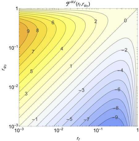
The vacuum polarisation tensor for the $ZV$ mixing, in contrast, is more involved due to the non-vector nature of the couplings on both sides of the loop. Its transverse and longitudinal components in the $q^{2}\to 0$ limit read

	$\displaystyle\Pi^{ZV}_{T}(q^{2}\to 0)$	$\displaystyle\sim$	$\displaystyle{gg_{D}\over 64\pi^{2}c_{w}}\bigg[3m_{f}^{2}\mathcal{F}_{m}^{ZV}(r_{f},r_{\psi_{D}})+q^{2}\bigg(\mathcal{F}_{qT1}^{ZV}(r_{f},r_{\psi_{D}})+Q_{f}s_{W}^{2}\mathcal{F}_{qT2}^{ZV}(r_{f},r_{\psi_{D}})\bigg)\bigg]\;,$		(41)
	$\displaystyle\Pi^{ZV}_{L}(q^{2}\to 0)$	$\displaystyle\sim$	$\displaystyle{gg_{D}\over 64\pi^{2}c_{w}}\bigg[3m_{f}^{2}\mathcal{F}_{m}^{ZV}(r_{f},r_{\psi_{D}})+q^{2}\mathcal{F}_{qL}^{ZV}(r_{f},r_{\psi_{D}})\bigg]\;,$		(42)

such that the total contribution is

\Pi^{ZV}(q^{2}\to 0)\sim{gg_{D}\over 64\pi^{2}c_{w}}\bigg[6m_{f}^{2}\mathcal{F}_{m}^{ZV}(r_{f},r_{\psi_{D}})+q^{2}\bigg(\mathcal{F}_{qT1+qL}^{ZV}(r_{f},r_{\psi_{D}})+Q_{f}s_{W}^{2}\mathcal{F}_{qT2}^{ZV}(r_{f},r_{\psi_{D}})\bigg)\bigg]\;,

(43)

where the functions $\mathcal{F}_{m,qT1+qL,qT2}^{ZV}(r_{f},r_{\psi_{D}})$ are provided in appendix B and their numerical values are shown in fig. 4.

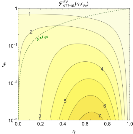
Besides the kinetic mixing, a mass mixing is thus induced between the SM $Z$ boson and $V^{\prime}$ . The coefficients of the $ZV$ kinetic and mass mixing read:

	$\displaystyle\epsilon_{ZV}$	$\displaystyle=$	$\displaystyle{gg_{D}\over 64\pi^{2}c_{w}}\bigg(\mathcal{F}_{qT1+qL}^{ZV}(r_{f},r_{\psi_{D}})+Q_{f}s_{W}^{2}\mathcal{F}_{qT2}^{ZV}(r_{f},r_{\psi_{D}})\bigg)\;,$		(44)
	$\displaystyle\Delta m^{2}_{ZV}$	$\displaystyle=$	$\displaystyle{3gg_{D}\over 32\pi^{2}c_{w}}m_{f}^{2}\mathcal{F}_{m}^{ZV}(r_{f},r_{\psi_{D}})\;.$		(45)

The adimensional function $F_{m}^{ZV}(r_{f},r_{\psi_{D}})$ appearing in the expression of the mass shift $\Delta m^{2}_{ZV}$ is small for $r_{\psi_{D}}\simeq 1$ (i.e., in the decoupling limit) and rapidly grows as $r_{\psi_{D}}$ decreases. The function $F_{qT1+qL}^{ZV}(r_{f},r_{\psi_{D}})$ has a similar behaviour but with a milder dependence on $r_{\psi_{D}}$ . The function $F_{qT2}^{ZV}(r_{f},r_{\psi_{D}})$ has a similar behaviour as $\mathcal{F}^{AV}(r_{f},r_{\psi_{D}})$ .

The mass matrix of the $(Z_{\mu}\;V^{\prime}_{\mu})$ system receives a shift proportional to the mass term in the vacuum polarisation tensor:

\tilde{M}^{2}_{ZV}=\left(\begin{array}[]{cc}{1\over 4}(g^{2}+g^{\prime 2})v^{2}&{1\over 2}\Delta m^{2}_{ZV}\\ {1\over 2}\Delta m^{2}_{ZV}&{1\over 4}g_{D}^{2}v_{D}^{2}\end{array}\right)=\left(\begin{array}[]{cc}\tilde{m}_{Z}^{2}&{1\over 2}m_{f}^{2}\epsilon^{m}_{ZV}\\ {1\over 2}m_{f}^{2}\epsilon^{m}_{ZV}&\tilde{m}_{V^{\prime}}^{2}\end{array}\right)\;,

(46)

where the adimensional parameter $\epsilon^{m}_{ZV}=\Delta m^{2}_{ZV}/m_{f}^{2}$ has been introduced, and where loop contributions to the diagonal terms have been neglected because of the non-zero tree-level values. This matrix is rotated by $V^{\rm KM}$ into

M^{2}_{ZV}=\left(V^{\rm KM}\right)^{T}\tilde{M}^{2}_{ZV}V^{\rm KM}={1\over 4}\left(\begin{array}[]{cc}(g^{2}+g^{\prime 2})v^{2}&-{(g^{2}+g^{\prime 2})v^{2}\epsilon_{ZV}-2m_{f}^{2}\epsilon^{m}_{ZV}\over\sqrt{1-\epsilon_{AV}^{2}-\epsilon_{ZV}^{2}}}\\ -{(g^{2}+g^{\prime 2})v^{2}\epsilon_{ZV}-2m_{f}^{2}\epsilon^{m}_{ZV}\over\sqrt{1-\epsilon_{AV}^{2}-\epsilon_{ZV}^{2}}}&{g_{D}^{2}v_{D}^{2}+(g^{2}+g^{\prime 2})v^{2}\epsilon_{ZV}^{2}-4m_{f}^{2}\epsilon_{ZV}\epsilon^{m}_{ZV}\over 1-\epsilon_{AV}^{2}-\epsilon_{ZV}^{2}}\end{array}\right)

(47)

and diagonalised through a rotation with angle

\tan 2\theta_{ZV}=\pm{2\left((g^{2}+g^{\prime 2})v^{2}\epsilon_{ZV}-2m_{f}^{2}\epsilon^{m}_{ZV}\right)\sqrt{1-\epsilon_{AV}^{2}-\epsilon_{ZV}^{2}}\over(1-\epsilon_{AV}^{2}-\epsilon_{ZV}^{2})(g^{2}+g^{\prime 2})v^{2}-g_{D}^{2}v_{D}^{2}+4\epsilon_{ZV}\epsilon^{m}_{ZV}m_{f}^{2}}\;,

(48)

which is positive for $m_{V^{\prime}}>m_{Z}$ and negative otherwise, and in the limit of small $\epsilon_{AV},\epsilon_{ZV}$ and $\epsilon^{m}_{ZV}$ becomes:

\tan 2\theta_{ZV}\simeq 2\theta_{ZV}\simeq\pm 2{2m_{f}^{2}\epsilon^{m}_{ZV}-(g^{2}+g^{\prime 2})v^{2}\epsilon_{ZV}\over g_{D}^{2}v_{D}^{2}-(g^{2}+g^{\prime 2})v^{2}}\;.

(49)

In the same limit the masses of the $Z$ and $V^{\prime}$ bosons read:

	$\displaystyle m_{Z}^{2}$	$\displaystyle\simeq$	$\displaystyle{1\over 4}(g^{2}+g^{\prime 2})v^{2}\left[1+\theta_{ZV}^{2}\left(1-{g_{D}^{2}v_{D}^{2}\over(g^{2}+g^{\prime 2})v^{2}}\right)\right]\;,$		(50)
	$\displaystyle m_{V^{\prime}}^{2}$	$\displaystyle\simeq$	$\displaystyle{1\over 4}g_{D}^{2}v_{D}^{2}\left[1+\epsilon_{AV}^{2}+(\theta_{ZV}-\epsilon_{ZV})^{2}\left(1-{(g^{2}+g^{\prime 2})v^{2}\over g_{D}^{2}v_{D}^{2}}\right)\right]$		(51)

The induced modification to the $Z$ boson mass (and an analogous modification to the $W$ boson mass induced by loops involving $F$ and a SM particle, potentially contributing to the $W$ mass anomaly observed by Aaltonen et al. 2022) are constrained by EW precision data and depend on specific realisations of the model. Another source of $V_{D}$ and $V^{\prime}$ mass split are the different fermionic loop corrections from $f,F$ and $\psi_{D}$ corresponding to the different ${\mathbb{Z}}_{2}$ parities of the ${SU(2)_{\rm D}}$ gauge bosons, as shown in fig. 2. A detailed discussion of the 1-loop calculations is provided in appendix A. The mass splitting $\Delta m_{V}=m_{V_{D}}-m_{V^{\prime}}$ can be written in a compact form in terms of the parameters

\epsilon_{1}=\frac{m_{F}^{2}-m_{\psi_{D}}^{2}}{m_{F}^{2}},\quad\epsilon_{2}=\frac{m_{f}^{2}}{m_{F}^{2}},\quad\epsilon_{3}=\frac{m_{V_{D}}^{2}}{m_{F}^{2}}\;.

(52)

In the approximation of $\epsilon_{1},\epsilon_{2},\epsilon_{3}\ll 1$ one has

\Delta m_{V}^{\prime}\equiv\Delta m_{V}\big|_{\epsilon,\epsilon_{2},\epsilon_{3}\ll 1}=\frac{1}{640\pi^{2}m_{V_{D}}}\epsilon_{1}^{2}g_{D}^{2}m_{F}^{2}\left[(20+3\epsilon_{3}-15\epsilon_{2}+20\epsilon_{2}\epsilon_{3})+10(3\epsilon_{2}-\epsilon_{3}-2\epsilon_{2}\epsilon_{3})\log\epsilon_{3}\right]+o(\epsilon_{1}^{2},\epsilon_{2},\epsilon_{3})\;.

(53)

For practical purposes, the expression for $\Delta m_{V}$ can be further simplified by neglecting $\epsilon_{2}$ and $\epsilon_{3}$ and keeping the leading term in $\epsilon_{1}$ , which leads to the following simple form:

\Delta m_{V}^{\prime\prime}\equiv\Delta m_{V}^{\prime}\big|_{\epsilon_{2},\epsilon_{3}=0}=\frac{g_{D}^{2}m_{F}^{2}}{32\pi^{2}m_{V_{D}}}\epsilon_{1}^{2}=\frac{g_{D}^{2}m_{F}^{2}}{32\pi^{2}m_{V_{D}}}\left(\frac{m_{F}^{2}-m_{\psi_{D}}^{2}}{m_{F}^{2}}\right)^{2}.

(54)

The radiative mass splitting between the $V_{D}$ and $V^{\prime}$ bosons plays a very important role in the determination of relic density and DM Indirect Detection (ID) rates. The range of validity of the approximations for $\Delta m_{V}$ presented above depends on the specific realisation of the FPVDM model and its parameter space. A detailed discussion of the respective numerical results for $\Delta m_{V}$ is given in section IV for a specific case study.

Finally, it is important to mention that the covariant derivative is modified by the kinetic mixing as follows:

D_{\mu}\simeq\partial_{\mu}-ieQA_{\mu}-i\left[{g\over c_{w}}(T_{3}-Qs_{W}^{2})-g_{D}T^{3}_{D}\theta_{ZV}\right]Z_{\mu}-i\left[g_{D}T^{3}_{D}-eQ\epsilon_{AV}+{g\over c_{w}}(T_{3}-Qs_{W}^{2})(\theta_{ZV}-\epsilon_{ZV})\right]V^{\prime}_{\mu}\;\quad,

(55)

where we have included only leading terms in $\theta_{ZV}$ and $\epsilon_{ZV}$ .

This modification has certain phenomenological consequences. Among the most relevant ones, the interaction of $V^{\prime}$ with all charged SM particles via the mixing parameter $\epsilon_{AV}$ allows the direct production of $V^{\prime}$ at the LHC via Drell-Yan topologies, and is therefore constrained by direct searches of heavy resonances. Also, the DM candidate $V_{D}$ can interact through EM multipoles with atomic matter, contributing to direct detection observables Hisano et al. 2020. In the case where only one VL representation is present, the constraints coming from these processes depend only on the fermion charge $Q$ and on the mass ratios $r_{f}$ and $r_{\psi_{D}}$ , but not on the specific flavour of the fermion.

II.3.3 Scalars

The scalar potential of eq. (13) is constructed starting from the 8 degrees of freedom of all the scalar fields of the theory: 4 for $\Phi_{H}$ and 4 for $\Phi_{D}$ . The theory contains 6 massive gauge bosons: $Z$ , $W^{\pm}$ , $V^{\prime}$ and $V_{D}$ (with two opposite D-isospin values). Therefore 6 Goldstone bosons are needed to give the corresponding longitudinal components. Thus, 2 degrees of freedom are left, which correspond to physical massive scalars: the SM Higgs boson, $h$ , and a further CP-even scalar, $H$ . Upon expressing the neutral scalars in the interaction eigenstates in terms of their components in the unitary gauge as

	$\displaystyle\phi^{0}$	$\displaystyle={1\over\sqrt{2}}(v+h_{1})\;,$		(56)
	$\displaystyle\varphi^{0}_{D-1/2}$	$\displaystyle={1\over\sqrt{2}}(v_{D}+\varphi_{1})\;,$		(57)

the Lagrangian terms for scalar masses can be written as:

{\mathcal{L}}_{m}^{\mathcal{S}}=-(h_{1}\;\varphi_{1})\left(\begin{array}[]{cc}\lambda v^{2}&{\lambda_{\Phi_{H}\Phi_{D}}\over 2}vv_{D}\\ {\lambda_{\Phi_{H}\Phi_{D}}\over 2}vv_{D}&\lambda_{D}v_{D}^{2}\end{array}\right)\left(\begin{array}[]{c}h_{1}\\ \varphi_{1}\end{array}\right)\;.

(58)

The mass eigenvalues are obtained by diagonalising the mass matrix via a rotation matrix $V_{S}=\left(\begin{array}[]{cc}\cos\theta_{S}&\sin\theta_{S}\\ -\sin\theta_{S}&\cos\theta_{S}\end{array}\right)$ and are

m_{h,H}^{2}=\lambda v^{2}+\lambda_{D}v_{D}^{2}\mp\sqrt{(\lambda v^{2}-\lambda_{D}v_{D}^{2})^{2}+\lambda_{\Phi_{H}\Phi_{D}}^{2}v^{2}v_{D}^{2}}

(59)

whilst the mixing angle is

\sin\theta_{S}=\sqrt{2{m_{H}^{2}v^{2}\lambda-m_{h}^{2}v_{D}^{2}\lambda_{D}\over m_{H}^{4}-m_{h}^{4}}}\;.

(60)

Even in the absence of explicit mixing induced by the quadratic term, i.e., even if $\lambda_{\Phi_{H}\Phi_{D}}=0$ , $h_{1}$ and $\varphi_{1}$ can mix at one-loop via the their interactions with fermions. The consequences of this mixing, which can also affect Higgs-related observables, go beyond the scopes of this analysis, and will be treated in a future work.

II.4 Flavour structure and Cabibbo-Kobayashi-Maskawa (CKM) matrix

The previous treatment assumed the presence of one VL ${SU(2)_{\rm D}}$ doublet interacting with one SM fermion, without specifying the flavour structure involved. If the full flavour structure of the SM is considered, different possibilities might arise. A VL fermion can interact with one or more SM flavours and there can be multiple VL fermions.

The most general Lagrangian, accounting for the above-mentioned possibilities, is

$\displaystyle{\mathcal{L}}_{m}$	$\displaystyle=$	$\displaystyle M_{U}^{I}\bar{U}_{I}U_{I}+M_{D}^{J}\bar{D}_{J}D_{J}+M_{E}^{K}\bar{E}_{K}E_{K}$	(61)
	$\displaystyle+$	$\displaystyle y_{u}^{i}\bar{Q}_{iL}^{\rm SM}\tilde{\Phi}_{H}u^{\rm SM}_{iR}+y_{d}^{i}\tilde{V}_{\rm CKM}^{ij}\bar{Q}^{\rm SM}_{iL}\Phi_{H}d^{\rm SM}_{jR}+y_{l}^{i}\bar{L}^{\rm SM}_{iL}\Phi_{H}l^{\rm SM}_{iR}+h.c.$
	$\displaystyle+$	$\displaystyle(y^{\prime}_{u})^{Ij}\bar{U}_{IL}\Phi_{D}u^{\rm SM}_{jR}+(y^{\prime}_{d})^{Jj}\bar{D}_{JL}\Phi_{D}d^{\rm SM}_{jR}+(y^{\prime}_{l})^{Kj}\bar{E}_{KL}\Phi_{D}l^{\rm SM}_{jR}+h.c.\;,$

where $\tilde{\Phi}_{H}=i\tau_{2}\Phi_{H}^{*}$ , $i,j=1,2,3$ are SM flavour indices and $I,J,K$ run over the flavours of the VL partners. The SM Yukawa couplings have been diagonalised exploiting the flavour symmetries and the SM CKM matrix (i.e., the CKM matrix if no VL states were introduced) and $\tilde{V}_{\rm CKM}$ has been introduced to parametrise the misalignment between the flavour and mass eigenstates in the down sector.

The most generic mass matrices read as follows:

\mathcal{M}_{U}=\left(\begin{array}[]{c|c}y_{u}^{i}{v\over\sqrt{2}}&0^{iI}\\ \hline\cr(y_{u}^{\prime})^{Ii}{v_{D}\over\sqrt{2}}&M_{U}^{I}\end{array}\right)\;,\quad\mathcal{M}_{D}=\left(\begin{array}[]{c|c}y_{d}^{i}\tilde{V}_{\rm CKM}^{ij}{v\over\sqrt{2}}&0^{iJ}\\ \hline\cr(y_{d}^{\prime})^{Ji}{v_{D}\over\sqrt{2}}&M_{D}^{J}\end{array}\right)\;,\quad\mathcal{M}_{E}=\left(\begin{array}[]{c|c}y_{l}^{i}{v\over\sqrt{2}}&0^{iK}\\ \hline\cr(y_{l}^{\prime})^{Ki}{v_{D}\over\sqrt{2}}&M_{E}^{K}\end{array}\right)\;.

(62)

The mass matrices can be diagonalised by two unitary matrices $V_{L}$ and $V_{R}$ , with dimension $3+\{I,J,K\}$ depending on the fermion type. If the same VL fermion interacts with multiple flavours of SM fermions, the most constraining effects are represented by modifications to SM observables, induced by Flavour Changing Neutral Currents (FCNCs) Cacciapaglia et al. 2012; Okada and Panizzi 2013. If for each SM fermion there is a VL partner, the matrix proportional to $y^{\prime}$ is diagonal as well and no mixing is induced between different SM and VL flavours, thus fermions from the dark sector only interact with the corresponding SM flavour. In the following we will limit the analysis to this simpler scenario.

An important property of this construction is that the CKM matrix of the SM receives contributions from new physics. In fact, the SM charged current is

	$\displaystyle J_{W^{+}}^{\mu}$	$\displaystyle=$	$\displaystyle{g\over\sqrt{2}}(\bar{u}^{\rm SM\;i}_{L}\;\bar{U}_{L}^{I})\gamma^{\mu}\left(\begin{array}[]{c\|c}1_{3\times 3}&0^{3J}\\ \hline\cr 0^{I3}&0^{IJ}\end{array}\right)\left(\begin{array}[]{c}d_{L}^{\rm SM\;i}\\ D^{J}_{L}\end{array}\right)$
		$\displaystyle=$	$\displaystyle{g\over\sqrt{2}}(\bar{u}_{L}^{i}\;\bar{u}_{L}^{\prime I})\gamma^{\mu}V_{uL}^{\dagger}\left(\begin{array}[]{c\|c}\tilde{V}_{\rm CKM}&0^{3J}\\ \hline\cr 0^{I3}&0^{IJ}\end{array}\right)V_{dL}\left(\begin{array}[]{c}d^{i}_{L}\\ d^{\prime J}_{L}\end{array}\right)\;,$

such that the entries of the measured CKM matrix are given by

V_{CKM}^{ij}=(V_{uL}^{\dagger})^{ik}\tilde{V}_{\rm CKM}^{kl}V_{dL}^{kj}\;.

(73)

II.5 FPVDM parameter space

The Lagrangian parameters of the model are the following:

•

gauge couplings: $g,g^{\prime},g_{D}$ ;
•

Scalar potential parameters: $\mu,\lambda,\mu_{D},\lambda_{D},\lambda_{\Phi_{H}\Phi_{D}}$ ;
•

Yukawa couplings and VL quark mass: $y,y^{\prime},m_{\psi_{D}}$ ;
•

$\tilde{V}_{\rm CKM}$ parameters.

Assuming that the new VL fermion interacts only with one SM flavour, these parameters can be traded for the masses of all the physical states, the weak coupling constant $g$ (or equivalently, the fine structure constant $\alpha_{\rm EM}$ ), the new gauge coupling $g_{D}$ , the mixing angle between the scalar fields $\theta_{S}$ and the measured CKM parameters. A complete set of parameters is therefore:

\displaystyle\{g,m_{W},m_{Z}\},~\{g_{D},m_{V_{D}}\},~\{m_{h},m_{H},\sin\theta_{S}\},~\{m_{f},m_{F},m_{\psi_{D}}\}~\text{and}~V_{\rm CKM}\;,

(74)

but, since ${g,m_{W},m_{Z}}$ , $m_{h}$ , $m_{f}$ and $V_{\rm CKM}$ are precisely measured SM parameters, we are left with the following six independent new physics parameters, namely:

\displaystyle g_{D},m_{V_{D}},m_{H},\sin\theta_{S},m_{F},m_{\psi_{D}}\;.

(75)

Approximating the CKM as a diagonal matrix for simplicity, the relations between the Lagrangian parameters connected to the new physics components and the input parameters take a very simple form:

$\displaystyle v$	$\displaystyle=$	$\displaystyle{2m_{W}\over g},\quad v_{D}={2m_{V_{D}}\over g_{D}}\;,$	(76)
$\displaystyle\lambda$	$\displaystyle=$	$\displaystyle{g^{2}\over 8m_{W}^{2}}(m_{h}^{2}\cos^{2}\theta_{S}+m_{H}^{2}\sin^{2}\theta_{S})\;,$	(77)
$\displaystyle\lambda_{D}$	$\displaystyle=$	$\displaystyle{g_{D}^{2}\over 8m_{V_{D}}^{2}}(m_{h}^{2}\sin^{2}\theta_{S}+m_{H}^{2}\cos^{2}\theta_{S})\;,$	(78)
$\displaystyle\lambda_{\Phi_{H}\Phi_{D}}$	$\displaystyle=$	$\displaystyle{g\;g_{D}\over 8m_{W}m_{V_{D}}}(m_{H}^{2}-m_{h}^{2})\sin 2\theta_{S}\;,$	(79)
$\displaystyle\mu^{2}$	$\displaystyle=$	$\displaystyle{1\over 2}\left(m_{h}^{2}\cos^{2}\theta_{S}+m_{H}^{2}\sin^{2}\theta_{S}+{1\over 2}{g\over g_{D}}{m_{V_{D}}\over m_{W}}(m_{H}^{2}-m_{h}^{2})\sin 2\theta_{S}\right)\;,$	(80)
$\displaystyle\mu_{D}^{2}$	$\displaystyle=$	$\displaystyle{1\over 2}\left(m_{h}^{2}\sin^{2}\theta_{S}+m_{H}^{2}\cos^{2}\theta_{S}+{1\over 2}{g_{D}\over g}{m_{W}\over m_{V_{D}}}(m_{H}^{2}-m_{h}^{2})\sin 2\theta_{S}\right)\;,$	(81)
$\displaystyle y$	$\displaystyle=$	$\displaystyle{g\;m_{f}\;m_{F}\over\sqrt{2}m_{\psi_{D}}m_{W}}\;,$	(82)
$\displaystyle y^{\prime}$	$\displaystyle=$	$\displaystyle{g_{D}\sqrt{(m_{F}^{2}-m_{\psi_{D}}^{2})(m_{\psi_{D}}^{2}-m_{f}^{2})}\over\sqrt{2}m_{\psi_{D}}m_{V_{D}}}\;.$	(83)

The minimisation conditions of the scalar potential in eq. (II.2) are automatically satisfied. If $\lambda_{\Phi_{H}\Phi_{D}}<0$ , which corresponds to $m_{h}>m_{H}$ , the condition $\lambda_{\Phi_{H}\Phi_{D}}^{2}<4\lambda\lambda_{D}$ translates into ${1\over 16}{g^{2}g_{D}^{2}\over m_{W}^{2}m_{V_{D}}^{2}}m_{h}^{2}m_{H}^{2}>0$ , which is always true, whilst, if $\lambda_{\Phi_{H}\Phi_{D}}>0$ , the conditions $2\lambda\mu_{D}^{2}>\lambda_{\Phi_{H}\Phi_{D}}\mu^{2}$ and $2\lambda_{D}\mu^{2}>\lambda_{\Phi_{H}\Phi_{D}}\mu_{D}^{2}$ translate into ${1\over 8}{g^{2}\over m_{W}^{2}}m_{h}^{2}m_{H}^{2}>0$ and ${1\over 8}{g_{D}^{2}\over m_{V_{D}}^{2}}m_{h}^{2}m_{H}^{2}>0$ , respectively, again automatically satisfied.

For a perturbative analysis of the parameter space we need to identify the regions where coupling parameters do not become too large, in order to make sure that all predictions on the model are reliable. A complete loop description of all the sectors of the model is beyond the scope of this analysis and therefore we assume that perturbativity is achieved by the requirement for all couplings of the FPVDM model to be (optimistically) below $4\pi$ . For example, the requirement $\lambda<4\pi$ defines the maximal value of $m_{H}$ for a given value of the scalar mixing angle, $\theta_{S}$ , as shown by the blue contour in the left panel of fig. 5. The same figure presents contours for the $g_{D}/m_{V_{D}}$ ratio in the $\{m_{H},\theta_{S}\}$ plane corresponding to $\lambda_{D}=4\pi$ , which indicates the perturbativity limit on the respective parameters.

The perturbative constraints on the Yukawa couplings $y$ and $y^{\prime}$ imply that the ratio between the masses of the new fermions $F$ and $\psi_{D}$ cannot be too large. The condition for $y$ reads as ${m_{F}\over m_{\psi_{D}}}<4\pi{\sqrt{2}m_{W}\over gm_{f}}$ . At the same time, the $y^{\prime}<4\pi$ condition is defined also by the $g_{D}/m_{V_{D}}$ ratio, as one can see from eq. (83). Both constraints from $y$ and $y^{\prime}$ perturbativity requirements are presented in the right panel of fig. 5 in the $(m_{\psi_{D}},{m_{F}\over m_{\psi_{D}}})$ plane. In our analysis of the parameter space we indicate the respective regions where perturbativity constraints are violated.

III On the origin of the global $U(1)$ symmetry

One of the main open questions of the construction presented in this analysis is the origin of the global $U(1)$ symmetry (with its ${\mathbb{Z}}_{2}$ parity subset) which has to be imposed to avoid the contemporary presence of two Yukawa interactions involving $\Phi_{D}$ and $\Phi_{D}^{*}$ which would explicitly break ${SU(2)_{\rm D}}$ , and therefore spoil the stability of the DM candidate. A theoretical origin of the symmetry would provide a robust ground for the consistency of the model. In this section we explore two options for explaining such origin. The first involves promoting the global $U(1)$ to a local gauge symmetry, $U(1)_{\rm D}$ , in the dark sector, which would generate a mirror version of the SM EW sector in the dark sector, the two of which can be connected by the mixed $(\Phi^{\dagger}\Phi)(\Phi_{D}^{\dagger}\Phi_{D})$ quartic term in the full potential and by the gauge kinetic mixing between $U(1)_{Y}$ and $U(1)_{D}$ . In this scenario the $U(1)_{\rm D}$ local symmetry would be associated to a conserved dark-charge completely analogous to the EM charge of QED, thus giving literal meaning to the notation $V^{0}_{D0}$ and $V^{0}_{D\pm}$ for the ${SU(2)_{\rm D}}$ gauge bosons in the dark sector.

The second involves the existence of a strongly-coupled sector whose condensates form the particle in the low energy regime, in particular, a residual parity for the composite sector is present due to the specific vacuum alignment present in this kind of models (which would typically also imply an extended Higgs sector). A detailed discussion is given in Ma and Cacciapaglia 2016 and further used in Wu et al. 2017 for the case of a scalar DM candidate.

III.1 A dark electroweak sector

In this scenario the SM is augmented with a dark sector constructed starting from a dark gauge group $\mathcal{G}_{D}$ with same structure as the EW gauge group of the SM. The gauge group is spontaneously broken as:

\mathcal{G}=\mathcal{G}_{\rm SM}\times\mathcal{G}_{D}=SU(2)_{L}\times U(1)_{Y}\times{SU(2)_{\rm D}}\times{U(1)_{\rm YD}}\longrightarrow U(1)_{\rm EM}\times{U(1)_{\rm D}}\;.

(84)

The gauge boson associated to ${U(1)_{\rm YD}}$ is labelled as $B^{0}_{D0\mu}$ . The full covariant derivative is

D_{\mu}=\partial_{\mu}-\left(i{g\over\sqrt{2}}W^{\pm}_{\mu}T^{\pm}+igW^{3}_{\mu}T_{3}+ig^{\prime}YB_{\mu}\right)-\left(i{g_{D}\over\sqrt{2}}V^{0}_{D\pm\mu}T^{\pm}_{D}+ig_{D}V^{0}_{D0\mu}T_{3D}+ig^{\prime}_{D}Y_{D}B^{0}_{D0\mu}\right)\;,

(85)

where $g$ and $g^{\prime}$ are, respectively, the weak and hypercharge coupling constants, $g_{D}$ and $g_{D}^{\prime}$ are the ${SU(2)_{\rm D}}$ and ${U(1)_{\rm YD}}$ coupling constants, $T_{3}$ and $Y$ are the weak-isospin and weak-hypercharge, $T_{3D}$ and $Y_{D}$ are the dark-isospin associated with ${SU(2)_{\rm D}}$ and the dark-hypercharge associated with ${U(1)_{\rm YD}}$ and where the indices of the $T_{D}$ matrices act only on the ${SU(2)_{\rm D}}$ elements and are diagonal with respect $SU(2)_{L}$ while the indices of the $T$ matrices act only on the $SU(2)$ elements and are diagonal with respect to ${SU(2)_{\rm D}}$ .

The unbroken $U(1)_{\rm D}$ continuous symmetry is associated to a conserved charge, labelled D-charge, defined as:

Q_{D}=T_{3D}+Y_{D}\;.

(86)

Notice that the D-charge is not associated with the electric charge: electrically neutral particles can be D-charged and vice versa. The only assumption to be made in this scenario is that all the SM states are neutral under the conserved D-charge $Q_{D}$ . This however does not necessarily imply that all the states of new physics are charged under ${U(1)_{\rm D}}$ or that they must be neutral under the conserved SM charges.

The fields responsible for the breaking of the gauge symmetry are the two scalar doublets $\Phi_{H}$ and $\Phi_{D}$ described in section II. Since $\Phi_{H}$ is singlet with respect to the dark gauge group and $\Phi_{D}$ is singlet with respect to the EW gauge group, given the absence of gauge kinetic mixing terms, no mixing is induced between the fully neutral gauge bosons $W_{\mu}^{3}$ , $B_{\mu}$ , $V^{0}_{D0\mu}$ and $B^{0}_{D0\mu}$ . In complete analogy with the SM, by counting the number of bosonic degrees of freedom, one massless gauge boson is predicted in the dark gauge sector and the other dark gauge bosons receive different masses. We can thus define the mass eigenstates $\gamma_{D}$ , $Z^{0}_{D}$ and $W^{0}_{D\pm}$ with values

$\displaystyle M_{\gamma_{D}}$	$\displaystyle=$	$\displaystyle 0\;,$	(87)
$\displaystyle M_{Z^{0}_{D}}$	$\displaystyle=$	$\displaystyle{1\over 2}\sqrt{g_{D}^{2}+g^{\prime 2}_{D}}~v_{D}\;,$	(88)
$\displaystyle M_{W^{0}_{D\pm}}$	$\displaystyle=$	$\displaystyle{g_{D}\over 2}v_{D}\;,$	(89)

such that the masses of the DM vector $V^{0}_{D\pm}$ and of the D-charge-neutral gauge boson $V^{0}_{D0}$ receive a splitting proportional to ${1\over 2}g^{\prime}_{D}v_{D}$ . The particle content of the model is summarised in Table 2. One should note that the presence of the massless dark radiation from the unbroken $U(1)$ is not necessarily a problem as soon as it does not contribute too much to relativistic degrees of freedom at BBN and allows the formation of structures as small scales. As shown in Ackerman et al. 2009, for example, it can be achieved when at the DM decouples from the dark radiation at high redshifts.

Scalar fields
	EW		Dark		Unbroken
	$SU(2)_{L}$	$U(1)_{Y}$	${SU(2)_{\rm D}}$	$U(1)_{\rm YD}$	$U(1)_{\rm EM}$	$U(1)_{\rm D}$
$\Phi_{H}=\left(\begin{array}[]{c}\phi^{+}\\ \phi^{0}\end{array}\right)$	$\mathbf{2}$	$1/2$	$\mathbf{1}$	$0$	1	0
	$\mathbf{2}$	$1/2$	$\mathbf{1}$	$0$	0	0
$\Phi_{D}=\left(\begin{array}[]{c}\varphi^{0}_{D+{1\over 2}}\\ \varphi^{0}_{D-{1\over 2}}\end{array}\right)$	$\mathbf{1}$	$0$	$\mathbf{2}$	$1/2$	$\begin{array}[]{c}0\\ 0\end{array}$	$\begin{array}[]{c}1\\ 0\end{array}$
Fermion fields
$f_{L}^{\rm SM}=\left(\begin{array}[]{c}f_{u,\nu}^{\rm SM}\\ f_{d,\ell}^{\rm SM}\end{array}\right)_{\!\!\!L}$	$\mathbf{2}$	$1/6,-1/2$	$\mathbf{1}$	0	$T_{3f}+Y_{f}$	0
$u_{R}^{\rm SM},\nu_{R}^{\rm SM}$	$\mathbf{1}$	$2/3,0$	$\mathbf{1}$	0	$T_{3f}+Y_{f}$	0
$d_{R}^{\rm SM},\ell_{R}^{\rm SM}$	$\mathbf{1}$	$-1/3,-1$	$\mathbf{1}$	0	$T_{3f}+Y_{f}$	0
$\Psi=\left(\begin{array}[]{c}\psi^{D}\\ \psi\end{array}\right)$	$\mathbf{1}$	$Q_{\Psi}$	$\mathbf{2}$	$1/2$	$Q_{\Psi}$	$1$
	$\mathbf{1}$	$Q_{\Psi}$	$\mathbf{2}$	$1/2$	$Q_{\Psi}$	$0$
Vector fields
$W_{\mu}=\left(\begin{array}[]{c}W^{+}_{\mu}\\ W^{3}_{\mu}\\ W^{-}_{\mu}\end{array}\right)$	$\mathbf{3}$	$0$	$\mathbf{1}$	$0$	$\begin{array}[]{c}1\\ 0\\ -1\end{array}$	$\begin{array}[]{c}0\\ 0\\ 0\end{array}$
$B_{\mu}$	$\mathbf{1}$	0	$\mathbf{1}$	$0$	0	0
$V_{D\mu}=\left(\begin{array}[]{c}V^{0}_{D+\mu}\\ V^{0}_{D0\mu}\\ V^{0}_{D-\mu}\end{array}\right)$	$\mathbf{1}$	$0$	$\mathbf{3}$	$0$	$\begin{array}[]{c}0\\ 0\\ 0\end{array}$	$\begin{array}[]{c}1\\ 0\\ -1\end{array}$
$B^{0}_{D0\mu}$	$\mathbf{1}$	0	$\mathbf{1}$	$0$	0	0

Table 2: The quantum numbers under the EW and dark gauge group

{SU(2)_{\rm D}}\times U(1)_{\rm D}

of the particles of the model. The charges of the unbroken groups

U(1)_{\rm EM}

and

U(1)_{\rm D}

are also provided.

The presence of two $U(1)$ gauge groups, however, allows for the existence of a renormalisable and gauge-invariant kinetic mixing term already in the unbroken EW and dark symmetry phases, such that the Lagrangian of the $U(1)_{Y}\times U(1)_{\rm YD}$ sector is

-{\mathcal{L}}_{\rm KM}={1\over 4}B_{\mu\nu}B^{\mu\nu}+{1\over 4}B_{D\mu\nu}B_{D}^{\mu\nu}+{\varepsilon\over 2}B_{\mu\nu}B_{D}^{\mu\nu}\;,

(90)

where $B_{D\mu\nu}$ is the field tensor of $U(1)_{\rm YD}$ and $\varepsilon$ is the kinetic mixing parameter. The diagonalisation of the kinetic terms can be obtained through the rotation Feldman et al. 2007:

\left(\begin{array}[]{c}B^{\mu}\\ B^{0\mu}_{D0}\end{array}\right)=\left(\begin{array}[]{cc}{1\over\sqrt{1-\varepsilon^{2}}}&0\\ -{\varepsilon^{2}\over\sqrt{1-\varepsilon^{2}}}&1\end{array}\right)\left(\begin{array}[]{cc}\cos\theta_{k}&-\sin\theta_{k}\\ \sin\theta_{k}&\cos\theta_{k}\end{array}\right)\left(\begin{array}[]{c}B_{1}^{\mu}\\ B_{2}^{\mu}\end{array}\right)

(91)

The kinetic-mixing term induces a modification in the mass mixing matrix of the fully neutral gauge bosons. Upon diagonalisation, two massless eigenstates are obtained, corresponding to the SM photon and to a massless dark photon, and two massive eigenstates, corresponding to the $Z$ boson and to a massive $Z^{\prime}$ boson. The full expressions of the mass mixing matrix and of the mass eigenstates can be found in appendix C. Expanding the mass eigenstates of $Z$ and $Z^{\prime}$ for small $\varepsilon$ , the lowest order terms assume a simple form:

	$\displaystyle M_{Z}^{2}$	$\displaystyle=$	$\displaystyle{v^{2}\over 4}\left[g^{2}+g^{\prime 2}\left(1+{(g^{2}+g^{\prime 2})v^{2}-g_{D}^{2}v_{D}^{2}\over(g^{2}+g^{\prime 2})v^{2}-(g_{D}^{2}+g_{D}^{\prime 2})v_{D}^{2}}\varepsilon^{2}\right)\right]+\mathcal{O}(\varepsilon^{4})\;,$		(92)
	$\displaystyle M_{Z^{\prime}}^{2}$	$\displaystyle=$	$\displaystyle{v_{D}^{2}\over 4}\left[g_{D}^{2}+g_{D}^{\prime 2}\left(1+{g^{2}v^{2}-(g_{D}^{2}+g_{D}^{\prime 2})v_{D}^{2}\over(g^{2}+g^{\prime 2})v^{2}-(g_{D}^{2}+g_{D}^{\prime 2})v_{D}^{2}}\varepsilon^{2}\right)\right]+\mathcal{O}(\varepsilon^{4})\;,$		(93)

which in the $\varepsilon\to 0$ limit (no kinetic mixing) reduce to the SM value and eq.(88), respectively. Of course, analogously to the FPVDM model with the global $U(1)$ symmetry, after spontaneous breaking of EW and dark symmetries, kinetic and mass mixing terms arise at loop level as illustrated in section II.3.2, involving the four electrically and D-charge neutral gauge bosons. The implications of this scenario and the derivation of its experimental bounds are beyond the scope of this analysis and are reserved for future developments.

III.2 A composite origin

In the case of composite models the discrete symmetries allowing the stability of the DM particle depend on the model building details of the composite sector. However, this does not mean that the DM candidate and the corresponding discrete symmetries are an arbitrary choice. The composite effective chiral Lagrangian is invariant under a parity changing the signs of all the pseudo Nambu-Goldstone Bosons (pNGBs), as they appear in bilinear terms in the Lagrangian. Furthermore, these models contain by construction explicit symmetry breaking terms, so more scrutiny is needed to understand if a pNGB can be stable due to a residual parity and therefore be used as a particle describing DM. The origin of the non-invariance with respect to parity (and also charge conjugation) is due to the choice of the vacuum while the strong techni-sector at the origin of these models is instead parity invariant as it is VL with respect to the composite gauge dynamics and the SM gauge group. Once possible parities acting on the pNGBs are identified, these models require a careful check of their invariance, including the Wess-Zumino-Witten terms. In explicit realisations studied in the literature, e.g., in Ma and Cacciapaglia 2016; Wu et al. 2017, a stable pNGB multiplet allowing the description of DM can indeed be found.

IV A case study: top portal with no mixing between $h$ and $H$

This section is dedicated to a specific realisation of the model. It is assumed that only one VL partner exists, and interacts exclusively with the SM top quark. Moreover it is further assumed that the Higgs bosons $h$ and $H$ do not mix, i.e., $\theta_{S}=0$ . These choices significantly simplify the expressions of the Lagrangian parameters, which read:

$\displaystyle v$	$\displaystyle=$	$\displaystyle{2m_{W}\over g},~\mu^{2}={m_{h}^{2}\over 2},~\lambda={g^{2}m_{h}^{2}\over 8m_{W}^{2}},$	(94)
$\displaystyle v_{D}$	$\displaystyle=$	$\displaystyle{2m_{V_{D}}\over g_{D}},~\mu_{D}^{2}={m_{H}^{2}\over 2},~\lambda_{D}={g_{D}^{2}m_{H}^{2}\over 8m_{V_{D}}^{2}},~\lambda_{\Phi_{H}\Phi_{D}}=0,$	(95)
$\displaystyle y_{t}$	$\displaystyle=$	$\displaystyle{g\;m_{t}\;m_{T}\over\sqrt{2}m_{t_{D}}m_{W}}=y_{t}^{\rm SM}{m_{T}\over m_{t_{D}}},\quad y_{t}^{\prime}={g_{D}\sqrt{(m_{T}^{2}-m_{t_{D}}^{2})(m_{t_{D}}^{2}-m_{t}^{2})}\over\sqrt{2}m_{t_{D}}m_{V_{D}}}\;,$	(96)

where the ${\mathbb{Z}}_{2}$ -even(-odd) partner of the top quark has been labelled $T$ ( $t_{D}$ ), the SM Higgs sector is left unaffected by the new scalar, and $\Phi_{D}$ has a potential completely analogous to the Higgs potential. The hierarchy between the masses in the fermion sector is the same as that discussed in section II.3.1, i.e., $m_{t}<m_{t_{D}}\leq m_{T}$ , but $H$ can have any mass allowed by experimental bounds, including, in principle, being lighter than the SM Higgs boson.

The new physics parameter space for this model is five-dimensional:

g_{D},m_{V_{D}},m_{H},m_{T},m_{t_{D}}\;.

(97)

In the following, we will denote this scenario as TPVDM – a specific case of top portal in the FPVDM framework. We chose this realisation as a case study since, on the one hand, it is minimal whilst, on the other hand, it allows us to explore a scenario where a non-Abelian dark sector is not connected to the SM via a Higgs portal at tree level. Furthermore, connecting the dark sector only with the SM top quark allows for an exploration of several interesting collider physics signatures, whilst reducing the impact of constraints from direct detection.

Many other realisations are also very attractive. For example, the dark sector could be connected to SM leptons. The collider constraints on new VL leptons would then be milder, making the scenarios potentially less restricted, but the impact on the cosmological observables would not qualitatively change.²² 2 This is true except when the mass difference between DM and VL fermion mediator is small. In that case DM co-annihilation will be less intense in comparison with strong co-annihilation with the $t_{D}$ quark. These kind of realisations are potentially interesting for a study of anomalies in the lepton sector (for example in connection with the muon anomalous magnetic moment) and will be developed in future studies.

As anticipated in section II.3.2, the mass splitting between $m_{V_{D}}$ and $m_{V^{\prime}}$ , $\Delta m_{V}=m_{V_{D}}-m_{V^{\prime}}$ , plays an important role for DM phenomenology. First of all, we have found that $\Delta m_{V}>0$ in the whole parameter space of the model, with the approximate expressions for $\Delta m_{V}$ given by eqs. 53 and 54. Since $m_{V_{D}}>m_{V^{\prime}}$ , the $V_{D}V_{D}^{*}\to V^{\prime}V^{\prime}$ process for DM annihilation will always take place for any point in the parameter space to contribute crucially to the list of processes affecting the relic density and to extend the viable parameter space compatible with constraints imposed by the relic density. The $V_{D}V_{D}^{*}\to V^{\prime}V^{\prime}$ process also contributes to the DM indirect detection signals.

Numerically, the value of $\Delta m_{V}$ varies over a very wide range, since it scales as $g_{D}^{2}$ and it is proportional to $m_{T}^{2}-m_{t_{D}}^{2}$ . One should also note that $\Delta m_{V}$ does not depend on $m_{H}$ . In fig. 6 (left) we present the iso-contours for $\Delta m_{V}$ in the $\{m_{t_{D}},m_{V_{D}}\}$ plane for $g_{D}=0.1$ and $m_{T}=1600$ GeV, whilst in fig. 6 (right) we show how $\Delta m_{V}$ evolves as function of $m_{V_{D}}$ for the specific value of $m_{t_{D}}=1590$ GeV, all other parameters being the same. The value of $m_{T}$ is chosen to be safely above the current upper limit on VL top partners at the LHC Aaboud et al. 2018. For our particular choice of $g_{D}$ and $m_{T}$ , $\Delta m_{V}$ can be as large as 1 GeV, while its minimal value reaches zero for a vanishing value of $m_{T}-m_{t_{D}}$ . In both frames we present a comparison of the exact one-loop result for $\Delta m_{V}$ and its approximations given by eqs. 53 and 54. It is possible to see from fig. 6 (right) that the approximate formulae are very accurate for a small $m_{T}-m_{t_{D}}$ splitting, but break down for $m_{V_{D}}$ close to the $m_{t}+m_{\psi_{D}}$ threshold, where the one-loop corrections are highly non-linear in the expansion parameters used in approximate expressions for $\Delta m_{V}$ . Moreover, for small values of $m_{V_{D}}$ , the one-loop mass corrections can be large, making the evaluation of $\Delta m_{V}$ perturbatively unstable. Therefore, we indicate by the hatched area the region where one-loop corrections to the masses of $V_{D}$ and/or $V^{\prime}$ become larger than 50% of the corresponding bare masses.

The lifetime of $V^{\prime}$ does not directly depend on $\Delta m_{V}$ . However, the ${\mathbb{Z}}_{2}$ -even ${SU(2)_{\rm D}}$ gauge boson can also be long lived, if the DM is light enough. The only tree-level interaction of $V^{\prime}$ with SM particles is with top quarks, due to its mixing with $T$ . If the mass of $V^{\prime}$ drops below the $t\bar{t}$ threshold, it can only decay directly to a three-body or four-body final state with $W$ bosons and $b$ quarks via the off-shell top quarks, or decay to a $b\bar{b}$ final state at one-loop, see the Feynman diagrams in fig. 7 (left). The latter, although only present at the one-loop level, becomes dominant due to the reduced phase space for the four-body final state. This is shown in fig. 7 (centre and right). These loop-induced diagrams prevent $V^{\prime}$ from having a sufficiently long lifetime to spoil Big Bang Nucleo-synthesis (BBN). However, when the $g_{D}$ coupling is small, the $t_{D}$ mass approaches the decoupling limit ( $m_{t_{D}}=m_{T}$ ) and the DM is light, $V^{\prime}$ becomes long lived at colliders. Therefore, it could provide a signal for searches of long-lived neutral bosons decaying into $b\bar{b}$ pairs.

Figure 7: Left: Tree-level and one-loop diagrams for

V^{\prime}

decay. Center and right: decay width and lifetime of

V^{\prime}

at tree and one-loop level for

g_{D}=0.05

m_{T}=1600{\rm\ GeV}

and different values of

m_{t_{D}}

As mentioned in section II.3.3, even if TPVDM scenario does not contain a tree-level mixing, a loop-induced mixing between $h$ and $H$ still occurs, via SM top and the ${\mathbb{Z}}_{2}$ -even top ( $T$ ) loops. This contribution is eventually suppressed. A scenario with tree-level scalar mixing is more constrained and can exhibit the following signatures: 1) the heavy scalar $H$ can decay also to any final state accessible to the Higgs boson, and therefore the model predicts further signatures at collider; 2) if the mass of the DM is small enough, the Higgs boson will decay into the DM itself or the ${\mathbb{Z}}_{2}$ -even gauge boson $V^{\prime}$ , affecting its width and branching ratios. From the cosmological point of view, additional interactions from the tree-level scalar mixing will affect the relic density, and direct and indirect detection observables.

Since there is no $h$ - $H$ mixing in TPVDM scenario, DM scattering off the nuclei is induced only at loop-level. The Feynman diagrams for DM-gluon interactions with quark box and triangle topologies are shown in fig. 8(a) and (b), while the DM-quark diagrams generated by the loop-induced $V^{\prime}-\gamma/Z$ kinetic mixing and triangle diagrams are shown in fig. 8(c) and (d), respectively. The detailed evaluation of the triangle loop of fermions connected to gauge boson propagators is given in appendix D. As it will become clear in section IV.3, the KM and triangle contributions play a crucial role in constraining the parameter space of the model through Direct Detection (DD) limits on DM.

In the following sections, this model is tested against multiple observables from cosmology, direct DM detection experiments and LHC searches. For this analysis we implemented the Lagrangian of the model in the LanHEP Semenov 2009 and FeynRules Alloul et al. 2014 packages whilst model files have been generated in CalcHEP Belyaev et al. 2013, FeynArts Hahn 2001 and UFO Degrande et al. 2012 formats.³³ 3 The model implementations are available in the HEPMDB Bondarenko et al. 2012 repository in CalcHEP (https://hepmdb.soton.ac.uk/hepmdb:0322.0335) and UFO (https://hepmdb.soton.ac.uk/hepmdb:0322.0336) formats. We used micrOMEGAs v5.2.7 Belanger et al. 2021 for calculating DM observables and for setting the corresponding limits (see section IV.1) as well as for the evaluation of some LHC processes. The model implementation in UFO format has been used in MG5_aMC Alwall et al. 2014 for the determination of the complete set of LHC constraints (see section IV.2). The FeynArts model files from LanHEP were used to generated one-loop corrections to masses of $SU(2)_{\rm D}$ gauge bosons by FeynCalc Shtabovenko et al. 2020, FeynHelpers Shtabovenko 2017 and Package-X Patel 2017. A simplified version of the model has been implemented to calculate cross-sections at one-loop level in MG5_aMC and FormCalc9.8 Hahn et al. 2016.

IV.1 Constraints from DM relic density

There are many non-collider experiments dedicated to searching for signals of DM, both in space and on Earth which play a very important role in limiting the DM parameter space and in the identification of viable DM models. These experiments are devoted to the precise determination of the DM relic density as well as to DD and ID of DM. In particular, the PLANCK experiment has measured the relic density with a precision better than 1% Aghanim et al. 2020:

\Omega^{\text{Planck}}_{\text{DM}}h^{2}=0.12\pm 0.0012\,.

(98)

In our analysis, we will select points that satisfy this constraint, bearing in mind that points which predict a relic density below the PLANCK constraint could still be allowed if new sources of DM exist besides $V_{D}$ .

For DM DD we use the limits from XENON1T Aprile et al. 2018. The XENON1T experiment provides the most stringent upper limit (compared to LUX (2017) and Panda-X (2017), see fig. 5 in the reference Aprile et al. 2018). XENON1T provides the limit on DM-nucleon’s cross-section vs DM mass at $90\%$ C.L. together with the detector’s efficiency as a function of nuclear recoil energy. We have evaluated the DM-nucleon scattering cross section and converted it into the number of events by taking in account the efficiency of the XENON1T detector. This allowed us to find the corresponding p-value for the signal. The calculation was performed using a modified version of micrOMEGAs package which allowed us to correctly evaluate DM DD rates from the loop-induced $\gamma(Z)$ - $V_{D}$ - $V_{D}$ interactions. We have scaled the number of registered events if the corresponding relic density is less than the measured value as follows:

\displaystyle\hat{N}_{\text{event}}

\displaystyle=

\displaystyle\begin{cases}\left(\frac{\Omega_{\text{DM}}}{\Omega^{\text{Planck}}_{\text{DM}}}\right)N_{\text{event}},&\text{if}\ \Omega_{\text{DM}}h^{2}<0.12\\ N_{\text{event}},&\text{otherwise}\end{cases}\;,

(99)

and have defined the $p$ -value, $hat{p}$ , as

\displaystyle\hat{p}

\displaystyle=

\displaystyle\exp(-\hat{N}_{\text{event}})\;.

(100)

The exclusion of parameter space is imposed on the points where $\hat{p}<0.1$ , which corresponds to the exclusion limit at $90\%$ C.L.

ID DM searches are being performed by many experiments, including Fermi-LAT Ackermann et al. 2017, IceCube Aartsen et al. 2017, ANTARES Albert et al. 2020, etc. However, these experiments rely on the DM local density and velocity distribution as well as the propagation of the particles in the galactic plane. Therefore, the respective predictions are affected by various uncertainties of an astronomical nature. To be independent of these uncertainties, in this study we use the Cosmic Microwave Background (CMB) limit on DM ID based on PLANCK data. We consider the product of the DM-self annihilation or the DM decay into SM particles. By studying the effect of energy injection from DM annihilation products (electrons, positrons, gamma-ray, neutrinos and anti-protons) on the galactic medium which is sensitive to the CMB anisotropies, the upper limit on the energy injection measured by PLANCK is:

P_{\text{ann}}<3.2\times 10^{-28}\,\,\frac{\rm{cm^{3}}}{\rm{s\,GeV}}\quad\text{at 95\% C.L.,}

(101)

with

P_{\text{ann}}=\sum_{j}\frac{f^{\text{eff}}_{j}\braket{\sigma v}_{j}}{M_{\text{DM}}}\left(\frac{\Omega_{\text{DM}}}{\Omega^{\text{Planck}}_{\text{DM}}}\right)^{2},

(102)

where $\braket{\sigma v}_{j}$ is the thermally averaged partial annihilation cross-section for the $j$ channel whilst $f_{j}^{\text{eff}}$ is the energy fraction of DM annihilation transferring to the plasma for the $j$ th channel. To construct the quantity $P_{\text{ann}}$ , we use micrOMEGAs to calculate $\braket{\sigma v}_{j}$ for all possible channels and neglect those that contribute to the total annihilation cross-section less than $0.1\%$ . The effective fraction of energy $f^{\text{eff}}_{j}$ was thoroughly studied and provided for almost all DM annihilation processes into two SM particles in the final state in Slatyer 2016; Leane et al. 2018. For non-SM particles in the final state of $2\to 2$ processes, for example $V_{D},V_{D}\to V^{\prime},V^{\prime}/V^{\prime},H/H,H$ , we make the approximation $f^{\text{eff}}_{\text{non-SM}}\sim f^{\text{eff}}_{q\bar{q}}$ . This approximation is reasonable because each $V_{D}/H$ eventually decays into 3 pairs of quarks anti-quarks and the energy fractions stored in each quark anti-quark pair ( $u,d,s,c,b,t$ ) are not significantly different. The annihilation cross-section in eq. (102) is rescaled by $(\Omega_{\text{DM}}/\Omega^{\text{Planck}}_{\text{DM}})^{2}$ due to the two DM particles in the initial state.

Finally, we have checked that the model does not spoil the predictions from BBN. When the lifetime of $V^{\prime}$ is too long, such that it decays during or after BBN, it would spoile the observed neutron to proton density ratio. For $m_{V^{\prime}}\lesssim 2m_{W}$ , the dominant decay to $b\bar{b}$ via the loop-induced process discussed above makes $V^{\prime}$ lifetime much shorter than the value excluded by BBN. So, in this respect, BBN does not exclude any region of the parameter space of our model that is allowed by relic density constraints.

IV.2 Collider constraints

In the scenario under consideration the top quark is the only SM particle which interacts with the dark sector. Processes involving top quarks in propagators or final states are therefore affected by new physics contributions. The model contains a complex vector DM candidate but two different kind of mediators: the VL and ${\mathbb{Z}}_{2}$ -odd top partner $t_{D}$ and the two ${\mathbb{Z}}_{2}$ -even bosons $H$ and $V^{\prime}$ , which however can only be produced at the LHC via interactions with the top quark or its ${\mathbb{Z}}_{2}$ -even partner $t^{\prime}$ .

A list of relevant signatures for the scenario are provided in Table 3. A mono-jet signature can only arise at loop level, while the $t\bar{t}+E_{T}^{\rm miss}$ and $t\bar{t}t\bar{t}$ one can receive both tree- and loop-level contributions, which might be of similar size depending on the regions of parameter and phase space.

[Uncaptioned image] — Table 3: List of relevant processes at the LHC. ${\mathbb{Z}}_{2}$ -odd particles are highlighted in red. Due to its purely VL nature, $t_{D}$ cannot interact with the scalars.

Given the preliminary and explorative nature of this analysis, in the following we perform a recast of current LHC searches only for the tree-level processes to obtain constraints on the parameter space of the model.

The simulations are performed at Leading Order (LO) with MG5_aMC Alwall et al. 2014 in the 4-flavour scheme using the NNPDF3.0 LO set Ball et al. 2015 through the LHAPDF 6 library Buckley et al. 2015 (LHA index 262400). No resonant propagation of new particles is imposed, to allow for the inclusion of interference and off-shellness effects when relevant. For the $t\bar{t}+E_{T}^{\rm miss}$ signature, in the region of a small mass gap between $t_{D}$ and $V_{D}$ , where $m_{t_{D}}-m_{V_{D}}<m_{t}$ , simulations are performed for the $2\to 6$ process $pp\to W^{+}bW^{-}\bar{b}V_{D}V_{D}$ . The recast is done through the MadAnalysis 5 framework and the searches considered for the recast are different depending on the process:

•

for the $t\bar{t}+E_{T}^{\rm miss}$ processes we used a CMS search for top squark pair production decaying to DM, in final states with opposite sign leptons and missing transverse energy $E_{T}^{\rm miss}$ Sirunyan et al. 2018, recast in Bein et al. 2021.
•

for the $t\bar{t}t\bar{t}$ processes we used a CMS search for four top quarks in final states with either a pair of same-sign leptons or at least three leptons, in addition to multiple jets Sirunyan et al. 2020, recast in Darmé and Fuks 2020.

In both cases, the searches target the very same final states predicted by our model, and are therefore ideal for determining constraints from collider.

The model also predicts a signal from pair production of the ${\mathbb{Z}}_{2}$ -even partners of the SM top-quark, $T\bar{T}$ , which is constrained by ATLAS and CMS searches and only needs to be rescaled for different branching ratios. However, the $T$ -quark primarily decays into $Wb/Zt/ht$ final state with a $50\%/25\%/25\%$ branching ratio pattern, and the contribution of decays to new states is very small in the whole parameter space. Therefore, current LHC bounds leave the region of parameter space with $m_{T}\gtrsim 1.5$ TeV unconstrained ATLAS-CONF-2021-024 2021; CMS 2022. Bounds from single $T$ production are more model-dependent, but less tight, as the production cross-section is driven by the $T-t$ mixing which is small.

The loop-level diagrams can be relevant especially when the particles which decay to the final states are produced at resonance : in this case the loop suppression can be compensated by the lower multiplicity in the phase space. For the $hV^{\prime}$ and $V^{\prime}V^{\prime}$ processes we have only computed cross-sections using a simplified version of the model suitable for one-loop calculations in MG5_aMC, to estimate if they can be tested against data from current searches.

IV.3 Combined bounds

IV.3.1 Full parameter scan

We explore the viable parameter space of our model as well as the effect of the cosmological and collider constraints by performing a comprehensive scan over the 5D parameter space in the following ranges:

\displaystyle\left\{\begin{array}[]{l}10^{-3}<g_{D}<4\pi\\ 10{\rm\ GeV}<m_{V_{D}}<m_{t_{D}}\\ 1.5{\rm\ TeV}<m_{T}\\ m_{t}<m_{t_{D}}\leq m_{T}<10{\rm\ TeV}\\ 10{\rm\ GeV}<m_{H}<20{\rm\ TeV}\end{array}\right.\ \ .

In fig. 9 we present the results of this scan showing projections into various planes: $(m_{V_{D}},g_{D})$ (a), $(m_{H},m_{V_{D}})$ (b), $(m_{t_{D}},m_{V_{D}})$ (c) and $(m_{t_{D}},g_{D})$ (d).

The allowed parameter space is indicated by the green, cyan and blue regions, corresponding to generic DM annihilation (via $V_{D}V_{D}\to V^{\prime}V^{\prime}$ and $t$ -channel $V_{D}V_{D}\to t\bar{t}$ processes), resonant $(H)$ annihilation and $\text{DM}-t_{D}$ co-annihilation regions respectively. The representative Feynman diagrams for these channels are shown in fig. 10.

In these regions the relic density constraint from PLANCK is satisfied to within $5\%$ . The grey colour indicates the under-abundant DM relic density region. From fig. 9(a) one can see that the generic DM annihilation (diagrams (a)–(c) of fig. 10) determines a narrow strip in the $(g_{D},m_{V_{D}})$ plane indicating the correlation between $g_{D}$ and $m_{V_{D}}$ required to arrange the right amount of DM. For values of $g_{D}$ below this band these processes cannot provide large enough cross-section for DM annihilation and this leads to the excluded over-abundant DM region indicated by the red colour. One can clearly see this region in all panels of fig. 9 for large DM masses. However, there are additional processes which provide an effective DM annihilation low DM relic density respectively, consistent with PLANCK data. One of them is $V_{D}V_{D}\to H$ resonant annihilation, a representative diagram of which is shown in fig. 10(d). This process allows one to extend the viable parameter space into the lower region of $g_{D}$ (by up to two orders of magnitude) indicated by the cyan colour. This can be clearly seen in fig. 9(b), which presents the cyan $H$ resonant band which goes across the whole parameter space in the $(m_{H},m_{V_{D}})$ plane.

Another process, the DM- $t_{D}$ co-annihilation channel (see representative diagram in fig. 10(e)), provides viable parameter space even for lower values of $g_{D}$ for $m_{V_{D}}>m_{t}$ and $m_{t_{D}}$ values below 2 TeV. The respective region is indicated by the blue colour, which can be clearly seen especially in $(m_{t_{D}},m_{V_{D}})$ as a narrow resonance band. At the same time, when $m_{V_{D}}$ is above $2{\rm\ TeV}$ , neither DM- $t_{D}$ co-annihilation nor $H$ -resonant annihilation are effective enough to provide low enough relic density for $g_{D}$ values below the generic DM annihilation region. Therefore, the region with low $g_{D}$ and large $m_{V_{D}}$ is excluded due to the over-abundant relic density indicated by the red colour.

Furthermore, notice that the regions with low $m_{V_{D}}$ and large $g_{D}$ values are partly excluded by DD and/or ID experiments as indicated by magenta and orange points, respectively. The region of DM masses which can be tested and excluded by the LHC is presented by the violet region. This parameter space, which can be seen in all panels of fig. 9, is related to constraints on the $t\bar{t}+E_{T}^{\rm miss}$ signal at the LHC coming from $t_{D}\bar{t}_{D}$ pair production. For masses of $t_{D}$ below about 900 GeV this signal would be observed if there is enough phase space for $t_{D}\to V_{D}t$ decay. This process is important in setting one of the main collider constraints on the model under study.

The four projections presented in fig. 9 reveal the non-trivial shapes of the allowed and excluded regions over the 5D parameter space of the model. For example, the orange colour, which presents the DM ID exclusion region, takes place for $m_{V_{D}}<20$ GeV (fig. 9(a,b,c)), $g_{D}\lesssim 0.06$ (fig. 9(a,d)) and $m_{H}\lesssim 3$ TeV(fig. 9(b)). In fig. 9 (b), one can see that DM ID exclusion takes place (besides the low $m_{V_{D}}$ region discussed above) and also along the very middle of the cyan band, where $m_{V_{D}}=m_{H}/2$ . Indeed, in this case, DM effectively annihilates through the $H$ state into $t\bar{t}$ , $V^{\prime}V^{\prime}$ or $gg$ , distorting precise CMB data, which therefore also limits the model parameter space. This region cannot be clearly seen in other panels, where it is presented just by randomly scattered points.

IV.3.2 Benchmark analysis

In order to assess the relative role of the different constraints in identifying the allowed region of parameter space of our model we identify different benchmarks, characterised by fixed values for the masses of the ${\mathbb{Z}}_{2}$ -even top partner, $m_{T}=1600{\rm\ GeV}$ , and of the new scalar, $m_{H}=1000{\rm\ GeV}$ , as well as different values of the new gauge coupling $g_{D}=\{0.05,0.1,0.3,0.5\}$ . These choices have the following rationale: 1) the gauge coupling can either assume a small value for which constraints from over-abundant relic density only allow tiny regions of the parameter space or a larger value for which such constraints become weaker; 2) the ${\mathbb{Z}}_{2}$ -even partner of the top ( $T$ ) is heavy enough to evade current LHC bounds based on pair production and considering decays into SM final states; 3) the mass of the $H$ state is large enough for it to decay into a top-quark pair. This affects the relative contribution of the diagrams mediated by $H$ in table 3.

The complementarity of cosmological and collider constraints can be represented in the $\{m_{t_{D}},m_{V_{D}}\}$ or $\{m_{t_{D}},1-{m_{V_{D}}\over m_{t_{D}}}\}$ planes. The former, shown in fig. 11, allows us to highlight the low $m_{V_{D}}$ region while the latter, shown in fig. 12, emphasises the small mass gap region between $t_{D}$ and the DM particle.

The interplay between cosmological and collider bound is largely driven by the relative roles of relic density and DD bounds as function of the gauge coupling value, while indirect detection plays a role only for small coupling values.

For smaller values of the gauge coupling, $g_{D}=0.05$ and $g_{D}=0.1$ , the measured amount of relic density is reconstructed only for light DM masses, $m_{V_{D}}\sim\mathcal{O}(10){\rm\ GeV}$ , and in a narrow region where the mass splitting between $t_{D}$ and the DM is small, less than $\sim 10\%$ of $m_{t_{D}}$ . In the co-annihilation region, where the mass gap between $V_{D}$ and $t_{D}$ is small, as well as in the $H$ -resonant region around $m_{V_{D}}=m_{H}/2$ , where $H$ is produced near resonance, the relic density is drastically reduced, becoming under-abundant.

The small bell-shaped area visible in the middle of each panel of fig. 12 with $g_{D}<0.5$ corresponds to the process in which $T$ is produced resonantly and decays into SM final states $Wb$ , $Zt$ or $ht$ , (see fig. 10). If the gauge coupling becomes large enough, it eventually becomes impossible to reconstruct the measured value of the relic density and the entire allowed parameter space of the model corresponds to an under-abundant relic density. In this case, the theory would not be able to explain the whole observed DM content of the universe and other sources of DM would be needed.

In the small $m_{V_{D}}$ region, strong constraints from ID limit the allowed parameter space to $m_{t_{D}}$ values approaching $m_{T}$ , i.e., the region where the mixing between $T$ and $t$ becomes small. ID constraints however disappear for increasing values of $g_{D}$ , corresponding to a reduction of relic density values, owing to the scaling reported in eq. 102.

However, the constraints from DD always exclude the region with small $m_{V_{D}}$ regardless of the gauge coupling value. The contribution of DM-gluon topologies is limited to the region with either minimal or maximal mixing in the fermion sector, corresponding to dominant contributions of the topologies (a) or (b) of fig. 8, respectively. These contributions destructively interfere for generic mixing otherwise, reducing the impact of this process in driving the DD bounds. But the main contributions to DM DD is driven by the topologies with kinetic mixing induced by gauge boson self-energies, see fig. 8(c), and by loop-induced effective couplings $V_{D}$ - $V_{D}$ - $Z/\gamma$ which lead to DM-quark interactions through multipole moments, see fig. 8(d). The evaluation of the amplitudes for triangle diagrams leading to $V_{D}$ - $V_{D}$ - $Z/\gamma$ multipole interactions is given in detail in appendix D.⁴⁴ 4 The role of multipole contributions in DM DD has also been studied in Hisano et al. 2020. In our study, however, we took into account also KM topologies and the interference between them. For DM masses below about $\sim$ 400 GeV, the kinetic mixing with Z-boson plays dominant role for DM DD constraints. In the hatched region of fig. 11, one can see that the KM contribution becomes strongest when the DM mass is comparable to the mass of $Z$ boson (i.e., dominated by the mass mixing between $Z$ and $V^{\prime}$ ). As the gauge coupling increases, the effect of KM becomes strong also when the DM mass is small and the ratio between $t_{D}$ and $T$ is small (compatibly with the behaviour of the KM functions in fig. 4. On the other hand, for heavier DM and sufficiently large $y_{t}^{\prime}$ coupling, triangle diagrams, defining multipole DM interactions with the photon can play a dominant role. Therefore, taking into account of the complete set of Feynman diagrams and their interference is an important element for the consistent and correct estimation of DM DD rates and constraints in the FPVDM framework.

The LHC bound comes exclusively from the $t\bar{t}+E_{T}^{\rm miss}$ signature, dominated by the pair production of $t_{D}$ states. The bound is almost independent of the mass of $t_{D}$ and constrains the region $250{\rm\ GeV}\lesssim m_{t_{D}}\lesssim 850{\rm\ GeV}$ , independently of $g_{D}$ , until the mass difference between $t_{D}$ and the DM becomes small: in this case the missing energy component of the events decreases and the sensitivity of the relevant CMS search reduces, allowing the small mass gap region. Effects coming from the width of $t_{D}$ are negligible, as the $t_{D}$ is narrow in the whole parameter space for each choice of $g_{D}$ . The 4-top-quark search does not show any sensitivity over the whole parameter space, regardless of the value of $g_{D}$ . The loop processes of $hV^{\prime}$ associate production and $V^{\prime}V^{\prime}$ pair production are not testable at current luminosities, as their cross-sections are always well below $\sigma\gtrsim\mathcal{O}(10{\rm\ fb})$ in the region where the relic density is reproduced. Higher luminosities and/or higher energies would be needed to be sensitive to such final states.

A very interesting feature of this scenario emerges for small values of $g_{D}$ in the small region where the DM and $t_{D}$ have a small mass gap: the decay width of $t_{D}$ becomes significantly small, such that $t_{D}$ becomes long-lived (its lifetime in the small mass gap region is shown in fig. 12) and can be probed by dedicated searches at the LHC or future colliders. Different $T$ or $H$ masses would not modify this qualitative picture.

One should also note that the model predicts that the $tth$ Yukawa coupling, $y_{t}$ is always bigger than the SM one (see eq. 96). This happens due to the the presence of a non-zero $y^{\prime}$ coupling – the key point of the model, which provides the portal between the SM and dark sectors. The current direct constraints on $y_{t}$ are quite weak (of the order of 50%) from $pp\to ttH$ production at the LHC. We have checked that imposing even 10% constraint on $y_{t}$ , e.g., requiring $\delta y_{t}/y_{t}<0.1$ does not qualitatively change our results. On the other hand, the $y_{t}$ constraint will play a very important role at future $e^{+}e^{-}$ colliders, which will measure $y_{t}$ to within an accuracy of one percent. The importance of such a constraint as future colliders is the subject of a separate study.

As a general conclusion, the combination of cosmology and LHC bounds always favours the region with a small mass splitting between $t_{D}$ and the DM. Other regions can be accessed depending on the value of other model parameters. This specific realisation of the model is in any case an example dictated by its simple features. Including mixing in the scalar sector, further VL partners or further interactions of the same VL representation would enlarge the possible signatures and change the complementarity between different observables in constraining the model, potentially opening up further new interesting signatures.

V Conclusions

To summarise, in this paper we have defined a new class of FPVDM scenarios based on an additional ${SU(2)_{\rm D}}$ dark gauge group connected to the SM symmetry structure through a VL fermion mediator. As such, this scenario does not require a Higgs portal mediating the interactions between the dark sector and the standard one. Spontaneous breaking of the ${SU(2)_{\rm D}}$ symmetry provides the mass to the triplet of the corresponding gauge bosons. Two of these, which transform under a $U(1)$ global symmetry differently from the SM particle, are the DM candidates. This symmetry, which contains a discrete ${\mathbb{Z}}_{2}$ subset and provides stability to the DM particles, can naturally be interpreted either in terms of of a dark EW sector or in terms of a possible composite nature of the dark sector.

This general framework allows for multiple realisations, depending on the specific properties of the VL partner and the actual form of the scalar potential. As a simple example, we have studied the case of a VL top-quark partner and no mixing between the SM Higgs doublet and the new scalar sector, which we have therefore called a ‘top portal’ (or TPVDM). We have explored the phenomenology of such a minimal scenario and have provided bounds from both collider (chiefly, the LHC) and astroparticle (relic density, DD and ID) observables sensitive to the presence of DM, specifically discussing the role of the new states and interactions. In doing so, we have found that LHC and non-collider search experiments have significant complementary power to decode the scenario under study provided that several interesting signatures are observed. The signals could include direct or indirect evidence of the simultaneous presence of VL, $t_{D}$ and $T$ quarks and/or the new $H$ and/or $V_{D}$ and $V^{\prime}$ bosons from $SU(2)_{D}$ in both open (i.e, real) and closed (i.e., virtual) production of such new physics states.

In fact, the specific BSM scenario introduced here presents one with the unique possibility of a multi-prong approach to a variety of distinctive signatures which would serve the purpose of enabling one to delineate all its key features. While we defer the detailed quantitative treatment of this approach to future publications, we highlight here what would be the salient features of it. The presence of a VL top companion $T$ and its dark counterpart $t_{D}$ subject to QCD interactions opens the obvious possibility of establishing their evidence at the LHC, through strong production processes. Furthermore, the additional Higgs and gauge states, as they couple to each other, would offer complementary evidence of such an extended dark sector – particularly of its symmetry breaking pattern. Besides the generic mono-jet signature from $V_{D}$ pair production (first row of diagrams in table 3), which is hard to use to measure the model parameters, even the DM mass itself, there are several important complementary signals. Among these, there is associated production of $V_{D}$ pairs with a $t\bar{t}$ pair, yielding $t\bar{t}+E_{T}^{\rm miss}$ , providing certain sensitivity to the presence of $V^{\prime}$ and $H$ propagation. This can be achieved via the study of the momentum recoiling against the top-antitop system in the transverse plane (second graph in the second row of diagrams in table 3). Indeed, the same final state may also make manifest the presence of the dark state $t_{D}$ in a specific form, when it becomes a LLP exhibiting a displaced vertex, in which a charged track (or invisible neutral dark hadron) decays into the DM itself plus SM hadrons and/or leptons. A measurement of the (proper) decay length of this signature could offer one the chance of extracting the value of the $t_{D}$ width and this information could be used to decode related model parameters. Furthermore, the presence of $V^{\prime}$ and $H$ states would be even clearer in $4t$ final states (diagram in the third row in table 3), especially when the transitions $V^{\prime}\to t\bar{t}$ and $H\to t\bar{t}$ are resonant. All such processes are potentially accessible at Run 3 of the LHC already. Furthermore, when the High Luminosity LHC (HL-LHC) option of the CERN machine becomes available, also $hV^{\prime}$ and $V^{\prime}V^{\prime}$ production and decay would be accessible (fourth row of diagrams in table 3). Finally, it is worth mentioning that, if the $V^{\prime}$ mass is below the $t\bar{t}$ threshold, it can be long-lived and dominantly decay to $b\bar{b}$ pairs through loop-induced diagrams. In this case, $hV^{\prime}$ or $V^{\prime}V^{\prime}$ production would provide new striking signatures such as associate Higgs boson production together with a displaced $b\bar{b}$ resonance or pairs of $b\bar{b}$ displaced resonances, respectively.

However, this strongly depends on the value of the ${\mathbb{Z}}_{2}$ -odd VL mass and on the specific model realisation (i.e., which fermionic partner is present), as, for example, in the TPVDM direct-detection constraints limit the region with low DM mass (and therefore low $V^{\prime}$ mass). In evaluating such constraints, we have computed triangle-loop induced DM-DM- $Z/\gamma$ amplitudes which define multipole DM Z-boson/photon interactions and lead to an important constraints from DM direct detection experiments. We provide the respective detailed generic formulas which can be used for analogous models.

The minimal realisation of a FPVDM scenario adopted here has already significant potential to explain astrophysical DM phenomena as well as to exhibit smoking gun signals at the LHC. However, non-minimal FPVDM models, whose structure depends upon the concrete realisation of the mediator (Higgs and/or flavour sectors) would imply an even richer set of predictions and could well be used to explain currently observed data anomalies. For example, if the VL fermion interacts with the leptonic sector of the SM, it might explain the muon $(g-2)$ Abi et al. 2021 or $W$ mass Aaltonen et al. 2022 anomalies, while at the same time provide novel physics cases for future $e^{+}e^{-}$ colliders Aic 2012; Baer et al. 2013; An et al. 2019; Abada et al. 2019. Finally, allowing for mixing in the scalar sector, further VL partners and/or additional interactions of the same VL representation, would open up a long list of possibilities for future studies, both theoretical and experimental. This would allow one to also explore the complementarity between collider and non-collider observables in such scenarios in ever greater depth than can be afforded by the minimal realisation tackled here.

Acknowledgements.

We would like to thank Alexander Pukhov for help with the micrOMEGAs modification for the correct evaluation of the DD due to the

\gamma(Z)

V_{D}

V_{D}

loop-induced interactions, and Rogerio Rosenfled for pointing to the potential constraint from the modified Yukawa coupling,

y_{t}

. The authors would like to thank referee for pointing out crucial aspects about the construction and testing of our model. AB and SM acknowledge support from the STFC Consolidated Grant ST/L000296/1 and are partially financed through the NExT Institute. AB also acknowledge support from Soton-FAPESP grant. LP’s work is supported by the Knut and Alice Wallenberg foundation under the SHIFT project, grant KAW 2017.0100. AD is grateful to the LABEX Lyon Institute of Origins (ANR-10-LABX-0066) for its financial support within the program “Investissements d’Avenir”. AD acknowledges partial support from the National Research Foundation in South Africa. NT is supported by the scholarship from the Development and Promotion of Science and Technology Talents Project (DPST). All authors acknowledge the use of the IRIDIS High-Performance Computing Facility and associated support services at the University of Southampton in completing this work.

Appendix A Mass splitting at one loop

At tree level, the neutral and charged components of $SU(2)_{D}$ gauge triplet are degenerate in mass as one can see in eq. 36. Nevertheless, the radiative correction at one-loop level breaks their mass degeneracy. The difference between $m_{V_{D}}$ and $m_{V^{\prime}}$ takes place due to the $T-t$ mixing and the different ${\mathbb{Z}}_{2}$ parities of the members of the $SU(2)_{D}$ fermion doublet, which results in distinct particles circling in the loops. In the limit $m_{T}\to m_{t_{D}}$ there is no mixing between the $T-t$ quarks, and the radiative corrections give zero contribution to masses of new vector bosons.

Loops involving the two scalars $h$ and $H$ are non-zero in case of mixing in the scalar sector. However, the contribution of such loops is identical for $V_{D}$ and $V^{\prime}$ and therefore they will not be considered in the calculation of mass differences.

In fig. 2 all possible self-energy diagrams with fermions circulating in the loops for $V_{D}$ and $V^{\prime}$ , contributing to a two-point function at one loop, are shown. The self-energy amplitude of a vector boson can be decomposed into two components:

i\Pi^{\mu\nu}_{V}(p^{2})=\left(g^{\mu\nu}-\frac{p^{\mu}p^{\nu}}{p^{2}}\right)i\Pi^{T}_{V}(p^{2})+\left(\frac{p^{\mu}p^{\nu}}{p^{2}}\right)i\Pi^{L}_{V}(p^{2})\;,

(109)

where $\Pi^{T}_{V}$ and $\Pi^{L}_{V}$ are the transverse and longitudinal amplitudes, respectively. Here we use a symbol $V$ to indicate either $V_{D}$ or $V^{\prime}$ . To get the transverse and longitudinal components of the self-energy amplitude, we extract each part by using the following operators.

	$\displaystyle\Pi^{T}_{V}(p^{2})$	$\displaystyle=$	$\displaystyle\frac{1}{3-2\epsilon}\left(g_{\mu\nu}-\frac{p_{\mu}p_{\nu}}{p^{2}}\right)\Pi_{V}^{\mu\nu}(p^{2}),$
	$\displaystyle\Pi^{L}_{V}(p^{2})$	$\displaystyle=$	$\displaystyle\frac{p_{\mu}p_{\nu}}{p^{2}}\Pi_{V}^{\mu\nu}(p^{2}).$		(110)

We work in $d$ -dimensions, $D=g_{\mu\nu}g^{\mu\nu}=4-2\epsilon$ . The physical mass, $m_{VD}$ , is defined as the position of the propagator’s pole and is given by

m_{VD}^{2}\equiv(m_{V}^{\text{pole}})^{2}=m^{2}_{V}+\text{Re}(\Pi^{T}_{V})\;,

(111)

where $m_{V}$ is the (divergent) bare mass, which is the same for both $V_{D}$ and $V^{\prime}$ , and $\text{Re}(\Pi^{T}_{V})$ stands for the real part of $\Pi^{T}_{V}$ . We use the physical (one-loop corrected) mass of DM ( $V_{D}$ ) as an input parameter of the model.The mass of $V^{\prime}$ is given by

$\displaystyle m_{V^{\prime}}^{2}$	$\displaystyle=$	$\displaystyle m_{V_{D}}^{2}-\Pi^{T}_{V^{\prime}}+\Pi^{T}_{V_{D}},$
$\displaystyle m_{V^{\prime}}$	$\displaystyle=$	$\displaystyle m_{V_{D}}\sqrt{1-\frac{\left(\Pi^{T}_{V^{\prime}}-\Pi^{T}_{V_{D}}\right)}{m^{2}_{V_{D}}}}$	(112)
	$\displaystyle=$	$\displaystyle m_{V_{D}}-\frac{\left(\Pi^{T}_{V^{\prime}}-\Pi^{T}_{V_{D}}\right)}{2m_{V_{D}}}+...$	(112)

After truncating of the expansion up to the first order in $\Pi^{T}$ , the $V_{D}-V^{\prime}$ mass splitting at one-loop reads:

\Delta m_{V}=m_{V_{D}}-m_{V^{\prime}}=\frac{1}{2}\left(\frac{\Pi^{T}_{V_{D}}-\Pi^{T}_{V^{\prime}}}{m_{V_{D}}}\right)\;.

(113)

The transverse component of the self-energy function $\Pi^{T}$ of gauge bosons with fermion $F_{1}$ and $F_{2}$ in the loop is given by

	$\displaystyle\Pi^{T}_{F_{1},F_{2}}(p^{2})$	$\displaystyle=$	$\displaystyle\frac{1}{16\pi^{2}}\left[2(v^{2}_{12}+a^{2}_{12})(A_{0}(m_{1}^{2})+A_{0}(m_{2}^{2}))-8(v^{2}_{12}+a^{2}_{12})B_{00}(p^{2},m_{1}^{2},m_{2}^{2})\right.$		(114)
			$\displaystyle\left.+2(v^{2}_{12}(m_{1}-m_{2})^{2}+a^{2}_{12}(m_{1}^{2}+m_{2}^{2})-p^{2}(v^{2}_{12}+a^{2}_{12}))B_{0}(p^{2},m_{1}^{2},m_{2}^{2})\right],$		(114)

where the $v_{12}$ and $a_{12}$ are the vector and axial-vector couplings of $F_{1}F_{2}V$ vertices, respectively. The $A_{0},B_{0}$ and $B_{00}$ are the standard one- and two-point Veltman-Passarino functions. The one-loop function for $V^{\prime}$ and $V_{D}$ are defined as

	$\displaystyle\Pi_{V_{D}}^{T}$	$\displaystyle=$	$\displaystyle\Pi^{T}_{t,t_{D}}+\Pi^{T}_{T,t_{D}},$
	$\displaystyle\Pi_{V^{\prime}}^{T}$	$\displaystyle=$	$\displaystyle\Pi^{T}_{t,t}+\Pi^{T}_{T,T}+\Pi^{T}_{t,T}+\Pi^{T}_{t_{D},t_{D}},$		(115)

where $\Pi^{T}_{F_{1},F_{2}}$ is the transverse component of self-energy function in which the fermions $F_{1}$ and $F_{2}$ are circulating. In this case, they are top quark and VL partners of top quark.

We have evaluated eq.(113) by using eq. (114), the expressions for couplings from table 4, and then set the square incoming momentum and the renormalisation scale equal to the mass of DM, $\mu^{2}=p^{2}=m^{2}_{V_{D}}$ , which leads to the following simple expression

\Delta m_{V}^{\prime}=\frac{1}{640\pi^{2}m_{V_{D}}}g_{D}^{2}m_{T}^{2}\epsilon_{1}^{2}\left[(20+3\epsilon_{3}-15\epsilon_{2}+20\epsilon_{2}\epsilon_{3})+10(3\epsilon_{2}-\epsilon_{3}-2\epsilon_{2}\epsilon_{3})\log\epsilon_{3}\right]\;.

(116)

where

\epsilon_{1}=\frac{m_{T}^{2}-m_{t_{D}}^{2}}{m_{T}^{2}},\quad\epsilon_{2}=\frac{m_{t}^{2}}{m_{T}^{2}},\quad\epsilon_{3}=\frac{m_{V}^{2}}{m_{T}^{2}}\;.

(117)

This formula was derived in the approximation $\epsilon_{1},\epsilon_{2},\epsilon_{3}\ll 1$ . Keeping only the leading term of $\epsilon_{1}$ provides the following very simple expression for the $V_{D}-V^{\prime}$ mass split:

\Delta m^{\prime\prime}_{V}=\frac{1}{32\pi^{2}m_{V_{D}}}g_{D}^{2}m_{T}^{2}\epsilon_{1}^{2}=\frac{1}{32\pi^{2}m_{V_{D}}}g_{D}^{2}m_{T}^{2}\left(\frac{m_{T}^{2}-m_{t_{D}}^{2}}{m_{T}^{2}}\right)^{2}\;.

(118)

Appendix B Kinetic mixing functions

The functions describing the $Z-V$ kinetic and mass mixings in eq. 43 are given by

$\displaystyle F_{qT1+qL}^{ZV}(r_{f},r_{\psi_{D}})$	$\displaystyle=$	$\displaystyle\frac{2(r_{f}^{2}-1)(r_{\psi_{D}}^{2}-1)}{3}\bigg[\frac{3r_{f}^{6}r_{\psi_{D}}^{6}-5r_{f}^{6}r_{\psi_{D}}^{4}-21r_{f}^{4}r_{\psi_{D}}^{4}+22r_{f}^{4}r_{\psi_{D}}^{2}-21r_{f}^{2}r_{\psi_{D}}^{2}-5r_{f}^{2}+3}{(r_{f}^{2}r_{\psi_{D}}^{2}-1)^{4}}\bigg.$	(119)
		$\displaystyle+\bigg.6\frac{\left(r_{f}^{8}r_{\psi_{D}}^{6}-3r_{f}^{6}r_{\psi_{D}}^{4}+12r_{f}^{4}r_{\psi_{D}}^{4}-3r_{f}^{4}r_{\psi_{D}}^{2}+r_{f}^{2}\right)}{(r_{f}^{2}r_{\psi_{D}}^{2}-1)^{5}}\log{(r_{f}r_{\psi_{D}})}\bigg]$	(119)
$\displaystyle F_{qT2}^{ZV}(r_{f},r_{\psi_{D}})$	$\displaystyle=$	$\displaystyle 8\bigg[\log{\left(\frac{r_{f}}{r_{\psi_{D}}}\right)}+\frac{(r_{\psi_{D}}^{2}-r_{f}^{2})\log{(r_{f}r_{\psi_{D}})}}{r_{f}^{2}r_{\psi_{D}}^{2}-1}\bigg]$	(120)
$\displaystyle F_{m}^{ZV}(r_{f},r_{\psi_{D}})$	$\displaystyle=$	$\displaystyle(r_{f}^{2}-1)(r_{\psi_{D}}^{2}-1)\left[\frac{1-4r_{\psi_{D}}^{2}+r_{f}^{2}r_{\psi_{D}}^{2}}{r_{\psi_{D}}^{2}(r_{f}^{2}r_{\psi_{D}}^{2}-1)^{2}}+\frac{4(r_{f}^{2}r_{\psi_{D}}^{2}-r_{f}^{2}+1)\log{(r_{f}r_{\psi_{D}})}}{(r_{f}^{2}r_{\psi_{D}}^{2}-1)^{3}}\right]$	(121)

Appendix C Mixing structure in the gauge sector for the dark EW sector

Defining $\mathcal{V}^{0}_{D0\mu}=(B_{\mu},W^{3}_{\mu},B^{0}_{D0\mu},V^{0}_{D0\mu})^{T}$ and using analogous notation as eq.(35) for the fully neutral gauge boson Lagrangian term after EW and dark symmetry breaking,

{\mathcal{L}}_{\mathcal{V}^{0}_{D0}}^{\rm kin}|_{v,v_{D}}\supset(\mathcal{V}^{0}_{D0})^{T}\mathcal{M}_{\mathcal{V}^{0}_{D0}}^{2}\mathcal{V}^{0}_{D0}\;,

(122)

the entries of the mass mixing matrix in the gauge sector are:

$\displaystyle\mathcal{M}^{2}_{\mathcal{V}^{0}_{D0}}\|_{11}$	$\displaystyle=$	$\displaystyle\frac{\left(g^{\prime 2}v^{2}+g_{D}^{\prime 2}v_{D}^{2}\epsilon^{2}\right)\cos^{2}\theta_{k}-g_{D}^{\prime 2}\epsilon\sqrt{1-\epsilon^{2}}\sin 2\theta_{k}v_{D}^{2}+g_{D}^{\prime 2}\left(1-\epsilon^{2}\right)\sin^{2}\theta_{k}v_{D}^{2}}{8\left(1-\epsilon^{2}\right)}$	(123)
$\displaystyle\mathcal{M}^{2}_{\mathcal{V}^{0}_{D0}}\|_{12}$	$\displaystyle=$	$\displaystyle\mathcal{M}^{2}_{\mathcal{V}^{0}_{D0}}\|_{21}=-\frac{gg^{\prime}v^{2}\cos\theta_{k}}{8\sqrt{1-\epsilon^{2}}}$	(124)
$\displaystyle\mathcal{M}^{2}_{\mathcal{V}^{0}_{D0}}\|_{13}$	$\displaystyle=$	$\displaystyle\mathcal{M}^{2}_{\mathcal{V}^{0}_{D0}}\|_{31}=\frac{g_{D}^{\prime 2}v_{D}^{2}\left(\left(1-2\epsilon^{2}\right)\sin 2\theta_{k}-2\epsilon\sqrt{1-\epsilon^{2}}\cos 2\theta_{k}\right)-g^{\prime 2}\sin 2\theta_{k}v^{2}}{16\left(1-\epsilon^{2}\right)}$	(125)
$\displaystyle\mathcal{M}^{2}_{\mathcal{V}^{0}_{D0}}\|_{14}$	$\displaystyle=$	$\displaystyle\mathcal{M}^{2}_{\mathcal{V}^{0}_{D0}}\|_{41}=\frac{1}{8}g_{D}g_{D}^{\prime}v_{D}^{2}\left(\frac{\epsilon\cos\theta_{k}}{\sqrt{1-\epsilon^{2}}}-\sin\theta_{k}\right)$	(126)
$\displaystyle\mathcal{M}^{2}_{\mathcal{V}^{0}_{D0}}\|_{22}$	$\displaystyle=$	$\displaystyle\frac{g^{2}v^{2}}{8}$	(127)
$\displaystyle\mathcal{M}^{2}_{\mathcal{V}^{0}_{D0}}\|_{23}$	$\displaystyle=$	$\displaystyle\mathcal{M}^{2}_{\mathcal{V}^{0}_{D0}}\|_{32}=\frac{gg^{\prime}v^{2}\sin\theta_{k}}{8\sqrt{1-\epsilon^{2}}}$	(128)
$\displaystyle\mathcal{M}^{2}_{\mathcal{V}^{0}_{D0}}\|_{24}$	$\displaystyle=$	$\displaystyle\mathcal{M}^{2}_{\mathcal{V}^{0}_{D0}}\|_{42}=0$	(129)
$\displaystyle\mathcal{M}^{2}_{\mathcal{V}^{0}_{D0}}\|_{33}$	$\displaystyle=$	$\displaystyle\frac{g_{D}^{\prime 2}\left(1-\epsilon^{2}\right)\cos^{2}\theta_{k}v_{D}^{2}+g_{D}^{\prime 2}\epsilon\sqrt{1-\epsilon^{2}}\sin 2\theta_{k}v_{D}^{2}+\left(g^{\prime 2}v^{2}+g_{D}^{\prime 2}v_{D}^{2}\epsilon^{2}\right)\sin^{2}\theta_{k}}{8\left(1-\epsilon^{2}\right)}$	(130)
$\displaystyle\mathcal{M}^{2}_{\mathcal{V}^{0}_{D0}}\|_{34}$	$\displaystyle=$	$\displaystyle\mathcal{M}^{2}_{\mathcal{V}^{0}_{D0}}\|_{43}=-\frac{1}{8}g_{D}g_{D}^{\prime}v_{D}^{2}\left(\cos\theta_{k}+\frac{\epsilon\sin\theta_{k}}{\sqrt{1-\epsilon^{2}}}\right)$	(131)
$\displaystyle\mathcal{M}^{2}_{\mathcal{V}^{0}_{D0}}\|_{44}$	$\displaystyle=$	$\displaystyle\frac{g_{D}^{2}v_{D}^{2}}{8}\;.$	(132)

The mass eigenstates corresponding to the eigenvalues of the mixing matrix are $\gamma$ , $\gamma_{D}$ , $Z$ and $Z^{\prime}$ . Their masses do not depend on the rotation angle $\theta_{k}$ and read:

	$\displaystyle m_{\gamma}$	$\displaystyle=$	$\displaystyle m_{\gamma_{D}}=0$		(133)
	$\displaystyle M_{Z,Z^{\prime}}^{2}$	$\displaystyle=$	$\displaystyle{1\over 8}\left[g^{2}v^{2}+g_{D}^{2}v_{D}^{2}+{1\over 1-\epsilon^{2}}\left(g^{\prime 2}v^{2}+g_{D}^{\prime 2}v_{D}^{2}\mp\sqrt{\mathcal{K}_{0}+\mathcal{K}_{2}\epsilon^{2}+\mathcal{K}_{4}\epsilon^{4}}\right)\right]$		(134)

where the $\mathcal{K}$ functions are defined as:

$\displaystyle\mathcal{K}_{0}$	$\displaystyle=$	$\displaystyle\left(\left(g^{2}+g^{\prime 2}\right)v^{2}-\left(g_{D}^{\prime 2}+g_{D}^{2}\right)v_{D}^{2}\right)^{2}$	(135)
$\displaystyle\mathcal{K}_{2}$	$\displaystyle=$	$\displaystyle-2\left[g^{2}(g^{2}+g^{\prime 2})v^{4}+g_{D}^{2}(g_{D}^{2}+g_{D}^{\prime 2})v_{D}^{4}-\left(g^{2}(2g_{D}^{2}+g_{D}^{\prime 2})+g^{\prime 2}\left(g_{D}^{2}+2g_{D}^{\prime 2}\right)\right)v^{2}v_{D}^{2}\right]$	(136)
$\displaystyle\mathcal{K}_{4}$	$\displaystyle=$	$\displaystyle(g^{2}v^{2}-g_{D}^{2}v_{D}^{2})^{2}$	(137)

and the sign in front of the square root is chosen to reconstruct the SM value of the $Z$ mass for $\epsilon\to 0$ and $\left(g^{2}+g^{\prime 2}\right)v^{2}>\left(g_{D}^{\prime 2}+g_{D}^{2}\right)v_{D}^{2}$ .

Appendix D Contributions from fermion triangle digrams to direct detection of DM

The computed direct detection limit at one loop level is based on the interaction between DM and Standard model particles through the box and triangle (scalar propagating) diagrams in fig. 8 (c) and (d). Furthermore, there are two additional vertices, $V^{0}_{D+}V^{0}_{D-}\gamma$ and $V^{0}_{D+}V^{0}_{D-}Z$ , which can also contribute to the direct detection limit, depicted in fig. 13.

The most general (CP conserving) effective Lagrangian Hagiwara et al. 1987; Hisano et al. 2020 for on-shell DM $V^{0}_{D\pm}$ interacting with neutral vector bosons $\gamma/Z$ is given by

$\displaystyle\mathcal{L}^{eff}_{V^{0}_{D+}V^{0}_{D-}V}$	$\displaystyle=$	$\displaystyle\lambda_{1}^{V}\left[(\partial_{\mu}V^{0}_{D+\nu}-\partial_{\nu}V^{0}_{D+\mu})V^{0\mu}_{D-}V^{\nu}-(\partial_{\mu}V^{0}_{D-\nu}-\partial_{\nu}V^{0}_{D-\mu})V^{0\mu}_{D+}V^{\nu}\right]$	(138)
		$\displaystyle-\lambda_{2}^{V}V^{0}_{D+\mu}V^{0}_{D-\nu}(\partial^{\mu}V^{\nu}-\partial^{\nu}V^{\nu})$
		$\displaystyle+\frac{\lambda_{3}^{V}}{M^{2}_{V^{\pm}}}(\partial_{\lambda}V^{0}_{D+\mu}-\partial_{\mu}V^{0}_{D+\lambda})(\partial^{\mu}V^{0}_{D-\nu}-\partial_{\nu}V^{0}_{D-\mu})(\partial^{\nu}V^{\lambda}-\partial^{\lambda}V^{\nu})$
		$\displaystyle-i\lambda_{5}^{V}\epsilon^{\mu\nu\rho\sigma}(V^{0}_{D+\mu}\partial_{\rho}V^{0}_{D-\nu}-V^{0}_{D-\nu}\partial_{\rho}V^{0}_{D+\mu})V_{\sigma}$
		$\displaystyle-i\lambda_{6}^{V}\epsilon^{\mu\nu\rho\sigma}(V^{0}_{D+\mu}\partial_{\rho}V^{0}_{D-\nu}-V^{0}_{D-\nu}\partial_{\rho}V^{0}_{D+\mu})\partial^{\lambda}\partial_{\sigma}(\partial^{2})^{-1}V_{\lambda},$

where $V$ can be either $\gamma$ or $Z$ . The DM vector particles $V^{0}_{D^{\pm}}$ are taken to be on-shell with mass $M_{V^{\pm}}$ . Furthermore, since in the direct detection process, the momentum transferred between DM particles and SM particles is much smaller than the masses of the DM particles, we may therefore use the approximation of setting $q^{2}$ to zero.

This effective Lagrangian (in momentum space) can be expressed in terms of the vertex function which is a function of all incoming momenta

\mathcal{L}^{eff}_{V^{0}_{D+}V^{0}_{D-}V}=-iV_{V}^{\alpha\beta\mu}(p_{1},p_{2},q)V^{0}_{D+\alpha}(p_{1})V^{0}_{D-\beta}(p_{2})V_{\mu}(q),

(139)

where the vertex function reads

	$\displaystyle V_{V}^{\alpha\beta\mu}(p_{1},p_{2},q)$	$\displaystyle=$	$\displaystyle f^{V}_{1}(p_{1}-p_{2})^{\mu}g^{\alpha\beta}+\frac{f^{V}_{2}}{M_{V^{\pm}}^{2}}(p_{1}-p_{2})^{\mu}q^{\alpha}q^{\beta}+f^{V}_{3}(q^{\alpha}g^{\mu\beta}-q^{\beta}g^{\mu\alpha})$		(140)
			$\displaystyle+if^{V}_{5}\epsilon^{\alpha\beta\mu\rho}(p_{1}-p_{2})_{\rho}+i\frac{f^{V}_{8}}{M_{V^{\pm}}^{2}}(p_{1}-p_{2})_{\rho}q_{\sigma}(\epsilon^{\mu\alpha\rho\sigma}q^{\beta}-\epsilon^{\mu\beta\rho\sigma}q^{\beta}).$		(140)

The CP-conserving⁵⁵ 5 The more general vertex function found in appendix A of Hagiwara et al. 1987 includes additional CP-violating form-factors $f_{4},f_{6},f_{7}$ and $f_{9}$ . However, these are irrelevant for direct detection of DM in this model, and are therefore omitted. form factors, $f_{i}$ , are related to the couplings $\lambda_{i}$ of (138) by

$\displaystyle f_{1}^{V}$	$\displaystyle=$	$\displaystyle\lambda_{1}^{V}+\frac{q^{2}}{2M_{V^{\pm}}^{2}}\lambda_{3}^{V},$	(141)
$\displaystyle f_{2}^{V}$	$\displaystyle=$	$\displaystyle-\lambda_{3}^{V},$	(142)
$\displaystyle f_{3}^{V}$	$\displaystyle=$	$\displaystyle\lambda_{1}^{V}+\lambda_{2}^{V}+\frac{1}{2}\lambda_{3}^{V},$	(143)
$\displaystyle f_{5}^{V}$	$\displaystyle=$	$\displaystyle\lambda_{6}^{V}-\lambda_{5}^{V},$	(144)
$\displaystyle f_{8}^{V}$	$\displaystyle=$	$\displaystyle-\frac{M_{V^{\pm}}^{2}}{q^{2}}\lambda_{6}^{V}.$	(145)

We explicitly calculate the form-factors of the $V^{0}_{D+}V^{0}_{D-}V$ vertex according to the diagrams in fig. 13 where $p_{1},p_{2}$ and $q$ are the momenta of $V^{0}_{D+},V^{0}_{D-}$ and $V_{\mu}$ , respectively. The vector and axial coupling constants for the vertex between a vector particle and fermions $i$ annd $j$ (with masses $m_{i}$ and $m_{j}$ ) are denoted by $v_{ij},\,a_{ij}$ .

For the prototype graphs shown in fig. 13, we find the following expressions for the form-factors:

$\displaystyle f_{1}^{V}$	$\displaystyle=\frac{(v_{23}v_{12}v_{13}+v_{23}a_{12}a_{13}+a_{23}v_{12}a_{13}+a_{23}a_{12}v_{13})}{4\pi^{2}}\left[1-(m_{2}^{2}+m_{3}^{2})\bar{C}_{1}-(m_{3}^{2}-m_{2}^{2})\Delta C_{1}+8\bar{C}_{001}\right]$
	$\displaystyle+\frac{(v_{23}v_{12}v_{13}-v_{23}a_{12}a_{13}+a_{23}v_{12}a_{13}-a_{23}a_{12}v_{13})}{4\pi^{2}}m_{1}m_{2}\left[\bar{C}_{0}+2\bar{C}_{1}\right]$
	$\displaystyle+\frac{(v_{23}v_{12}v_{13}-v_{23}a_{12}a_{13}-a_{23}v_{12}a_{13}+a_{23}a_{12}v_{13})}{4\pi^{2}}m_{1}m_{3}\left[\bar{C}_{0}+2\bar{C}_{1}\right]$
	$\displaystyle-\frac{(v_{23}v_{12}v_{13}+v_{23}a_{12}a_{13}-a_{23}v_{12}a_{13}-a_{23}a_{12}v_{13})}{4\pi^{2}}m_{2}m_{3}\left[2\bar{C}_{1}\right]\;,$	(146)
$\displaystyle f_{2}^{V}$	$\displaystyle=-\frac{(v_{23}v_{12}v_{13}+v_{23}a_{12}a_{13}+a_{23}v_{12}a_{13}+a_{23}a_{12}v_{13})}{4\pi^{2}}M_{V^{\pm}}^{2}\left[8\bar{C}_{112}+4\bar{C}_{12}\right]\;,$	(147)
$\displaystyle f_{3}^{V}$	$\displaystyle=\frac{(v_{23}v_{12}v_{13}+v_{23}a_{12}a_{13}+a_{23}v_{12}a_{13}+a_{23}a_{12}v_{13})}{4\pi^{2}}\left[-2-2m_{1}^{2}(\bar{C}_{0}+2\bar{C}_{1})+(m_{3}^{2}+m_{2}^{2})\bar{C}_{1}\right.$
	$\displaystyle+\left.(m_{3}^{2}-m_{2}^{2})\Delta C_{1}+8\bar{C}_{00}+8\bar{C}_{001}\right]$
	$\displaystyle-\frac{(v_{23}v_{12}v_{13}-v_{23}a_{12}a_{13}+a_{23}v_{12}a_{13}-a_{23}a_{12}v_{13})}{4\pi^{2}}m_{1}m_{2}\left[\bar{C}_{0}+2\Delta C_{1}\right]$
	$\displaystyle+\frac{(v_{23}v_{12}v_{13}-v_{23}a_{12}a_{13}-a_{23}v_{12}a_{13}+a_{23}a_{12}v_{13})}{4\pi^{2}}m_{1}m_{3}\left[2\Delta C_{1}-\bar{C}_{0}\right]$
	$\displaystyle+\frac{(v_{23}v_{12}v_{13}+v_{23}a_{12}a_{13}-a_{23}v_{12}a_{13}-a_{23}a_{12}v_{13})}{4\pi^{2}}m_{2}m_{3}\left[2\bar{C}_{1}\right]\;,$	(148)
$\displaystyle f_{5}^{V}$	$\displaystyle=-\frac{(a_{23}a_{12}a_{13}+a_{23}v_{12}v_{13}+v_{23}a_{12}v_{13}+v_{23}v_{12}a_{13})}{4\pi^{2}}\left[(m_{2}^{2}+m_{3}^{2})\bar{C}_{1}+(m_{3}^{2}-m_{2}^{2})\Delta C_{1}\right]$
	$\displaystyle-\frac{(a_{23}a_{12}a_{13}-a_{23}v_{12}v_{13}+v_{23}a_{12}v_{13}-v_{23}v_{12}a_{13})}{4\pi^{2}}m_{1}m_{2}\left[\bar{C}_{0}+2\bar{C}_{1}\right]$
	$\displaystyle-\frac{(a_{23}a_{12}a_{13}-a_{23}v_{12}v_{13}-v_{23}a_{12}v_{13}+v_{23}v_{12}a_{13})}{4\pi^{2}}m_{1}m_{3}\left[\bar{C}_{0}+2\bar{C}_{1}\right]$
	$\displaystyle-\frac{(a_{23}a_{12}a_{13}+a_{23}v_{12}v_{13}-v_{23}a_{12}v_{13}-v_{23}v_{12}a_{13})}{4\pi^{2}}m_{2}m_{3}\left[2\bar{C}_{1}\right]\;,$	(149)
$\displaystyle f_{8}^{V}$	$\displaystyle=\frac{(a_{23}a_{12}a_{13}+a_{23}v_{12}v_{13}+v_{23}a_{12}v_{13}+v_{23}v_{12}a_{13})}{4\pi^{2}}M_{V^{\pm}}^{2}[2\bar{C}_{12}]\;.$	(150)

The average and difference of three-point Passarino-Veltman C-functions are defined as

	$\displaystyle\bar{C}_{\{i\}}\equiv\frac{1}{2}\left(C^{(a)}_{\{i\}}+C^{(b)}_{\{i\}}\right),$
	$\displaystyle\Delta{C}_{\{i\}}\equiv\frac{1}{2}\left(C^{(a)}_{\{i\}}-C^{(b)}_{\{i\}}\right).$		(151)

where $C_{\{i\}}^{r},\,(r=a,b)$ are given in terms of to one-loop triangle Feynman integrals

$\displaystyle\frac{1}{i\pi^{2}}\int d^{4}k\,\,\frac{1}{D^{(r)}}$	$\displaystyle=C_{0}^{(r)}\;,$
$\displaystyle\frac{1}{i\pi^{2}}\int d^{4}k\,\,\frac{k^{\mu}}{D^{(r)}}$	$\displaystyle=-p_{1}^{\mu}C_{1}^{(r)}+p_{2}^{\mu}C_{2}^{(r)}\;,$
$\displaystyle\frac{1}{i\pi^{2}}\int d^{4}k\,\,\frac{k^{\mu}k^{\nu}}{D^{(r)}}$	$\displaystyle=g^{\mu\nu}C_{00}^{(r)}+p_{1}^{\mu}p_{1}^{\nu}C_{11}^{(r)}+p_{2}^{\mu}p_{2}^{\nu}C_{22}^{(r)}-\left(p_{1}^{\mu}p_{2}^{\nu}+p_{1}^{\nu}p_{2}^{\mu}\right)C_{12}^{(r)}\;,$
$\displaystyle\frac{1}{i\pi^{2}}\int d^{4}k\,\,\frac{k^{\mu}k^{\nu}k^{\rho}}{D^{(r)}}$	$\displaystyle=-\left(p_{1}^{\mu}g^{\nu\rho}+p_{1}^{\nu}g^{\mu\rho}+p_{1}^{\rho}g^{\mu\nu}\right)C_{001}^{(r)}+\left(p_{2}^{\mu}g^{\nu\rho}+p_{2}^{\nu}g^{\mu\rho}+p_{2}^{\rho}g^{\mu\nu}\right)C_{002}^{(r)}$
	$\displaystyle+\left(p_{1}^{\mu}p_{1}^{\nu}p_{2}^{\rho}+p_{1}^{\mu}p_{1}^{\rho}p_{2}^{\nu}+p_{1}^{\nu}p_{1}^{\rho}p_{2}^{\mu}\right)C_{112}^{(r)}-\left(p_{1}^{\mu}p_{2}^{\nu}p_{2}^{\rho}+p_{1}^{\nu}p_{2}^{\mu}p_{2}^{\rho}+p_{1}^{\rho}p_{2}^{\mu}p_{2}^{\nu}\right)C_{122}^{(r)}$
	$\displaystyle-p_{1}^{\mu}p_{1}^{\nu}p_{1}^{\rho}C_{111}^{(r)}+p_{2}^{\mu}p_{2}^{\nu}p_{2}^{\rho}C_{222}^{(r)}.$	(152)

The denominators of the Feynman integrals are

	$\displaystyle D^{(a)}$	$\displaystyle=$	$\displaystyle(k^{2}-m_{1}^{2})\left((k-p_{1})^{2}-m_{3}^{2}\right)\left((k+p_{2})^{2}-m_{2}^{2}\right).$
	$\displaystyle D^{(b)}$	$\displaystyle=$	$\displaystyle(k^{2}-m_{1}^{2})\left((k-p_{1})^{2}-m_{2}^{2}\right)\left((k+p_{2})^{2}-m_{3}^{2}\right).$		(153)

Both the graphs in fig. 13, have the fermion direction in the clockwise (CW) direction. Diagrams for which the fermion line is in the counter-clockwise direction (CCW) give contributions to the the form-factors, which are related to the clockwise form-factor contributions by

$\displaystyle f_{1}^{\text{CCW}}$	$\displaystyle=$	$\displaystyle-f_{1}^{\text{CW}},$
$\displaystyle f_{2}^{\text{CCW}}$	$\displaystyle=$	$\displaystyle-f_{2}^{\text{CW}},$
$\displaystyle f_{3}^{\text{CCW}}$	$\displaystyle=$	$\displaystyle-f_{3}^{\text{CW}},$
$\displaystyle f_{5}^{\text{CCW}}$	$\displaystyle=$	$\displaystyle f_{5}^{\text{CW}},$
$\displaystyle f_{8}^{\text{CCW}}$	$\displaystyle=$	$\displaystyle f_{8}^{\text{CW}}.$	(154)

Vertices	Vector couplings $(v_{ij})$	Axial couplings $(a_{ij})$
$\gamma\overline{t}t$	$\frac{2e}{3}$	$0$
$\gamma\overline{t}_{D}t_{D}$	$\frac{2e}{3}$	$0$
$\gamma\overline{T}T$	$\frac{2e}{3}$	$0$
$Z\overline{t}t$	$\frac{e}{s_{W}c_{W}}\left(\frac{\cos^{2}{\theta_{fL}}}{4}-\frac{2s_{W}^{2}}{3}\right)$	$\frac{e}{s_{W}c_{W}}\frac{\cos^{2}{\theta_{fL}}}{4}$
$Z\overline{t}_{D}t_{D}$	$-\frac{2es_{W}^{2}}{3s_{W}c_{W}}$	$0$
$Z\overline{T}T$	$\frac{e}{s_{W}c_{W}}\left(\frac{\sin^{2}{\theta_{fL}}}{4}-\frac{2s_{W}^{2}}{3}\right)$	$\frac{e}{s_{W}c_{W}}\frac{\sin^{2}{\theta_{fL}}}{4}$
$Z\overline{t}T$	$\frac{e\sin{\theta_{fL}}\cos{\theta_{fL}}}{4s_{W}c_{W}}$	$\frac{e\sin{\theta_{fL}}\cos{\theta_{fL}}}{4s_{W}c_{W}}$
$V^{0}_{D+}\overline{t}_{D}t$	$-\frac{\sqrt{2}g_{D}}{4}\left(\sin{\theta_{fL}}+\sin{\theta_{fR}}\right)$	$-\frac{\sqrt{2}g_{D}}{4}\left(\sin{\theta_{fL}}-\sin{\theta_{fR}}\right)$
$V^{0}_{D+}\overline{t}_{D}T$	$\frac{\sqrt{2}g_{D}}{4}\left(\cos{\theta_{fL}}+\cos{\theta_{fR}}\right)$	$\frac{\sqrt{2}g_{D}}{4}\left(\cos{\theta_{fL}}-\cos{\theta_{fR}}\right)$
$V^{0}_{D0}\overline{t}t$	$-\frac{g_{D}}{4}\left(\sin^{2}{t_{R}}+\sin^{2}{t_{L}}\right)$	$\frac{g_{D}}{4}\left(\sin^{2}{t_{R}}-\sin^{2}{t_{L}}\right)$
$V^{0}_{D0}\overline{T}T$	$-\frac{g_{D}}{4}\left(\cos^{2}{t_{R}}+\cos^{2}{t_{L}}\right)$	$\frac{g_{D}}{4}\left(\cos^{2}{t_{R}}-\cos^{2}{t_{L}}\right)$
$V^{0}_{D0}\overline{t}T$	$\frac{g_{D}}{4}\left(\sin{t_{R}}\cos{t_{R}}+\sin{t_{L}}\cos{t_{L}}\right)$	$-\frac{g_{D}}{4}\left(\sin{t_{R}}\cos{t_{R}}-\sin{t_{L}}\cos{t_{L}}\right)$
$V^{0}_{D0}\overline{t}_{D}t_{D}$	$\frac{g_{D}}{2}$	$0$

Table 4: The vector and axial part of coupling in the form of

v\gamma^{\mu}-a\gamma^{\mu}\gamma_{5}

where

v

is the vector part,

a

the axial part and

\mu

is the Lorentz index of a vector field. Here we suppress the

SU(2)_{D}

charge of

V^{+}/V^{-}

and write them as

V

For the direct detection calculation, we need to evaluate the triangle integrals that correspond to the Feynman diagrams shown in fig. 14. The vertex $V^{0}_{D+}V^{0}_{D-}\gamma$ receives the contributions from figs. 14(a), 14(b), 14(c) and 14(d), while The vertex $V^{0}_{D+}V^{0}_{D-}Z$ from figs. 14(a), 14(b), 14(c), 14(d), 14(e) and 14(f). The complete set vertex couplings required to evaluate these triangle graphs is provided in table 4.

For the numerical evaluation of triangle loops, we have created our own code written in C and python for computing the necessary Passarino-Veltman (PV) functions, as LoopTools Hahn and Pérez-Victoria 1999 does not provide stable and reliable results for small momentum of $\gamma/Z$ .⁶⁶ 6 These codes are available together with the model files in the HEPMDB Bondarenko et al. 2012 repository at the following link https://hepmdb.soton.ac.uk/hepmdb:0322.0335.

References

Arcadi et al. (2020) G. Arcadi, A. Djouadi, and M. Kado, Phys. Lett. B 805, 135427 (2020), arXiv:2001.10750 [hep-ph] .
Hubisz and Meade (2005) J. Hubisz and P. Meade, Phys. Rev. D 71, 035016 (2005), arXiv:hep-ph/0411264 .
Hambye (2009) T. Hambye, JHEP 01, 028 (2009), arXiv:0811.0172 [hep-ph] .
Chen et al. (2009) F. Chen, J. M. Cline, and A. R. Frey, Phys. Rev. D 80, 083516 (2009), arXiv:0907.4746 [hep-ph] .
Diaz-Cruz and Ma (2011) J. Diaz-Cruz and E. Ma, Phys. Lett. B 695, 264 (2011), arXiv:1007.2631 [hep-ph] .
Bhattacharya et al. (2012) S. Bhattacharya, J. Diaz-Cruz, E. Ma, and D. Wegman, Phys. Rev. D 85, 055008 (2012), arXiv:1107.2093 [hep-ph] .
Lebedev et al. (2012) O. Lebedev, H. M. Lee, and Y. Mambrini, Phys. Lett. B 707, 570 (2012), arXiv:1111.4482 [hep-ph] .
Farzan and Akbarieh (2012) Y. Farzan and A. R. Akbarieh, JCAP 10, 026 (2012), arXiv:1207.4272 [hep-ph] .
Baek et al. (2013) S. Baek, P. Ko, W.-I. Park, and E. Senaha, JHEP 05, 036 (2013), arXiv:1212.2131 [hep-ph] .
Koorambas (2013) E. Koorambas, Int. J. Theor. Phys. 52, 4374 (2013).
Fraser et al. (2015) S. Fraser, E. Ma, and M. Zakeri, Int. J. Mod. Phys. A 30, 1550018 (2015), arXiv:1409.1162 [hep-ph] .
Ko et al. (2014) P. Ko, W.-I. Park, and Y. Tang, JCAP 09, 013 (2014), arXiv:1404.5257 [hep-ph] .
Huang et al. (2016) W.-C. Huang, Y.-L. S. Tsai, and T.-C. Yuan, JHEP 04, 019 (2016), arXiv:1512.00229 [hep-ph] .
Gross et al. (2015) C. Gross, O. Lebedev, and Y. Mambrini, JHEP 08, 158 (2015), arXiv:1505.07480 [hep-ph] .
DiFranzo et al. (2016) A. DiFranzo, P. J. Fox, and T. M. P. Tait, JHEP 04, 135 (2016), arXiv:1512.06853 [hep-ph] .
Ko and Tang (2017) P. Ko and Y. Tang, Phys. Lett. B 768, 12 (2017), arXiv:1609.02307 [hep-ph] .
Barman et al. (2017) B. Barman, S. Bhattacharya, S. K. Patra, and J. Chakrabortty, JCAP 12, 021 (2017), arXiv:1704.04945 [hep-ph] .
Huang et al. (2018) W.-C. Huang, H. Ishida, C.-T. Lu, Y.-L. S. Tsai, and T.-C. Yuan, Eur. Phys. J. C 78, 613 (2018), arXiv:1708.02355 [hep-ph] .
Barman et al. (2018) B. Barman, S. Bhattacharya, and M. Zakeri, JCAP 09, 023 (2018), arXiv:1806.01129 [hep-ph] .
Barman et al. (2020) B. Barman, S. Bhattacharya, and M. Zakeri, JCAP 02, 029 (2020), arXiv:1905.07236 [hep-ph] .
Buttazzo et al. (2020) D. Buttazzo, L. Di Luzio, P. Ghorbani, C. Gross, G. Landini, A. Strumia, D. Teresi, and J.-W. Wang, JHEP 01, 130 (2020), arXiv:1911.04502 [hep-ph] .
Abe et al. (2020) T. Abe, M. Fujiwara, J. Hisano, and K. Matsushita, JHEP 07, 136 (2020), arXiv:2004.00884 [hep-ph] .
Gross et al. (2021) C. Gross, S. Karamitsos, G. Landini, and A. Strumia, JHEP 03, 174 (2021), arXiv:2012.12087 [hep-ph] .
Chowdhury and Saad (2021) T. A. Chowdhury and S. Saad, JCAP 10, 014 (2021), arXiv:2107.11863 [hep-ph] .
Baouche et al. (2021) N. Baouche, A. Ahriche, G. Faisel, and S. Nasri, Phys. Rev. D 104, 075022 (2021), arXiv:2105.14387 [hep-ph] .
Hu et al. (2021) Z. Hu, C. Cai, Y.-L. Tang, Z.-H. Yu, and H.-H. Zhang, JHEP 07, 089 (2021), arXiv:2103.00220 [hep-ph] .
Babu et al. (2022) K. S. Babu, S. Jana, and A. Thapa, JHEP 02, 051 (2022), arXiv:2112.12771 [hep-ph] .
Hisano et al. (2020) J. Hisano, A. Ibarra, and R. Nagai, JCAP 10, 015 (2020), arXiv:2007.03216 [hep-ph] .
Servant and Tait (2003) G. Servant and T. M. P. Tait, Nucl. Phys. B 650, 391 (2003), arXiv:hep-ph/0206071 .
Cacciapaglia et al. (2010) G. Cacciapaglia, A. Deandrea, and J. Llodra-Perez, JHEP 03, 083 (2010), arXiv:0907.4993 [hep-ph] .
Giacchino et al. (2016) F. Giacchino, A. Ibarra, L. Lopez Honorez, M. H. G. Tytgat, and S. Wild, JCAP 02, 002 (2016), arXiv:1511.04452 [hep-ph] .
Garny et al. (2018) M. Garny, J. Heisig, M. Hufnagel, and B. Lülf, Phys. Rev. D 97, 075002 (2018), arXiv:1802.00814 [hep-ph] .
Arina et al. (2020) C. Arina, B. Fuks, and L. Mantani, Eur. Phys. J. C 80, 409 (2020), arXiv:2001.05024 [hep-ph] .
Arina et al. (2021) C. Arina, B. Fuks, L. Mantani, H. Mies, L. Panizzi, and J. Salko, Phys. Lett. B 813, 136038 (2021), arXiv:2010.07559 [hep-ph] .
Crivellin and Hoferichter (2021) A. Crivellin and M. Hoferichter, Science 374, 1051 (2021), arXiv:2111.12739 [hep-ph] .
Aaltonen et al. (2022) T. Aaltonen et al. (CDF), Science 376, 170 (2022).
Baek et al. (2018) S. Baek, P. Ko, and P. Wu, JCAP 07, 008 (2018), arXiv:1709.00697 [hep-ph] .
Colucci et al. (2018) S. Colucci, B. Fuks, F. Giacchino, L. Lopez Honorez, M. H. G. Tytgat, and J. Vandecasteele, Phys. Rev. D 98, 035002 (2018), arXiv:1804.05068 [hep-ph] .
Belyaev et al. (2022) A. Belyaev, A. Deandrea, S. Moretti, L. Panizzi, and N. Thongyoi, (2022), arXiv:2203.04681 [hep-ph] .
Holdom (1986) B. Holdom, Phys. Lett. B 166, 196 (1986).
Rizzo (2019) T. G. Rizzo, Phys. Rev. D 99, 115024 (2019), arXiv:1810.07531 [hep-ph] .
Rueter and Rizzo (2020) T. D. Rueter and T. G. Rizzo, (2020), arXiv:2011.03529 [hep-ph] .
Buchkremer et al. (2013) M. Buchkremer, G. Cacciapaglia, A. Deandrea, and L. Panizzi, Nucl. Phys. B 876, 376 (2013), arXiv:1305.4172 [hep-ph] .
Djouadi and Gambino (1994) A. Djouadi and P. Gambino, Phys. Rev. D 49, 3499 (1994), [Erratum: Phys.Rev.D 53, 4111 (1996)], arXiv:hep-ph/9309298 .
Cacciapaglia et al. (2012) G. Cacciapaglia, A. Deandrea, L. Panizzi, N. Gaur, D. Harada, and Y. Okada, JHEP 03, 070 (2012), arXiv:1108.6329 [hep-ph] .
Okada and Panizzi (2013) Y. Okada and L. Panizzi, Adv. High Energy Phys. 2013, 364936 (2013), arXiv:1207.5607 [hep-ph] .
Ma and Cacciapaglia (2016) T. Ma and G. Cacciapaglia, JHEP 03, 211 (2016), arXiv:1508.07014 [hep-ph] .
Wu et al. (2017) Y. Wu, T. Ma, B. Zhang, and G. Cacciapaglia, JHEP 11, 058 (2017), arXiv:1703.06903 [hep-ph] .
Ackerman et al. (2009) L. Ackerman, M. R. Buckley, S. M. Carroll, and M. Kamionkowski, Phys. Rev. D 79, 023519 (2009), arXiv:0810.5126 [hep-ph] .
Feldman et al. (2007) D. Feldman, Z. Liu, and P. Nath, Phys. Rev. D 75, 115001 (2007), arXiv:hep-ph/0702123 .
Aaboud et al. (2018) M. Aaboud et al. (ATLAS), Phys. Rev. Lett. 121, 211801 (2018), arXiv:1808.02343 [hep-ex] .
Semenov (2009) A. Semenov, Computer Physics Communications 180, 431–454 (2009).
Alloul et al. (2014) A. Alloul, N. D. Christensen, C. Degrande, C. Duhr, and B. Fuks, Comput. Phys. Commun. 185, 2250 (2014), arXiv:1310.1921 [hep-ph] .
Belyaev et al. (2013) A. Belyaev, N. D. Christensen, and A. Pukhov, Comput. Phys. Commun. 184, 1729 (2013), arXiv:1207.6082 [hep-ph] .
Hahn (2001) T. Hahn, Comput. Phys. Commun. 140, 418 (2001), arXiv:hep-ph/0012260 .
Degrande et al. (2012) C. Degrande, C. Duhr, B. Fuks, D. Grellscheid, O. Mattelaer, and T. Reiter, Comput. Phys. Commun. 183, 1201 (2012), arXiv:1108.2040 [hep-ph] .
Bondarenko et al. (2012) M. Bondarenko, A. Belyaev, J. Blandford, L. Basso, E. Boos, V. Bunichev, et al., (2012), arXiv:1203.1488 [hep-ph] .
Belanger et al. (2021) G. Belanger, A. Mjallal, and A. Pukhov, Eur. Phys. J. C 81, 239 (2021), arXiv:2003.08621 [hep-ph] .
Alwall et al. (2014) J. Alwall, R. Frederix, S. Frixione, V. Hirschi, F. Maltoni, O. Mattelaer, H. S. Shao, T. Stelzer, P. Torrielli, and M. Zaro, JHEP 07, 079 (2014), arXiv:1405.0301 [hep-ph] .
Shtabovenko et al. (2020) V. Shtabovenko, R. Mertig, and F. Orellana, Comput. Phys. Commun. 256, 107478 (2020), arXiv:2001.04407 [hep-ph] .
Shtabovenko (2017) V. Shtabovenko, Comput. Phys. Commun. 218, 48 (2017), arXiv:1611.06793 [physics.comp-ph] .
Patel (2017) H. H. Patel, Comput. Phys. Commun. 218, 66 (2017), arXiv:1612.00009 [hep-ph] .
Hahn et al. (2016) T. Hahn, S. Paßehr, and C. Schappacher, PoS LL2016, 068 (2016), arXiv:1604.04611 [hep-ph] .
Aghanim et al. (2020) N. Aghanim et al. (Planck), Astron. Astrophys. 641, A6 (2020), [Erratum: Astron.Astrophys. 652, C4 (2021)], arXiv:1807.06209 [astro-ph.CO] .
Aprile et al. (2018) E. Aprile et al. (XENON), Phys. Rev. Lett. 121, 111302 (2018), arXiv:1805.12562 [astro-ph.CO] .
Ackermann et al. (2017) M. Ackermann et al. (Fermi-LAT), Astrophys. J. 840, 43 (2017), arXiv:1704.03910 [astro-ph.HE] .
Aartsen et al. (2017) M. G. Aartsen et al. (IceCube), JINST 12, P03012 (2017), arXiv:1612.05093 [astro-ph.IM] .
Albert et al. (2020) A. Albert et al. (ANTARES, IceCube), Phys. Rev. D 102, 082002 (2020), arXiv:2003.06614 [astro-ph.HE] .
Slatyer (2016) T. R. Slatyer, Phys. Rev. D 93, 023527 (2016), arXiv:1506.03811 [hep-ph] .
Leane et al. (2018) R. K. Leane, T. R. Slatyer, J. F. Beacom, and K. C. Y. Ng, Phys. Rev. D 98, 023016 (2018), arXiv:1805.10305 [hep-ph] .
Ball et al. (2015) R. D. Ball et al. (NNPDF), JHEP 04, 040 (2015), arXiv:1410.8849 [hep-ph] .
Buckley et al. (2015) A. Buckley, J. Ferrando, S. Lloyd, K. Nordström, B. Page, M. Rüfenacht, M. Schönherr, and G. Watt, Eur. Phys. J. C 75, 132 (2015), arXiv:1412.7420 [hep-ph] .
Sirunyan et al. (2018) A. M. Sirunyan et al. (CMS), Phys. Rev. D 97, 032009 (2018), arXiv:1711.00752 [hep-ex] .
Bein et al. (2021) S. Bein, S.-M. Choi, B. Fuks, S. Jeong, D. W. Kang, J. Li, and J. Sonneveld, “Implementation of a search for stops in the di-lepton + missing energy channel (35.9 fb-1; 13 TeV; CMS-SUS-17-001),” (2021).
Sirunyan et al. (2020) A. M. Sirunyan et al. (CMS), Eur. Phys. J. C 80, 75 (2020), arXiv:1908.06463 [hep-ex] .
Darmé and Fuks (2020) L. Darmé and B. Fuks, “Re-implementation of a search for four-top quark production with leptonic final states (137 fb-1; CMS-TOP-18-003),” (2020).
ATLAS-CONF-2021-024 (2021) ATLAS-CONF-2021-024, (2021).
CMS (2022) CMS, (2022), arXiv:2209.07327 [hep-ex] .
Abi et al. (2021) B. Abi et al. (Muon g-2), Phys. Rev. Lett. 126, 141801 (2021), arXiv:2104.03281 [hep-ex] .
Aic (2012) (2012), 10.5170/CERN-2012-007.
Baer et al. (2013) H. Baer et al., (2013), arXiv:1306.6352 [hep-ph] .
An et al. (2019) F. An et al., Chin. Phys. C 43, 043002 (2019), arXiv:1810.09037 [hep-ex] .
Abada et al. (2019) A. Abada et al. (FCC), Eur. Phys. J. ST 228, 261 (2019).
Hagiwara et al. (1987) K. Hagiwara, R. D. Peccei, D. Zeppenfeld, and K. Hikasa, Nucl. Phys. B 282, 253 (1987).
Hahn and Pérez-Victoria (1999) T. Hahn and M. Pérez-Victoria, Computer Physics Communications 118, 153 (1999).

Process	Representative diagrams
mono-jet (only loop)	+ jet from ISR or from loop
$t\bar{t}+E_{T}^{\rm miss}$
$t\bar{t}t\bar{t}$
$hV^{\prime}$ and $V^{\prime}V^{\prime}$ (only loop)

A Fermionic Portal to Vector Dark Matter from a New Gauge Sector

Abstract

I Introduction

II The dark sector and its interactions with the SM

II.1 Kinetic mixing in the unbroken EW and dark phases

II.2 Electroweak and dark symmetry breaking

II.3 Particle spectrum of the model

II.3.1 Fermions

II.3.2 Gauge bosons

II.3.3 Scalars

II.4 Flavour structure and Cabibbo-Kobayashi-Maskawa (CKM) matrix

II.5 FPVDM parameter space

III On the origin of the global U⁡(1)U(1) symmetry

III.1 A dark electroweak sector

III.2 A composite origin

IV A case study: top portal with no mixing between hh and HH

IV.1 Constraints from DM relic density

IV.2 Collider constraints

IV.3 Combined bounds

IV.3.1 Full parameter scan

IV.3.2 Benchmark analysis

V Conclusions

Acknowledgements.

Appendix A Mass splitting at one loop

Appendix B Kinetic mixing functions

Appendix C Mixing structure in the gauge sector for the dark EW sector

Appendix D Contributions from fermion triangle digrams to direct detection of DM

References

III On the origin of the global $U(1)$ symmetry

IV A case study: top portal with no mixing between $h$ and $H$