Two-loop scattering amplitude for heavy-quark pair production through light-quark annihilation in QCD Preprint: MPP-2022-38
Abstract
We present the first full analytic evaluation of the scattering amplitude for the process up-to two loops in Quantum Chromodynamics, for a massless and a massive quark flavour. The interference terms of the one- and two-loop amplitudes with the Born amplitude, decomposed in terms of gauge invariant form factors depending on the colour and flavour structure, are analytically calculated by keeping complete dependence on the squared center-of-mass energy, the squared momentum transfer, and the heavy-quark mass. The results are expressed as Laurent series around four space-time dimensions, with coefficients given in terms of generalised polylogarithms and transcendental constants up-to weight four. Our results validate the known, purely numerical calculations of the squared amplitude, and extend the analytic knowledge, previously limited to a subset of form factors, to their whole set, coming from both planar and non-planar diagrams, up-to the second order corrections in the strong coupling constant.
1 Introduction
The production of top quark and its anti-particle has been occupying a central role within the precision physics programme at hadron colliders, like the Tevatron and the Large Hadron Collider (LHC), over the last three decades. Being the heaviest known elementary particle, the quark has offered a portal to the discovery of the Higgs boson, and it is considered pivotal for understanding the electroweak symmetry breaking mechanism. Studies of top-quark production (and decay) at the current LHC physics programme enters the high-precision tests of the parameters of the Standard Model (SM), such as couplings and masses, as well as the analyses of backgrounds, for discriminating deviations that could indicate the path to move beyond it. Within SM, the production of pairs in hadronic collisions is the main source of top quarks, therefore, it is considered among the cornerstone processes at the current and future hadron colliders. Because of its role for the precision physics programme at hadron colliders, the -pair production has triggered a significant progress in the developments of theoretical methods for determination of the (differential) cross-sections, hence it has been stimulating the constant effort of providing calculations in Perturbative Quantum Chromodynamics (QCD), of increasing order in the strong-coupling series expansion.
The cross-section for -production at LHC, at leading order (LO) and next-to-leading order (NLO) in QCD has been known since long Nason:1987xz; Beenakker:1988bq; Beenakker:1990maa; Nason:1989zy; Czakon:2008ii. The total cross section up-to the next-to-next-to-leading order (NNLO) in QCD became available in Barnreuther:2012wtj; Czakon:2012zr; Czakon:2012pz; Czakon:2013goa. Fully differential NNLO calculations require a major control over infrared (IR) divergences appearing at intermediate stages of the calculation. Partial results were obtained by using the antenna subtraction method GehrmannDeRidder:2005cm; Abelof:2011jv; Abelof:2014fza; Abelof:2014jna; Abelof:2015lna. The complete NNLO predictions were first carried out in Barnreuther:2012wtj; Czakon:2012zr; Czakon:2012pz; Czakon:2013goa; Czakon:2014xsa; Czakon:2015owf; Czakon:2016ckf; Czakon:2017dip, by using the Stripper approach Czakon:2010td; Czakon:2011ve; Czakon:2014oma. More recently, the NNLO computation of heavy-quark hadroproduction has been also completed in Bonciani:2015sha; Catani:2019hip; Catani:2019iny; Catani:2020tko; Catani:2020kkl, within the -subtraction scheme Catani:2007vq. For recent studies on the strategies to perform precise higher-order computations in high-energy physics, see Refs. TorresBobadilla:2020ekr; Heinrich:2020ybq.
The calculation of the NNLO QCD corrections to requires four types of terms: the double-real corrections, coming from the tree-level squared amplitude for a process with two additional partons in the final state; the real-virtual corrections, due to the interference of the tree-level and of the one-loop amplitude for a process with one additional gluon in the final state; the squared one-loop corrections; the double-virtual corrections, due to the interference of the two-loop amplitude with the tree-level one.
The scattering amplitude for the real-virtual contributions were evaluated in Dittmaier:2007wz; Dittmaier:2008uj, and more recently in Badger:2022mrb. The purely virtual contributions depend on the square of one-loop amplitude and the genuine two-loop amplitude. The former has been computed analytically in Korner:2008bn; Anastasiou:2008vd; Kniehl:2008fd, while the latter has been determined completely numerically in Czakon:2008zk; Baernreuther:2013caa; Chen:2017jvi. The analytic evaluation of the two-loop amplitude is known partially Bonciani:2008az; Bonciani:2009nb; Bonciani:2010mn; vonManteuffel:2013uoa; Bonciani:2013ywa; Badger:2021owl. The main difficulty, in this case, is due to the analytic evaluation of the independent integrals appearing in the decomposition of the two-loop amplitudes, known as master integrals (MIs).
At parton-level, the -production proceeds via the
annihilation of a light-quark () and an anti-quark (),
,
and the more luminous gluon-fusion channel, .
As regarding the gluon-fusion channel, the analytic evaluation of the interference of the two-loop amplitude with the tree-level amplitude is only partially complete, and they are expressed in terms of generalised polylogarithms (GPLs) and elliptic integrals Czakon:2007wk; Bonciani:2010mn; vonManteuffel:2013uoa; Bonciani:2013ywa; Adams:2018bsn; Adams:2018kez.
Very recently, the two-loop helicity amplitudes
for the -production in the gluon-fusion channel within the leading colour approximation, including the contribution of closed loops of quarks,
has been computed in Badger:2021owl.
As regarding the light-quark pair annihilation channel,
the interference of the two-loop amplitude with the corresponding tree-level amplitude can be decomposed in terms of ten form factors, according to the colour and flavour structure.
Eight of them are known analytically, and expressed in terms of GPLs Czakon:2007ej; Bonciani:2008az; Bonciani:2009nb.
In this work, we present the complete analytic evaluation of the two-loop scattering amplitude for the scattering process , with a massless () and a massive () quark flavour, in QCD, including leading and sub-leading colour contributions. We calculate the whole set of ten form factors analytically, including the two form factors previously unavailable, which take contribution from both planar and non-planar graphs. The latter do not contribute to the eight form factors already known, and their evaluation constitute part of the novel insights of the current work.
The loop integrals appearing in the un-renormalised interference terms of the one- and two-loop bare amplitudes with the leading-order one are regulated within the Conventional Dimensional Regularisation (CDR), where is the number of continuous space-time dimensions.
The calculation is automated within the Aida Mastrolia:2019aid framework, implementing the adaptive integrand decomposition algorithm Mastrolia:2016dhn; Mastrolia:2016czu and interfaced: to FeynArts Hahn:2000kx, FeynCalc Shtabovenko:2016sxi, for the automatic diagram generation and algebraic manipulations of the integrands; to Reduze vonManteuffel:2012np, and Kira Maierhoefer:2017hyi, for the generation of the relations required for the decomposition in terms of MIs; to SecDec Borowka:2015mxa, for the numerical evaluation of MIs, if needed; to PolylogTools Duhr:2019tlz, Ginac Vollinga:2004sn, and HandyG Naterop:2019xaf, for the numerical evaluation of the analytic expressions. The cancellation of the ultraviolet (UV) divergences of the bare interference terms at one and two loops is carried out by renormalising the quark fields and masses in the on-shell scheme, and the strong coupling in the -scheme, along the lines of Czakon:2008zk; Bonciani:2008az. By using the analytic expressions of the MIs Gehrmann:1999as; Bonciani:2003te; Bonciani:2003hc; Bonciani:2008az; Mastrolia:2017pfy; DiVita:2019lpl; Becchetti:2019tjy, the renormalised interference terms are finally expressed as Laurent series around dimensions, by keeping the complete dependence on the Mandelstam invariants and , and on the heavy-quark mass . The one- and two-loop contributions are computed, respectively, up-to the first-order term, and up-to the finite term, in the four dimensional series expansion, whose coefficients are expressed in terms of GPLs and transcendental constants of up-to weight four. The analytic results are obtained in a non-physical region, where the variables and are negative, and are numerically continued to the physical region, above the heavy-quark pair-production threshold, .
The structure of the infrared (IR) singularities of the massless and massive gauge theory scattering amplitudes has been studied in Catani:1998bh; Sterman:2002qn; Aybat:2006mz; Aybat:2006wq; Gardi:2009qi; Gardi:2009zv; Becher:2009cu; Becher:2019avh; Becher:2009qa; Mitov:2006xs; Becher:2009kw. In the current work, the IR singularities of the two-loop renormalised amplitude are successfully compared to the predicted expression built within the Soft Collinear Effective Theory (SCET), along the lines of the method presented in Becher:2009qa; Becher:2009kw and Ferroglia:2009ep; Ferroglia:2009ii.
The study of the virtual NNLO QCD corrections for the process , hereby presented, extends to the non-Abelian case the study of the four-fermion scattering amplitude with one massive fermion pair, in gauge theories, recently completed for the process in Quantum Electrodynamics (QED) Bonciani:2021okt.
In the following pages, we describe the strategy we adopted to solve the problem of the analytic evaluation of the double-virtual NNLO corrections to one, out of two, partonic reactions contributing the hadroproduction of heavy-quark pair. Thus, providing what we consider an important validation and extension of the purely numerically known results, which have been employed to obtain state-of-the-art perturbative predictions within top-quark physics studies at hadron colliders (see Mazzitelli:2021mmm; ATLAS:2022xfj and reference therein, for recent applications).
2 Scattering Amplitude
We consider the scattering amplitude of the process,
| (1) |
where stands for a massless quark [anti-quark], i.e. , and , for a massive quark [anti-quark], i.e. , in QCD. The Mandelstam invariants of the scattering reaction are , and , satisfying the condition . In the physical region, the range of Mandelstam variables reads,
| (2) |
The dependence of the scattering amplitude on the kinematic variables can be conveniently parametrised in terms of the dimensionless variables, and , defined as,
| (3) |
which, in the physical region satisfy the conditions,
| (4) |
The scattering amplitude of the process can be evaluated in perturbative QCD, and expressed as a power series in the strong coupling , as,
| (5) |
The LO term , referred to as Born term, receives contribution from a single tree-level Feynman diagram, see Fig. 1.
The colour-summed, un-polarised squared amplitude at LO (summed over the number of colours, summed over the final spins, and averaged over the initial states) has a rather simple expression,
| (6) |
with,
| (7) |
where is the number of colours, and , with being the number of (continuous) space-time dimensions. The higher order contributions , with , get contributions from one- and two-loop diagrams, respectively, shown in Figs. 2 and 3, 4. The interferences of one- and two-loop amplitudes with the Born term are defined as,
| (8) |
and can be organised as combinations of gauge invariant factors, according to the dependence on the number of colours () and on the flavour structure (i.e., the number of light- and heavy-fermion closed loops, respectively, and ). In particular, the contributions at one- and two-loop admit the following decomposition Czakon:2007ej; Czakon:2008zk; Baernreuther:2013caa,
| (9) | ||||
| (10) |
The analytic expressions of the one-loop form factors have been known since long time Nason:1987xz; Nason:1989zy; Beenakker:1988bq; Beenakker:1990maa; Mangano:1991jk; Korner:2002hy; Bernreuther:2004jv; Czakon:2008ii.
Regarding the two-loop form factors in the colour decomposition (10), contributions from the leading colour (), one closed fermionic loop (, , , ), and two closed fermionic loops () are known both numerically as well as analytically Czakon:2008zk; Bonciani:2008az; Bonciani:2009nb; and , instead, are known only numerically Czakon:2008zk. Their analytic evaluation requires the evaluation of non-planar diagrams (that give no contribution to the leading colour term), and they are presented for the first time in this work.
The evaluation of the previously known colour factors, together with the novel calculation of and , allows us to obtain, for the first time, the complete analytic expression of the two-loop scattering amplitude for the four-quark scattering in QCD with a massive quark-pair, both as internal and as external states.
The results for the four-quark scattering in QCD, hereby presented, can be considered as the natural extension to a non-Abelian theory of the ones obtained for the four-fermion scattering in QED, recently presented in Bonciani:2021okt. We observe that the coefficient , as well as , , and , can be written as linear combination of (colour stripped) Feynman diagrams that appear also in the Abelian case. The form factors , , , and get contribution from Abelian and non-Abelian (colour stripped) diagrams. We refer the Reader to Appendix A for a detailed discussion on the colour decomposition.
The complete analytic calculation of , or in other words, the computation of the form factors in decomposition (10), is the main result of the present manuscript.
3 Analytic Evaluation
We begin by considering the bare LO squared amplitude and the bare interference terms,
| (11) | |||||
| (12) |
where are the coefficients of the series expansion of the bare amplitude in the bare strong coupling constant, . Its expression up-to the second-order corrections reads as,
| (13) |
with , and being the ’t Hooft mass scale. The CDR scheme is adopted throughout the whole computation, hence, internal and external states are, accordingly, regularised in space-time dimensions tHooft:1972tcz; Bollini:1972ui; Gnendiger:2017pys. The LO term , given in Eq. (6), is finite in the limit (); whereas the higher order terms require the evaluation of one- and two-loop integrals that may contain UV and IR divergences, parametrised as poles in .
3.1 UV Renormalisation
The one- and two-loop amplitudes contain both UV and IR divergences. The UV divergences are removed by renormalising the bare quark fields and the bare mass of the heavy quark in the on-shell scheme,
| (14) |
and by renormalising the bare coupling constant at the scale in the scheme,
| (15) |
By employing this, we can express the renormalised amplitude in terms of the bare amplitude as,
| (16) |
where and are the on-shell wave function renormalisation constants for the massless and massive quarks; is the renormalised mass for the heavy quark in the on-shell scheme. The renormalised amplitude depends on four renormalisation constants (), which admit a perturbative expansion in the renormalised coupling constant ,
| (17) |
The mass and wave-function renormalisation of the heavy quark is known to three loop accuracy in the on-shell scheme Chetyrkin:1999ys; Melnikov:2000qh; Melnikov:2000zc; the wave-function renormalisation of the light quark, due to the presence of heavy quark, is provided at two loop accuracy in Czakon:2007ej; the strong coupling constant renormalisation is known up-to five-loop accuracy vanRitbergen:1997va; Czakon:2004bu; Baikov:2016tgj; Luthe:2016ima; Herzog:2017ohr; Chetyrkin:2017bjc. Their expressions, up-to the required order, are collected in Appendix B.
Upon combining Eqs. (13), (16), and (17), we obtain the UV renormalised amplitude , given in Eq. (5), whose coefficients can be written in terms of the bare coefficients , as,
| (18) |
with,
| (19a) | |||||
| (19b) | |||||
The last term in Eq. (19b), corresponding to the mass renormalisation counter-term, takes contributions from the diagrams depicted in Fig. 5 and consists of the one-loop diagrams with an insertion of the mass counter-term in the heavy-quark propagators.
With the above definitions, one- and two-loop renormalised interference terms are obtained as,
| (20) |
where,
| (21) |
3.2 Algebraic decomposition
The generation of the one- and two-loop diagrams contributing to and , as well as of those needed for the mass-renormalisation, is carried out using FeynArts Hahn:2000kx. By choosing Feynman gauge for the gluon propagator, we identify 10 diagrams at one loop, 184 diagrams at two loops, and 7 counter-term diagrams for the mass renormalisation, respectively, shown in Fig. 2, Figs. 3 and 4, and Fig. 5. Scaleless loop integrals (e.g., one- and two-loop massless tadpoles), and non-planar diagrams that vanish because of colour algebra (see Fig. 6) are neglected.11 1 Details on the diagrammatic contributions to the colour decomposition can be found in Appendix A.
After performing colour, spin and Dirac- algebra by means of FeynCalc Shtabovenko:2016sxi, the interference terms are expressed in terms of -loop scalar integrals as,
| (22) |
where denotes an -loop graph interfered with the Born terms, denotes the set of denominators corresponding to the internal lines of , and stands for a polynomial in the scalar products built out of external momenta and loop momenta , and .
The decomposition of the integrals is automated within the Aida framework Mastrolia:2019aid, where integrands are grouped according to their common set of propagators with respect to the ones of the parent graphs, identified among all the diagrams as the ones with the largest sets of independent denominators. At one-loop, Aida identifies 3 parent graphs, shown in Fig. 7; at two-loop, 31 parent diagrams (22 belonging to four-point topologies and 9 belonging to three-point topologies), shown in Fig. 8, for representative topologies.
The quantities are simplified within Aida by employing the adaptive integrand decomposition method Mastrolia:2016dhn; Mastrolia:2016czu followed by the use of integration-by-parts identities Tkachov:1981wb; Chetyrkin:1981qh; Laporta:2001dd. The latter are automatically generated for the parent diagrams only, generated by Aida through its interface to the public codes Reduze vonManteuffel:2012np and Kira Maierhoefer:2017hyi. After integrand and integral decompositions, the interference terms appear to be written as linear combinations of a set of independent MIs, say ,
| (23) |
where represents a vector of coefficients, rational functions depending on and the kinematic variables, . In particular, at one-loop, is a vector of 12 MIs, and, at two-loop, is a vector of 270 MIs, analytically known: two- and three-point functions, and a subset of the planar four-point functions have been known since long Gehrmann:1999as; Bonciani:2003te; Bonciani:2003hc; Bonciani:2008az; Bonciani:2009nb, whereas the complete set of planar and non-planar four-point integrals were computed in Mastrolia:2017pfy; DiVita:2018nnh; DiVita:2019lpl22 2 A comparison on a planar subset of master integrals, computed both in Bonciani:2008az and in Mastrolia:2017pfy, partly performed along the lines of Henn:2021aco, revealed that the numerical coefficient (a rational number) of , within the weight-four term of the integrals and , defined in Eq. (6.2) of Mastrolia:2017pfy, was not correct. The revised version of the corresponding ancillary file, containing the analytic expression of the planar set of MIs used in this work, is available on the arXiv. using the differential equation method via Magnus exponential Argeri:2014qva, and independently in Becchetti:2019tjy.
The one-loop counter-term is directly computed from the knowledge of the renormalisation constants and the Born squared amplitude. Differently, the two-loop counter-term requires also the decomposition of one-loop integrals, due to both the genuine one-loop amplitude and to the mass renormalisation counter-term, coming from the one-loop diagrams shown in Fig. 5, and, therefore, it admits a decomposition in terms of the basis .
4 Results
After inserting the expression of the MIs and adding the bare quantities to the corresponding counter-terms , finally, the renormalised interference terms are analytically expressed as a Laurent series around , as
| (24) |
whose coefficients contain GPLs, iteratively defined as Goncharov:1998kja,
| (25a) | |||||
| (25b) | |||||
The analytical expression of and are computed in the non-physical region, , , and their analytic continuation to the region of heavy-quark pair production is performed numerically. In particular, contains 5033 GPLs up-to weight four, whose arguments are written in terms of 18 letters, , which depend on the Mandelstam variables through the relations DiVita:2018nnh; Mastrolia:2017pfy; DiVita:2019lpl,
| (26) |
The numerical evaluation of GPLs, in the physical region (4), is performed by adopting the prescription,
| (27) |
by assigning a small positive imaginary part to the squared center-of-mass energy variable, above the pair production threshold.33 3 The numerical effect of has been estimated to be of , therefore, yielding numerical values of the interference terms in double precision with a choice of .
As anticipated in Sec. 2, the analytic evaluation of the one-loop amplitude has been performed long ago by following different approaches Nason:1987xz; Nason:1989zy; Beenakker:1988bq; Beenakker:1990maa; Mangano:1991jk; Korner:2002hy; Bernreuther:2004jv; Czakon:2008ii. On the two-loop side, instead, analytic expressions for the form factors present in the colour decomposition (10) is partially known. In particular, the knowledge of these analytic expressions is restricted to leading-colour and closed fermion-loop terms (, , , , , ) Bonciani:2008az; Bonciani:2009nb. The analytic evaluation of and required the evaluation of non-planar diagrams, that were absent from the leading-colour term, and they are presented for the first time in this work.
The independent evaluation of the previously known form factors, together with the novel calculation of and , allows us to validate the previously known numerical results Czakon:2008zk, and to obtain, for the first time, the complete analytic expression of the two-loop scattering amplitude for the partonic scattering in QCD. Our result is the first example of a complete analytic calculation of a two-loop amplitude in QCD with a massive quark-pair in the internal and as well as external states, including both the leading and sub-leading colour contributions.
A flow chart of the complete computational algorithm implemented in the Aida package is shown in Fig. 9.
4.1 IR structure
The structure of IR singularities of the massless and massive gauge theory scattering amplitudes has been studied in Catani:1998bh; Sterman:2002qn; Aybat:2006mz; Aybat:2006wq; Gardi:2009qi; Gardi:2009zv; Becher:2009cu; Becher:2019avh; Becher:2009qa; Mitov:2006xs; Becher:2009kw. The coefficients of the poles in appearing in the renormalised amplitudes and agree with the the universal IR structures of the QCD amplitudes, derived from the knowledge of the lower order terms, within SCET Becher:2009qa; Becher:2009kw; :2012gk; Ferroglia:2009ep; Ferroglia:2009ii,
| (28a) | |||||
| (28b) | |||||
where are the coefficients of the IR renormalisation factor encoding the IR divergence. For the process under consideration, involving the production of a massive quark pair, reads as Ferroglia:2009ii,
| (29) |
with,
| (30) | |||||
| (31) | |||||
where , and and are the coefficients of the perturbative expansion of the anomalous dimensions and of the QCD beta-function, respectively (expressed in the powers of renormalised coupling constant ). The anomalous dimension matrix for the has been reported in Ferroglia:2009ii.
4.2 Finite terms


In Fig. 10, we plot the finite part of one- and two-loop renormalised amplitudes , in the physical region, as function of the auxiliary kinematic variables and , defined in Eq. (4), by setting , , and . The contributions of the individual colour factors at one and two loops are shown in Figs. 11 and 12.


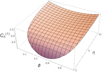


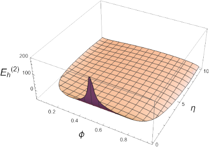


The plots are obtained by evaluating the analytic formulas at one and two loops with high precision on evenly spaced grid points. The numerical evaluation of the GPLs is carried out by HandyG Naterop:2019xaf (away from threshold) and Ginac Vollinga:2004sn (close to threshold) through their interface to PolyLogTools Duhr:2019tlz.
The finite term of the analytic expression of the two-loop contribution , which constitutes the main result of this communication, is found in agreement with the numerical results available in Czakon:2008zk.
In particular, the numerical values of the grid attached to the arXiv submission of the latter reference agree with the (higher accuracy) values obtained from the numerical evaluation of our analytic expressions, in the same phase-space points.
For completeness, the values of
, numerically evaluated at 1600 phase-space points,
are given in the ancillary file
qqQQGrid.m,
attached to this publication.
Our grid is given in the format , for the scale choice
,
in the same phase-space points chosen in Czakon:2008zk.
In Table 1, we showcase the numerical values of the analytic expressions of the individual colour factors, at one- and two-loop. The analytic expressions are evaluated with Ginac at the kinematic point , , (following the prescription given in eq.(27), the imaginary term is chosen to have ), which corresponds to the same kinematic point as in the Table 3 of Czakon:2008zk (see also Table 1 of Baernreuther:2013caa), and our results are in agreement up-to the digits reported in the latter.
Moreover, the analytic expressions of the finite part, as well as of the poles, of , , , , , agree with earlier results published in Bonciani:2008az; Bonciani:2009nb.
| - | - | - | - | -2 | ||
| - | - | 0.1026418456757775 | 1.356145770566065 | 2.230403451742140 | ||
| - | - | -0.3180868339485723 | -5.763132746701004 | 2.913169881363488 | ||
| - | - | 0 | 0 | -0.01726400752682416 | 1.235821434465827 | |
| - | - | 0 | 0 | -0.5623350683773134 | 0.6373589172648111 | |
| 1.391733154324222 | -2.298174307221209 | -4.145752448999165 | 17.37136598564062 | - | ||
| -1.323646320375650 | 8.507455541210568 | 6.035611156200398 | -35.12861106350758 | - | ||
| -0.06808683394857230 | -18.00716652035224 | 6.302454931016090 | 3.524044912826756 | - | ||
| 0 | - | 0.2605057338631945 | -0.7250180282219092 | -1.935417246635768 | - | |
| 0 | 0 | 0.5623350683773134 | 0.1045606449242690 | -1.704747997587188 | - | |
| 0 | -0.3323207299541260 | 7.904121951420471 | 2.848697836597635 | - | ||
| 0 | 0 | -0.5623350683773134 | 4.528240788258799 | 12.73232424278180 | - | |
| 0 | 0 | 0 | 0 | -1.984228442234312 | - | |
| 0 | 0 | 0 | 0 | -2.442562819239786 | - | |
| 0 | 0 | 0 | 0 | -0.07924540546146283 | - |
5 Conclusion
We completed the analytic evaluation of the scattering amplitude for the process at two loops in QCD, for a massless and a massive quark type. The contribution of the leading colour diagrams and of those containing fermion loops, whose analytical results were already available in the literature, were independently evaluated and cross checked, and combined with the novel contributions of the sub-leading colour terms, which were evaluated in this work, for the first time.
The un-renormalised interference terms of the one- and two-loop bare amplitudes with the leading-order one were computed in the framework of CDR. The renormalisation of the ultraviolet divergences was carried out by employing the on-shell scheme for the quarks, and the -scheme for the strong coupling constants.
The analytic results of the one- and two-loop renormalised contributions, obtained as Laurent series around dimensions, respectively, up-to the first order term, and up-to the finite term, were expressed in terms of GPLs and transcendental constants of up-to weight four. The singularity structure of the renormalised results was found to be in compliance with the predicted universal infrared behaviour of QCD amplitudes Becher:2009kw; Ferroglia:2009ep; Ferroglia:2009ii. Numerical and partial analytical results of the scattering amplitude already available in the literature Czakon:2008zk; Bonciani:2008az; Bonciani:2009nb; Baernreuther:2013caa agree with the novel analytic expression.
The analytic results of the two-loop scattering amplitude for the top-quark pair production from the light-quark annihilation channel are an essential ingredient to be combined with the ones of the gluon fusion channel, whose analytic knowledge is partially available Bonciani:2010mn; vonManteuffel:2013uoa; Bonciani:2013ywa; Adams:2018bsn; Adams:2018kez; Badger:2021owl, to obtain – hopefully, in a not-so-far future – the full analytic expressions of the scattering amplitudes for the production of a heavy quark-antiquark pair in hadron collisions, at two loops in QCD Czakon:2008zk; Baernreuther:2013caa.
The results presented for the process in QCD can be considered as an extension to the non-Abelian case of the ones recently obtained for the process in QED Bonciani:2021okt. The automatic framework which was developed for these calculations is flexible and applicable to other scattering reactions. The computational efforts and the intermediate results for the non-Abelian case, such as diagram generation, integral and integrand decompositions, and evaluation of master integrals, are ingredients that are now available for the study of the elastic scattering processes of one massless and one massive particle/body, which is related by crossing symmetry to the one presented here.
The competences acquired during this work, as well as the building blocks of the calculations, are not limited to applications within Particle Physics, and could be applied, for instance, to investigate processes in General Relativity, like the bending of light caused by a massive astrophysical body, see for instance Bjerrum-Bohr:2016hpa; Bjerrum-Bohr:2017dxw, where the massless quark is replaced by a photon, the massive quark is replaced by the world-line of a black-hole, and gluons are replaced by gravitons.
Let us finally remark that, more generally, the presented results constitute a crucial reference for the study of the scattering of particles/bodies with non-vanishing masses, for interactions mediated by self-interacting massless quanta, in the limiting case when one of the body can be treated as massless. Therefore, they can offer additional insights for investigating similarities and differences between fundamental interactions occurring in different physical scenarios.
Acknowledgements.
We wish to thank A. Primo for collaboration at early stage of this project, in particular, during the development of Aida and for discussions on the diagrams shown in Fig. 6. W.J.T. would like to thank J. Mazzitelli for suggesting numerical checks on the analytic expressions presented in this manuscript. We wish to acknowledge R. Bonciani, A. Broggio, M. Czakon, S. Di Vita, A. Ferroglia, F. Gasparotto, T. Gehrmann, M. Grazzini, A. Primo, U. Schubert, A. Signer, and F. Tramontano, for stimulating discussions at various stages, and comments on the manuscript. The work of M.K.M is supported by Fellini - Fellowship for Innovation at INFN funded by the European Union’s Horizon 2020 research and innovation programme under the Marie Skłodowska-Curie grant agreement No 754496. J.R. acknowledges support from INFN. This project received funding from the European Research Council (ERC) under the European Union’s Horizon 2020 research and innovation programme (grant agreement No 725110), Novel structures in scattering amplitudes.Appendix A Colour Stripped Form Factors
The Feynman diagrammatic approach has been adopted throughout the calculation, and in this Appendix, we provide details on the contribution of the one- and two-loop Feynman diagrams to the form factors present in decompositions (9) and (10), respectively.
In decomposition (9), for the one-loop contribution, we need to deal with 10 non-vanishing Feynman diagrams (see Fig. 2). Two of them contain vacuum polarisation insertions (with a closed heavy- and light-quark loop) contributing to form factors and . The remaining 8 diagrams may contribute to either (5 diagrams) or (4 diagrams). In particular, gets contribution from purely planar diagrams with and without self-gluon interactions. , and get contribution only from diagrams without self-gluon interactions.
Therefore, some of the form factors appearing in the decomposition of the considered amplitude, for a non-Abelian theory, can be written as linear combination of colour-stripped diagrams that would contribute to the scattering amplitude of an Abelian theory (like in QED). We list here, the decomposition of the form factors in terms of colour-stripped (Abelian-like) diagrams:
| (32) |
where accounts for colour-stripped -th Feynman diagram of Fig. 2.
Similarly, the form-factors appearing in decomposition of the two-loop amplitude in (10), gets contribution from 184 non-vanishing Feynman diagrams. In particular: gets contributions from 49 diagrams, which similarly to , are only planar; gets contributions from 62 (planar and non-planar) diagrams; gets contributions from 35 (planar and non-planar) diagrams; , from 19 diagrams; , from 20 diagrams; , from 15 diagrams; , from 15 diagrams; , from 1 diagram; , from 2 diagrams; and , from 1 diagrams.
In the same way, as in the one-loop decomposition, we notice that form factors , and get contributions from Feynman diagrams with and without self-gluon interactions, whereas, , and contain only diagrams without self-gluon interaction. Thus, the latter form factors can be decomposed in colour-stripped (Abelian-like) diagrams as:
| (33) | ||||
with stands for the colour-stripped -th Feynman diagram of Figs. 3 and 4.
Appendix B Renormalisation Constants
In this Appendix, we provide the expressions of the UV renormalisation constants introduced in Sec. 3.1, for convenience:
Light quark field:
| (34) | |||||
| (35) |
Heavy quark field and mass:
| (36) | |||||
| (37) | |||||
| (38) | |||||
Coupling constant:
| (39) | |||||
| (40) | |||||
where .
References
- (1) P. Nason, S. Dawson and R. K. Ellis, The Total Cross-Section for the Production of Heavy Quarks in Hadronic Collisions, Nucl. Phys. B303 (1988) 607.
- (2) W. Beenakker, H. Kuijf, W. L. van Neerven and J. Smith, QCD Corrections to Heavy Quark Production in p anti-p Collisions, Phys. Rev. D 40 (1989) 54–82.
- (3) W. Beenakker, W. L. van Neerven, R. Meng, G. A. Schuler and J. Smith, QCD corrections to heavy quark production in hadron hadron collisions, Nucl. Phys. B 351 (1991) 507–560.
- (4) P. Nason, S. Dawson and R. K. Ellis, The One Particle Inclusive Differential Cross-Section for Heavy Quark Production in Hadronic Collisions, Nucl. Phys. B 327 (1989) 49–92.
- (5) M. Czakon and A. Mitov, Inclusive Heavy Flavor Hadroproduction in NLO QCD: The Exact Analytic Result, Nucl. Phys. B 824 (2010) 111–135, [0811.4119].
- (6) P. Bärnreuther, M. Czakon and A. Mitov, Percent Level Precision Physics at the Tevatron: First Genuine NNLO QCD Corrections to , Phys. Rev. Lett. 109 (2012) 132001, [1204.5201].
- (7) M. Czakon and A. Mitov, NNLO corrections to top-pair production at hadron colliders: the all-fermionic scattering channels, JHEP 12 (2012) 054, [1207.0236].
- (8) M. Czakon and A. Mitov, NNLO corrections to top pair production at hadron colliders: the quark-gluon reaction, JHEP 01 (2013) 080, [1210.6832].
- (9) M. Czakon, P. Fiedler and A. Mitov, Total Top-Quark Pair-Production Cross Section at Hadron Colliders Through , Phys. Rev. Lett. 110 (2013) 252004, [1303.6254].
- (10) A. Gehrmann-De Ridder, T. Gehrmann and E. W. N. Glover, Antenna subtraction at NNLO, JHEP 09 (2005) 056, [hep-ph/0505111].
- (11) G. Abelof and A. Gehrmann-De Ridder, Antenna subtraction for the production of heavy particles at hadron colliders, JHEP 04 (2011) 063, [1102.2443].
- (12) G. Abelof, A. Gehrmann-De Ridder, P. Maierhofer and S. Pozzorini, NNLO QCD subtraction for top-antitop production in the channel, JHEP 08 (2014) 035, [1404.6493].
- (13) G. Abelof and A. Gehrmann-De Ridder, Light fermionic NNLO QCD corrections to top-antitop production in the quark-antiquark channel, JHEP 12 (2014) 076, [1409.3148].
- (14) G. Abelof, A. Gehrmann-De Ridder and I. Majer, Top quark pair production at NNLO in the quark-antiquark channel, JHEP 12 (2015) 074, [1506.04037].
- (15) M. Czakon, P. Fiedler and A. Mitov, Resolving the Tevatron Top Quark Forward-Backward Asymmetry Puzzle: Fully Differential Next-to-Next-to-Leading-Order Calculation, Phys. Rev. Lett. 115 (2015) 052001, [1411.3007].
- (16) M. Czakon, D. Heymes and A. Mitov, High-precision differential predictions for top-quark pairs at the LHC, Phys. Rev. Lett. 116 (2016) 082003, [1511.00549].
- (17) M. Czakon, P. Fiedler, D. Heymes and A. Mitov, NNLO QCD predictions for fully-differential top-quark pair production at the Tevatron, JHEP 05 (2016) 034, [1601.05375].
- (18) M. Czakon, D. Heymes and A. Mitov, fastNLO tables for NNLO top-quark pair differential distributions, 1704.08551.
- (19) M. Czakon, A novel subtraction scheme for double-real radiation at NNLO, Phys. Lett. B693 (2010) 259–268, [1005.0274].
- (20) M. Czakon, Double-real radiation in hadronic top quark pair production as a proof of a certain concept, Nucl. Phys. B 849 (2011) 250–295, [1101.0642].
- (21) M. Czakon and D. Heymes, Four-dimensional formulation of the sector-improved residue subtraction scheme, Nucl. Phys. B 890 (2014) 152–227, [1408.2500].
- (22) R. Bonciani, S. Catani, M. Grazzini, H. Sargsyan and A. Torre, The subtraction method for top quark production at hadron colliders, Eur. Phys. J. C 75 (2015) 581, [1508.03585].
- (23) S. Catani, S. Devoto, M. Grazzini, S. Kallweit and J. Mazzitelli, Top-quark pair production at the LHC: Fully differential QCD predictions at NNLO, JHEP 07 (2019) 100, [1906.06535].
- (24) S. Catani, S. Devoto, M. Grazzini, S. Kallweit, J. Mazzitelli and H. Sargsyan, Top-quark pair hadroproduction at next-to-next-to-leading order in QCD, Phys. Rev. D 99 (2019) 051501, [1901.04005].
- (25) S. Catani, S. Devoto, M. Grazzini, S. Kallweit and J. Mazzitelli, Top-quark pair hadroproduction at NNLO: differential predictions with the mass, JHEP 08 (2020) 027, [2005.00557].
- (26) S. Catani, S. Devoto, M. Grazzini, S. Kallweit and J. Mazzitelli, Bottom-quark production at hadron colliders: fully differential predictions in NNLO QCD, JHEP 03 (2021) 029, [2010.11906].
- (27) S. Catani and M. Grazzini, An NNLO subtraction formalism in hadron collisions and its application to Higgs boson production at the LHC, Phys. Rev. Lett. 98 (2007) 222002, [hep-ph/0703012].
- (28) W. J. Torres Bobadilla et al., May the four be with you: Novel IR-subtraction methods to tackle NNLO calculations, Eur. Phys. J. C 81 (2021) 250, [2012.02567].
- (29) G. Heinrich, Collider Physics at the Precision Frontier, Phys. Rept. 922 (2021) 1–69, [2009.00516].
- (30) S. Dittmaier, P. Uwer and S. Weinzierl, NLO QCD corrections to t anti-t + jet production at hadron colliders, Phys. Rev. Lett. 98 (2007) 262002, [hep-ph/0703120].
- (31) S. Dittmaier, P. Uwer and S. Weinzierl, Hadronic top-quark pair production in association with a hard jet at next-to-leading order QCD: Phenomenological studies for the Tevatron and the LHC, Eur. Phys. J. C 59 (2009) 625–646, [0810.0452].
- (32) S. Badger, M. Becchetti, E. Chaubey, R. Marzucca and F. Sarandrea, One-loop QCD helicity amplitudes for to , 2201.12188.
- (33) J. G. Korner, Z. Merebashvili and M. Rogal, NNLO results for heavy quark pair production in quark-antiquark collisions: The One-loop squared contributions, Phys. Rev. D 77 (2008) 094011, [0802.0106].
- (34) C. Anastasiou and S. M. Aybat, The One-loop gluon amplitude for heavy-quark production at NNLO, Phys. Rev. D 78 (2008) 114006, [0809.1355].
- (35) B. Kniehl, Z. Merebashvili, J. G. Korner and M. Rogal, Heavy quark pair production in gluon fusion at next-to-next-to-leading order: One-loop squared contributions, Phys. Rev. D 78 (2008) 094013, [0809.3980].
- (36) M. Czakon, Tops from Light Quarks: Full Mass Dependence at Two-Loops in QCD, Phys. Lett. B 664 (2008) 307–314, [0803.1400].
- (37) P. Bärnreuther, M. Czakon and P. Fiedler, Virtual amplitudes and threshold behaviour of hadronic top-quark pair-production cross sections, JHEP 02 (2014) 078, [1312.6279].
- (38) L. Chen, M. Czakon and R. Poncelet, Polarized double-virtual amplitudes for heavy-quark pair production, JHEP 03 (2018) 085, [1712.08075].
- (39) R. Bonciani, A. Ferroglia, T. Gehrmann, D. Maitre and C. Studerus, Two-Loop Fermionic Corrections to Heavy-Quark Pair Production: The Quark-Antiquark Channel, JHEP 07 (2008) 129, [0806.2301].
- (40) R. Bonciani, A. Ferroglia, T. Gehrmann and C. Studerus, Two-Loop Planar Corrections to Heavy-Quark Pair Production in the Quark-Antiquark Channel, JHEP 08 (2009) 067, [0906.3671].
- (41) R. Bonciani, A. Ferroglia, T. Gehrmann, A. von Manteuffel and C. Studerus, Two-Loop Leading Color Corrections to Heavy-Quark Pair Production in the Gluon Fusion Channel, JHEP 01 (2011) 102, [1011.6661].
- (42) A. von Manteuffel and C. Studerus, Massive planar and non-planar double box integrals for light Nf contributions to gg-tt, JHEP 10 (2013) 037, [1306.3504].
- (43) R. Bonciani, A. Ferroglia, T. Gehrmann, A. von Manteuffel and C. Studerus, Light-quark two-loop corrections to heavy-quark pair production in the gluon fusion channel, JHEP 12 (2013) 038, [1309.4450].
- (44) S. Badger, E. Chaubey, H. B. Hartanto and R. Marzucca, Two-loop leading colour QCD helicity amplitudes for top quark pair production in the gluon fusion channel, JHEP 06 (2021) 163, [2102.13450].
- (45) M. Czakon, A. Mitov and S. Moch, Heavy-quark production in gluon fusion at two loops in QCD, Nucl. Phys. B 798 (2008) 210–250, [0707.4139].
- (46) L. Adams, E. Chaubey and S. Weinzierl, Planar Double Box Integral for Top Pair Production with a Closed Top Loop to all orders in the Dimensional Regularization Parameter, Phys. Rev. Lett. 121 (2018) 142001, [1804.11144].
- (47) L. Adams, E. Chaubey and S. Weinzierl, Analytic results for the planar double box integral relevant to top-pair production with a closed top loop, JHEP 10 (2018) 206, [1806.04981].
- (48) M. Czakon, A. Mitov and S. Moch, Heavy-quark production in massless quark scattering at two loops in QCD, Phys. Lett. B 651 (2007) 147–159, [0705.1975].
- (49) P. Mastrolia, T. Peraro, A. Primo, J. Ronca and W. J. Torres Bobadilla, AIDA, Adaptive Integrand Decomposition Algorithm, .
- (50) P. Mastrolia, T. Peraro and A. Primo, Adaptive Integrand Decomposition in parallel and orthogonal space, JHEP 08 (2016) 164, [1605.03157].
- (51) P. Mastrolia, T. Peraro, A. Primo and W. J. Torres Bobadilla, Adaptive Integrand Decomposition, PoS LL2016 (2016) 007, [1607.05156].
- (52) T. Hahn, Generating Feynman diagrams and amplitudes with FeynArts 3, Comput. Phys. Commun. 140 (2001) 418–431, [hep-ph/0012260].
- (53) V. Shtabovenko, R. Mertig and F. Orellana, New Developments in FeynCalc 9.0, Comput. Phys. Commun. 207 (2016) 432–444, [1601.01167].
- (54) A. von Manteuffel and C. Studerus, Reduze 2 - Distributed Feynman Integral Reduction, 1201.4330.
- (55) P. Maierhfer, J. Usovitsch and P. Uwer, KiraA Feynman integral reduction program, Comput. Phys. Commun. 230 (2018) 99–112, [1705.05610].
- (56) S. Borowka, G. Heinrich, S. P. Jones, M. Kerner, J. Schlenk and T. Zirke, SecDec-3.0: numerical evaluation of multi-scale integrals beyond one loop, Comput. Phys. Commun. 196 (2015) 470–491, [1502.06595].
- (57) C. Duhr and F. Dulat, PolyLogTools — polylogs for the masses, JHEP 08 (2019) 135, [1904.07279].
- (58) J. Vollinga and S. Weinzierl, Numerical evaluation of multiple polylogarithms, Comput. Phys. Commun. 167 (2005) 177, [hep-ph/0410259].
- (59) L. Naterop, A. Signer and Y. Ulrich, handyG —Rapid numerical evaluation of generalised polylogarithms in Fortran, Comput. Phys. Commun. 253 (2020) 107165, [1909.01656].
- (60) T. Gehrmann and E. Remiddi, Differential equations for two loop four point functions, Nucl. Phys. B 580 (2000) 485–518, [hep-ph/9912329].
- (61) R. Bonciani, P. Mastrolia and E. Remiddi, Vertex diagrams for the QED form-factors at the two loop level, Nucl. Phys. B 661 (2003) 289–343, [hep-ph/0301170].
- (62) R. Bonciani, P. Mastrolia and E. Remiddi, Master integrals for the two loop QCD virtual corrections to the forward backward asymmetry, Nucl. Phys. B 690 (2004) 138–176, [hep-ph/0311145].
- (63) P. Mastrolia, M. Passera, A. Primo and U. Schubert, Master integrals for the NNLO virtual corrections to scattering in QED: the planar graphs, JHEP 11 (2017) 198, [1709.07435].
- (64) S. Di Vita, T. Gehrmann, S. Laporta, P. Mastrolia, A. Primo and U. Schubert, Master integrals for the NNLO virtual corrections to scattering in QCD: the non-planar graphs, JHEP 06 (2019) 117, [1904.10964].
- (65) M. Becchetti, R. Bonciani, V. Casconi, A. Ferroglia, S. Lavacca and A. von Manteuffel, Master Integrals for the two-loop, non-planar QCD corrections to top-quark pair production in the quark-annihilation channel, JHEP 08 (2019) 071, [1904.10834].
- (66) S. Catani, The Singular behavior of QCD amplitudes at two loop order, Phys. Lett. B 427 (1998) 161–171, [hep-ph/9802439].
- (67) G. F. Sterman and M. E. Tejeda-Yeomans, Multiloop amplitudes and resummation, Phys. Lett. B 552 (2003) 48–56, [hep-ph/0210130].
- (68) S. M. Aybat, L. J. Dixon and G. F. Sterman, The Two-loop soft anomalous dimension matrix and resummation at next-to-next-to leading pole, Phys. Rev. D 74 (2006) 074004, [hep-ph/0607309].
- (69) S. M. Aybat, L. J. Dixon and G. F. Sterman, The Two-loop anomalous dimension matrix for soft gluon exchange, Phys. Rev. Lett. 97 (2006) 072001, [hep-ph/0606254].
- (70) E. Gardi and L. Magnea, Factorization constraints for soft anomalous dimensions in QCD scattering amplitudes, JHEP 03 (2009) 079, [0901.1091].
- (71) E. Gardi and L. Magnea, Infrared singularities in QCD amplitudes, Nuovo Cim. C 32N5-6 (2009) 137–157, [0908.3273].
- (72) T. Becher and M. Neubert, Infrared singularities of scattering amplitudes in perturbative QCD, Phys. Rev. Lett. 102 (2009) 162001, [0901.0722].
- (73) T. Becher and M. Neubert, Infrared singularities of scattering amplitudes and N3LL resummation for -jet processes, JHEP 01 (2020) 025, [1908.11379].
- (74) T. Becher and M. Neubert, On the Structure of Infrared Singularities of Gauge-Theory Amplitudes, JHEP 06 (2009) 081, [0903.1126].
- (75) A. Mitov and S. Moch, The Singular behavior of massive QCD amplitudes, JHEP 05 (2007) 001, [hep-ph/0612149].
- (76) T. Becher and M. Neubert, Infrared singularities of QCD amplitudes with massive partons, Phys. Rev. D 79 (2009) 125004, [0904.1021].
- (77) A. Ferroglia, M. Neubert, B. D. Pecjak and L. L. Yang, Two-loop divergences of scattering amplitudes with massive partons, Phys. Rev. Lett. 103 (2009) 201601, [0907.4791].
- (78) A. Ferroglia, M. Neubert, B. D. Pecjak and L. L. Yang, Two-loop divergences of massive scattering amplitudes in non-abelian gauge theories, JHEP 11 (2009) 062, [0908.3676].
- (79) R. Bonciani et al., Two-Loop Four-Fermion Scattering Amplitude in QED, Phys. Rev. Lett. 128 (2022) 022002, [2106.13179].
- (80) J. Mazzitelli, P. F. Monni, P. Nason, E. Re, M. Wiesemann and G. Zanderighi, Top-pair production at the LHC with MiNNLOPS, 2112.12135.
- (81) ATLAS collaboration, G. Aad et al., Measurements of differential cross-sections in top-quark pair events with a high transverse momentum top quark and limits on beyond the Standard Model contributions to top-quark pair production with the ATLAS detector at TeV, 2202.12134.
- (82) M. L. Mangano, P. Nason and G. Ridolfi, Heavy quark correlations in hadron collisions at next-to-leading order, Nucl. Phys. B 373 (1992) 295–345.
- (83) J. G. Korner and Z. Merebashvili, One loop corrections to four point functions with two external massive fermions and two external massless partons, Phys. Rev. D 66 (2002) 054023, [hep-ph/0207054].
- (84) W. Bernreuther, A. Brandenburg, Z. G. Si and P. Uwer, Top quark pair production and decay at hadron colliders, Nucl. Phys. B 690 (2004) 81–137, [hep-ph/0403035].
- (85) G. ’t Hooft and M. J. G. Veltman, Regularization and Renormalization of Gauge Fields, Nucl. Phys. B44 (1972) 189–213.
- (86) C. G. Bollini and J. J. Giambiagi, Dimensional Renormalization: The Number of Dimensions as a Regularizing Parameter, Nuovo Cim. B12 (1972) 20–26.
- (87) C. Gnendiger et al., To , or not to : recent developments and comparisons of regularization schemes, Eur. Phys. J. C77 (2017) 471, [1705.01827].
- (88) K. G. Chetyrkin and M. Steinhauser, Short distance mass of a heavy quark at order , Phys. Rev. Lett. 83 (1999) 4001–4004, [hep-ph/9907509].
- (89) K. Melnikov and T. v. Ritbergen, The Three loop relation between the MS-bar and the pole quark masses, Phys. Lett. B 482 (2000) 99–108, [hep-ph/9912391].
- (90) K. Melnikov and T. van Ritbergen, The Three loop on-shell renormalization of QCD and QED, Nucl. Phys. B 591 (2000) 515–546, [hep-ph/0005131].
- (91) T. van Ritbergen, J. A. M. Vermaseren and S. A. Larin, The Four loop beta function in quantum chromodynamics, Phys. Lett. B 400 (1997) 379–384, [hep-ph/9701390].
- (92) M. Czakon, The Four-loop QCD beta-function and anomalous dimensions, Nucl. Phys. B 710 (2005) 485–498, [hep-ph/0411261].
- (93) P. A. Baikov, K. G. Chetyrkin and J. H. Kühn, Five-Loop Running of the QCD coupling constant, Phys. Rev. Lett. 118 (2017) 082002, [1606.08659].
- (94) T. Luthe, A. Maier, P. Marquard and Y. Schröder, Towards the five-loop Beta function for a general gauge group, JHEP 07 (2016) 127, [1606.08662].
- (95) F. Herzog, B. Ruijl, T. Ueda, J. A. M. Vermaseren and A. Vogt, The five-loop beta function of Yang-Mills theory with fermions, JHEP 02 (2017) 090, [1701.01404].
- (96) K. G. Chetyrkin, G. Falcioni, F. Herzog and J. A. M. Vermaseren, Five-loop renormalisation of QCD in covariant gauges, JHEP 10 (2017) 179, [1709.08541].
- (97) F. V. Tkachov, A Theorem on Analytical Calculability of Four Loop Renormalization Group Functions, Phys. Lett. B100 (1981) 65–68.
- (98) K. G. Chetyrkin and F. V. Tkachov, Integration by Parts: The Algorithm to Calculate beta Functions in 4 Loops, Nucl. Phys. B192 (1981) 159–204.
- (99) S. Laporta, High precision calculation of multiloop Feynman integrals by difference equations, Int. J. Mod. Phys. A15 (2000) 5087–5159, [hep-ph/0102033].
- (100) S. Di Vita, S. Laporta, P. Mastrolia, A. Primo and U. Schubert, Master integrals for the NNLO virtual corrections to scattering in QED: the non-planar graphs, JHEP 09 (2018) 016, [1806.08241].
- (101) J. M. Henn and W. J. Torres Bobadilla, Maximal transcendental weight contribution of scattering amplitudes, JHEP 03 (2022) 174, [2112.08900].
- (102) M. Argeri, S. Di Vita, P. Mastrolia, E. Mirabella, J. Schlenk, U. Schubert et al., Magnus and Dyson Series for Master Integrals, JHEP 03 (2014) 082, [1401.2979].
- (103) A. B. Goncharov, Multiple polylogarithms, cyclotomy and modular complexes, Math. Res. Lett. 5 (1998) 497–516, [1105.2076].
- (104) ATLAS Collaboration collaboration, G. Aad et al., Observation of a new particle in the search for the Standard Model Higgs boson with the ATLAS detector at the LHC, Phys.Lett. B716 (2012) 1–29, [1207.7214].
- (105) N. E. J. Bjerrum-Bohr, J. F. Donoghue, B. R. Holstein, L. Plante and P. Vanhove, Light-like Scattering in Quantum Gravity, JHEP 11 (2016) 117, [1609.07477].
- (106) N. E. J. Bjerrum-Bohr, B. R. Holstein, J. F. Donoghue, L. Planté and P. Vanhove, Illuminating Light Bending, PoS CORFU2016 (2017) 077, [1704.01624].