Two-qubit gate using conditional driving for highly detuned Kerr-nonlinear parametric oscillators Preprint: APS/123-QED

Hiroomi Chono Email: hiroomi1.chono@toshiba.co.jp Affiliation: Frontier Research Laboratory, Corporate Research & Development Center, Toshiba Corporation, 1, Komukai Toshiba-cho, Saiwai-ku, Kawasaki-shi, 212-8582, Japan Taro Kanao Affiliation: Frontier Research Laboratory, Corporate Research & Development Center, Toshiba Corporation, 1, Komukai Toshiba-cho, Saiwai-ku, Kawasaki-shi, 212-8582, Japan Hayato Goto Affiliation: Frontier Research Laboratory, Corporate Research & Development Center, Toshiba Corporation, 1, Komukai Toshiba-cho, Saiwai-ku, Kawasaki-shi, 212-8582, Japan

August 11, 2026

Abstract

A Kerr-nonlinear parametric oscillator (KPO) is one of the promising devices to realize qubits for universal quantum computing. The KPO can stabilize two coherent states with opposite phases, yielding a quantum superposition called a Schrödinger cat state. Universal quantum computing with KPOs requires three kinds of quantum gates: $R_{z},R_{x}$ , and $R_{zz}$ gates. We theoretically propose a two-qubit gate $R_{zz}$ for highly detuned KPOs. In the proposed scheme, we add a parametric drive for the first KPO. This leads to the $R_{zz}$ gate based on the driving of the second KPO depending on the first-KPO state, which we call “conditional driving.” First, we perform simulations using a conventional KPO Hamiltonian derived from a superconducting-circuit model under some approximations and evaluate the gate fidelity. Next, we also perform numerical simulations of the two-qubit gate using the superconducting-circuit model without the approximations. The simulation results indicate that the conditional-driving gates can be implemented with high fidelity ( $>99.9\%$ ) for rotation angles required for universality.

I INTRODUCTION

Superconducting circuits (SCs) are considered as a promising platform for implementing practical quantum computation Krantz et al. 2019; Kwon et al. 2021; Blais et al. 2021. The physical properties of superconducting qubits have garnered much attention since the first realization of a superconducting qubit about two decades ago Nakamura et al. 1997; Nakamura et al. 1999. Inspired by cavity quantum electrodynamics (QED) in atomic physics and quantum optics, circuit QED has also been developed Wallraff et al. 2004; Blais et al. 2004; Arute et al. 2019; Gong et al. 2021; Blais et al. 2021, and has improved technologies, such as qubit readout Wallraff et al. 2005, parametric amplifiers and oscillators Yamamoto et al. 2008; Lin et al. 2013; Lin et al. 2014, and various quantum-optics experiments Schuster et al. 2007; Kono et al. 2017.

Moreover, a charge-based superconducting qubit robust against stray electric field noise was proposed Koch et al. 2007; Schreier et al. 2008. The qubit is called a transmon, and it has become standard as a SC qubit. The transmon can be regarded as a nonlinear $LC$ circuit whose nonlinearity originates from Josephson junctions, and also as an anharmonic oscillator with the Kerr effect.

As a further development, a parametric oscillator formed by nonlinear $LC$ circuits whose Kerr nonlinearity is larger than the single-photon loss rate has been interested as a qubit, which is called a Kerr-nonlinear parametric oscillator (KPO) Goto 2016a; Goto 2016b; Goto 2019.

Although Kerr-nonlinear oscillators with/without parametric drive were theoretically studied more than two decades ago Milburn 1986; Miranowicz et al. 1990; Milburn and Holmes 1991; Leoński and Tanaś 1994; Leoński 1996; Ralph et al. 2003, the KPO has recently attracted intense attention again because of recent intriguing theoretical proposals for quantum annealing Goto 2016a; Goto 2019; Nigg et al. 2017; Puri et al. 2017a; Goto et al. 2018; Onodera et al. 2020; Goto and Kanao 2020; Kanao and Goto 2021 and gate-based quantum computing Goto 2016b; Puri et al. 2017b; Goto 2019; Puri et al. 2017a; Darmawan et al. 2021; Kwon et al. 2022; Kanao et al. 2022; Masuda et al. 2022; Mirrahimi et al. 2014.

A KPO can stabilize a quantum superposition of coherent states with opposite phase Goto 2016a; Goto 2016b; Puri et al. 2017b; Goto 2019; Puri et al. 2020; Darmawan et al. 2021, which is often called a Schrödinger cat state. A KPO is similar to a Josephson parametric oscillator (JPO) using a SC Lin et al. 2014. KPOs have been implemented experimentally with superconducting quantum interference devices (SQUIDs) Wang et al. 2019; Yamaji et al. 2022 or by a superconducting nonlinear asymmetric inductive element (SNAIL) transmon Grimm et al. 2020. For gate-based quantum computing using KPOs, three kinds of gates are required for universality: $R_{x}$ gate ( $X$ rotation), $R_{z}$ gate ( $Z$ rotation), and $R_{zz}$ gate ( $ZZ$ rotation) Goto 2016b; Puri et al. 2017b; Mirrahimi et al. 2014. The $R_{zz}$ gate can be realized by controlling a linear coupling between two KPOs Goto 2016b; Puri et al. 2017b. The single-qubit gates ( $R_{x},~R_{z}$ ) have been experimentally demonstrated, although the angle of one of them was limited, that is, not continuous Grimm et al. 2020. In contrast, the two-qubit gate ( $R_{zz}$ ) for KPOs has not been experimentally realized yet.

In this paper, we theoretically propose a two-qubit gate for highly detuned KPOs coupled with a fixed coupling rate. During idle time, the coupling between the KPOs is effectively turned off because of the large detuning between the KPOs. To perform a two-qubit gate, we add a parametric drive for the first KPO, the frequency of which is set to the sum of the KPO frequencies. This leads to the generation of photons with the second-KPO frequency through a three-wave mixing process in the first KPO, resulting in the driving of the second KPO depending on the first-KPO state, which we call “conditional driving.” The conditional driving is physically similar to the previously demonstrated cat-quadrature readout for a KPO Grimm et al. 2020. The $R_{zz}$ gate can be realized using the conditional driving induced by a gate pulse of the parametric drive, which we call the conditional-driving gate.

We propose a SC model of two coupled KPOs for the $R_{zz}$ gate and derive a simple model from the SC model under some approximations. Using these models, we show that high gate fidelity ( $>99.9~\%$ ) can be achieved for rotation angles required for universal quantum computing.

This paper is organized as follows. In Sec. II, we propose a two-qubit gate for highly detuned KPOs and show a SC for that. For simplicity, we start with the explanation of a single KPO and derive a conventional KPO Hamiltonian, which we call a simple model, from the SC model under some approximations. Next, we explain a SC model of the two-qubit gate for two coupled KPOs and derive a simple model under the same approximations. In Sec. III, using the simple and SC models, we demonstrate numerically that the $R_{zz}$ gate can be implemented with high fidelity. In Sec. IV, we investigate the effect of single-photon loss for the gate fidelity. Finally, we conclude this paper in Sec. V.

II Model

Refer to caption — Figure 1: Circuits of the two-qubit gate for KPOs using three-wave mixing (irradiated with the sum frequency). $\omega_{j}$ is the eigenfrequency of KPO $j~(j=1,2)$ .

II.1 $R_{zz}$ gate and SC

We propose the $R_{zz}$ gate for highly detuned KPOs. The proposed SC is shown in Fig. 1, where two KPOs are implemented as transmons with a dc-SQUID array Wang et al. 2019, and they are connected with a coupling capacitance. The frequencies of KPO1 and KPO2 are denoted by $\omega_{1}$ and $\omega_{2}$ , respectively. Because of the large detuning, the coupling between the two KPOs is effectively turned off during idle time. To perform the $R_{zz}$ gate, a parametric drive (flux modulation of the dc-SQUID array) for KPO1 with the sum frequency $\omega_{3}~(=\omega_{1}+\omega_{2})$ is added into the parametric drive with frequency of $2\omega_{1}$ , as shown in Fig. 1. Then, the two-mode squeezing between KPO1 and KPO2 is turned on, because of the three-wave mixing (Fig. 2) due to the nonlinearity of Josephson junctions in KPO1. The two-mode squeezing is known to be sufficient for realizing the $R_{zz}$ gate Xu et al. 2022. This process is also explained qualitatively as follows. The three-wave mixing leads to difference-frequency generation of a photon of $\omega_{2}=(\omega_{3}-\omega_{1})$ from a parametric pump photon of $\omega_{3}$ and a KPO1 photon of $\omega_{1}$ , as shown in Fig. 2. The photons of $\omega_{2}$ propagate to KPO2 via the coupling capacitance. Since the phase of the generated photons of $\omega_{2}$ depends on the phase of KPO1, the phase of KPO2 is rotated depending on the phase of KPO1, resulting in the $R_{zz}$ gate ( $ZZ$ rotation) Goto 2016b; Puri et al. 2017b; Goto 2019. (A more theoretical explanation is given in Sec. II.3.) We thus refer to this gate as a conditional-driving gate. We also investigate the $R_{zz}$ gate with a difference-frequency drive. (See Appendix B.)

II.2 Single KPO

Before discussing two KPOs, we explain the single-KPO case for simplicity. We also derive a simple model under some approximations, which is useful for parameter setting.

The SC of a KPO in Fig. 1 with a time-dependent external magnetic field proportional to $\theta_{0}-\delta_{p}\cos\omega_{p}t$ in the dc-SQUID array is governed by the following Hamiltonian Wang et al. 2019 (See Appendix A):

\hat{H}=4E_{C}\hat{n}^{2}-NE_{J}\cos(\theta_{0}-\delta_{p}\cos\omega_{p}t)\cos\frac{\hat{\varphi}}{N},

(1)

where $\omega_{p}$ is the parametric pump frequency ( $\omega_{p}=2\omega_{1}$ in Fig. 1), $N$ is the number of dc SQUIDs in the array, $E_{C}$ is the charging energy of shunt capacitance, $E_{J}$ is the Josephson energy, $\hat{n}$ and $\hat{\varphi}$ are the Cooper-pair number and phase-difference operators, respectively, satisfying the commutation relation $[\hat{\varphi},\hat{n}]=\textrm{i}$ . Equation (1) can be rewritten using bosonic operators $\hat{a}^{\dagger}$ and $\hat{a}$ as

\begin{split}\hat{H}&=\omega_{1}\hat{a}^{\dagger}\hat{a}-NE_{J}\cos(\theta_{0}-\delta_{p}\cos\omega_{p}t)\cos\frac{\hat{\varphi}}{N}\\ &\quad-NE_{J}\cos\theta_{0}\cdot\frac{\hat{\varphi}^{2}}{2N^{2}},\end{split}

(2)

where $\omega_{1}$ , $\hat{n}$ and $\hat{\varphi}$ are defined as

$\displaystyle\omega_{1}$	$\displaystyle=\left(\frac{8E_{C}\tilde{E}_{J}}{N}\right)^{\frac{1}{2}},$	(3)
$\displaystyle\hat{n}$	$\displaystyle=\textrm{i}\left(\frac{\tilde{E}_{J}}{32NE_{C}}\right)^{\frac{1}{4}}(\hat{a}^{\dagger}-\hat{a}),$
$\displaystyle\quad\hat{\varphi}$	$\displaystyle=\left(\frac{2NE_{C}}{\tilde{E}_{J}}\right)^{\frac{1}{4}}(\hat{a}^{\dagger}+\hat{a}),$

where $\tilde{E}_{J}~(=E_{J}\cos\theta_{0})$ is the effective Josephson energy.

Assuming a sufficiently small pump amplitude ( $\delta_{p}\ll 1$ ) and performing the rotating-wave approximation (RWA) in a rotating frame of half the pump frequency $\omega_{p}/2$ and in the transmon limit ( $E_{C}/E_{J}\ll 1$ ), we obtain the Hamiltonian in the simple model as

\hat{H}=\Delta\hat{a}^{\dagger}\hat{a}-\frac{K}{2}\hat{a}^{\dagger 2}\hat{a}^{2}+\frac{P}{2}(\hat{a}^{\dagger 2}+\hat{a}^{2}),

(4)

where $\Delta~(\simeq\omega_{1}-\omega_{p}/2)$ is the detuning, and the Kerr coefficient $K$ and the parametric pump amplitude $P$ are defined by

K=\frac{E_{C}}{N^{2}},\quad P=\delta_{p}\left(\frac{E_{C}\tilde{E}_{J}}{2N}\right)^{\frac{1}{2}}\tan\theta_{0}.

(5)

With the small amplitude the both models [Eqs. (1) and (4)] give approximately the same results as shown below. In this work, we set $\theta_{0}=\pi/4$ and $\Delta=0$ . The Hamiltonian in Eq. (4) has two degenerate eigenstates $\ket{\pm\alpha}$ with $\alpha=\sqrt{P/K}$ Puri et al. 2017b; Goto 2019, which are used as computational basis states.

We calculate the difference in average photon number between the SC and simple models for a single KPO. In Eq. (2), we set the pump frequency as $\omega_{p}=2\tilde{\omega}_{1}$ , where $\tilde{\omega}_{1}$ is the single-photon resonance frequency of KPO1 obtained by numerically diagonalizing $\hat{H}$ in Eq. (4). We also set the parameters as $E_{C}/h=300$ MHz, $P=4K$ , $\omega_{1}/2\pi=10$ GHz, and $N=5$ . The other parameters are obtained by their definitions such as Eqs. (3) and (5).

Figure 3 shows the dependence of the average photon numbers in the two models, where we solve the Schrödinger equation with $\delta_{p}(t)=\delta_{p,max}t/T$ , where $T$ is a sweeping time of $\delta_{p}$ . Figure 3(c) illustrates the difference between the two models. The photon number can be increased up to about 10 with a small amplitude such as $\delta_{p}=0.05$ in both models. In this region, $\delta_{p}$ is small enough to suppress the effect of the counter-rotating term, which was investigated in Masuda et al. 2021. The fast oscillations with small amplitudes in both models are due to nonadiabatic evolution. An even smaller oscillation is also shown in Fig. 3(c), which is probably due to fast oscillating terms dropped by the RWA.

II.3 Two coupled KPOs

The SC model of the two coupled KPOs shown in Fig. 1 is given by (see Appendix A for detail)

\begin{split}\hat{H}&=\sum_{j=1,2}\hat{H}_{j}+\hat{V},\\ \hat{H}_{1}&=\omega_{1}\hat{a}_{1}^{\dagger}\hat{a}_{1}-NE_{J1}\cos(\theta_{0}-\delta_{1}\cos\omega_{p1}t-\delta_{g}(t)\cos\omega_{3}t)\cos\frac{\hat{\varphi}_{1}}{N}-N\tilde{E}_{J1}\cdot\frac{\hat{\varphi}_{1}^{2}}{2N^{2}},\\ \hat{H}_{2}&=\omega_{2}\hat{a}_{2}^{\dagger}\hat{a}_{2}-NE_{J2}\cos(\theta_{0}-\delta_{2}\cos\omega_{p2}t)\cos\frac{\hat{\varphi}_{2}}{N}-N\tilde{E}_{J2}\cdot\frac{\hat{\varphi}_{2}^{2}}{2N^{2}},\\ \hat{V}&=\frac{16E_{C1}E_{C2}}{E_{C0}+E_{C1}+E_{C2}}\hat{n}_{1}\hat{n}_{2},\end{split}

(6)

where $\hat{H}_{j}$ is the Hamiltonian of KPO $j~(j=1,2)$ , $\delta_{j}$ and $\omega_{pj}$ are the parametric pump amplitude and frequency, respectively, for KPO $j$ , $E_{C0}$ is the charging energy for the coupling capacitor, $\delta_{g}$ is the amplitude of the gate pulse defined as

\begin{split}\delta_{g}(t)=p_{g0}\left(\frac{2N}{E_{C1}\tilde{E}_{J1}}\right)^{\frac{1}{2}}\frac{\tanh\tfrac{\beta t}{T_{g}}\tanh[\beta(1-\tfrac{t}{T_{g}})]}{\tanh^{2}\tfrac{\beta}{2}\tan\theta_{0}},\end{split}

(7)

where $p_{g0}$ and $T_{g}$ denote the peak value of the gate pulse and the gate time, respectively, and $\beta$ is a parameter determining the rise time of the gate pulse.

The Hamiltonian of the simple model is derived in a similar manner to the single-KPO case (See Appendix A for details):

\begin{split}\hat{H}&=\sum_{j=1,2}\hat{H}_{j}+\hat{H}_{\textrm{I}}+\hat{H}_{g},\\ \frac{\hat{H}_{j}}{\hbar}&=-\frac{K}{2}\hat{a}^{\dagger 2}_{j}\hat{a}^{2}_{j}+\frac{P}{2}\left(\hat{a}^{\dagger 2}_{j}+\hat{a}^{2}_{j}\right),\\ \frac{\hat{H}_{\textrm{I}}}{\hbar}&=g\left(\hat{a}_{1}\hat{a}^{\dagger}_{2}\textrm{e}^{-\textrm{i}\Delta_{12}t}+\hat{a}^{\dagger}_{1}\hat{a}_{2}\textrm{e}^{\textrm{i}\Delta_{12}t}\right),\\ \frac{\hat{H}_{g}}{\hbar}&=\frac{p_{g}(t)}{2}\left(\hat{a}^{2}_{1}\textrm{e}^{-\textrm{i}\Delta_{12}t}+\hat{a}^{\dagger 2}_{1}\textrm{e}^{\textrm{i}\Delta_{12}t}\right),\end{split}

(8)

where $g$ is a coupling constant (see Appendix A for its definition), $\Delta_{12}=\omega_{1}-\omega_{2}$ , $K$ and $P$ are given in the same manner as Eq. (5), and the gate pulse is given by

p_{g}(t)=p_{g0}\frac{\tanh\tfrac{\beta t}{T_{g}}\tanh[\beta(1-\tfrac{t}{T_{g}})]}{\tanh^{2}\tfrac{\beta}{2}}.

(9)

When $\Delta_{12}$ is sufficiently larger than any other parameters, the effect of $\hat{H}_{\textrm{I}}$ can be regarded as zero, since the factor $\textrm{e}^{-\textrm{i}\Delta_{12}t}$ oscillates very fast. By the gate pulse described by $\hat{H}_{g}$ , the parametric oscillation amplitudes of KPO1 become $\pm\alpha_{1}=\pm\sqrt{[P+p_{g}(t)\textrm{e}^{\textrm{i}\Delta_{12}t}]/K}$ . The second term with fast phase rotation corresponds to photons of $\omega_{2}$ generated by the difference frequency generation (three-wave mixing) in KPO1. This term cancels out the phase factor in $\hat{H}_{\textrm{I}}$ , resulting in turning on the coupling between the two KPOs. This is a mathematical explanation of the conditional driving. Thus, the $R_{zz}$ gate can be performed by the conditional driving induced by the gate pulse.

III $R_{zz}$ Gate simulations

In this section, we show the simulation results of the $R_{zz}$ gate using both the simple and SC models.

III.1 Simple model

Using the Hamiltonian in Eq. (8), we solve the Schrödinger equation to calculate time evolution of the two-KPO state $\ket{\psi}$ , and to evaluate the gate fidelity. For convenience, we introduce the following two state vectors:

\begin{split}&\Ket{\psi_{\textrm{even}}}\propto(\Ket{\alpha}\otimes\Ket{\alpha}+\Ket{-\alpha}\otimes\Ket{-\alpha}),\\ &\Ket{\psi_{\textrm{odd}}}\propto(\Ket{\alpha}\otimes\Ket{-\alpha}+\Ket{-\alpha}\otimes\Ket{\alpha}),\end{split}

(10)

where $\ket{\pm\alpha}$ are coherent states with $\alpha=\sqrt{P/K}$ . We set the initial and ideal final state as

	$\displaystyle\Ket{\psi(0)}$	$\displaystyle=\mathcal{N}_{0}(\Ket{\psi_{\textrm{even}}}+\Ket{\psi_{\textrm{odd}}}),$		(11)
	$\displaystyle\Ket{\psi_{\textrm{ideal}}(\Theta)}$	$\displaystyle=\mathcal{N}_{1}(\Ket{\Psi_{\textrm{even}}}+\textrm{e}^{\textrm{i}\Theta}\Ket{\Psi_{\textrm{odd}}}),$		(12)

where $\mathcal{N}_{0}$ and $\mathcal{N}_{1}$ are normalization factors, and

\Ket{\Psi_{\textrm{even}}}=\hat{U}_{0}(T_{g})\Ket{\psi_{\textrm{even}}},\quad\Ket{\Psi_{\textrm{odd}}}=\hat{U}_{0}(T_{g})\Ket{\psi_{\textrm{odd}}}.

(13)

Here we have introduced another rotating frame with the time-evolution operator $\hat{U}_{0}(t)$ without the gate pulse ( $\delta_{g}=0$ ) ¹¹ 1 This is a technique to extract the effect of the gate pulse, that is, to evaluate the fidelity between the actual state with the gate pulse and an ideal state with an ideal gate operation, where $\hat{U}_{0}$ (time-evolution operator without the gate pulse) plays a role of the effective identity operation.. From the definition of the $R_{zz}$ gate, the final state may be approximately given by

\begin{split}&\Ket{\psi(T_{g})}\simeq\alpha_{1}\Ket{\Psi_{\textrm{even}}}+\alpha_{2}\Ket{\Psi_{\textrm{odd}}},\\ &\alpha_{1}=\Braket{\Psi_{\textrm{even}}|\psi(T_{g})},\quad\alpha_{2}=\Braket{\Psi_{\textrm{odd}}|\psi(T_{g})}.\end{split}

(14)

Hence we define the rotation angle of the $R_{zz}$ gate as $\Theta=\theta_{2}-\theta_{1}$ , where $\theta_{1}$ and $\theta_{2}$ are the arguments of $\alpha_{1}$ and $\alpha_{2}$ , respectively. The gate fidelity of the $R_{zz}$ gate is thus defined by

F=|\Braket{\psi_{\textrm{ideal}}(\Theta)|\psi(T_{g})}|^{2}.

(15)

Figure 4(a) shows the simulation results of the gate fidelity using the simple model. We find that high fidelities over $99.9\%$ can be achieved for $\Theta$ in the range from $0$ to $\pi/2$ , which is sufficient for universality. (We have also investigated the $R_{zz}$ gate using a difference-frequency drive Darmawan et al. 2021, instead of the sum-frequency one, and also obtained high fidelities over $99.9\%$ . Interestingly, the fidelity is a little lower than in the case of the sum-frequency drive. See Appendix B for details.)

III.2 SC model

Next, we perform numerical simulations using the SC model. Using the Hamiltonian in Eq. (6), we solve the Schrödinger equation and evaluate the gate fidelity, where the initial state is set as Eq. (11). Using the ideal final state defined by Eq. (12) and the final state obtained by the simulation, the gate fidelity is also calculated by Eq. (15). Figure 4(b) shows the gate fidelity of the $R_{zz}$ gate in the SC model. The $R_{zz}$ gate can be performed with high fidelities over $99.9\%$ in the range from 0 to $\pi/2$ . [The gate fidelity using a SC model with the difference-frequency drive is shown in Fig. 7(b).]

IV Effect of single-photon loss

Figure 5: Infidelity of

R_{zz}

gate for the rotation angle

\pi/2

as a function of single-photon loss rate

T_{1}=\gamma^{-1}

using the simple model. The parameters are the same as in Sec. III A.

Finally, we study the effect of single-photon loss of KPOs, using the simple model. Taking the effect into account, the time evolution of the density operator $\hat{\rho}$ can be written by the following master equation:

\partial_{t}\hat{\rho}=-\frac{\textrm{i}}{\hbar}[\hat{H},\hat{\rho}]+\frac{\gamma}{2}\sum_{j=1,2}\left(2\hat{a}_{j}\hat{\rho}\hat{a}_{j}^{\dagger}-\hat{\rho}\hat{a}_{j}^{\dagger}\hat{a}_{j}-\hat{a}_{j}^{\dagger}\hat{a}_{j}\hat{\rho}\right),

(16)

where $\gamma$ is the single-photon loss rate ( $T_{1}^{-1}$ ) of KPOs. We evaluate the error rates of the $R_{zz}$ gate by solving the master equation with decay time $T_{1}=\gamma^{-1}$ from 1 $\mu$ s to 1 ms. Figure 5 shows the infidelity $1-F$ for the rotation angle $\Theta$ of $\pi/2$ as a function of $T_{1}$ , where the fidelity is calculated by

F=\braket{\psi_{\textrm{ideal}}(\Theta)|\hat{\rho}(T_{g})|\psi_{\textrm{ideal}}(\Theta)}.

(17)

The decay time in a recent experiment Grimm et al. 2020 is $T_{1}=15.5$ $\mu$ s, which corresponds to $1-F\sim 2\%$ in Fig. 5. Figure 5 also shows that the infidelity below 0.1 $\%$ will require a decay time of longer than 500 $\mu$ s. The error due to the single-photon loss can be decreased by shorting the gate time. On the other hand, the shorter the gate time is, the worse the gate fidelity becomes owing to nonadiabatic evolution. These two factors are in a trade-off relationship on the gate operation. An analysis of this relationship will be carried out in future work.

V CONCLUSION

In this paper, we have proposed the conditional-driving gate, which is an $R_{zz}$ gate using conditional driving for highly detuned KPOs.

We have also proposed a SC composed of two transmons with a dc-SQUID array (KPOs) coupled with a capacitor. Using the simple and SC models of the proposed SC, we have numerically demonstrated that the $R_{zz}$ gate can be performed with high fidelity ( $>99.9\%$ ) for rotation angles required for universal quantum computing. We have also examined the effect of single-photon loss. The result suggests that the error probability below 0.1% will require a decay time of longer than 500 $\mu$ s, which seems challenging but is expected to be realized in the future, suggested by recent experimental advances Wang et al. 2022. We expect that this simple scheme will be helpful toward the first realization of the two-qubit gate for KPOs.

Acknowledgements

We thank Y. Matsuzaki, S. Masuda, T. Ishikawa, and S. Kawabata for fruitful discussion. This paper is based on results obtained from a project, JPNP16007, commissioned by the New Energy and Industrial Technology Development Organization (NEDO), Japan.

Appendix A SC HAMILTONIAN OF TWO KPOs

The SC Hamiltonian of coupled two KPOs (see Fig. 1) in Eq. (6) is derived from the following Lagrangian:

\begin{split}\mathcal{L}&=T-U,\\ T&=\sum_{j=1,2}\frac{C_{j}}{2}\dot{\phi}_{j}^{2}+\frac{C_{0}}{2}(\dot{\phi}_{1}-\dot{\phi}_{2})^{2},\quad\\ &=\frac{1}{2}\bm{\dot{\phi}}^{t}M\bm{\dot{\phi}},\\ U&=-\sum_{j=1,2}NE_{Jj}\cos(\theta_{0}-\delta_{j}\cos\omega_{pj}t)\cos\frac{\varphi_{j}}{N},\end{split}

(18)

where $T$ and $U$ are the kinetic and potential energy, $C_{0}$ is the coupling capacitance, $C_{j}$ is the shunt capacitance, $\phi_{j}$ is the magnetic flux across the dc-SQUID array, $N$ is the number of dc SQUIDs in the array, $E_{Jj}$ is the Josephson energy for a single dc SQUID for KPO $j$ . Here the flux in the dc-SQUID array is modulated with the external magnetic field $\Phi_{\textrm{ex}}$ such as $\pi\Phi_{\textrm{ex}}/\Phi_{0}=\theta_{0}-\delta_{p}\cos\omega_{p}t$ ( $\Phi_{0}$ is the flux quantum). The kinetic energy can be rewritten in a compact form using the following flux vector and capacitance matrix:

\bm{\dot{\phi}}^{t}=(\dot{\phi}_{1},\dot{\phi}_{2}),\quad M=\begin{pmatrix}C_{1}+C_{0}&-C_{0}\\ -C_{0}&C_{2}+C_{0}\end{pmatrix}.

(19)

The charge $Q_{j}$ , which is the canonical conjugate of $\phi_{j}$ , is given by $\bm{Q}=M\bm{\dot{\phi}},~[\bm{Q}^{t}=(Q_{1},Q_{2})]$ . From the Legendre transformation, we obtain the following Hamiltonian:

\begin{split}H&=\frac{1}{2}\bm{Q}^{t}M^{-1}\bm{Q}\\ &\quad-\sum_{j=1,2}NE_{Jj}\cos(\theta_{0}-\delta_{j}\cos\omega_{pj}t)\cos\frac{\varphi_{j}}{N}.\end{split}

(20)

Imposing quantization on the Hamiltonian, we obtain the quantum-mechanical Hamiltonian:

\begin{split}\hat{H}&=\hat{H}_{0}+\hat{V}\\ \hat{H}_{0}&=\frac{4E_{C1}(E_{C0}+E_{C2})\hat{n}_{1}^{2}+4E_{C2}(E_{C0}+E_{C1})\hat{n}_{2}^{2}}{E_{C0}+E_{C1}+E_{C2}}\\ &\quad-\sum_{j=1,2}NE_{Jj}\cos(\theta_{0}-\delta_{j}\cos\omega_{pj}t)\cos\frac{\hat{\varphi}_{j}}{N},\\ \hat{V}&=\frac{16E_{C1}E_{C2}}{E_{C0}+E_{C1}+E_{C2}}\hat{n}_{1}\hat{n}_{2},\end{split}

(21)

where $\hat{n}_{j},\hat{\varphi}_{j}$ are the Cooper-pair number and phase-difference operators satisfying the relation $[\hat{\varphi}_{i},\hat{n}_{j}]=\textrm{i}\delta_{i,j}$ . $E_{C0}~(E_{Cj})=e^{2}/2C_{0}~(e^{2}/2C_{j})$ is the charging energy of the corresponding capacitance. Substituting the following into Eq. (21),

\begin{split}\hat{n}_{j}&=\textrm{i}\left(\frac{\tilde{E}_{Jj}}{32NE_{Cj}}\right)^{\frac{1}{4}}(\hat{a}_{j}^{\dagger}-\hat{a}_{j}),\\ \quad\hat{\varphi}_{j}&=\left(\frac{2NE_{Cj}}{\tilde{E}_{Jj}}\right)^{\frac{1}{4}}(\hat{a}_{j}^{\dagger}+\hat{a}_{j}),\end{split}

(22)

we obtain Eq. (6). Performing the transmon approximation of $\cos(\hat{\varphi}_{j}/N)$ , we also obtain

\begin{split}\hat{H}_{0}&\approx\sum_{j=1,2}\frac{E_{C0}(E_{C1}+E_{C2})}{E_{C0}+E_{C1}+E_{C2}}\left(\frac{\tilde{E}_{Jj}}{2NE_{Cj}}\right)^{\frac{1}{2}}(\hat{a}_{j}^{\dagger}-\hat{a}_{j})^{2}+(E_{Jj}-\delta_{j}\cos\omega_{pj}t-\delta_{g}(t)\cos\omega_{3}t)\left(\frac{E_{Cj}}{2NE_{Jj}}\right)^{\frac{1}{2}}(\hat{a}_{j}^{\dagger}+\hat{a}_{j})^{2}\\ &\quad-\frac{E_{Cj}}{12N^{2}}(\hat{a}_{j}^{\dagger}+\hat{a}_{j})^{4},\\ \hat{V}&=-\underbrace{\frac{4E_{C1}E_{C2}}{E_{C0}+E_{C1}+E_{C2}}\left(\frac{\tilde{E}_{J1}\tilde{E}_{J2}}{4N^{2}E_{C1}E_{C2}}\right)^{\frac{1}{4}}}_{\displaystyle{g}}(\hat{a}_{1}^{\dagger}-\hat{a}_{1})(\hat{a}_{2}^{\dagger}-\hat{a}_{2}).\end{split}

(23)

Performing the RWA in a frame rotating at half the pump frequencies, we can obtain the Hamiltonian in Eq. (8).

Appendix B $R_{zz}$ GATE USING DIFFERENCE-FREQUENCY DRIVE

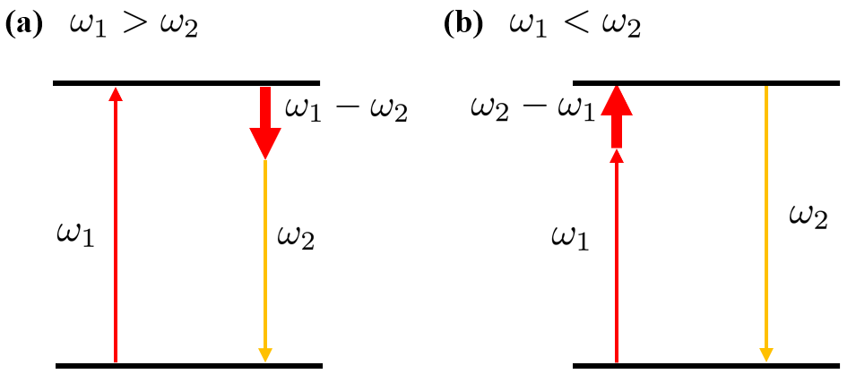
We also investigate the $R_{zz}$ gate using the difference-frequency drive, instead of the sum-frequency drive explained in the main text. In this case, the three-wave mixing process generating photons of $\omega_{2}$ differs depending on whether $\omega_{1}>\omega_{2}$ or $\omega_{2}>\omega_{1}$ . The generation processes are shown in Fig. 6. As shown in Fig. 6(a), when $\omega_{1}>\omega_{2}$ , photons of $\omega_{2}$ are generated by difference-frequency generation with the gate pulse of $\omega_{1}-\omega_{2}$ and photons of $\omega_{1}$ in KPO1. On the other hand, when $\omega_{2}>\omega_{1}$ , the photons of $\omega_{2}$ are generated by sum-frequency generation with them in Fig. 6(b).

In the case of the difference-frequancy drive, the Hamiltonian in the SC model is also given by Eq. (6), but in the simple model, $\hat{H}_{g}$ in Eq. (8) must be replaced by

\begin{split}\hat{H}_{g}=\frac{p_{g}(t)}{2}\cos(\Delta_{12}t)\hat{a}^{\dagger}_{1}\hat{a}_{1}.\end{split}

(24)

This Hamiltonian describes both difference-frequency and sum-frequency generations shown in Figs. 6(a) and 6(b), respectively, because $\cos(\Delta_{12}t)$ has both $\textrm{e}^{\textrm{i}\Delta_{12}t}$ and $\textrm{e}^{-\textrm{i}\Delta_{12}t}$ .

The simulation results of the $R_{zz}$ gate in the simple and SC models are shown in Fig. 7. It is found that we can also achieve high fidelities over $99.9\%$ using the difference-frequency drive.

References

Krantz et al. (2019) P. Krantz, M. Kjaergaard, F. Yan, T. P. Orlando, S. Gustavsson, and W. D. Oliver, A quantum engineer’s guide to superconducting qubits, Appl. Phys. Rev. 6, 021318 (2019).
Kwon et al. (2021) S. Kwon, A. Tomonaga, G. Lakshmi Bhai, S. J. Devitt, and J.-S. Tsai, Gate-based superconducting quantum computing, J. Appl. Phys. 129, 041102 (2021).
Blais et al. (2021) A. Blais, A. L. Grimsmo, S. Girvin, and A. Wallraff, Circuit quantum electrodynamics, Rev. Mod. Phys. 93, 025005 (2021).
Nakamura et al. (1997) Y. Nakamura, C. D. Chen, and J. S. Tsai, Spectroscopy of energy-level splitting between two macroscopic quantum states of charge coherently superposed by josephson coupling, Phys. Rev. Lett. 79, 2328 (1997).
Nakamura et al. (1999) Y. Nakamura, Y. A. Pashkin, and J. Tsai, Coherent control of macroscopic quantum states in a single-cooper-pair box, Nature (London) 398, 786 (1999).
Wallraff et al. (2004) A. Wallraff, D. I. Schuster, A. Blais, L. Frunzio, R.-S. Huang, J. Majer, S. Kumar, S. M. Girvin, and R. J. Schoelkopf, Strong coupling of a single photon to a superconducting qubit using circuit quantum electrodynamics, Nature (London) 431, 162 (2004).
Blais et al. (2004) A. Blais, R.-S. Huang, A. Wallraff, S. M. Girvin, and R. J. Schoelkopf, Cavity quantum electrodynamics for superconducting electrical circuits: An architecture for quantum computation, Phys. Rev. A 69, 062320 (2004).
Arute et al. (2019) F. Arute, K. Arya, R. Babbush, D. Bacon, J. C. Bardin, R. Barends, R. Biswas, S. Boixo, F. G. Brandao, D. A. Buell, et al., Quantum supremacy using a programmable superconducting processor, Nature (London) 574, 505 (2019).
Gong et al. (2021) M. Gong, S. Wang, C. Zha, M.-C. Chen, H.-L. Huang, Y. Wu, Q. Zhu, Y. Zhao, S. Li, S. Guo, et al., Quantum walks on a programmable two-dimensional 62-qubit superconducting processor, Science 372, 948 (2021).
Wallraff et al. (2005) A. Wallraff, D. I. Schuster, A. Blais, L. Frunzio, J. Majer, M. H. Devoret, S. M. Girvin, and R. J. Schoelkopf, Approaching unit visibility for control of a superconducting qubit with dispersive readout, Phys. Rev. Lett. 95, 060501 (2005).
Yamamoto et al. (2008) T. Yamamoto, K. Inomata, M. Watanabe, K. Matsuba, T. Miyazaki, W. D. Oliver, Y. Nakamura, and J. Tsai, Flux-driven josephson parametric amplifier, Appl. Phys. Lett. 93, 042510 (2008).
Lin et al. (2013) Z. Lin, K. Inomata, W. Oliver, K. Koshino, Y. Nakamura, J. Tsai, and T. Yamamoto, Single-shot readout of a superconducting flux qubit with a flux-driven josephson parametric amplifier, Appl. Phys. Lett. 103, 132602 (2013).
Lin et al. (2014) Z. Lin, K. Inomata, K. Koshino, W. Oliver, Y. Nakamura, J.-S. Tsai, and T. Yamamoto, Josephson parametric phase-locked oscillator and its application to dispersive readout of superconducting qubits, Nat. Commun. 5, 4480 (2014).
Schuster et al. (2007) D. Schuster, A. A. Houck, J. Schreier, A. Wallraff, J. Gambetta, A. Blais, L. Frunzio, J. Majer, B. Johnson, M. Devoret, et al., Resolving photon number states in a superconducting circuit, Nature (London) 445, 515 (2007).
Kono et al. (2017) S. Kono, Y. Masuyama, T. Ishikawa, Y. Tabuchi, R. Yamazaki, K. Usami, K. Koshino, and Y. Nakamura, Nonclassical photon number distribution in a superconducting cavity under a squeezed drive, Phys. Rev. Lett. 119, 023602 (2017).
Koch et al. (2007) J. Koch, M. Y. Terri, J. Gambetta, A. A. Houck, D. I. Schuster, J. Majer, A. Blais, M. H. Devoret, S. M. Girvin, and R. J. Schoelkopf, Charge-insensitive qubit design derived from the cooper pair box, Phys. Rev. A 76, 042319 (2007).
Schreier et al. (2008) J. Schreier, A. A. Houck, J. Koch, D. I. Schuster, B. Johnson, J. Chow, J. M. Gambetta, J. Majer, L. Frunzio, M. H. Devoret, et al., Suppressing charge noise decoherence in superconducting charge qubits, Phys. Rev. B 77, 180502 (2008).
Goto (2016a) H. Goto, Bifurcation-based adiabatic quantum computation with a nonlinear oscillator network, Sci. Rep. 6, 21686 (2016a).
Goto (2016b) H. Goto, Universal quantum computation with a nonlinear oscillator network, Phys. Rev. A 93, 050301(R) (2016b).
Goto (2019) H. Goto, Quantum computation based on quantum adiabatic bifurcations of Kerr-nonlinear parametric oscillators, J. Phys. Soc. Jpn. 88, 061015 (2019).
Milburn (1986) G. J. Milburn, Quantum and classical liouville dynamics of the anharmonic oscillator, Phys. Rev. A 33, 674 (1986).
Miranowicz et al. (1990) A. Miranowicz, R. Tanas, and S. Kielich, Generation of discrete superpositions of coherent states in the anharmonic oscillator model, Quantum Optics: Journal of the European Optical Society Part B 2, 253 (1990).
Milburn and Holmes (1991) G. J. Milburn and C. A. Holmes, Quantum coherence and classical chaos in a pulsed parametric oscillator with a kerr nonlinearity, Phys. Rev. A 44, 4704 (1991).
Leoński and Tanaś (1994) W. Leoński and R. Tanaś, Possibility of producing the one-photon state in a kicked cavity with a nonlinear kerr medium, Phys. Rev. A 49, R20 (1994).
Leoński (1996) W. Leoński, Fock states in a kerr medium with parametric pumping, Phys. Rev. A 54, 3369 (1996).
Ralph et al. (2003) T. C. Ralph, A. Gilchrist, G. J. Milburn, W. J. Munro, and S. Glancy, Quantum computation with optical coherent states, Phys. Rev. A 68, 042319 (2003).
Nigg et al. (2017) S. E. Nigg, N. Lörch, and R. P. Tiwari, Robust quantum optimizer with full connectivity, Sci. Adv. 3, e1602273 (2017).
Puri et al. (2017a) S. Puri, C. K. Andersen, A. L. Grimsmo, and A. Blais, Quantum annealing with all-to-all connected nonlinear oscillators, Nat. Commun. 8, 15785 (2017a).
Goto et al. (2018) H. Goto, Z. Lin, and Y. Nakamura, Boltzmann sampling from the Ising model using quantum heating of coupled nonlinear oscillators, Sci. Rep. 8, 7154 (2018).
Onodera et al. (2020) T. Onodera, E. Ng, and P. L. McMahon, A quantum annealer with fully programmable all-to-all coupling via Floquet engineering, npj Quantum Inf. 6, 48 (2020).
Goto and Kanao (2020) H. Goto and T. Kanao, Quantum annealing using vacuum states as effective excited states of driven systems, Commun. Phys. 3, 235 (2020).
Kanao and Goto (2021) T. Kanao and H. Goto, High-accuracy Ising machine using Kerr-nonlinear parametric oscillators with local four-body interactions, npj Quantum Inf. 7, 18 (2021).
Puri et al. (2017b) S. Puri, S. Boutin, and A. Blais, Engineering the quantum states of light in a Kerr-nonlinear resonator by two-photon driving, npj Quantum Inf. 3, 18 (2017b).
Darmawan et al. (2021) A. S. Darmawan, B. J. Brown, A. L. Grimsmo, D. K. Tuckett, and S. Puri, Practical quantum error correction with the XZZX code and kerr-cat qubits, PRX Quantum 2, 030345 (2021).
Kwon et al. (2022) S. Kwon, S. Watabe, and J.-S. Tsai, Autonomous quantum error correction in a four-photon Kerr parametric oscillator, npj Quantum Inf. 8, 40 (2022).
Kanao et al. (2022) T. Kanao, S. Masuda, S. Kawabata, and H. Goto, Quantum gate for a Kerr nonlinear parametric oscillator using effective excited states, Phys. Rev. Applied 18, 014019 (2022).
Masuda et al. (2022) S. Masuda, T. Kanao, H. Goto, Y. Matsuzaki, T. Ishikawa, and S. Kawabata, Fast tunable coupling scheme of Kerr-nonlinear parametric oscillators based on shortcuts to adiabaticity, arXiv:2203.00226 (2022).
Mirrahimi et al. (2014) M. Mirrahimi, Z. Leghtas, V. V. Albert, S. Touzard, R. J. Schoelkopf, L. Jiang, and M. H. Devoret, Dynamically protected cat-qubits: a new paradigm for universal quantum computation, New J. Phys. 16, 045014 (2014).
Puri et al. (2020) S. Puri, L. St-Jean, J. A. Gross, A. Grimm, N. E. Frattini, P. S. Iyer, A. Krishna, S. Touzard, L. Jiang, A. Blais, et al., Bias-preserving gates with stabilized cat qubits, Sci. Adv. 6, eaay5901 (2020).
Wang et al. (2019) Z. Wang, M. Pechal, E. A. Wollack, P. Arrangoiz-Arriola, M. Gao, N. R. Lee, and A. H. Safavi-Naeini, Quantum dynamics of a few-photon parametric oscillator, Phys. Rev. X 9, 021049 (2019).
Yamaji et al. (2022) T. Yamaji, S. Kagami, A. Yamaguchi, T. Satoh, K. Koshino, H. Goto, Z. R. Lin, Y. Nakamura, and T. Yamamoto, Spectroscopic observation of the crossover from a classical duffing oscillator to a Kerr parametric oscillator, Phys. Rev. A 105, 023519 (2022).
Grimm et al. (2020) A. Grimm, N. E. Frattini, S. Puri, S. O. Mundhada, S. Touzard, M. Mirrahimi, S. M. Girvin, S. Shankar, and M. H. Devoret, Stabilization and operation of a Kerr-cat qubit, Nature (London) 584, 205 (2020).
Xu et al. (2022) Q. Xu, J. K. Iverson, F. G. S. L. Brandão, and L. Jiang, Engineering fast bias-preserving gates on stabilized cat qubits, Phys. Rev. Res. 4, 013082 (2022).
Masuda et al. (2021) S. Masuda, T. Ishikawa, Y. Matsuzaki, and S. Kawabata, Controls of a superconducting quantum parametron under a strong pump field, Sci. Rep. 11, 11459 (2021).
(45) This is a technique to extract the effect of the gate pulse, that is, to evaluate the fidelity between the actual state with the gate pulse and an ideal state with an ideal gate operation, where $\hat{U}_{0}$ (time-evolution operator without the gate pulse) plays a role of the effective identity operation.
Wang et al. (2022) C. Wang, X. Li, H. Xu, Z. Li, J. Wang, Z. Yang, Z. Mi, X. Liang, T. Su, C. Yang, et al., Towards practical quantum computers: transmon qubit with a lifetime approaching 0.5 milliseconds, npj Quant. Inf. 8, 3 (2022).