Inference over Radiative Transfer Models using Variational and Expectation Maximization Methods Thanks: Research partly funded by the ERC under the ERC-CoG-2014 project (grant agreement 647423) and the ERC-SyG-2019 USMILE project (grant agreement 855187), the Ministerio de Ciencia e Innovación project PID2019-106827GB-I00/AEI/10.13039/501100011033, and the projects TEC2016-77741-R, DPI2017-89867-C2-2-R, RTI2018-096765-A-I00, PID2019-109026RB-I00 and PID2019-105032GB-I00.

Notationally, an RTM $\mathbf{f}$ operating in forward mode generates a multidimensional reflectance/radiance observation (or effect) ${\bf e}\in\mathbb{R}^{D_{e}}$ as observed by the sensor given a multidimensional parameter state vector (or cause) ${\bf c}\in\mathbb{R}^{D_{c}}$, see Fig. 1. Running forward simulations yields a look-up-table (LUT) of input-output pairs, ${\mathcal{D}}=\{(\mathbf{c}_{i},\mathbf{e}_{i})\}_{i=1}^{n}$. Solving the inverse problem using machine learning implies learning the function $\mathbf{g}$ using ${\mathcal{D}}$, to return an estimate $\mathbf{c}_{*}$ each time a new satellite observation $\mathbf{e}_{*}$ is acquired.

Notationally, let us consider then the vector of effects ${\bf e}\in\mathbb{R}^{D_{e}}$ and vector of causes ${\bf c}\in\mathcal{C}\subseteq\mathbb{R}^{D_{c}}$, an RTM model represents the underlying mapping from ${\bf c}$ to ${\bf e}$, that we denote as ${\bf f}({\bf c}):\mathbb{R}^{D_{c}}\rightarrow\mathbb{R}^{D_{e}}$. The complete observation model is given by

where $\mathbf{I}$ is a unit $D_{e}\times D_{e}$ matrix. The observation model defines the likelihood function as

Note that by fixing ${\bf c}$, the conditional probability $p({\bf e}|{\bf c})$ is Gaussian, but as a function of ${\bf c}$ the likelihood is a highly non-linear function due to the dependence on the RTM with the causes, i.e. ${\bf f}({\bf c})$. We assume an Gaussian prior over ${\bf c}$’s,

where ${\bf m}\in\mathbb{R}^{D_{c}}$ and the $D_{c}\times D_{c}$ covariance matrix ${\bf S}$ are considered unknown. The posterior density given the observed data $\mathbf{e}$ over the causes can be expressed as

Our goals are: (a) learn the prior parameters, vector ${\bf m}$ and matrix ${\bf S}$, and (b) obtain an approximation of the posterior $p({\bf c}|{\bf e})$, which serves as an inverse probabilistic mapping from ${\bf e}$ to ${\bf c}$. We assume that some set of data $\mathbf{e}$ is given. The two main ways of approaching this problem are a Variational inference (VI²² 2 Please note that we use VI to abbreviate variational inference as in most machine learning literature. This is not be confused with the abbreviation of vegetation indices in the remote sensing literature.) scheme on the one hand, and an expected maximization method on the other. For the VI method we follow the approach of Kingma and Welling kingma2013auto and substitute the decoder network with the generative model of Eq. (1). For the MC-based approach we use MC Expectation Maximization wei1990monte.

The idea of variational inference is to optimize the parameters of a variational posterior in order to come as close as possible to the true posterior. Following kingma2013auto we choose a Gaussian variational posterior,

where ${\bm{\mu}}_{\text{NN}}(\mathbf{e})$ and $\mathbf{\Sigma}_{\text{NN}}(\mathbf{e})$ are obtained by tuning a Neural Network (NN) with parameters ${\bm{\phi}}$. These parameters ${\bm{\phi}}$ are also referred to as the variational parameters. In order to tune the NN parameters ${\bm{\phi}}$, we minimize the Kullback-Leibler (KL) divergence between $q(\mathbf{c}|\mathbf{e})$ and the true posterior $p(\mathbf{c}|\mathbf{e})$, i.e.,

where we have used $\mathbb{E}_{q(\mathbf{c}|\mathbf{e})}[\log p(\mathbf{e})]=\log p(\mathbf{e})$. Since $\log p(\mathbf{e})$ is constant w.r.t. the variational parameters, in order to minimize the KL divergence, we have to maximize

called the Evidence Lower Bound (ELBO). We can split the ELBO into two terms: the first one represents the expected log-likelihood with respect to the variational posterior and the second one is the KL divergence between the variational posterior and the prior, i.e.,

As opposed to the approach in kingma2013auto we place a deterministic forward model in stead of a decoder network and fix a low value of noise variance in the likelihood (Eq. 2) in order to reflect the trust in the forward model. This approach is akin to that of mccarthy2017variational. In order to optimize this expression, we perform a Monte Carlo estimation of the expected value (i.e, the fist term) robert2013monte. The second term has a simple analytical form as it is the KL divergence between two Gaussians.

Importantly, maximizing $\mathcal{L}$ with respect to $\bm{\phi}$ should make $\mbox{KL}\left[q(\mathbf{c}|\mathbf{e})||p(\mathbf{c}|\mathbf{e})\right]$ fairly small and hence $\mathcal{L}\approx\log p(\mathbf{e})$. The maximization of $\mathcal{L}$ with respect to the prior parameters, $\bm{\theta}=\{\mathbf{m},\mathbf{S}\}$, is hence expected to maximize $\log p(\mathbf{e})$, which is the maximum likelihood principle for parameter estimation. In practice, we maximize $\mathcal{L}$ simultaneously with respect to $\bm{\theta}$ and $\bm{\phi}$.

The previous approach can be easily extended to the case of having several observed data instances $\{\mathbf{e}_{i}\}_{i=1}^{N}$. In that case the objective is simply the sum of $\mathcal{L}_{i}$, for $i=1,\ldots,N$, where $\mathcal{L}_{i}$ is the lower bound corresponding to $\mathbf{e}_{i}$, i.e., the $i$-th data instance. This sum can be approximated using mini-batches and optimized using stochastic optimization techniques such as the ADAM algorithm kingma2014adam. In this study, we use a mini-batch size of 1 for all experiments. For a proof of convergence of stochastic optimization see robbins1951stochastic. The variational approach is expected to find reasonable values for the prior parameters $\bm{\theta}$, using approximate maximum likelihood estimation, and to provide a recognition model $q(\mathbf{c}|\mathbf{e})$ that can be used to infer the potential values of $\mathbf{c}$ given $\mathbf{e}$.

Another method which can be used to address the learning goals described in Section 2, i.e. to infer the prior parameters from the observed data, and to generate samples from the posterior distribution $p(\mathbf{c}|\mathbf{e})$, is the Monte Carlo Expectation Maximization (MCEM) method wei1990monte.

We begin by briefly describing the Expectation Maximization (EM) algorithm, which can be used to maximize the likelihood function in models that involve latent variables dempster1977maximum. This is precisely the scenario considered in Section 2. Namely, given some observed data $\{\mathbf{e}_{i}\}_{i=1}^{N}$, we would like to maximize

as a function of the prior parameters ${\bm{\theta}}=\{\mathbf{m},\mathbf{S}\}$. Direct optimization of (8) is intractable, since we cannot marginalize the latent variables $\mathbf{c}_{i}$. The EM algorithm uses the fact that the complete likelihood function $p(\mathbf{e}_{i},\mathbf{c}_{i}|{\bm{\theta}})=p(\mathbf{e}_{i}|\mathbf{c}_{i})p(\mathbf{c}_{i}|{\bm{\theta}})$ is tractable. Consider the following decomposition of the logarithm of (8)

where we have introduced an approximate distribution $q_{i}(\mathbf{c}_{i})$ and

Note that (11) is the Kullback Leibler divergence between $q_{i}$ and the exact posterior $p(\mathbf{c}_{i}|\mathbf{e}_{i},{\bm{\theta}})$ for the instance $\mathbf{e}_{i}$.

The EM algorithm maximizes (9) in a two stage iterative process. Assume the current parameter vector is ${\bm{\theta}}^{\text{old}}$. In the E step, the lower bound $\sum_{i=1}^{N}\mathcal{L}(q_{i},{\bm{\theta}}^{\text{old}})$ is maximized with respect to each $q_{i}$ assuming ${\bm{\theta}}^{\text{old}}$ to be fixed. Because $\sum_{i=1}^{N}\log p(\mathbf{e}_{i}|{\bm{\theta}})$ does not depend on each $q_{i}$, the solution to this problem consists in setting each $q_{i}(\mathbf{c}_{i})$ equal to $p(\mathbf{c}_{i}|\mathbf{e}_{i},{\bm{\theta}}^{\text{old}})$, minimizing $\text{KL}(q_{i}||p_{i})$ in consequence. In the subsequent M step, each $q_{i}(\mathbf{c}_{i})$ is held fixed, and $\sum_{i=1}^{N}\mathcal{L}(q_{i},{\bm{\theta}}^{\text{old}})$ is maximized with respect to ${\bm{\theta}}$, to give new prior parameters ${\bm{\theta}}^{\text{new}}$. This will cause the lower bound $\sum_{i=1}^{N}\mathcal{L}(q_{i},{\bm{\theta}}^{\text{old}})$ to increase, which will in turn increase the log-likelihood $\sum_{i=1}^{N}\log p(\mathbf{e}_{i}|{\bm{\theta}})$. Critically, $q_{i}(\mathbf{c}_{i})$ will be computed in this step using ${\bm{\theta}}^{\text{old}}$, which is fixed. Therefore, the only required integral to evaluate in the M step is

A difficulty, however, is that the posterior $p(\mathbf{c}_{i}|\mathbf{e}_{i},{\bm{\theta}}^{\text{old}})$ is intractable, which makes computing $q_{i}$ and hence the integral in (12) challenging. Monte Carlo EM (MCEM), provides a solution to this problem wei1990monte. The intractable integral in (12) is simply approximated by a Monte Carlo average over several samples drawn from $q_{i}$. Namely,

where $\mathbf{c}_{i}^{s}$ has been generated from $q_{i}$ and $S$ is the number of generated samples. The convergence properties of MCEM are analyzed in neath2013convergence.

Recall that the approximate distribution $q_{i}$ is targeting the exact posterior $p(\mathbf{c}_{i}|\mathbf{e}_{i},{\bm{\theta}}^{\text{old}})$. So ideally, we should generate the samples $\mathbf{c}_{i}^{s}$ from the exact posterior. For this, we use Hamilton Monte Carlo (HMC) neal2011mcmc as in kingma2013auto. HMC is a Markov chain Monte Carlo (MCMC) method that can be used to generate (correlated) samples from some target distribution MartinoMh17. More specifically, a Markov chain is generated whose stationary distribution coincides with the target distribution. By running the Markov chain for a sufficiently large number of steps one can obtain an approximate independent sample from $p(\mathbf{c}_{i}|\mathbf{e}_{i},{\bm{\theta}}^{\text{old}})$. HMC has the advantage, when well-tuned, reduces substantially the correlation among samples MartinoMh17. For this, it simulates a dynamical system that uses information about the gradient of the posterior, i.e., $\nabla_{\mathbf{c}_{i}}\log p(\mathbf{c}_{i}|\mathbf{e}_{i},{\bm{\theta}}^{\text{old}})$, to sample from regions of high posterior probability. In our implementation of MCEM, the HMC procedure consists of 20 leapfrog steps with small step-size (i.e., $5\times 10^{-4}$) which guarantees that the acceptance rate is high enough. In practice, we only use just one sample to approximate (13). Each time, the Markov chain is initialized at the mode of the posterior distribution, which is found using quasi-newton optimization methods (i.e., L-BFGS). Of course, after optimizing the prior parameters ${\bm{\theta}}$ using MCEM, HMC can be used to generate samples from the approximate posterior distribution $\widehat{p}(\mathbf{c}|\mathbf{e},{\bm{\theta}})\propto p(\mathbf{e}|\mathbf{c})\widehat{p}_{{\bm{\theta}}}(\mathbf{c})$.

Note that both, the variational and MCEM methods, provide an estimation of the parameters ${\bm{\theta}}$ of the prior. Thus, we obtain a Gaussian approximation of the prior, which is denoted here as $\widehat{p}_{{\bm{\theta}}}(\mathbf{c})$. Therefore, both techniques provide the following posterior approximation

However, the variational algorithm provides another posterior approximation given in Eq.(5), i.e.,

which yields an important advantage with respect the previous one: given one $\mathbf{e}$, using $q(\mathbf{c}|\mathbf{e})$ we can easily, and at low computational cost, produce a predictive mean ${\bm{\mu}}_{\text{NN}}(\mathbf{e})$ and covariance $\mathbf{\Sigma}_{\text{NN}}(\mathbf{e})$. The approximation $\widehat{p}(\mathbf{c}|\mathbf{e},{\bm{\theta}})$ on the other hand would require the use of additional Monte Carlo schemes for obtaining a predictive mean and variance, for each new observation vector $\mathbf{e}$. Another advantage of the variational approach is the computational speed compared to the MCEM method. However, one advantage of the MCEM scheme is that it can directly handle more practical scenarios (e.g., problems involving multiple posterior modes, heavy tailed distributions, etc.) leading to better performance in terms of smaller error in the parameter estimation of the prior. The variational approach described here would require a different and more general derivation for addressing these scenarios, see e.g. mescheder2017adversarial. These features of each method are confirmed by the results obtained in our experiments. Implementations of the two approaches can be found at github.com/dhsvendsen/rtm_vi_mcem_inference.

In order to analyze the computational efficiency of the two approaches, we consider a simple forward model

for which both approaches converge to the true values of the parameters of the prior. We draw the training data $\{{\bf c}_{n}\}_{n=1}^{N}$ from the prior

and pass it through the nonlinear mapping ${\bf f}$ in order to generate the training data $\{\mathbf{e}_{n}\}_{n=1}^{N}$. Datasets of several sizes $N=\{50,500,1000,2000\}$ are used for training the models. The model likelihood noise is in all experiments fixed at a negligible value, with $\sigma^{2}=10^{-7}$, in order to reflect the trust in the knowledge encoded in the RTMs.

In Fig. 2 we plot an estimate of the average log marginal likelihood of each method on a test dataset as a function of training time (averaged over 40 repetitions). The marginal likelihood is computed using the estimator described in Appendix A. Observing the test log-likelihood, which is computed after each epoch, we see that the MCEM method convergences after 1 epoch (one iteration of the E and M steps). With a training dataset of 50 points, each epoch of training is sufficiently fast that a parallelized version of the MCEM method (in which each E step is done in parallel) converges faster than the VI method. For the non-parallelized algorithm, this is not the case. For larger datasets, VI converges before the completion of 1 epoch of the MCEM algorithm. Since this is a simple toy problem, larger learning rates can be used in the VI method, leading to earlier convergence (just after 1 epoch) for datasets of 1000 and 2000 points. We can conclude from these experiments that the VI approach (as a consequence of stochastic optimization) has a better scaling properties with respect to the dataset size than MCEM.

We have seen that when faced with sufficiently large amounts of training data, variational inference performs faster than Monte Carlo sampling methods. However, since the form of the variational posterior assumed in Eq. (5) is unimodal, we cannot expect it to be able to capture any multimodality in the true posterior. Consider for instance the forward mapping (with $\mathbf{c}=[c_{1},c_{2}]$),

For a given observed $\mathbf{e}=[e_{1},e_{2}]\geq[0,0]$ there will always be two possible solutions, namely $\mathbf{c}^{(1)}=[\sqrt{e_{1}},e_{2}/\sqrt{e_{1}}~]$ and $\mathbf{c}^{(2)}=[-\sqrt{e_{1}},-e_{2}/\sqrt{e_{1}}~]$ making the posterior inherently multimodal. As stated in the previous sections, we consider ${\bm{\epsilon}}\sim\mathcal{N}({\bm{\epsilon}}|{\bf 0},10^{-7}\mathbf{I})$. In this example, the prior density is Gaussian with parameters

from which $500$ samples are drawn and passed through $\mathbf{f}$ to generate the training dataset.

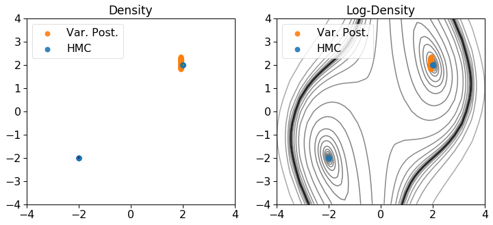
In the process of maximizing the ELBO, the expected log-likelihood with respect to the variational posterior is computed. We can see from Fig. 3, however, that the variational posterior, upon convergence, only captures the positive mode at $\mathbf{c}^{\prime}=[2,\,2]^{\top}$ of the true posterior given the observation $\mathbf{e}^{\prime}=[4,\,4]^{\top}$. On the other hand, the MCEM algorithm computes the expected complete log-likelihood with respect to the true posterior as approximated with HMC. As opposed to the variational posterior, HMC does manage to capture both the modes of the true posterior as shown in Fig. 3. The learning algorithm of the MCEM method is therefore more likely to converge to the true parameters of the prior if the posterior is multimodal.

We can see the inability of the variational method to capture the multimodality of the problem from the results of the converged methods given in Table 1. The fitted parameters of the prior are far from the true ones when compared to the results of the MCEM method which as also reflected in the KL divergence between the fitted and true prior distributions. Multimodality such as this is likely to be observed in the remote sensing experiment latter, as it has been remarked before that different configurations of inputs can lead to the same output making it an ill-posed inversion problem gomez2016efficient.

We now turn to inference in a remote sensing setting using one of the most widely used RTM over the last almost three decades in the field as our physical forward model jacquemoud2009prospect+. PROSAIL is a canopy reflectance model which allows us to relate fundamental vegetation canopy properties, such as, the Leaf Area Index (LAI), and leaf chemical and structural properties, to the scene reflectance for a given set of illumination and sensor (observation) geometry conditions liang2005quantitative. To perform its simulations, PROSAIL combines two sub-models: PROSPECT feret2008prospect, which models the optical properties of the leaves; and SAIL verhoef1984light, which models bidirectional reflectances considering the scattering by arbitrarily inclined canopy leaves in a turbid medium fang2019overview. This combination of models requires the following set of input parameters:

• 1)

  A set of leaf optical properties (PROSPECT), given by the mesophyll structural parameter (N), leaf chlorophyll (Chl), dry matter (Cm), water (Cw), carotenoid (Car) and brown pigment (Cbr) contents.

• 2)

  A set of canopy level and geometry characteristics (SAIL), determined by leaf area index (LAI), the average leaf angle inclination (ALA), the hot-spot parameter (Hotspot), the solar zenith angle ($\theta_{s}$), view zenith angle ($\theta_{v}$), and the relative azimuth angle between both angles ($\Delta\Theta$).

We consider PROSAIL for simulating Landsat-8 spectra. This satellite has been widely used in many applications such as cryosphere monitoring, aquatic science and surface water mapping, and vegetation monitoring wulder2019remote. Landsat 8’s Operational Land Imager (OLI) includes nine spectral bands with wavelengths ranging from $0.433\mu m$ to $1.390\mu m$, leaving us with an output-dimension of $D_{e}=9$ for our problem. In our experimental setup, we have chosen to work with the most relevant leaf-level parameters to monitor vegetation status and functioning included in PROSAIL, namely Cw, Cm and Chl, resulting in an input dimension of $D_{c}=3$. The remaining parameters were set constant during our experiments and their values were obtained from previous studies amogape20 to be representative of realistic cases. Their values can be found in Table 2.

Constraining the radiative transfer models with realistic and representative distributions of their inputs is a key part of the RTM inversion process. To facilitate this, in this work we relied on the largest global plant traits database available, the TRY database kattge2011try; kattge2020try, which contains thousands of leaf data records measured at unprecedented spatial and climatological coverage. Using these data we computed the following empirical mean vector and covariance matrix which was used to sample 2000 values of $\mathbf{c}$ and pass them through PROSAIL to generate the training data. The empirical mean and covariance (to be compared with the results in Table 3) of the samples are

The units of the parameters are g/cm² for Cm and Cw, and $\mu$g/cm² for Chl respectively. Note that the ground truth prior estimated from the TRY database has some probability density in the negative region of parameter space. This is not physically meaningful, but serves the point of illustrating the capabilities of the inference methods. We alter PROSAIL so that it sets every negative parameter to 0 before mapping into spectral space to get a modified likelihood that will lead to more multimodality (since all negative values in $\mathbf{c}$ will be mapped into the same value, i.e. 0, and then through PROSAIL into a spectrum).

The results of the variational approach to inference over PROSAIL are summarized in Fig. 4. We see that the parameters of the prior are fitted well, which can also be confirmed in Table 3 quantitatively, even though the variational posterior is not able to produce predictive means in the negative domain. It is interesting to note that the modification of PROSAIL to truncate negative data, which leads to multimodality, does not prevent the variational approach from estimating the parameters of the prior well.

Nevertheless, the MCEM method is somewhat more accurate than the VI method, obtaining a KL divergence with to the true prior of $1.23\times 10^{-2}$ compared to $2.08\times 10^{-2}$ obtained using the VI approach. This is to be expected since, as we have seen, the MCEM approach handles multimodality better. We especially foresee a clear difference in results in future work the LAI variable which is difficult to estimate due to its multimodal posterior distribution as pointed out elsewhere gomez2016efficient.

Once the VI method has converged, the neural network which parameterizes the variational posterior can be used as a fast inverse model that maps from observed satellite spectra to biophysical variables. Using the mean outputs that model the mean value of the variational posterior we can obtain good predictive accuracy on a test set as shown in the scatter plots of Fig. 5. Despite the promising results, it is very important to note that we run our experiments using a simplified PROSAIL configuration, keeping some of the input parameters static (see Table 2) and that results can vary greatly in more realistic modeling scenarios.

References

- (1) T.J. Santner, B.J. Williams, and W.I. Notz. The design and analysis of computer experiments. Springer Verlag, 2003.
- (2) B. Wescott. Every Computer Performance Book. Create Space Independent Publishing Platform, USA, 1st edition, 2013.
- (3) M. Raissi, P. Perdikaris, and G.E. Karniadakis. Machine learning of linear differential equations using Gaussian processes. Journal of Computational Physics, 348:683–693, Aug 2017.
- (4) A. Sandberg. Feasibility of whole brain emulation. In Philosophy and theory of artificial intelligence, pages 251–264. Springer, 2013.
- (5) D. H. Svendsen, L. Martino, and G. Camps-Valls. Active emulation of computer codes with Gaussian processes: Application to remote sensing. Pattern Recognition, 100:107103, 2020.
- (6) T. M. Lillesand, R. W. Kiefer, and J. Chipman. Remote Sensing and Image Interpretation. John Wiley & Sons, New York, 2008.
- (7) S. Liang. Advances in Land Remote Sensing: System, Modeling, Inversion and Applications. Springer Verlag, Germany, 2008.
- (8) C. D. Rodgers. Inverse Methods for Atmospheric Sounding: Theory and Practice. World Scientific Publishing Co. Ltd., 2000.
- (9) A. Tarantola. Inverse problem theory and methods for model parameter estimation, volume 89. siam, 2005.
- (10) D. H. Svendsen, L. Martino, M. Campos-Taberner, F. J. García-Haro, and G. Camps-Valls. Joint Gaussian Processes for biophysical parameter retrieval. IEEE Transactions on Geoscience and Remote Sensing, 56(3):1718–1727, 2018.
- (11) R. Zurita-Milla, V. Laurent, and J. van Gijsel. Visualizing the ill-posedness of the inversion of a canopy radiative transfer model: A case study for sentinel-2. International journal of applied earth observation and geoinformation, 43:7–18, 2015.
- (12) B. Combal, F. Baret, M. Weiss, A. Trubuil, D. Mace, A. Pragnere, R. Myneni, Y. Knyazikhin, and L. Wang. Retrieval of canopy biophysical variables from bidirectional reflectance: Using prior information to solve the ill-posed inverse problem. Remote sensing of environment, 84(1):1–15, 2003.
- (13) M. M. Verstraete and B. Pinty. Potential and limitations of information extraction the terrestrial biosphere from satellite remote sensing. Rem. Sens. Environ., 58:201–214, 1996.
- (14) Y. Knyazikhin. MODIS leaf area index (LAI), and fraction of photosynthetically active radiation absorbed by vegetation FPAR. Technical report, GSFC/NASA, http://eospso.gsfc.nasa.gov/atbd/modistables.html, 1999.
- (15) J. Vicent, L. Alonso, L. Martino, N. Sabater, J. Verrelst, G. Camps-Valls, and J. Moreno. Gradient-based Automatic Look-Up Table Generator for Radiative Transfer Models. IEEE Transactions on Geoscience and Remote Sensing, 57(2):1040–1048, 2019.
- (16) L. Liang, L. Di, L. Zhang, M. Deng, Z. Qin, S. Zhao, and H. Lin. Estimation of crop LAI using hyperspectral vegetation indices and a hybrid inversion method. Remote Sensing of Environment, 165:123–134, 2015.
- (17) M. Campos-Taberner, A. Moreno-Martínez, F. J. García-Haro, G. Camps-Valls, N. P. Robinson, J. Kattge, and S. W. Running. Global estimation of biophysical variables from google earth engine platform. Remote Sensing, 10(8):1167, 2018.
- (18) F. Baret et al. Lai, fapar and fcover cyclopes global products derived from vegetation: Part 1: Principles of the algorithm. Remote sensing of environment, 110(3):275–286, 2007.
- (19) N. Djamai, R. Fernandes, M. Weiss, H. McNairn, and K. Goïta. Validation of the sentinel simplified level 2 product prototype processor (sl2p) for mapping cropland biophysical variables using sentinel-2/msi and landsat-8/oli data. Remote sensing of environment, 225:416–430, 2019.
- (20) G. Camps-Valls, L. Martino, D. H. Svendsen, M. Campos-Taberner, J. Munoz-Mari, V. Laparra, D. Luengo, and J. Garcia-Haro. Physics-aware Gaussian Processes in remote sensing. Applied Soft Computing, 28:69–82, 2018.
- (21) G. Camps-Valls, J. Runge D. Sejdinovic, and M. Reichstein. A perspective on Gaussian processes for earth observation. National Science Review, 6:616–618, July 2019.
- (22) G. Camps-Valls, J. Verrelst, J. Muñoz Marí, V. Laparra, F. Mateo-Jiménez, and J. Gomez-Dans. A survey on Gaussian processes for earth observation data analysis. IEEE Geoscience and Remote Sensing Magazine, (6), June 2016.
- (23) B Pinty, I Andredakis, M Clerici, T Kaminski, M Taberner, MM Verstraete, N Gobron, S Plummer, and J-L Widlowski. Exploiting the modis albedos with the two-stream inversion package (jrc-tip): 1. effective leaf area index, vegetation, and soil properties. Journal of Geophysical Research: Atmospheres, 116(D9), 2011.
- (24) P Lewis, J Gómez-Dans, T Kaminski, Jeffrey Settle, Tristan Quaife, N Gobron, J Styles, and M Berger. An earth observation land data assimilation system (eo-ldas). Remote Sensing of Environment, 120:219–235, 2012.
- (25) C. Atzberger and K. Richter. Spatially constrained inversion of radiative transfer models for improved lai mapping from future sentinel-2 imagery. Remote Sensing of Environment, 120:208–218, 2012.
- (26) Cédric Bacour, Stéphane Jacquemoud, Marc Leroy, Olivier Hautecœur, Marie Weiss, Laurent Prévot, Nadine Bruguier, and Habiba Chauki. Reliability of the estimation of vegetation characteristics by inversion of three canopy reflectance models on airborne polder data. Agronomie, 22(6):555–565, 2002.
- (27) Qingyuan Zhang, Xiangming Xiao, Bobby Braswell, Ernst Linder, Fred Baret, and Berrien Moore III. Estimating light absorption by chlorophyll, leaf and canopy in a deciduous broadleaf forest using modis data and a radiative transfer model. Remote Sensing of Environment, 99(3):357–371, 2005.
- (28) Gabriele Coccia, Amanda L Siemann, Ming Pan, and Eric F Wood. Creating consistent datasets by combining remotely-sensed data and land surface model estimates through bayesian uncertainty post-processing: The case of land surface temperature from hirs. Remote Sensing of Environment, 170:290–305, 2015.
- (29) Chunfeng Ma, Xin Li, Claudia Notarnicola, Shuguo Wang, and Weizhen Wang. Uncertainty quantification of soil moisture estimations based on a bayesian probabilistic inversion. IEEE Transactions on Geoscience and Remote Sensing, 55(6):3194–3207, 2017.
- (30) G. C. G. Wei and M. A. Tanner. A Monte Carlo implementation of the EM algorithm and the poor man’s data augmentation algorithms. Journal of the American statistical Association, 85:699–704, 1990.
- (31) D. P. Kingma and M. Welling. Auto-encoding variational Bayes. arXiv preprint arXiv:1312.6114, 2013.
- (32) L. Mescheder, S. Nowozin, and A. Geiger. Adversarial variational Bayes: Unifying variational autoencoders and generative adversarial networks. In International Conference on Machine Learning, pages 2391–2400, 2017.
- (33) Frédéric Baret, Stéphane Jacquemoud, G Guyot, and C Leprieur. Modeled analysis of the biophysical nature of spectral shifts and comparison with information content of broad bands. Remote Sensing of Environment, 41(2-3):133–142, 1992.
- (34) Stéphane Jacquemoud and Frédéric Baret. Prospect: A model of leaf optical properties spectra. Remote sensing of environment, 34(2):75–91, 1990.
- (35) Wouter Verhoef. Light scattering by leaf layers with application to canopy reflectance modeling: The sail model. Remote sensing of environment, 16(2):125–141, 1984.
- (36) Adam McCarthy, Blanca Rodriguez, and Ana Mincholé. Variational inference over non-differentiable cardiac simulators using bayesian optimization. arXiv preprint arXiv:1712.03353, 2017.
- (37) Christian Robert and George Casella. Monte Carlo statistical methods. Springer Science & Business Media, 2013.
- (38) D. P. Kingma and J. Ba. ADAM: a method for stochastic optimization. In Inrernational Conference on Learning Representations, pages 1–15, 2015.
- (39) Herbert Robbins and Sutton Monro. A stochastic approximation method. The annals of mathematical statistics, pages 400–407, 1951.
- (40) A. P. Dempster, N. M. Laird, and D. B. Rubin. Maximum likelihood from incomplete data via the EM algorithm. Journal of the Royal Statistical Society: Series B (Methodological), 39:1–22, 1977.
- (41) R. C Neath. On convergence properties of the Monte Carlo EM algorithm. In Advances in modern statistical theory and applications: A festschrift in honor of Morris L. Eaton, pages 43–62. 2013.
- (42) R. M. Neal et al. MCMC using Hamiltonian dynamics. Handbook of Markov Chain Monte Carlo, 2(11):2, 2011.
- (43) L. Martino and V. Elvira. Metropolis sampling. Wiley StatsRef: Statistics Reference Online, pages 1–15, 2017.
- (44) José Luis Gómez-Dans, Philip Edward Lewis, and Mathias Disney. Efficient emulation of radiative transfer codes using Gaussian processes and application to land surface parameter inferences. Remote Sensing, 8(2):119, 2016.
- (45) S. Jacquemoud, W. Verhoef, F. Baret, C. Bacour, P.J. Zarco-Tejada, G.P. Asner, C. Francois, and S.L. Ustin. PROSPECT+ SAIL models: A review of use for vegetation characterization. Remote sensing of environment, 113:S56–S66, 2009.
- (46) S. Liang. Quantitative remote sensing of land surfaces, volume 30. John Wiley & Sons, 2005.
- (47) Jean-Baptiste Feret, Christophe Francois, Gregory P Asner, Anatoly A Gitelson, Roberta E Martin, Luc PR Bidel, Susan L Ustin, Guerric Le Maire, and Stéphane Jacquemoud. Prospect-4 and 5: Advances in the leaf optical properties model separating photosynthetic pigments. Remote sensing of environment, 112(6):3030–3043, 2008.
- (48) H. Fang, F. Baret, S. Plummer, and G. Schaepman-Strub. An overview of global leaf area index (lai): Methods, products, validation, and applications. Reviews of Geophysics, 57(3):739–799, 2019.
- (49) M. Wulder et al. Remote sensing of environment: Current status of landsat program, science, and applications. 2019.
- (50) Jens Kattge, Sandra Diaz, Sandra Lavorel, I Colin Prentice, Paul Leadley, Gerhard Bönisch, Eric Garnier, Mark Westoby, Peter B Reich, Ian J Wright, et al. Try–a global database of plant traits. Global change biology, 17(9):2905–2935, 2011.
- (51) Jens Kattge, Gerhard Bönisch, Sandra Díaz, Sandra Lavorel, Iain Colin Prentice, Paul Leadley, Susanne Tautenhahn, Gijsbert DA Werner, Tuomas Aakala, Mehdi Abedi, et al. Try plant trait database–enhanced coverage and open access. Global change biology.
- (52) M. Bugallo, L. Martino, and J. Corander. Adaptive importance sampling in signal processing. Digital Signal Processing, 47:36–49, 2015.
- (53) F. Llorente, L. Martino, D. Delgado, and J. Lopez-Santiago. Marginal likelihood computation for model selection and hypothesis testing: an extensive review. viXra:2001.0052, pages 1–58, 2019.
- (54) L. Martino, V. Elvira, D. Luengo, and J. Corander. Layered adaptive importance sampling. Statistics and Computing, 27(3):599–623, 2017.
Appendix A Marginal likelihood Estimation by Reverse Importance Sampling
In order to evaluate the performance of the methods described in the paper, we use a estimator of marginal likelihood on a test-dataset. More precisely, we use the Reverse Importance Sampling (RIS) estimator Llorente19ml described below:
- 1.
Sample values from the posterior with an MCMC-method. We use Hamiltonian Monte Carlo.
- 2.
Fit at density estimator to the samples . In this work we fit a Gaussian mixture model, doing cross validation in order to find the best number of components.
- 3.
Sample new values from the posterior to be inserted in the following estimator:
For the proof and more details see Llorente19ml. It is important to remark that the function must be a valid probability density for which there are several possible choices. If one chooses , RIS becomes the so-called harmonic mean estimator (this name is due to the fact that the corresponding estimator is the harmonic mean of the likelihood values). However, it has been shown that this does not lead to a good estimator. It is possible to show that, in order to ensure finite variance of the resulting estimator, the density should have equal or lighter tails than the posterior (e.g., see first numerical example in Llorente19ml). Gaussian mixture approximations and kernel density estimators of are suitable choices for . Different alternative estimators of the marginal likelihood are possible mixing MCMC and importance sampling schemes (see Llorente19ml; LAIS).