跳到论文正文
W Papers独立论文阅读器 arXiv:2204.03093 论文正文 计算阅读时间 · 0%
引用这篇论文根据当前论文元数据生成,正式投稿前建议核对。


License: arXiv.org perpetual non-exclusive license
arXiv:2204.03093v1 [gr-qc] 06 Apr 2022

Intertwiner Entanglement Excitation and Holonomy Operator

Qian Chen Email: chenqian.phys@gmail.com Affiliation: ENSL, CNRS, Laboratoire de Physique, F-69342 Lyon, France    Etera R. Livine Email: etera.livine@ens-lyon.fr Affiliation: ENSL, CNRS, Laboratoire de Physique, F-69342 Lyon, France
August 11, 2026
Abstract

In the loop quantum gravity framework, spin network states carries entanglement between quantum excitations of the geometry at different space points. This intertwiner entanglement is gauge-invariant and comes from quantum superposition of spins and intertwiners. Bipartite entanglement can be interpreted as a witness of distance, while multipartite entanglement reflects the curvature of the quantum geometry. The present work investigates how the bipartite and multipartite intertwiner entanglement changes under the action of the holonomy operator, which is the basic building block of loop quantum gravity’s dynamics. We reveal the relation between entanglement excitation and the dispersion of the holonomy operator. This leads to a new interesting connection between bulk geometry and boundary observables via the dynamics of entanglement.

I Introduction

Loop Quantum Gravity (LQG) proposes a background independent framework for a theory of quantum general relativity (see Gaul:1999ys; Thiemann:2007zz; Rovelli:2014ssa; Bodendorfer:2016uat for reviews), provides a local definition of quantum states of space geometry as spin networks and a canonical description for their dynamics through a Hamiltonian constraint. The geometry of 3d space slices is described by a pair of canonical fields, the (co-)triad and the Ashtekar-Barbero connection. Standard loop quantum gravity approach performs a canonical quantization of the holonomy-flux algebra, of observables smearing the Ashtekar-Barbero connection along 1d curves - holonomies, and the (co-)triad along 2d surfaces - fluxes, and defines quantum states of geometry as polymer structures or graph-like geometries with edges and vertices. Those spin network states represent the excitations of the Ashtekar-Barbero connection as Wilson lines in gauge field theory. On the other hand, geometric observables are raised to quantum operators acting on the Hilbert space spanned by spin networks, leading to the celebrated result of discrete spectra for areas (living along edges) and volumes (living at vertices) Rovelli:1994ge; Ashtekar:1996eg; Ashtekar:1997fb.

So spin networks are the kinematical states of the theory and the game is to describe their dynamics, i.e. their evolution in time generated by the Hamiltonian constraints11 1 Although the traditional canonical point of view is to attempt to discretize, regularize and quantize the Hamiltonian constraints Thiemann:1996aw; Thiemann:1996av, this often leads to anomalies. The formalism naturally evolved towards a path integral formulation. The resulting spinfoam models, constructed from (extended) topological quantum field theories (TQFTs) with defects, define transition amplitudes for histories of spin networks Reisenberger:1996pu; Baez:1997zt; Barrett:1997gw; Freidel:1998pt (see Livine:2010zx; Dupuis:2010kqh; Perez:2012wv for reviews). The formalism then evolves in a third quantization, where so-called “group field theories” define non-perturbative sums over random spin network histories in a similar way than matrix model partition functions define sums over random 2d discrete surfaces DePietri:1999bx; Reisenberger:2000zc; Freidel:2005qe (see Oriti:2006se; Carrozza:2013oiy; Oriti:2014yla for reviews). . Evolving spin networks, formalized as spinfoams, describe the four-dimensional quantum space-time at the Planck scale. This quantum space-time is defined without reference to a background classical geometry, with quantum states of geometry are defined up to diffeomorphisms with no reference to any intrinsic coordinate system or background structure. Then concepts in classical geometry, such as distance, area, curvature, become emergent notions, in a continuum limit after suitably coarse-graining Planck scale quantum fluctuations. They can only be reconstructed from the interaction between subsystems, quantified by correlation and entanglement shared between subsystems (see e.g. Donnelly:2016auv; Feller:2017jqx) For instance, bipartite correlations, equivalent to 2-point functions, allow to reconstruct a notion of distance while curvature should be reflected by multi-body correlations. This perspective sets the field of quantum information at the heart of research in quantum gravity, with essential roles to play for entanglement, decoherence and quantum localization in probing quantum states of geometries and thinking about the quantum-to-classical transition for the space-time geometry.

In the context of loop quantum gravity, the work investigating the entanglement carried by spin networks states have slowly built since the birth of the theory Livine:2005mw; Livine:2007sy; Donnelly:2008vx; Livine:2008iq; Donnelly:2011hn; Donnelly:2014gva; Feller:2015yta; Bianchi:2015fra; Feller:2016zuk; Bianchi:2016hmk; Delcamp:2016eya; Livine:2017fgq; Baytas:2018wjd, but has definitely sped up in the past few years with the burst of interest in the bulk-to-boundary propagator and bulk-from-boundary reconstruction in the light of holography, see for instance Anza:2016fix; Chirco:2017xjb; Colafranceschi:2021acz; Chirco:2021chk; Colafranceschi:2022ual. In this paper, we focus on intertwiner entanglement22 2 As shown in Livine:2017fgq, boundary state entanglement typically involves the gauge symmetry breaking and is defined with respect to gauge-variant physical measurements and the corresponding choice of boundary reference frame. On the other hand, intertwiner entanglement is gauge-invariant, and can be argued to quantify genuine spin network entanglement. , i.e. the entanglement between quanta of volume carried by a spin network state, and study the entanglement created by the holonomy operator, which is recognized both as a discretized measure of curvature in loop quantum gravity and as the basic building block of the Hamiltonian operator. We wish to understand how the excitation of curvature is related to the excitation of entanglement on spin network states. This is part of the larger line of research towards answering the questions: what is the relation between geometry and entanglement? Can one understand the dynamics of the quantum geometry directly in terms of evolution of entanglement and quantum information?

Furthermore, since the spin network is viewed as a many-body quantum system, it is necessary to introduce the notion of multipartite entanglement PhysRevA.68.042307; Amico:2007ag; GUHNE20091. It is still an ongoing topic in the field of quantum information. There are many candidates for quantifying the entanglement of multipartite system. These entanglement measures generally are not equivalent. In order to explore the entanglement structure for LQG, it is required to find a suitable entanglement measure. Our work shows that the notion of geometric measure of entanglement may be a good one, and justify the geometric measure since it admits a straightforward generalization from bipartite to multipartite spin network.

Section II sets up the mathematical definitions of the Hilbert space of spin network states, the defines and describes the action of the holonomy operator on those states. A gauge-invariant holonomy operator defined on a loop acts on all the intertwiner states living at the nodes of the spin network. Section III views spin network states as many-body quantum systems, living in the tensor product of the space of intertwiners attached to each node of the network. Spin network basis states, with fixed spins on the links and fixed intertwiners on the nodes, is a separable state and carries no entanglement. We explore the notion of multipartite entanglement PhysRevA.68.042307; Amico:2007ag; GUHNE20091 and define the notion of geometric entanglement for spin networks. Our main result is the computation of the growth of entanglement due to the action of the holonomy on a spin network basis state. Finally, sections IV and V apply this general result to the simplest network structures: the 2-vertex graph with boundary -or candy graph- consisting in two nodes and a triangular graph consisting in three nodes. These simple settings allow for explicit computations of the evolution (generated by the holonomy operator) of both the bipartite entanglement and the geometric multipartite entanglement, showing that they match at leading order.

II Holonomy operators on spin network Hilbert space

II.1 Spin network Hilbert space

Loop quantum gravity proceeds to a canonical quantization of general relativity (see Thiemann:2007zz for detailed lectures, or Ashtekar:2021kfp for a recent overview), describing the evolution of a 3d (space-like) slice in time, thereby generating the four-dimensional space-time. It defines quantum states of geometry and describes their constrained evolution in time. A state of geometry is defined as a wave-function ψ\psi of the Ashtekar-Barbero connection on the canonical hypersurface. Loop quantum gravity choose cylindrical wave-functions, that depend on the holonomies of that connection along the edges of a graph Γ\Gamma. These holonomies are SU⁡(2)\mathrm{SU}(2) group elements, ge∈SU⁡(2)g_{e}\in\mathrm{SU}(2) for each edge ee of the graph. And the wave-functions are required to be gauge-invariance under local SU⁡(2)\mathrm{SU}(2) transformations, which act at every vertices of the graph.

For closed 3d spatial slices, without boundary, we consider closed graphs, i.e. without open links. A wave-function ψ\psi on a closed oriented graph Γ\Gamma is a function of one SU⁡(2)\mathrm{SU}(2) group element geg_{e} for each edge ee, and is assumed to be invariant under the SU⁡(2)\mathrm{SU}(2)-action at each vertex vv of the graph:

ψΓ:SU​(2)×E⟶ℂ{ge}e∈Γ⟼ψ⁡({ge}e∈Γ)=ψΓ​({ht⁡(e)​ge​hs⁡(e)−1}e∈Γ),∀hv∈SU⁡(2)\begin{array}[]{rlcl}\psi_{\Gamma}:&\mathrm{SU}(2)^{\times E}&\longrightarrow&{\mathbb{C}}\\ &\{g_{e}\}_{e\in\Gamma}&\longmapsto&\psi(\{g_{e}\}_{e\in\Gamma})=\psi_{\Gamma}(\{h_{t(e)}g_{e}h_{s(e)}^{-1}\}_{e\in\Gamma})\,,\quad\forall h_{v}\in\mathrm{SU}(2)\end{array} (1)

where t⁡(e)t(e) and s⁡(e)s(e) respectively refer to the target and source vertices of the edge ee. We write EE and VV respectively for the number of edges and vertices of the considered graph Γ\Gamma. The scalar product between such wave-functions is given by the Haar measure on the Lie group SU⁡(2)\mathrm{SU}(2):

⟨ψΓ|ψ~Γ⟩=∫SU​(2)×E∏ed​ge​ψΓ​({ge}e∈Γ)¯​ψ~Γ​({ge}e∈Γ).\langle\psi_{\Gamma}|\widetilde{\psi}_{{\Gamma}}\rangle=\int_{\mathrm{SU}(2)^{{\times E}}}\prod_{e}\mathrm{d}g_{e}\,\overline{\psi_{\Gamma}(\{g_{e}\}_{e\in\Gamma})}\,\widetilde{\psi}_{{\Gamma}}(\{g_{e}\}_{e\in{\Gamma}})\,. (2)

The Hilbert space of quantum states with support on the closed graph Γ\Gamma is thus realized as a space of square-integrable functions, ℋΓ=L2​(SU​(2)×E/SU​(2)×V){\mathcal{H}}_{\Gamma}=L^{2}(\mathrm{SU}(2)^{{\times E}}/\mathrm{SU}(2)^{{\times V}}).

For a 3d slice with boundary, we consider graphs with open links puncturing the slice boundary. Those open links are connected to one vertex of the graph, while their other extremity is left loose. Without loss of generality, we can assume that all those open links are outward oriented, i.e. that their source vertex belongs to the graph, while their target vertex does not. Those open links are referred to as the boundary links. We can use the same definition as above for a closed graph, considering wave-functions of one group element per link, including both the standard links in the interior and the boundary links. The difference is that gauge transformations will only act at the graph vertices and will not act on the open ends.

Another way to proceed, as advocated in Chen:2021vrc, is to explicitly partition the graph set of edges into interior links and boundary links,

Γ=Γo⊔∂Γ.\Gamma=\Gamma^{o}\sqcup\partial\Gamma\,. (3)

One introduces the concept of boundary state as functions of the holonomies along the boundary links. Then one considers the bulk wave-functions as mapping holonomies along the interior links to boundary states:

ψΓ:SU(2){e∈Γo}⟶ℱ[SU(2){e∈∂Γ}]{ge}e∈Γo⟼ψ⁡[{ge}e∈Γo],\begin{array}[]{rlcl}\psi_{\Gamma}:&\mathrm{SU}(2)^{\{e\in\Gamma^{o}\}}&\longrightarrow&{\mathcal{F}}\big[\mathrm{SU}(2)^{\{e\in\partial\Gamma\}}\big]\\ &\{g_{e}\}_{e\in\Gamma^{o}}&\longmapsto&\psi[\{g_{e}\}_{e\in\Gamma^{o}}]\,,\end{array} (4)

with the bulk gauge invariance turning into a covariance property of the boundary states:

ψ⁡[{ge}e∈Γo]​({ge}e∈∂Γ)=ψ⁡[{ht⁡(e)​ge​hs⁡(e)−1}e∈Γo]​({ge​hs⁡(e)−1}e∈∂Γ),∀hv∈SU⁡(2).\psi[\{g_{e}\}_{e\in\Gamma^{o}}](\{g_{e}\}_{e\in\partial\Gamma})=\psi[\{h_{t(e)}g_{e}h_{s(e)}^{-1}\}_{e\in\Gamma^{o}}](\{g_{e}h_{s(e)}^{-1}\}_{e\in\partial\Gamma})\,,\quad\forall h_{v}\in\mathrm{SU}(2)\,. (5)

This follows the logic of state-sum models and discrete topological path integrals: boundary cells are dressed with quantum states, while bulk cells are dressed with morphisms of their boundary Hilbert space. When decomposing into spins, wave-functions on a closed graph can be decomposed on spin network states, dressed with one irreducible spin representation on each link jej_{e} and with one intertwiner state (or singlet state) on each vertex IvI_{v}. Wave-functions on an open graph can be similarly decomposed into bulk spin network states. In that case, as explained in Chen:2021vrc, the boundary Hilbert space is the tensor product of spin states living on the open links:

ℋ∂Γ=⨂e∈∂Γℋe,ℋe=⨁je∈ℕ2𝒱je.{\mathcal{H}}_{\partial\Gamma}=\bigotimes_{e\in\partial\Gamma}{\mathcal{H}}_{e}\,,\qquad{\mathcal{H}}_{e}=\bigoplus_{j_{e}\in\frac{{\mathbb{N}}}{2}}{\mathcal{V}}_{j_{e}}\,. (6)

A bulk state can be understood as a boundary map, i.e. a function from bulk group elements to the boundary Hilbert space:

ψ⁡[{ge}e∈Γo]∈ℋ∂Γ.\psi[\{g_{e}\}_{e\in\Gamma^{o}}]\in{\mathcal{H}}_{\partial\Gamma}\,. (7)

We refer the interested reader to Chen:2021vrc, and to the recent work Anza:2017dkd; Colafranceschi:2021acz; Colafranceschi:2022ual, for more details on wave-functions for bounded regions and interesting work on typical bulk states.

Let us now briefly review spin network states and notations. A basis of this Hilbert space can be constructed using the spin decomposition of L2L^{2} functions on the Lie group SU⁡(2)\mathrm{SU}(2) according to the Peter-Weyl theorem. A spin j∈ℕ2j\in\frac{{\mathbb{N}}}{2} defines an irreducible unitary representation of SU⁡(2)\mathrm{SU}(2), with the action of SU⁡(2)\mathrm{SU}(2) group elements realized on a (2​j+1)(2j+1)-dimensional Hilbert space 𝒱j{\mathcal{V}}_{j}. We use the standard orthonormal basis |j,m⟩|j,m\rangle, labeled by the spin jj and the magnetic index mm running by integer steps from −j-j to +j+j, which diagonalizes the SU⁡(2)\mathrm{SU}(2) Casimir J→2\vec{J}^{2} and the 𝔲⁡(1){\mathfrak{u}}(1) generator JzJ_{z}. Group elements gg are then represented by the (2​j+1)×(2​j+1)(2j+1)\times(2j+1) Wigner matrices Dj​(g)D^{j}(g):

Dm​m′j​(g)=⟨j,m​|g|​j,m′⟩,Dm​m′j​(g)¯=Dm′​mj​(g−1).D^{j}_{mm^{\prime}}(g)=\langle j,m|g|j,m^{\prime}\rangle\,,\qquad\overline{D^{j}_{mm^{\prime}}(g)}=D^{j}_{m^{\prime}m}(g^{-1})\,. (8)

These Wigner matrices form an orthogonal basis of L2​(SU​(2))L^{2}(\mathrm{SU}(2)):

∫SU⁡(2)d​g​Da​bj​(g)¯​Dc​dk​(g)=∫SU⁡(2)d​g​Db​aj​(g−1)¯​Dc​dk​(g)=δj​k2​j+1​δa​c​δb​d,δ⁡(g)=∑j∈ℕ2(2​j+1)​χj​(g),\int_{\mathrm{SU}(2)}\mathrm{d}g\,\overline{D^{j}_{ab}(g)}\,{D^{k}_{cd}(g)}=\int_{\mathrm{SU}(2)}\mathrm{d}g\,\overline{D^{j}_{ba}(g^{-1})}\,{D^{k}_{cd}(g)}=\frac{\delta_{jk}}{2j+1}\delta_{ac}\delta_{bd}\,,\qquad\delta(g)=\sum_{j\in\frac{{\mathbb{N}}}{2}}(2j+1)\chi_{j}(g)\,, (9)

where χj\chi_{j} is the spin-jj character defined as the trace of the Wigner matrix, χj​(g)=Tr​Dj​(g)=∑m=−jj⟨j,m​|g|​j,m⟩\chi_{j}(g)={\mathrm{Tr}}D^{j}(g)=\sum_{m=-j}^{j}\langle j,m|g|j,m\rangle. Applying this to gauge-invariant wave-functions allows to build the spin network basis states of ℋΓ{\mathcal{H}}_{\Gamma}, which depend on one spin jej_{e} on each edge and one intertwiner IvI_{v} at each vertex:

ΨΓ,{je,Iv}({ge}e∈Γ)=⟨{ge})|{je,Iv}⟩=∑met,s∏e2​je+1⟨jemet|ge|jemes⟩∏v⟨⨂e|v=s⁡(e)jemes|Iv|⨂e|v=t⁡(e)jemet⟩.\Psi_{\Gamma,\{j_{e},I_{v}\}}(\{g_{e}\}_{e\in\Gamma})=\langle\{g_{e}\})|\{j_{e},I_{v}\}\rangle=\sum_{m_{e}^{t,s}}\prod_{e}\sqrt{2j_{e}+1}\,\langle j_{e}m_{e}^{t}|g_{e}|j_{e}m_{e}^{s}\rangle\,\prod_{v}\langle\bigotimes_{e|\,v=s(e)}j_{e}m_{e}^{s}|\,I_{v}\,|\bigotimes_{e|\,v=t(e)}j_{e}m_{e}^{t}\rangle\,. (10)

As illustrated on fig.1(a), an intertwiner is a SU⁡(2)\mathrm{SU}(2)-invariant state -or singlet- living in the tensor product of the incoming and outgoing spins at the vertex vv:

Iv∈InvSU⁡(2)​[⨂e|v=s⁡(e)𝒱je⊗⨂e|v=t⁡(e)𝒱je∗].I_{v}\in\textrm{Inv}_{\mathrm{SU}(2)}\Big[\bigotimes_{e|\,v=s(e)}{\mathcal{V}}_{j_{e}}\otimes\bigotimes_{e|\,v=t(e)}{\mathcal{V}}_{j_{e}}^{*}\Big]\,. (11)

The intertwiners are singlet states, recoupling SU⁡(2)\mathrm{SU}(2) irreducible representations. The simplest cases are bivalent and trivalent intertwiner which are uniquely determined when spins are given, since there is an unique way to recouple two or three spins into a singlet state - null angular momentum. For higher valent vertex, to label a recoupling amongst spins, one needs to choose a channel to recouple them. This amounts to split a higher valent vertex into trivalent vertices and link them via a tree graph (no forming loop), e.g., fig.1(b). Once such channel, or tree, is chosen, an intertwiner basis state is defined by the assignment of a spin to each internal link, or intermediate spins. Two different intertwiner basis states that have different intermediate spins (i.e. at least one different intermediate spins) are mutually orthogonal. An generic intertwtiner state will then be a arbitrary superposition of those basis states. There are various possible ways to choose a channel to label intertwiner basis states. The unitary map between basis associated to different channels is given by the {3​n​j}\{3nj\} spin recoupling symbols.

We will alleviate the notation for intertwiner. An intertwiner |{je}e∋v,Iv({je}e∋v)⟩|\{j_{e}\}_{e\ni v}\,,I_{v}^{(\{j_{e}\}_{e\ni v})}\rangle is labeled by {je}e∋v\{j_{e}\}_{e\ni v}, the spins attached, and Iv({je}e∋v)I_{v}^{(\{j_{e}\}_{e\ni v})} the internal indices when attached spins {je}e∋v\{j_{e}\}_{e\ni v} are given. For instance, a trivalent intertwiner only needs attached spins {j1,j2,j3}\{j_{1},j_{2},j_{3}\} for labeling, while a four-valent intertwiner needs {j1,j2,j3,j4}\{j_{1},j_{2},j_{3},j_{4}\} for attached spins plus an internal index j12j_{12} for recoupled spin of 𝒱j1⊗𝒱j2{\mathcal{V}}_{j_{1}}\otimes{\mathcal{V}}_{j_{2}}, likewise, for five-valent vertex unfolding in fig.1(b), attached spins {j1,⋯,j5}\{j_{1},\cdots,j_{5}\} and internal indices {j12,j45}\{j_{12},j_{45}\} are needed for labeling. For each vertex vv, the attached spins are implicitly expressed in internal indices Iv({je}e∋v)I_{v}^{(\{j_{e}\}_{e\ni v})}, we don’t need to explicitly specify the attached spins, and adopt IvI_{v} simply instead of Iv({je}e∋v)I_{v}^{(\{j_{e}\}_{e\ni v})}, unless in some necessary cases. Hence from now on, |{je}e∋v,Iv({je}e∋v)⟩≡|Iv⟩|\{j_{e}\}_{e\ni v}\,,I_{v}^{(\{j_{e}\}_{e\ni v})}\rangle\equiv|I_{v}\rangle. Under the alleviation, the scalar product between two spin network basis states on the same graph Γ\Gamma is then given by the product of the scalar products between their intertwiners:

⟨ΨΓ{je,Iv}|ΨΓ{j~e,I~v}⟩=∏eδje,j~e​∏v⟨Iv|I~v⟩≡∏v⟨Iv|I~v⟩.\langle\Psi_{\Gamma_{\{j_{e},I_{v}\}}}|\Psi_{\Gamma_{\{\tilde{j}_{e},\tilde{I}_{v}\}}}\rangle=\prod_{e}\delta_{j_{e},\tilde{j}_{e}}\,\prod_{v}\langle I_{v}|\tilde{I}_{v}\rangle\equiv\prod_{v}\langle I_{v}|\tilde{I}_{v}\rangle\,. (12)
∙\bulletIvI_{v}>>|j1,m1⟩|j_{1},m_{1}\rangle<<|j2,m2]|j_{2},m_{2}]>>|j5,m5⟩|j_{5},m_{5}\rangle<<|j3,m3⟩|j_{3},m_{3}\rangle>>|j4,m4]|j_{4},m_{4}]
(a) An five-valent intertwiner IvI_{v} at vertex vv.
∙\bullet∙\bullet∙\bullet<<j12j_{12}>>j45j_{45}>>|j1,m1⟩|j_{1},m_{1}\rangle<<|j2,m2]|j_{2},m_{2}]>>|j5,m5⟩|j_{5},m_{5}\rangle<<|j3,m3⟩|j_{3},m_{3}\rangle>>|j4,m4]|j_{4},m_{4}]
(b) Unfolding the five-valent intertwiner with trivalent virtual vertices.
Figure 1: The notation for a higher valent intertwiner IvI_{v} in terms of virtual spins.

The spin networks form a basis of the Hilbert space of kinematical quantum states of geometry. Dynamics is then built as operators acting on spin networks. Most operators, including the various version of the Hamiltonian constraint operators, are constructed from the basic holonomy operator acting on closed loops on the graph. The next section is dedicated to analyzing the action of the holonomy operator on spin network basis states, in order to later investigate the entanglement created by holonomy operators.

II.2 Loop holonomy operator on spin networks

The dynamics of spin network states implement the flow generated by the Hamiltonian constraints on the embedded geometry of the canonical hypersurface. At the quantum level, the Hamiltonian constraint operators involve the holonomy operator and geometric observables, such as areas and volumes. The holonomy operator is analogous to the Wilson-loop in QCD. It corresponds to the quantization of the curvature in the polymer quantization scheme used in loop quantum gravity, where one does not access to point-like excitations, but only to gauge-invariant observables smeared along 1d structures. Let us analyze the action of the holonomy operator on spin network basis states, along the lines of Bonzom:2009zd; Borja:2010gn.

Let us look at the holonomy operator with spin ℓ\ell acting on a single edge ee. This operator takes the tensor product of the spin-ℓ\ell with the spin kek_{e} carried by the edge, and its action can be expressed in terms of Clebsch-Gordan coefficients decomposing this tensor product ℓ⊗ke\ell\otimes k_{e} into irreducible representations. Indeed the Wigner matrices for the SU⁡(2)\mathrm{SU}(2) group element geg_{e} carrying the holonomy along the edge ee satisfies the following algebraic relations:

Dae​beℓ^⊳[Dme​neke​(ge)]\displaystyle\widehat{D^{\ell}_{a_{e}b_{e}}}\triangleright\Big[D^{k_{e}}_{m_{e}n_{e}}(g_{e})\Big] =\displaystyle= Dae​beℓ​(ge)​Dme​neke​(ge),Dℓ⊗Dke=⨁Ke=|ke−ℓ|ke+ℓDKe,\displaystyle D^{\ell}_{a_{e}b_{e}}(g_{e})\,D^{k_{e}}_{m_{e}n_{e}}(g_{e})\,,\qquad D^{\ell}\otimes D^{k_{e}}=\bigoplus_{K_{e}=|k_{e}-\ell|}^{k_{e}+\ell}D^{K_{e}}\,, (13)
Dae​beℓ​(ge)​Dme​neke​(ge)\displaystyle D^{\ell}_{a_{e}b_{e}}(g_{e})\,D^{k_{e}}_{m_{e}n_{e}}(g_{e}) =\displaystyle= ∑Ke=|ke−ℓ|ke+ℓ∑Me,Ne=−KeKe(−1)Me−Ne​(2​Ke+1)​(ℓkeKeaeme−Me)​(ℓkeKebene−Ne)¯​DMe​NeKe​(ge),\displaystyle\sum_{K_{e}=|k_{e}-\ell|}^{k_{e}+\ell}\,\sum_{M_{e},N_{e}=-K_{e}}^{K_{e}}\,(-1)^{M_{e}-N_{e}}(2K_{e}+1)\begin{pmatrix}\ell&k_{e}&K_{e}\\ a_{e}&m_{e}&-M_{e}\end{pmatrix}\overline{\begin{pmatrix}\ell&k_{e}&K_{e}\\ b_{e}&n_{e}&-N_{e}\end{pmatrix}}\,D^{K_{e}}_{M_{e}N_{e}}(g_{e})\,,

where the recoupled spin KeK_{e} is bounded by the triangular inequalities |ke−ℓ|≤Ke≤ke+ℓ|k_{e}-\ell|\leq K_{e}\leq k_{e}+\ell.

The holonomy operator along a single edge spoils the gauge invariance. In order to produce a gauge-invariant holonomy operator, one must consider a closed loop on the graph Γ\Gamma underlying the spin network state. Consider a loop W⊆ΓW\subseteq\Gamma with nn edges, and assume the simplifying condition that it does not go through a vertex more than that once. The oriented loop WW can be described as the path W[v1→e1⋯→en−1vn→env1]W[v_{1}\overset{e_{1}}{\to}\cdots\overset{e_{n-1}}{\to}v_{n}\overset{e_{n}}{\to}v_{1}] such that the edge eie_{i} links the vertex viv_{i} to vi+1v_{i+1}, with i=1,⋯,ni=1,\cdots,n and the implicit convention n+1≡1n+1\equiv 1. The loop holonomy operator is defined as a multiplicative operator on the wave-functions:

(χℓ^⊳WψΓ)({ge}e∈Γ)=χℓ(GW)ψΓ({ge}e∈Γ),withGW=∏ei∈Wgei←,\displaystyle\left(\widehat{\chi_{\ell}}\,\triangleright_{W}\psi_{\Gamma}\right)(\{g_{e}\}_{e\in\Gamma})=\chi_{\ell}(G_{W})\psi_{\Gamma}(\{g_{e}\}_{e\in\Gamma})\,,\qquad\text{with}\quad G_{W}=\overleftarrow{\prod_{e_{i}\in W}g_{e_{i}}}\,, (15)

where χℓ​(g)=Tr​Dℓ​(g)\chi_{\ell}(g)={\mathrm{Tr}}D^{\ell}(g) is the character of the spin-ℓ\ell representation. We take the inverse of a group element if the edge is oriented in the opposite direction than the loop. Since the factor χℓ​(GW)\chi_{\ell}(G_{W}) is a gauge invariant function, the resulting wave-function is still gauge-invariant. Thus the map χℓ^⊳W\widehat{\chi_{\ell}}\,\triangleright_{W} acts legitimately on the Hilbert space ℋΓ{\mathcal{H}}_{\Gamma} and we can write its action on the spin network basis:

χℓ^⊳W|ΨΓ,{Iv}⟩=∑{Iv′}[Z(Γ)χℓ⊳W]​{Iv}{Iv′}​|ΨΓ,{Iv′}⟩,\displaystyle\widehat{\chi_{\ell}}\,\triangleright_{W}\,|\Psi_{\Gamma,\{I_{v}\}}\rangle=\sum_{\{I^{\prime}_{v}\}}\,\mathchoice{{\Big[\mathchoice{Z(\Gamma)^{{\mathchoice{\makebox[63.1655pt][c]{$\displaystyle$}}{\makebox[63.1655pt][c]{$\textstyle$}}{\makebox[42.19974pt][c]{$\scriptstyle$}}{\makebox[37.60695pt][c]{$\scriptscriptstyle$}}}}_{{{\mathchoice{\chi^{{\mathchoice{\makebox[2.98613pt][c]{$\displaystyle$}}{\makebox[2.98613pt][c]{$\textstyle$}}{\makebox[1.45834pt][c]{$\scriptstyle$}}{\makebox[1.04167pt][c]{$\scriptscriptstyle$}}}}_{{{\ell}}}}{\chi^{{\mathchoice{\makebox[2.98613pt][c]{$\displaystyle$}}{\makebox[2.98613pt][c]{$\textstyle$}}{\makebox[1.45834pt][c]{$\scriptstyle$}}{\makebox[1.04167pt][c]{$\scriptscriptstyle$}}}}_{{{\ell}}}}{\chi^{{\mathchoice{\makebox[2.98613pt][c]{$\displaystyle$}}{\makebox[2.98613pt][c]{$\textstyle$}}{\makebox[1.45834pt][c]{$\scriptstyle$}}{\makebox[1.04167pt][c]{$\scriptscriptstyle$}}}}_{{{\ell}}}}{\chi^{{\mathchoice{\makebox[2.98613pt][c]{$\displaystyle$}}{\makebox[2.98613pt][c]{$\textstyle$}}{\makebox[1.45834pt][c]{$\scriptstyle$}}{\makebox[1.04167pt][c]{$\scriptscriptstyle$}}}}_{{{\ell}}}}\,\triangleright_{W}}}}}{Z(\Gamma)^{{\mathchoice{\makebox[63.1655pt][c]{$\displaystyle$}}{\makebox[63.1655pt][c]{$\textstyle$}}{\makebox[42.19974pt][c]{$\scriptstyle$}}{\makebox[37.60695pt][c]{$\scriptscriptstyle$}}}}_{{{\mathchoice{\chi^{{\mathchoice{\makebox[2.98613pt][c]{$\displaystyle$}}{\makebox[2.98613pt][c]{$\textstyle$}}{\makebox[1.45834pt][c]{$\scriptstyle$}}{\makebox[1.04167pt][c]{$\scriptscriptstyle$}}}}_{{{\ell}}}}{\chi^{{\mathchoice{\makebox[2.98613pt][c]{$\displaystyle$}}{\makebox[2.98613pt][c]{$\textstyle$}}{\makebox[1.45834pt][c]{$\scriptstyle$}}{\makebox[1.04167pt][c]{$\scriptscriptstyle$}}}}_{{{\ell}}}}{\chi^{{\mathchoice{\makebox[2.98613pt][c]{$\displaystyle$}}{\makebox[2.98613pt][c]{$\textstyle$}}{\makebox[1.45834pt][c]{$\scriptstyle$}}{\makebox[1.04167pt][c]{$\scriptscriptstyle$}}}}_{{{\ell}}}}{\chi^{{\mathchoice{\makebox[2.98613pt][c]{$\displaystyle$}}{\makebox[2.98613pt][c]{$\textstyle$}}{\makebox[1.45834pt][c]{$\scriptstyle$}}{\makebox[1.04167pt][c]{$\scriptscriptstyle$}}}}_{{{\ell}}}}\,\triangleright_{W}}}}}{Z(\Gamma)^{{\mathchoice{\makebox[63.1655pt][c]{$\displaystyle$}}{\makebox[63.1655pt][c]{$\textstyle$}}{\makebox[42.19974pt][c]{$\scriptstyle$}}{\makebox[37.60695pt][c]{$\scriptscriptstyle$}}}}_{{{\mathchoice{\chi^{{\mathchoice{\makebox[2.98613pt][c]{$\displaystyle$}}{\makebox[2.98613pt][c]{$\textstyle$}}{\makebox[1.45834pt][c]{$\scriptstyle$}}{\makebox[1.04167pt][c]{$\scriptscriptstyle$}}}}_{{{\ell}}}}{\chi^{{\mathchoice{\makebox[2.98613pt][c]{$\displaystyle$}}{\makebox[2.98613pt][c]{$\textstyle$}}{\makebox[1.45834pt][c]{$\scriptstyle$}}{\makebox[1.04167pt][c]{$\scriptscriptstyle$}}}}_{{{\ell}}}}{\chi^{{\mathchoice{\makebox[2.98613pt][c]{$\displaystyle$}}{\makebox[2.98613pt][c]{$\textstyle$}}{\makebox[1.45834pt][c]{$\scriptstyle$}}{\makebox[1.04167pt][c]{$\scriptscriptstyle$}}}}_{{{\ell}}}}{\chi^{{\mathchoice{\makebox[2.98613pt][c]{$\displaystyle$}}{\makebox[2.98613pt][c]{$\textstyle$}}{\makebox[1.45834pt][c]{$\scriptstyle$}}{\makebox[1.04167pt][c]{$\scriptscriptstyle$}}}}_{{{\ell}}}}\,\triangleright_{W}}}}}{Z(\Gamma)^{{\mathchoice{\makebox[63.1655pt][c]{$\displaystyle$}}{\makebox[63.1655pt][c]{$\textstyle$}}{\makebox[42.19974pt][c]{$\scriptstyle$}}{\makebox[37.60695pt][c]{$\scriptscriptstyle$}}}}_{{{\mathchoice{\chi^{{\mathchoice{\makebox[2.98613pt][c]{$\displaystyle$}}{\makebox[2.98613pt][c]{$\textstyle$}}{\makebox[1.45834pt][c]{$\scriptstyle$}}{\makebox[1.04167pt][c]{$\scriptscriptstyle$}}}}_{{{\ell}}}}{\chi^{{\mathchoice{\makebox[2.98613pt][c]{$\displaystyle$}}{\makebox[2.98613pt][c]{$\textstyle$}}{\makebox[1.45834pt][c]{$\scriptstyle$}}{\makebox[1.04167pt][c]{$\scriptscriptstyle$}}}}_{{{\ell}}}}{\chi^{{\mathchoice{\makebox[2.98613pt][c]{$\displaystyle$}}{\makebox[2.98613pt][c]{$\textstyle$}}{\makebox[1.45834pt][c]{$\scriptstyle$}}{\makebox[1.04167pt][c]{$\scriptscriptstyle$}}}}_{{{\ell}}}}{\chi^{{\mathchoice{\makebox[2.98613pt][c]{$\displaystyle$}}{\makebox[2.98613pt][c]{$\textstyle$}}{\makebox[1.45834pt][c]{$\scriptstyle$}}{\makebox[1.04167pt][c]{$\scriptscriptstyle$}}}}_{{{\ell}}}}\,\triangleright_{W}}}}}\Big]}^{{{\{I^{\prime}_{v}\}}\mathchoice{\makebox[17.13918pt][c]{$\displaystyle$}}{\makebox[17.13918pt][c]{$\textstyle$}}{\makebox[14.8606pt][c]{$\scriptstyle$}}{\makebox[14.13531pt][c]{$\scriptscriptstyle$}}}}_{{\mathchoice{\makebox[17.13918pt][c]{$\displaystyle$}}{\makebox[17.13918pt][c]{$\textstyle$}}{\makebox[14.8606pt][c]{$\scriptstyle$}}{\makebox[14.13531pt][c]{$\scriptscriptstyle$}}{\{I_{v}\}}}}}{{\Big[\mathchoice{Z(\Gamma)^{{\mathchoice{\makebox[63.1655pt][c]{$\displaystyle$}}{\makebox[63.1655pt][c]{$\textstyle$}}{\makebox[42.19974pt][c]{$\scriptstyle$}}{\makebox[37.60695pt][c]{$\scriptscriptstyle$}}}}_{{{\mathchoice{\chi^{{\mathchoice{\makebox[2.98613pt][c]{$\displaystyle$}}{\makebox[2.98613pt][c]{$\textstyle$}}{\makebox[1.45834pt][c]{$\scriptstyle$}}{\makebox[1.04167pt][c]{$\scriptscriptstyle$}}}}_{{{\ell}}}}{\chi^{{\mathchoice{\makebox[2.98613pt][c]{$\displaystyle$}}{\makebox[2.98613pt][c]{$\textstyle$}}{\makebox[1.45834pt][c]{$\scriptstyle$}}{\makebox[1.04167pt][c]{$\scriptscriptstyle$}}}}_{{{\ell}}}}{\chi^{{\mathchoice{\makebox[2.98613pt][c]{$\displaystyle$}}{\makebox[2.98613pt][c]{$\textstyle$}}{\makebox[1.45834pt][c]{$\scriptstyle$}}{\makebox[1.04167pt][c]{$\scriptscriptstyle$}}}}_{{{\ell}}}}{\chi^{{\mathchoice{\makebox[2.98613pt][c]{$\displaystyle$}}{\makebox[2.98613pt][c]{$\textstyle$}}{\makebox[1.45834pt][c]{$\scriptstyle$}}{\makebox[1.04167pt][c]{$\scriptscriptstyle$}}}}_{{{\ell}}}}\,\triangleright_{W}}}}}{Z(\Gamma)^{{\mathchoice{\makebox[63.1655pt][c]{$\displaystyle$}}{\makebox[63.1655pt][c]{$\textstyle$}}{\makebox[42.19974pt][c]{$\scriptstyle$}}{\makebox[37.60695pt][c]{$\scriptscriptstyle$}}}}_{{{\mathchoice{\chi^{{\mathchoice{\makebox[2.98613pt][c]{$\displaystyle$}}{\makebox[2.98613pt][c]{$\textstyle$}}{\makebox[1.45834pt][c]{$\scriptstyle$}}{\makebox[1.04167pt][c]{$\scriptscriptstyle$}}}}_{{{\ell}}}}{\chi^{{\mathchoice{\makebox[2.98613pt][c]{$\displaystyle$}}{\makebox[2.98613pt][c]{$\textstyle$}}{\makebox[1.45834pt][c]{$\scriptstyle$}}{\makebox[1.04167pt][c]{$\scriptscriptstyle$}}}}_{{{\ell}}}}{\chi^{{\mathchoice{\makebox[2.98613pt][c]{$\displaystyle$}}{\makebox[2.98613pt][c]{$\textstyle$}}{\makebox[1.45834pt][c]{$\scriptstyle$}}{\makebox[1.04167pt][c]{$\scriptscriptstyle$}}}}_{{{\ell}}}}{\chi^{{\mathchoice{\makebox[2.98613pt][c]{$\displaystyle$}}{\makebox[2.98613pt][c]{$\textstyle$}}{\makebox[1.45834pt][c]{$\scriptstyle$}}{\makebox[1.04167pt][c]{$\scriptscriptstyle$}}}}_{{{\ell}}}}\,\triangleright_{W}}}}}{Z(\Gamma)^{{\mathchoice{\makebox[63.1655pt][c]{$\displaystyle$}}{\makebox[63.1655pt][c]{$\textstyle$}}{\makebox[42.19974pt][c]{$\scriptstyle$}}{\makebox[37.60695pt][c]{$\scriptscriptstyle$}}}}_{{{\mathchoice{\chi^{{\mathchoice{\makebox[2.98613pt][c]{$\displaystyle$}}{\makebox[2.98613pt][c]{$\textstyle$}}{\makebox[1.45834pt][c]{$\scriptstyle$}}{\makebox[1.04167pt][c]{$\scriptscriptstyle$}}}}_{{{\ell}}}}{\chi^{{\mathchoice{\makebox[2.98613pt][c]{$\displaystyle$}}{\makebox[2.98613pt][c]{$\textstyle$}}{\makebox[1.45834pt][c]{$\scriptstyle$}}{\makebox[1.04167pt][c]{$\scriptscriptstyle$}}}}_{{{\ell}}}}{\chi^{{\mathchoice{\makebox[2.98613pt][c]{$\displaystyle$}}{\makebox[2.98613pt][c]{$\textstyle$}}{\makebox[1.45834pt][c]{$\scriptstyle$}}{\makebox[1.04167pt][c]{$\scriptscriptstyle$}}}}_{{{\ell}}}}{\chi^{{\mathchoice{\makebox[2.98613pt][c]{$\displaystyle$}}{\makebox[2.98613pt][c]{$\textstyle$}}{\makebox[1.45834pt][c]{$\scriptstyle$}}{\makebox[1.04167pt][c]{$\scriptscriptstyle$}}}}_{{{\ell}}}}\,\triangleright_{W}}}}}{Z(\Gamma)^{{\mathchoice{\makebox[63.1655pt][c]{$\displaystyle$}}{\makebox[63.1655pt][c]{$\textstyle$}}{\makebox[42.19974pt][c]{$\scriptstyle$}}{\makebox[37.60695pt][c]{$\scriptscriptstyle$}}}}_{{{\mathchoice{\chi^{{\mathchoice{\makebox[2.98613pt][c]{$\displaystyle$}}{\makebox[2.98613pt][c]{$\textstyle$}}{\makebox[1.45834pt][c]{$\scriptstyle$}}{\makebox[1.04167pt][c]{$\scriptscriptstyle$}}}}_{{{\ell}}}}{\chi^{{\mathchoice{\makebox[2.98613pt][c]{$\displaystyle$}}{\makebox[2.98613pt][c]{$\textstyle$}}{\makebox[1.45834pt][c]{$\scriptstyle$}}{\makebox[1.04167pt][c]{$\scriptscriptstyle$}}}}_{{{\ell}}}}{\chi^{{\mathchoice{\makebox[2.98613pt][c]{$\displaystyle$}}{\makebox[2.98613pt][c]{$\textstyle$}}{\makebox[1.45834pt][c]{$\scriptstyle$}}{\makebox[1.04167pt][c]{$\scriptscriptstyle$}}}}_{{{\ell}}}}{\chi^{{\mathchoice{\makebox[2.98613pt][c]{$\displaystyle$}}{\makebox[2.98613pt][c]{$\textstyle$}}{\makebox[1.45834pt][c]{$\scriptstyle$}}{\makebox[1.04167pt][c]{$\scriptscriptstyle$}}}}_{{{\ell}}}}\,\triangleright_{W}}}}}\Big]}^{{{\{I^{\prime}_{v}\}}\mathchoice{\makebox[17.13918pt][c]{$\displaystyle$}}{\makebox[17.13918pt][c]{$\textstyle$}}{\makebox[14.8606pt][c]{$\scriptstyle$}}{\makebox[14.13531pt][c]{$\scriptscriptstyle$}}}}_{{\mathchoice{\makebox[17.13918pt][c]{$\displaystyle$}}{\makebox[17.13918pt][c]{$\textstyle$}}{\makebox[14.8606pt][c]{$\scriptstyle$}}{\makebox[14.13531pt][c]{$\scriptscriptstyle$}}{\{I_{v}\}}}}}{{\Big[\mathchoice{Z(\Gamma)^{{\mathchoice{\makebox[63.1655pt][c]{$\displaystyle$}}{\makebox[63.1655pt][c]{$\textstyle$}}{\makebox[42.19974pt][c]{$\scriptstyle$}}{\makebox[37.60695pt][c]{$\scriptscriptstyle$}}}}_{{{\mathchoice{\chi^{{\mathchoice{\makebox[2.98613pt][c]{$\displaystyle$}}{\makebox[2.98613pt][c]{$\textstyle$}}{\makebox[1.45834pt][c]{$\scriptstyle$}}{\makebox[1.04167pt][c]{$\scriptscriptstyle$}}}}_{{{\ell}}}}{\chi^{{\mathchoice{\makebox[2.98613pt][c]{$\displaystyle$}}{\makebox[2.98613pt][c]{$\textstyle$}}{\makebox[1.45834pt][c]{$\scriptstyle$}}{\makebox[1.04167pt][c]{$\scriptscriptstyle$}}}}_{{{\ell}}}}{\chi^{{\mathchoice{\makebox[2.98613pt][c]{$\displaystyle$}}{\makebox[2.98613pt][c]{$\textstyle$}}{\makebox[1.45834pt][c]{$\scriptstyle$}}{\makebox[1.04167pt][c]{$\scriptscriptstyle$}}}}_{{{\ell}}}}{\chi^{{\mathchoice{\makebox[2.98613pt][c]{$\displaystyle$}}{\makebox[2.98613pt][c]{$\textstyle$}}{\makebox[1.45834pt][c]{$\scriptstyle$}}{\makebox[1.04167pt][c]{$\scriptscriptstyle$}}}}_{{{\ell}}}}\,\triangleright_{W}}}}}{Z(\Gamma)^{{\mathchoice{\makebox[63.1655pt][c]{$\displaystyle$}}{\makebox[63.1655pt][c]{$\textstyle$}}{\makebox[42.19974pt][c]{$\scriptstyle$}}{\makebox[37.60695pt][c]{$\scriptscriptstyle$}}}}_{{{\mathchoice{\chi^{{\mathchoice{\makebox[2.98613pt][c]{$\displaystyle$}}{\makebox[2.98613pt][c]{$\textstyle$}}{\makebox[1.45834pt][c]{$\scriptstyle$}}{\makebox[1.04167pt][c]{$\scriptscriptstyle$}}}}_{{{\ell}}}}{\chi^{{\mathchoice{\makebox[2.98613pt][c]{$\displaystyle$}}{\makebox[2.98613pt][c]{$\textstyle$}}{\makebox[1.45834pt][c]{$\scriptstyle$}}{\makebox[1.04167pt][c]{$\scriptscriptstyle$}}}}_{{{\ell}}}}{\chi^{{\mathchoice{\makebox[2.98613pt][c]{$\displaystyle$}}{\makebox[2.98613pt][c]{$\textstyle$}}{\makebox[1.45834pt][c]{$\scriptstyle$}}{\makebox[1.04167pt][c]{$\scriptscriptstyle$}}}}_{{{\ell}}}}{\chi^{{\mathchoice{\makebox[2.98613pt][c]{$\displaystyle$}}{\makebox[2.98613pt][c]{$\textstyle$}}{\makebox[1.45834pt][c]{$\scriptstyle$}}{\makebox[1.04167pt][c]{$\scriptscriptstyle$}}}}_{{{\ell}}}}\,\triangleright_{W}}}}}{Z(\Gamma)^{{\mathchoice{\makebox[63.1655pt][c]{$\displaystyle$}}{\makebox[63.1655pt][c]{$\textstyle$}}{\makebox[42.19974pt][c]{$\scriptstyle$}}{\makebox[37.60695pt][c]{$\scriptscriptstyle$}}}}_{{{\mathchoice{\chi^{{\mathchoice{\makebox[2.98613pt][c]{$\displaystyle$}}{\makebox[2.98613pt][c]{$\textstyle$}}{\makebox[1.45834pt][c]{$\scriptstyle$}}{\makebox[1.04167pt][c]{$\scriptscriptstyle$}}}}_{{{\ell}}}}{\chi^{{\mathchoice{\makebox[2.98613pt][c]{$\displaystyle$}}{\makebox[2.98613pt][c]{$\textstyle$}}{\makebox[1.45834pt][c]{$\scriptstyle$}}{\makebox[1.04167pt][c]{$\scriptscriptstyle$}}}}_{{{\ell}}}}{\chi^{{\mathchoice{\makebox[2.98613pt][c]{$\displaystyle$}}{\makebox[2.98613pt][c]{$\textstyle$}}{\makebox[1.45834pt][c]{$\scriptstyle$}}{\makebox[1.04167pt][c]{$\scriptscriptstyle$}}}}_{{{\ell}}}}{\chi^{{\mathchoice{\makebox[2.98613pt][c]{$\displaystyle$}}{\makebox[2.98613pt][c]{$\textstyle$}}{\makebox[1.45834pt][c]{$\scriptstyle$}}{\makebox[1.04167pt][c]{$\scriptscriptstyle$}}}}_{{{\ell}}}}\,\triangleright_{W}}}}}{Z(\Gamma)^{{\mathchoice{\makebox[63.1655pt][c]{$\displaystyle$}}{\makebox[63.1655pt][c]{$\textstyle$}}{\makebox[42.19974pt][c]{$\scriptstyle$}}{\makebox[37.60695pt][c]{$\scriptscriptstyle$}}}}_{{{\mathchoice{\chi^{{\mathchoice{\makebox[2.98613pt][c]{$\displaystyle$}}{\makebox[2.98613pt][c]{$\textstyle$}}{\makebox[1.45834pt][c]{$\scriptstyle$}}{\makebox[1.04167pt][c]{$\scriptscriptstyle$}}}}_{{{\ell}}}}{\chi^{{\mathchoice{\makebox[2.98613pt][c]{$\displaystyle$}}{\makebox[2.98613pt][c]{$\textstyle$}}{\makebox[1.45834pt][c]{$\scriptstyle$}}{\makebox[1.04167pt][c]{$\scriptscriptstyle$}}}}_{{{\ell}}}}{\chi^{{\mathchoice{\makebox[2.98613pt][c]{$\displaystyle$}}{\makebox[2.98613pt][c]{$\textstyle$}}{\makebox[1.45834pt][c]{$\scriptstyle$}}{\makebox[1.04167pt][c]{$\scriptscriptstyle$}}}}_{{{\ell}}}}{\chi^{{\mathchoice{\makebox[2.98613pt][c]{$\displaystyle$}}{\makebox[2.98613pt][c]{$\textstyle$}}{\makebox[1.45834pt][c]{$\scriptstyle$}}{\makebox[1.04167pt][c]{$\scriptscriptstyle$}}}}_{{{\ell}}}}\,\triangleright_{W}}}}}\Big]}^{{{\{I^{\prime}_{v}\}}\mathchoice{\makebox[17.13918pt][c]{$\displaystyle$}}{\makebox[17.13918pt][c]{$\textstyle$}}{\makebox[14.8606pt][c]{$\scriptstyle$}}{\makebox[14.13531pt][c]{$\scriptscriptstyle$}}}}_{{\mathchoice{\makebox[17.13918pt][c]{$\displaystyle$}}{\makebox[17.13918pt][c]{$\textstyle$}}{\makebox[14.8606pt][c]{$\scriptstyle$}}{\makebox[14.13531pt][c]{$\scriptscriptstyle$}}{\{I_{v}\}}}}}{{\Big[\mathchoice{Z(\Gamma)^{{\mathchoice{\makebox[63.1655pt][c]{$\displaystyle$}}{\makebox[63.1655pt][c]{$\textstyle$}}{\makebox[42.19974pt][c]{$\scriptstyle$}}{\makebox[37.60695pt][c]{$\scriptscriptstyle$}}}}_{{{\mathchoice{\chi^{{\mathchoice{\makebox[2.98613pt][c]{$\displaystyle$}}{\makebox[2.98613pt][c]{$\textstyle$}}{\makebox[1.45834pt][c]{$\scriptstyle$}}{\makebox[1.04167pt][c]{$\scriptscriptstyle$}}}}_{{{\ell}}}}{\chi^{{\mathchoice{\makebox[2.98613pt][c]{$\displaystyle$}}{\makebox[2.98613pt][c]{$\textstyle$}}{\makebox[1.45834pt][c]{$\scriptstyle$}}{\makebox[1.04167pt][c]{$\scriptscriptstyle$}}}}_{{{\ell}}}}{\chi^{{\mathchoice{\makebox[2.98613pt][c]{$\displaystyle$}}{\makebox[2.98613pt][c]{$\textstyle$}}{\makebox[1.45834pt][c]{$\scriptstyle$}}{\makebox[1.04167pt][c]{$\scriptscriptstyle$}}}}_{{{\ell}}}}{\chi^{{\mathchoice{\makebox[2.98613pt][c]{$\displaystyle$}}{\makebox[2.98613pt][c]{$\textstyle$}}{\makebox[1.45834pt][c]{$\scriptstyle$}}{\makebox[1.04167pt][c]{$\scriptscriptstyle$}}}}_{{{\ell}}}}\,\triangleright_{W}}}}}{Z(\Gamma)^{{\mathchoice{\makebox[63.1655pt][c]{$\displaystyle$}}{\makebox[63.1655pt][c]{$\textstyle$}}{\makebox[42.19974pt][c]{$\scriptstyle$}}{\makebox[37.60695pt][c]{$\scriptscriptstyle$}}}}_{{{\mathchoice{\chi^{{\mathchoice{\makebox[2.98613pt][c]{$\displaystyle$}}{\makebox[2.98613pt][c]{$\textstyle$}}{\makebox[1.45834pt][c]{$\scriptstyle$}}{\makebox[1.04167pt][c]{$\scriptscriptstyle$}}}}_{{{\ell}}}}{\chi^{{\mathchoice{\makebox[2.98613pt][c]{$\displaystyle$}}{\makebox[2.98613pt][c]{$\textstyle$}}{\makebox[1.45834pt][c]{$\scriptstyle$}}{\makebox[1.04167pt][c]{$\scriptscriptstyle$}}}}_{{{\ell}}}}{\chi^{{\mathchoice{\makebox[2.98613pt][c]{$\displaystyle$}}{\makebox[2.98613pt][c]{$\textstyle$}}{\makebox[1.45834pt][c]{$\scriptstyle$}}{\makebox[1.04167pt][c]{$\scriptscriptstyle$}}}}_{{{\ell}}}}{\chi^{{\mathchoice{\makebox[2.98613pt][c]{$\displaystyle$}}{\makebox[2.98613pt][c]{$\textstyle$}}{\makebox[1.45834pt][c]{$\scriptstyle$}}{\makebox[1.04167pt][c]{$\scriptscriptstyle$}}}}_{{{\ell}}}}\,\triangleright_{W}}}}}{Z(\Gamma)^{{\mathchoice{\makebox[63.1655pt][c]{$\displaystyle$}}{\makebox[63.1655pt][c]{$\textstyle$}}{\makebox[42.19974pt][c]{$\scriptstyle$}}{\makebox[37.60695pt][c]{$\scriptscriptstyle$}}}}_{{{\mathchoice{\chi^{{\mathchoice{\makebox[2.98613pt][c]{$\displaystyle$}}{\makebox[2.98613pt][c]{$\textstyle$}}{\makebox[1.45834pt][c]{$\scriptstyle$}}{\makebox[1.04167pt][c]{$\scriptscriptstyle$}}}}_{{{\ell}}}}{\chi^{{\mathchoice{\makebox[2.98613pt][c]{$\displaystyle$}}{\makebox[2.98613pt][c]{$\textstyle$}}{\makebox[1.45834pt][c]{$\scriptstyle$}}{\makebox[1.04167pt][c]{$\scriptscriptstyle$}}}}_{{{\ell}}}}{\chi^{{\mathchoice{\makebox[2.98613pt][c]{$\displaystyle$}}{\makebox[2.98613pt][c]{$\textstyle$}}{\makebox[1.45834pt][c]{$\scriptstyle$}}{\makebox[1.04167pt][c]{$\scriptscriptstyle$}}}}_{{{\ell}}}}{\chi^{{\mathchoice{\makebox[2.98613pt][c]{$\displaystyle$}}{\makebox[2.98613pt][c]{$\textstyle$}}{\makebox[1.45834pt][c]{$\scriptstyle$}}{\makebox[1.04167pt][c]{$\scriptscriptstyle$}}}}_{{{\ell}}}}\,\triangleright_{W}}}}}{Z(\Gamma)^{{\mathchoice{\makebox[63.1655pt][c]{$\displaystyle$}}{\makebox[63.1655pt][c]{$\textstyle$}}{\makebox[42.19974pt][c]{$\scriptstyle$}}{\makebox[37.60695pt][c]{$\scriptscriptstyle$}}}}_{{{\mathchoice{\chi^{{\mathchoice{\makebox[2.98613pt][c]{$\displaystyle$}}{\makebox[2.98613pt][c]{$\textstyle$}}{\makebox[1.45834pt][c]{$\scriptstyle$}}{\makebox[1.04167pt][c]{$\scriptscriptstyle$}}}}_{{{\ell}}}}{\chi^{{\mathchoice{\makebox[2.98613pt][c]{$\displaystyle$}}{\makebox[2.98613pt][c]{$\textstyle$}}{\makebox[1.45834pt][c]{$\scriptstyle$}}{\makebox[1.04167pt][c]{$\scriptscriptstyle$}}}}_{{{\ell}}}}{\chi^{{\mathchoice{\makebox[2.98613pt][c]{$\displaystyle$}}{\makebox[2.98613pt][c]{$\textstyle$}}{\makebox[1.45834pt][c]{$\scriptstyle$}}{\makebox[1.04167pt][c]{$\scriptscriptstyle$}}}}_{{{\ell}}}}{\chi^{{\mathchoice{\makebox[2.98613pt][c]{$\displaystyle$}}{\makebox[2.98613pt][c]{$\textstyle$}}{\makebox[1.45834pt][c]{$\scriptstyle$}}{\makebox[1.04167pt][c]{$\scriptscriptstyle$}}}}_{{{\ell}}}}\,\triangleright_{W}}}}}\Big]}^{{{\{I^{\prime}_{v}\}}\mathchoice{\makebox[17.13918pt][c]{$\displaystyle$}}{\makebox[17.13918pt][c]{$\textstyle$}}{\makebox[14.8606pt][c]{$\scriptstyle$}}{\makebox[14.13531pt][c]{$\scriptscriptstyle$}}}}_{{\mathchoice{\makebox[17.13918pt][c]{$\displaystyle$}}{\makebox[17.13918pt][c]{$\textstyle$}}{\makebox[14.8606pt][c]{$\scriptstyle$}}{\makebox[14.13531pt][c]{$\scriptscriptstyle$}}{\{I_{v}\}}}}}\,|\Psi_{\Gamma,\{I^{\prime}_{v}\}}\rangle\,, (16)

where the matrix elements Z(Γ)χℓ⊳W\mathchoice{Z(\Gamma)^{{\mathchoice{\makebox[63.1655pt][c]{$\displaystyle$}}{\makebox[63.1655pt][c]{$\textstyle$}}{\makebox[42.19974pt][c]{$\scriptstyle$}}{\makebox[37.60695pt][c]{$\scriptscriptstyle$}}}}_{{{\mathchoice{\chi^{{\mathchoice{\makebox[2.98613pt][c]{$\displaystyle$}}{\makebox[2.98613pt][c]{$\textstyle$}}{\makebox[1.45834pt][c]{$\scriptstyle$}}{\makebox[1.04167pt][c]{$\scriptscriptstyle$}}}}_{{{\ell}}}}{\chi^{{\mathchoice{\makebox[2.98613pt][c]{$\displaystyle$}}{\makebox[2.98613pt][c]{$\textstyle$}}{\makebox[1.45834pt][c]{$\scriptstyle$}}{\makebox[1.04167pt][c]{$\scriptscriptstyle$}}}}_{{{\ell}}}}{\chi^{{\mathchoice{\makebox[2.98613pt][c]{$\displaystyle$}}{\makebox[2.98613pt][c]{$\textstyle$}}{\makebox[1.45834pt][c]{$\scriptstyle$}}{\makebox[1.04167pt][c]{$\scriptscriptstyle$}}}}_{{{\ell}}}}{\chi^{{\mathchoice{\makebox[2.98613pt][c]{$\displaystyle$}}{\makebox[2.98613pt][c]{$\textstyle$}}{\makebox[1.45834pt][c]{$\scriptstyle$}}{\makebox[1.04167pt][c]{$\scriptscriptstyle$}}}}_{{{\ell}}}}\,\triangleright_{W}}}}}{Z(\Gamma)^{{\mathchoice{\makebox[63.1655pt][c]{$\displaystyle$}}{\makebox[63.1655pt][c]{$\textstyle$}}{\makebox[42.19974pt][c]{$\scriptstyle$}}{\makebox[37.60695pt][c]{$\scriptscriptstyle$}}}}_{{{\mathchoice{\chi^{{\mathchoice{\makebox[2.98613pt][c]{$\displaystyle$}}{\makebox[2.98613pt][c]{$\textstyle$}}{\makebox[1.45834pt][c]{$\scriptstyle$}}{\makebox[1.04167pt][c]{$\scriptscriptstyle$}}}}_{{{\ell}}}}{\chi^{{\mathchoice{\makebox[2.98613pt][c]{$\displaystyle$}}{\makebox[2.98613pt][c]{$\textstyle$}}{\makebox[1.45834pt][c]{$\scriptstyle$}}{\makebox[1.04167pt][c]{$\scriptscriptstyle$}}}}_{{{\ell}}}}{\chi^{{\mathchoice{\makebox[2.98613pt][c]{$\displaystyle$}}{\makebox[2.98613pt][c]{$\textstyle$}}{\makebox[1.45834pt][c]{$\scriptstyle$}}{\makebox[1.04167pt][c]{$\scriptscriptstyle$}}}}_{{{\ell}}}}{\chi^{{\mathchoice{\makebox[2.98613pt][c]{$\displaystyle$}}{\makebox[2.98613pt][c]{$\textstyle$}}{\makebox[1.45834pt][c]{$\scriptstyle$}}{\makebox[1.04167pt][c]{$\scriptscriptstyle$}}}}_{{{\ell}}}}\,\triangleright_{W}}}}}{Z(\Gamma)^{{\mathchoice{\makebox[63.1655pt][c]{$\displaystyle$}}{\makebox[63.1655pt][c]{$\textstyle$}}{\makebox[42.19974pt][c]{$\scriptstyle$}}{\makebox[37.60695pt][c]{$\scriptscriptstyle$}}}}_{{{\mathchoice{\chi^{{\mathchoice{\makebox[2.98613pt][c]{$\displaystyle$}}{\makebox[2.98613pt][c]{$\textstyle$}}{\makebox[1.45834pt][c]{$\scriptstyle$}}{\makebox[1.04167pt][c]{$\scriptscriptstyle$}}}}_{{{\ell}}}}{\chi^{{\mathchoice{\makebox[2.98613pt][c]{$\displaystyle$}}{\makebox[2.98613pt][c]{$\textstyle$}}{\makebox[1.45834pt][c]{$\scriptstyle$}}{\makebox[1.04167pt][c]{$\scriptscriptstyle$}}}}_{{{\ell}}}}{\chi^{{\mathchoice{\makebox[2.98613pt][c]{$\displaystyle$}}{\makebox[2.98613pt][c]{$\textstyle$}}{\makebox[1.45834pt][c]{$\scriptstyle$}}{\makebox[1.04167pt][c]{$\scriptscriptstyle$}}}}_{{{\ell}}}}{\chi^{{\mathchoice{\makebox[2.98613pt][c]{$\displaystyle$}}{\makebox[2.98613pt][c]{$\textstyle$}}{\makebox[1.45834pt][c]{$\scriptstyle$}}{\makebox[1.04167pt][c]{$\scriptscriptstyle$}}}}_{{{\ell}}}}\,\triangleright_{W}}}}}{Z(\Gamma)^{{\mathchoice{\makebox[63.1655pt][c]{$\displaystyle$}}{\makebox[63.1655pt][c]{$\textstyle$}}{\makebox[42.19974pt][c]{$\scriptstyle$}}{\makebox[37.60695pt][c]{$\scriptscriptstyle$}}}}_{{{\mathchoice{\chi^{{\mathchoice{\makebox[2.98613pt][c]{$\displaystyle$}}{\makebox[2.98613pt][c]{$\textstyle$}}{\makebox[1.45834pt][c]{$\scriptstyle$}}{\makebox[1.04167pt][c]{$\scriptscriptstyle$}}}}_{{{\ell}}}}{\chi^{{\mathchoice{\makebox[2.98613pt][c]{$\displaystyle$}}{\makebox[2.98613pt][c]{$\textstyle$}}{\makebox[1.45834pt][c]{$\scriptstyle$}}{\makebox[1.04167pt][c]{$\scriptscriptstyle$}}}}_{{{\ell}}}}{\chi^{{\mathchoice{\makebox[2.98613pt][c]{$\displaystyle$}}{\makebox[2.98613pt][c]{$\textstyle$}}{\makebox[1.45834pt][c]{$\scriptstyle$}}{\makebox[1.04167pt][c]{$\scriptscriptstyle$}}}}_{{{\ell}}}}{\chi^{{\mathchoice{\makebox[2.98613pt][c]{$\displaystyle$}}{\makebox[2.98613pt][c]{$\textstyle$}}{\makebox[1.45834pt][c]{$\scriptstyle$}}{\makebox[1.04167pt][c]{$\scriptscriptstyle$}}}}_{{{\ell}}}}\,\triangleright_{W}}}}} are given by the following integrals:

[Z(Γ)χℓ⊳W]​{Iv}{Iv′}​=∫∏e∈ΓdgeΨΓ,{Iv′}​({ge}e∈Γ)¯χℓ(GW)ΨΓ,{Iv}({ge}e∈Γ).\displaystyle\mathchoice{{\Big[\mathchoice{Z(\Gamma)^{{\mathchoice{\makebox[63.1655pt][c]{$\displaystyle$}}{\makebox[63.1655pt][c]{$\textstyle$}}{\makebox[42.19974pt][c]{$\scriptstyle$}}{\makebox[37.60695pt][c]{$\scriptscriptstyle$}}}}_{{{\mathchoice{\chi^{{\mathchoice{\makebox[2.98613pt][c]{$\displaystyle$}}{\makebox[2.98613pt][c]{$\textstyle$}}{\makebox[1.45834pt][c]{$\scriptstyle$}}{\makebox[1.04167pt][c]{$\scriptscriptstyle$}}}}_{{{\ell}}}}{\chi^{{\mathchoice{\makebox[2.98613pt][c]{$\displaystyle$}}{\makebox[2.98613pt][c]{$\textstyle$}}{\makebox[1.45834pt][c]{$\scriptstyle$}}{\makebox[1.04167pt][c]{$\scriptscriptstyle$}}}}_{{{\ell}}}}{\chi^{{\mathchoice{\makebox[2.98613pt][c]{$\displaystyle$}}{\makebox[2.98613pt][c]{$\textstyle$}}{\makebox[1.45834pt][c]{$\scriptstyle$}}{\makebox[1.04167pt][c]{$\scriptscriptstyle$}}}}_{{{\ell}}}}{\chi^{{\mathchoice{\makebox[2.98613pt][c]{$\displaystyle$}}{\makebox[2.98613pt][c]{$\textstyle$}}{\makebox[1.45834pt][c]{$\scriptstyle$}}{\makebox[1.04167pt][c]{$\scriptscriptstyle$}}}}_{{{\ell}}}}\,\triangleright_{W}}}}}{Z(\Gamma)^{{\mathchoice{\makebox[63.1655pt][c]{$\displaystyle$}}{\makebox[63.1655pt][c]{$\textstyle$}}{\makebox[42.19974pt][c]{$\scriptstyle$}}{\makebox[37.60695pt][c]{$\scriptscriptstyle$}}}}_{{{\mathchoice{\chi^{{\mathchoice{\makebox[2.98613pt][c]{$\displaystyle$}}{\makebox[2.98613pt][c]{$\textstyle$}}{\makebox[1.45834pt][c]{$\scriptstyle$}}{\makebox[1.04167pt][c]{$\scriptscriptstyle$}}}}_{{{\ell}}}}{\chi^{{\mathchoice{\makebox[2.98613pt][c]{$\displaystyle$}}{\makebox[2.98613pt][c]{$\textstyle$}}{\makebox[1.45834pt][c]{$\scriptstyle$}}{\makebox[1.04167pt][c]{$\scriptscriptstyle$}}}}_{{{\ell}}}}{\chi^{{\mathchoice{\makebox[2.98613pt][c]{$\displaystyle$}}{\makebox[2.98613pt][c]{$\textstyle$}}{\makebox[1.45834pt][c]{$\scriptstyle$}}{\makebox[1.04167pt][c]{$\scriptscriptstyle$}}}}_{{{\ell}}}}{\chi^{{\mathchoice{\makebox[2.98613pt][c]{$\displaystyle$}}{\makebox[2.98613pt][c]{$\textstyle$}}{\makebox[1.45834pt][c]{$\scriptstyle$}}{\makebox[1.04167pt][c]{$\scriptscriptstyle$}}}}_{{{\ell}}}}\,\triangleright_{W}}}}}{Z(\Gamma)^{{\mathchoice{\makebox[63.1655pt][c]{$\displaystyle$}}{\makebox[63.1655pt][c]{$\textstyle$}}{\makebox[42.19974pt][c]{$\scriptstyle$}}{\makebox[37.60695pt][c]{$\scriptscriptstyle$}}}}_{{{\mathchoice{\chi^{{\mathchoice{\makebox[2.98613pt][c]{$\displaystyle$}}{\makebox[2.98613pt][c]{$\textstyle$}}{\makebox[1.45834pt][c]{$\scriptstyle$}}{\makebox[1.04167pt][c]{$\scriptscriptstyle$}}}}_{{{\ell}}}}{\chi^{{\mathchoice{\makebox[2.98613pt][c]{$\displaystyle$}}{\makebox[2.98613pt][c]{$\textstyle$}}{\makebox[1.45834pt][c]{$\scriptstyle$}}{\makebox[1.04167pt][c]{$\scriptscriptstyle$}}}}_{{{\ell}}}}{\chi^{{\mathchoice{\makebox[2.98613pt][c]{$\displaystyle$}}{\makebox[2.98613pt][c]{$\textstyle$}}{\makebox[1.45834pt][c]{$\scriptstyle$}}{\makebox[1.04167pt][c]{$\scriptscriptstyle$}}}}_{{{\ell}}}}{\chi^{{\mathchoice{\makebox[2.98613pt][c]{$\displaystyle$}}{\makebox[2.98613pt][c]{$\textstyle$}}{\makebox[1.45834pt][c]{$\scriptstyle$}}{\makebox[1.04167pt][c]{$\scriptscriptstyle$}}}}_{{{\ell}}}}\,\triangleright_{W}}}}}{Z(\Gamma)^{{\mathchoice{\makebox[63.1655pt][c]{$\displaystyle$}}{\makebox[63.1655pt][c]{$\textstyle$}}{\makebox[42.19974pt][c]{$\scriptstyle$}}{\makebox[37.60695pt][c]{$\scriptscriptstyle$}}}}_{{{\mathchoice{\chi^{{\mathchoice{\makebox[2.98613pt][c]{$\displaystyle$}}{\makebox[2.98613pt][c]{$\textstyle$}}{\makebox[1.45834pt][c]{$\scriptstyle$}}{\makebox[1.04167pt][c]{$\scriptscriptstyle$}}}}_{{{\ell}}}}{\chi^{{\mathchoice{\makebox[2.98613pt][c]{$\displaystyle$}}{\makebox[2.98613pt][c]{$\textstyle$}}{\makebox[1.45834pt][c]{$\scriptstyle$}}{\makebox[1.04167pt][c]{$\scriptscriptstyle$}}}}_{{{\ell}}}}{\chi^{{\mathchoice{\makebox[2.98613pt][c]{$\displaystyle$}}{\makebox[2.98613pt][c]{$\textstyle$}}{\makebox[1.45834pt][c]{$\scriptstyle$}}{\makebox[1.04167pt][c]{$\scriptscriptstyle$}}}}_{{{\ell}}}}{\chi^{{\mathchoice{\makebox[2.98613pt][c]{$\displaystyle$}}{\makebox[2.98613pt][c]{$\textstyle$}}{\makebox[1.45834pt][c]{$\scriptstyle$}}{\makebox[1.04167pt][c]{$\scriptscriptstyle$}}}}_{{{\ell}}}}\,\triangleright_{W}}}}}\Big]}^{{{\{I^{\prime}_{v}\}}\mathchoice{\makebox[17.13918pt][c]{$\displaystyle$}}{\makebox[17.13918pt][c]{$\textstyle$}}{\makebox[14.8606pt][c]{$\scriptstyle$}}{\makebox[14.13531pt][c]{$\scriptscriptstyle$}}}}_{{\mathchoice{\makebox[17.13918pt][c]{$\displaystyle$}}{\makebox[17.13918pt][c]{$\textstyle$}}{\makebox[14.8606pt][c]{$\scriptstyle$}}{\makebox[14.13531pt][c]{$\scriptscriptstyle$}}{\{I_{v}\}}}}}{{\Big[\mathchoice{Z(\Gamma)^{{\mathchoice{\makebox[63.1655pt][c]{$\displaystyle$}}{\makebox[63.1655pt][c]{$\textstyle$}}{\makebox[42.19974pt][c]{$\scriptstyle$}}{\makebox[37.60695pt][c]{$\scriptscriptstyle$}}}}_{{{\mathchoice{\chi^{{\mathchoice{\makebox[2.98613pt][c]{$\displaystyle$}}{\makebox[2.98613pt][c]{$\textstyle$}}{\makebox[1.45834pt][c]{$\scriptstyle$}}{\makebox[1.04167pt][c]{$\scriptscriptstyle$}}}}_{{{\ell}}}}{\chi^{{\mathchoice{\makebox[2.98613pt][c]{$\displaystyle$}}{\makebox[2.98613pt][c]{$\textstyle$}}{\makebox[1.45834pt][c]{$\scriptstyle$}}{\makebox[1.04167pt][c]{$\scriptscriptstyle$}}}}_{{{\ell}}}}{\chi^{{\mathchoice{\makebox[2.98613pt][c]{$\displaystyle$}}{\makebox[2.98613pt][c]{$\textstyle$}}{\makebox[1.45834pt][c]{$\scriptstyle$}}{\makebox[1.04167pt][c]{$\scriptscriptstyle$}}}}_{{{\ell}}}}{\chi^{{\mathchoice{\makebox[2.98613pt][c]{$\displaystyle$}}{\makebox[2.98613pt][c]{$\textstyle$}}{\makebox[1.45834pt][c]{$\scriptstyle$}}{\makebox[1.04167pt][c]{$\scriptscriptstyle$}}}}_{{{\ell}}}}\,\triangleright_{W}}}}}{Z(\Gamma)^{{\mathchoice{\makebox[63.1655pt][c]{$\displaystyle$}}{\makebox[63.1655pt][c]{$\textstyle$}}{\makebox[42.19974pt][c]{$\scriptstyle$}}{\makebox[37.60695pt][c]{$\scriptscriptstyle$}}}}_{{{\mathchoice{\chi^{{\mathchoice{\makebox[2.98613pt][c]{$\displaystyle$}}{\makebox[2.98613pt][c]{$\textstyle$}}{\makebox[1.45834pt][c]{$\scriptstyle$}}{\makebox[1.04167pt][c]{$\scriptscriptstyle$}}}}_{{{\ell}}}}{\chi^{{\mathchoice{\makebox[2.98613pt][c]{$\displaystyle$}}{\makebox[2.98613pt][c]{$\textstyle$}}{\makebox[1.45834pt][c]{$\scriptstyle$}}{\makebox[1.04167pt][c]{$\scriptscriptstyle$}}}}_{{{\ell}}}}{\chi^{{\mathchoice{\makebox[2.98613pt][c]{$\displaystyle$}}{\makebox[2.98613pt][c]{$\textstyle$}}{\makebox[1.45834pt][c]{$\scriptstyle$}}{\makebox[1.04167pt][c]{$\scriptscriptstyle$}}}}_{{{\ell}}}}{\chi^{{\mathchoice{\makebox[2.98613pt][c]{$\displaystyle$}}{\makebox[2.98613pt][c]{$\textstyle$}}{\makebox[1.45834pt][c]{$\scriptstyle$}}{\makebox[1.04167pt][c]{$\scriptscriptstyle$}}}}_{{{\ell}}}}\,\triangleright_{W}}}}}{Z(\Gamma)^{{\mathchoice{\makebox[63.1655pt][c]{$\displaystyle$}}{\makebox[63.1655pt][c]{$\textstyle$}}{\makebox[42.19974pt][c]{$\scriptstyle$}}{\makebox[37.60695pt][c]{$\scriptscriptstyle$}}}}_{{{\mathchoice{\chi^{{\mathchoice{\makebox[2.98613pt][c]{$\displaystyle$}}{\makebox[2.98613pt][c]{$\textstyle$}}{\makebox[1.45834pt][c]{$\scriptstyle$}}{\makebox[1.04167pt][c]{$\scriptscriptstyle$}}}}_{{{\ell}}}}{\chi^{{\mathchoice{\makebox[2.98613pt][c]{$\displaystyle$}}{\makebox[2.98613pt][c]{$\textstyle$}}{\makebox[1.45834pt][c]{$\scriptstyle$}}{\makebox[1.04167pt][c]{$\scriptscriptstyle$}}}}_{{{\ell}}}}{\chi^{{\mathchoice{\makebox[2.98613pt][c]{$\displaystyle$}}{\makebox[2.98613pt][c]{$\textstyle$}}{\makebox[1.45834pt][c]{$\scriptstyle$}}{\makebox[1.04167pt][c]{$\scriptscriptstyle$}}}}_{{{\ell}}}}{\chi^{{\mathchoice{\makebox[2.98613pt][c]{$\displaystyle$}}{\makebox[2.98613pt][c]{$\textstyle$}}{\makebox[1.45834pt][c]{$\scriptstyle$}}{\makebox[1.04167pt][c]{$\scriptscriptstyle$}}}}_{{{\ell}}}}\,\triangleright_{W}}}}}{Z(\Gamma)^{{\mathchoice{\makebox[63.1655pt][c]{$\displaystyle$}}{\makebox[63.1655pt][c]{$\textstyle$}}{\makebox[42.19974pt][c]{$\scriptstyle$}}{\makebox[37.60695pt][c]{$\scriptscriptstyle$}}}}_{{{\mathchoice{\chi^{{\mathchoice{\makebox[2.98613pt][c]{$\displaystyle$}}{\makebox[2.98613pt][c]{$\textstyle$}}{\makebox[1.45834pt][c]{$\scriptstyle$}}{\makebox[1.04167pt][c]{$\scriptscriptstyle$}}}}_{{{\ell}}}}{\chi^{{\mathchoice{\makebox[2.98613pt][c]{$\displaystyle$}}{\makebox[2.98613pt][c]{$\textstyle$}}{\makebox[1.45834pt][c]{$\scriptstyle$}}{\makebox[1.04167pt][c]{$\scriptscriptstyle$}}}}_{{{\ell}}}}{\chi^{{\mathchoice{\makebox[2.98613pt][c]{$\displaystyle$}}{\makebox[2.98613pt][c]{$\textstyle$}}{\makebox[1.45834pt][c]{$\scriptstyle$}}{\makebox[1.04167pt][c]{$\scriptscriptstyle$}}}}_{{{\ell}}}}{\chi^{{\mathchoice{\makebox[2.98613pt][c]{$\displaystyle$}}{\makebox[2.98613pt][c]{$\textstyle$}}{\makebox[1.45834pt][c]{$\scriptstyle$}}{\makebox[1.04167pt][c]{$\scriptscriptstyle$}}}}_{{{\ell}}}}\,\triangleright_{W}}}}}\Big]}^{{{\{I^{\prime}_{v}\}}\mathchoice{\makebox[17.13918pt][c]{$\displaystyle$}}{\makebox[17.13918pt][c]{$\textstyle$}}{\makebox[14.8606pt][c]{$\scriptstyle$}}{\makebox[14.13531pt][c]{$\scriptscriptstyle$}}}}_{{\mathchoice{\makebox[17.13918pt][c]{$\displaystyle$}}{\makebox[17.13918pt][c]{$\textstyle$}}{\makebox[14.8606pt][c]{$\scriptstyle$}}{\makebox[14.13531pt][c]{$\scriptscriptstyle$}}{\{I_{v}\}}}}}{{\Big[\mathchoice{Z(\Gamma)^{{\mathchoice{\makebox[63.1655pt][c]{$\displaystyle$}}{\makebox[63.1655pt][c]{$\textstyle$}}{\makebox[42.19974pt][c]{$\scriptstyle$}}{\makebox[37.60695pt][c]{$\scriptscriptstyle$}}}}_{{{\mathchoice{\chi^{{\mathchoice{\makebox[2.98613pt][c]{$\displaystyle$}}{\makebox[2.98613pt][c]{$\textstyle$}}{\makebox[1.45834pt][c]{$\scriptstyle$}}{\makebox[1.04167pt][c]{$\scriptscriptstyle$}}}}_{{{\ell}}}}{\chi^{{\mathchoice{\makebox[2.98613pt][c]{$\displaystyle$}}{\makebox[2.98613pt][c]{$\textstyle$}}{\makebox[1.45834pt][c]{$\scriptstyle$}}{\makebox[1.04167pt][c]{$\scriptscriptstyle$}}}}_{{{\ell}}}}{\chi^{{\mathchoice{\makebox[2.98613pt][c]{$\displaystyle$}}{\makebox[2.98613pt][c]{$\textstyle$}}{\makebox[1.45834pt][c]{$\scriptstyle$}}{\makebox[1.04167pt][c]{$\scriptscriptstyle$}}}}_{{{\ell}}}}{\chi^{{\mathchoice{\makebox[2.98613pt][c]{$\displaystyle$}}{\makebox[2.98613pt][c]{$\textstyle$}}{\makebox[1.45834pt][c]{$\scriptstyle$}}{\makebox[1.04167pt][c]{$\scriptscriptstyle$}}}}_{{{\ell}}}}\,\triangleright_{W}}}}}{Z(\Gamma)^{{\mathchoice{\makebox[63.1655pt][c]{$\displaystyle$}}{\makebox[63.1655pt][c]{$\textstyle$}}{\makebox[42.19974pt][c]{$\scriptstyle$}}{\makebox[37.60695pt][c]{$\scriptscriptstyle$}}}}_{{{\mathchoice{\chi^{{\mathchoice{\makebox[2.98613pt][c]{$\displaystyle$}}{\makebox[2.98613pt][c]{$\textstyle$}}{\makebox[1.45834pt][c]{$\scriptstyle$}}{\makebox[1.04167pt][c]{$\scriptscriptstyle$}}}}_{{{\ell}}}}{\chi^{{\mathchoice{\makebox[2.98613pt][c]{$\displaystyle$}}{\makebox[2.98613pt][c]{$\textstyle$}}{\makebox[1.45834pt][c]{$\scriptstyle$}}{\makebox[1.04167pt][c]{$\scriptscriptstyle$}}}}_{{{\ell}}}}{\chi^{{\mathchoice{\makebox[2.98613pt][c]{$\displaystyle$}}{\makebox[2.98613pt][c]{$\textstyle$}}{\makebox[1.45834pt][c]{$\scriptstyle$}}{\makebox[1.04167pt][c]{$\scriptscriptstyle$}}}}_{{{\ell}}}}{\chi^{{\mathchoice{\makebox[2.98613pt][c]{$\displaystyle$}}{\makebox[2.98613pt][c]{$\textstyle$}}{\makebox[1.45834pt][c]{$\scriptstyle$}}{\makebox[1.04167pt][c]{$\scriptscriptstyle$}}}}_{{{\ell}}}}\,\triangleright_{W}}}}}{Z(\Gamma)^{{\mathchoice{\makebox[63.1655pt][c]{$\displaystyle$}}{\makebox[63.1655pt][c]{$\textstyle$}}{\makebox[42.19974pt][c]{$\scriptstyle$}}{\makebox[37.60695pt][c]{$\scriptscriptstyle$}}}}_{{{\mathchoice{\chi^{{\mathchoice{\makebox[2.98613pt][c]{$\displaystyle$}}{\makebox[2.98613pt][c]{$\textstyle$}}{\makebox[1.45834pt][c]{$\scriptstyle$}}{\makebox[1.04167pt][c]{$\scriptscriptstyle$}}}}_{{{\ell}}}}{\chi^{{\mathchoice{\makebox[2.98613pt][c]{$\displaystyle$}}{\makebox[2.98613pt][c]{$\textstyle$}}{\makebox[1.45834pt][c]{$\scriptstyle$}}{\makebox[1.04167pt][c]{$\scriptscriptstyle$}}}}_{{{\ell}}}}{\chi^{{\mathchoice{\makebox[2.98613pt][c]{$\displaystyle$}}{\makebox[2.98613pt][c]{$\textstyle$}}{\makebox[1.45834pt][c]{$\scriptstyle$}}{\makebox[1.04167pt][c]{$\scriptscriptstyle$}}}}_{{{\ell}}}}{\chi^{{\mathchoice{\makebox[2.98613pt][c]{$\displaystyle$}}{\makebox[2.98613pt][c]{$\textstyle$}}{\makebox[1.45834pt][c]{$\scriptstyle$}}{\makebox[1.04167pt][c]{$\scriptscriptstyle$}}}}_{{{\ell}}}}\,\triangleright_{W}}}}}{Z(\Gamma)^{{\mathchoice{\makebox[63.1655pt][c]{$\displaystyle$}}{\makebox[63.1655pt][c]{$\textstyle$}}{\makebox[42.19974pt][c]{$\scriptstyle$}}{\makebox[37.60695pt][c]{$\scriptscriptstyle$}}}}_{{{\mathchoice{\chi^{{\mathchoice{\makebox[2.98613pt][c]{$\displaystyle$}}{\makebox[2.98613pt][c]{$\textstyle$}}{\makebox[1.45834pt][c]{$\scriptstyle$}}{\makebox[1.04167pt][c]{$\scriptscriptstyle$}}}}_{{{\ell}}}}{\chi^{{\mathchoice{\makebox[2.98613pt][c]{$\displaystyle$}}{\makebox[2.98613pt][c]{$\textstyle$}}{\makebox[1.45834pt][c]{$\scriptstyle$}}{\makebox[1.04167pt][c]{$\scriptscriptstyle$}}}}_{{{\ell}}}}{\chi^{{\mathchoice{\makebox[2.98613pt][c]{$\displaystyle$}}{\makebox[2.98613pt][c]{$\textstyle$}}{\makebox[1.45834pt][c]{$\scriptstyle$}}{\makebox[1.04167pt][c]{$\scriptscriptstyle$}}}}_{{{\ell}}}}{\chi^{{\mathchoice{\makebox[2.98613pt][c]{$\displaystyle$}}{\makebox[2.98613pt][c]{$\textstyle$}}{\makebox[1.45834pt][c]{$\scriptstyle$}}{\makebox[1.04167pt][c]{$\scriptscriptstyle$}}}}_{{{\ell}}}}\,\triangleright_{W}}}}}\Big]}^{{{\{I^{\prime}_{v}\}}\mathchoice{\makebox[17.13918pt][c]{$\displaystyle$}}{\makebox[17.13918pt][c]{$\textstyle$}}{\makebox[14.8606pt][c]{$\scriptstyle$}}{\makebox[14.13531pt][c]{$\scriptscriptstyle$}}}}_{{\mathchoice{\makebox[17.13918pt][c]{$\displaystyle$}}{\makebox[17.13918pt][c]{$\textstyle$}}{\makebox[14.8606pt][c]{$\scriptstyle$}}{\makebox[14.13531pt][c]{$\scriptscriptstyle$}}{\{I_{v}\}}}}}{{\Big[\mathchoice{Z(\Gamma)^{{\mathchoice{\makebox[63.1655pt][c]{$\displaystyle$}}{\makebox[63.1655pt][c]{$\textstyle$}}{\makebox[42.19974pt][c]{$\scriptstyle$}}{\makebox[37.60695pt][c]{$\scriptscriptstyle$}}}}_{{{\mathchoice{\chi^{{\mathchoice{\makebox[2.98613pt][c]{$\displaystyle$}}{\makebox[2.98613pt][c]{$\textstyle$}}{\makebox[1.45834pt][c]{$\scriptstyle$}}{\makebox[1.04167pt][c]{$\scriptscriptstyle$}}}}_{{{\ell}}}}{\chi^{{\mathchoice{\makebox[2.98613pt][c]{$\displaystyle$}}{\makebox[2.98613pt][c]{$\textstyle$}}{\makebox[1.45834pt][c]{$\scriptstyle$}}{\makebox[1.04167pt][c]{$\scriptscriptstyle$}}}}_{{{\ell}}}}{\chi^{{\mathchoice{\makebox[2.98613pt][c]{$\displaystyle$}}{\makebox[2.98613pt][c]{$\textstyle$}}{\makebox[1.45834pt][c]{$\scriptstyle$}}{\makebox[1.04167pt][c]{$\scriptscriptstyle$}}}}_{{{\ell}}}}{\chi^{{\mathchoice{\makebox[2.98613pt][c]{$\displaystyle$}}{\makebox[2.98613pt][c]{$\textstyle$}}{\makebox[1.45834pt][c]{$\scriptstyle$}}{\makebox[1.04167pt][c]{$\scriptscriptstyle$}}}}_{{{\ell}}}}\,\triangleright_{W}}}}}{Z(\Gamma)^{{\mathchoice{\makebox[63.1655pt][c]{$\displaystyle$}}{\makebox[63.1655pt][c]{$\textstyle$}}{\makebox[42.19974pt][c]{$\scriptstyle$}}{\makebox[37.60695pt][c]{$\scriptscriptstyle$}}}}_{{{\mathchoice{\chi^{{\mathchoice{\makebox[2.98613pt][c]{$\displaystyle$}}{\makebox[2.98613pt][c]{$\textstyle$}}{\makebox[1.45834pt][c]{$\scriptstyle$}}{\makebox[1.04167pt][c]{$\scriptscriptstyle$}}}}_{{{\ell}}}}{\chi^{{\mathchoice{\makebox[2.98613pt][c]{$\displaystyle$}}{\makebox[2.98613pt][c]{$\textstyle$}}{\makebox[1.45834pt][c]{$\scriptstyle$}}{\makebox[1.04167pt][c]{$\scriptscriptstyle$}}}}_{{{\ell}}}}{\chi^{{\mathchoice{\makebox[2.98613pt][c]{$\displaystyle$}}{\makebox[2.98613pt][c]{$\textstyle$}}{\makebox[1.45834pt][c]{$\scriptstyle$}}{\makebox[1.04167pt][c]{$\scriptscriptstyle$}}}}_{{{\ell}}}}{\chi^{{\mathchoice{\makebox[2.98613pt][c]{$\displaystyle$}}{\makebox[2.98613pt][c]{$\textstyle$}}{\makebox[1.45834pt][c]{$\scriptstyle$}}{\makebox[1.04167pt][c]{$\scriptscriptstyle$}}}}_{{{\ell}}}}\,\triangleright_{W}}}}}{Z(\Gamma)^{{\mathchoice{\makebox[63.1655pt][c]{$\displaystyle$}}{\makebox[63.1655pt][c]{$\textstyle$}}{\makebox[42.19974pt][c]{$\scriptstyle$}}{\makebox[37.60695pt][c]{$\scriptscriptstyle$}}}}_{{{\mathchoice{\chi^{{\mathchoice{\makebox[2.98613pt][c]{$\displaystyle$}}{\makebox[2.98613pt][c]{$\textstyle$}}{\makebox[1.45834pt][c]{$\scriptstyle$}}{\makebox[1.04167pt][c]{$\scriptscriptstyle$}}}}_{{{\ell}}}}{\chi^{{\mathchoice{\makebox[2.98613pt][c]{$\displaystyle$}}{\makebox[2.98613pt][c]{$\textstyle$}}{\makebox[1.45834pt][c]{$\scriptstyle$}}{\makebox[1.04167pt][c]{$\scriptscriptstyle$}}}}_{{{\ell}}}}{\chi^{{\mathchoice{\makebox[2.98613pt][c]{$\displaystyle$}}{\makebox[2.98613pt][c]{$\textstyle$}}{\makebox[1.45834pt][c]{$\scriptstyle$}}{\makebox[1.04167pt][c]{$\scriptscriptstyle$}}}}_{{{\ell}}}}{\chi^{{\mathchoice{\makebox[2.98613pt][c]{$\displaystyle$}}{\makebox[2.98613pt][c]{$\textstyle$}}{\makebox[1.45834pt][c]{$\scriptstyle$}}{\makebox[1.04167pt][c]{$\scriptscriptstyle$}}}}_{{{\ell}}}}\,\triangleright_{W}}}}}{Z(\Gamma)^{{\mathchoice{\makebox[63.1655pt][c]{$\displaystyle$}}{\makebox[63.1655pt][c]{$\textstyle$}}{\makebox[42.19974pt][c]{$\scriptstyle$}}{\makebox[37.60695pt][c]{$\scriptscriptstyle$}}}}_{{{\mathchoice{\chi^{{\mathchoice{\makebox[2.98613pt][c]{$\displaystyle$}}{\makebox[2.98613pt][c]{$\textstyle$}}{\makebox[1.45834pt][c]{$\scriptstyle$}}{\makebox[1.04167pt][c]{$\scriptscriptstyle$}}}}_{{{\ell}}}}{\chi^{{\mathchoice{\makebox[2.98613pt][c]{$\displaystyle$}}{\makebox[2.98613pt][c]{$\textstyle$}}{\makebox[1.45834pt][c]{$\scriptstyle$}}{\makebox[1.04167pt][c]{$\scriptscriptstyle$}}}}_{{{\ell}}}}{\chi^{{\mathchoice{\makebox[2.98613pt][c]{$\displaystyle$}}{\makebox[2.98613pt][c]{$\textstyle$}}{\makebox[1.45834pt][c]{$\scriptstyle$}}{\makebox[1.04167pt][c]{$\scriptscriptstyle$}}}}_{{{\ell}}}}{\chi^{{\mathchoice{\makebox[2.98613pt][c]{$\displaystyle$}}{\makebox[2.98613pt][c]{$\textstyle$}}{\makebox[1.45834pt][c]{$\scriptstyle$}}{\makebox[1.04167pt][c]{$\scriptscriptstyle$}}}}_{{{\ell}}}}\,\triangleright_{W}}}}}\Big]}^{{{\{I^{\prime}_{v}\}}\mathchoice{\makebox[17.13918pt][c]{$\displaystyle$}}{\makebox[17.13918pt][c]{$\textstyle$}}{\makebox[14.8606pt][c]{$\scriptstyle$}}{\makebox[14.13531pt][c]{$\scriptscriptstyle$}}}}_{{\mathchoice{\makebox[17.13918pt][c]{$\displaystyle$}}{\makebox[17.13918pt][c]{$\textstyle$}}{\makebox[14.8606pt][c]{$\scriptstyle$}}{\makebox[14.13531pt][c]{$\scriptscriptstyle$}}{\{I_{v}\}}}}}=\int\prod_{e\in\Gamma}\mathrm{d}g_{e}\,\overline{\Psi_{\Gamma,\{I^{\prime}_{v}\}}(\{g_{e}\}_{e\in\Gamma})}\,\chi_{\ell}(G_{W})\,\Psi_{\Gamma,\{I_{v}\}}(\{g_{e}\}_{e\in\Gamma})\,. (17)

This matrix Z(Γ)χℓ⊳W\mathchoice{Z(\Gamma)^{{\mathchoice{\makebox[63.1655pt][c]{$\displaystyle$}}{\makebox[63.1655pt][c]{$\textstyle$}}{\makebox[42.19974pt][c]{$\scriptstyle$}}{\makebox[37.60695pt][c]{$\scriptscriptstyle$}}}}_{{{\mathchoice{\chi^{{\mathchoice{\makebox[2.98613pt][c]{$\displaystyle$}}{\makebox[2.98613pt][c]{$\textstyle$}}{\makebox[1.45834pt][c]{$\scriptstyle$}}{\makebox[1.04167pt][c]{$\scriptscriptstyle$}}}}_{{{\ell}}}}{\chi^{{\mathchoice{\makebox[2.98613pt][c]{$\displaystyle$}}{\makebox[2.98613pt][c]{$\textstyle$}}{\makebox[1.45834pt][c]{$\scriptstyle$}}{\makebox[1.04167pt][c]{$\scriptscriptstyle$}}}}_{{{\ell}}}}{\chi^{{\mathchoice{\makebox[2.98613pt][c]{$\displaystyle$}}{\makebox[2.98613pt][c]{$\textstyle$}}{\makebox[1.45834pt][c]{$\scriptstyle$}}{\makebox[1.04167pt][c]{$\scriptscriptstyle$}}}}_{{{\ell}}}}{\chi^{{\mathchoice{\makebox[2.98613pt][c]{$\displaystyle$}}{\makebox[2.98613pt][c]{$\textstyle$}}{\makebox[1.45834pt][c]{$\scriptstyle$}}{\makebox[1.04167pt][c]{$\scriptscriptstyle$}}}}_{{{\ell}}}}\,\triangleright_{W}}}}}{Z(\Gamma)^{{\mathchoice{\makebox[63.1655pt][c]{$\displaystyle$}}{\makebox[63.1655pt][c]{$\textstyle$}}{\makebox[42.19974pt][c]{$\scriptstyle$}}{\makebox[37.60695pt][c]{$\scriptscriptstyle$}}}}_{{{\mathchoice{\chi^{{\mathchoice{\makebox[2.98613pt][c]{$\displaystyle$}}{\makebox[2.98613pt][c]{$\textstyle$}}{\makebox[1.45834pt][c]{$\scriptstyle$}}{\makebox[1.04167pt][c]{$\scriptscriptstyle$}}}}_{{{\ell}}}}{\chi^{{\mathchoice{\makebox[2.98613pt][c]{$\displaystyle$}}{\makebox[2.98613pt][c]{$\textstyle$}}{\makebox[1.45834pt][c]{$\scriptstyle$}}{\makebox[1.04167pt][c]{$\scriptscriptstyle$}}}}_{{{\ell}}}}{\chi^{{\mathchoice{\makebox[2.98613pt][c]{$\displaystyle$}}{\makebox[2.98613pt][c]{$\textstyle$}}{\makebox[1.45834pt][c]{$\scriptstyle$}}{\makebox[1.04167pt][c]{$\scriptscriptstyle$}}}}_{{{\ell}}}}{\chi^{{\mathchoice{\makebox[2.98613pt][c]{$\displaystyle$}}{\makebox[2.98613pt][c]{$\textstyle$}}{\makebox[1.45834pt][c]{$\scriptstyle$}}{\makebox[1.04167pt][c]{$\scriptscriptstyle$}}}}_{{{\ell}}}}\,\triangleright_{W}}}}}{Z(\Gamma)^{{\mathchoice{\makebox[63.1655pt][c]{$\displaystyle$}}{\makebox[63.1655pt][c]{$\textstyle$}}{\makebox[42.19974pt][c]{$\scriptstyle$}}{\makebox[37.60695pt][c]{$\scriptscriptstyle$}}}}_{{{\mathchoice{\chi^{{\mathchoice{\makebox[2.98613pt][c]{$\displaystyle$}}{\makebox[2.98613pt][c]{$\textstyle$}}{\makebox[1.45834pt][c]{$\scriptstyle$}}{\makebox[1.04167pt][c]{$\scriptscriptstyle$}}}}_{{{\ell}}}}{\chi^{{\mathchoice{\makebox[2.98613pt][c]{$\displaystyle$}}{\makebox[2.98613pt][c]{$\textstyle$}}{\makebox[1.45834pt][c]{$\scriptstyle$}}{\makebox[1.04167pt][c]{$\scriptscriptstyle$}}}}_{{{\ell}}}}{\chi^{{\mathchoice{\makebox[2.98613pt][c]{$\displaystyle$}}{\makebox[2.98613pt][c]{$\textstyle$}}{\makebox[1.45834pt][c]{$\scriptstyle$}}{\makebox[1.04167pt][c]{$\scriptscriptstyle$}}}}_{{{\ell}}}}{\chi^{{\mathchoice{\makebox[2.98613pt][c]{$\displaystyle$}}{\makebox[2.98613pt][c]{$\textstyle$}}{\makebox[1.45834pt][c]{$\scriptstyle$}}{\makebox[1.04167pt][c]{$\scriptscriptstyle$}}}}_{{{\ell}}}}\,\triangleright_{W}}}}}{Z(\Gamma)^{{\mathchoice{\makebox[63.1655pt][c]{$\displaystyle$}}{\makebox[63.1655pt][c]{$\textstyle$}}{\makebox[42.19974pt][c]{$\scriptstyle$}}{\makebox[37.60695pt][c]{$\scriptscriptstyle$}}}}_{{{\mathchoice{\chi^{{\mathchoice{\makebox[2.98613pt][c]{$\displaystyle$}}{\makebox[2.98613pt][c]{$\textstyle$}}{\makebox[1.45834pt][c]{$\scriptstyle$}}{\makebox[1.04167pt][c]{$\scriptscriptstyle$}}}}_{{{\ell}}}}{\chi^{{\mathchoice{\makebox[2.98613pt][c]{$\displaystyle$}}{\makebox[2.98613pt][c]{$\textstyle$}}{\makebox[1.45834pt][c]{$\scriptstyle$}}{\makebox[1.04167pt][c]{$\scriptscriptstyle$}}}}_{{{\ell}}}}{\chi^{{\mathchoice{\makebox[2.98613pt][c]{$\displaystyle$}}{\makebox[2.98613pt][c]{$\textstyle$}}{\makebox[1.45834pt][c]{$\scriptstyle$}}{\makebox[1.04167pt][c]{$\scriptscriptstyle$}}}}_{{{\ell}}}}{\chi^{{\mathchoice{\makebox[2.98613pt][c]{$\displaystyle$}}{\makebox[2.98613pt][c]{$\textstyle$}}{\makebox[1.45834pt][c]{$\scriptstyle$}}{\makebox[1.04167pt][c]{$\scriptscriptstyle$}}}}_{{{\ell}}}}\,\triangleright_{W}}}}} satisfies a composition rule:

∑{Iv′}[Z(Γ)χℓ1⊳W]​{Iv′}{Iv′′}​[Z(Γ)χℓ2⊳W]​{Iv}{Iv′}​\displaystyle\sum_{\{I^{\prime}_{v}\}}\,\mathchoice{{\Big[\mathchoice{Z(\Gamma)^{{\mathchoice{\makebox[94.6854pt][c]{$\displaystyle$}}{\makebox[94.6854pt][c]{$\textstyle$}}{\makebox[66.99966pt][c]{$\scriptstyle$}}{\makebox[62.40688pt][c]{$\scriptscriptstyle$}}}}_{{{\mathchoice{\chi^{{\mathchoice{\makebox[5.23613pt][c]{$\displaystyle$}}{\makebox[5.23613pt][c]{$\textstyle$}}{\makebox[3.20834pt][c]{$\scriptstyle$}}{\makebox[2.79167pt][c]{$\scriptscriptstyle$}}}}_{{{\ell_{1}}}}}{\chi^{{\mathchoice{\makebox[5.23613pt][c]{$\displaystyle$}}{\makebox[5.23613pt][c]{$\textstyle$}}{\makebox[3.20834pt][c]{$\scriptstyle$}}{\makebox[2.79167pt][c]{$\scriptscriptstyle$}}}}_{{{\ell_{1}}}}}{\chi^{{\mathchoice{\makebox[5.23613pt][c]{$\displaystyle$}}{\makebox[5.23613pt][c]{$\textstyle$}}{\makebox[3.20834pt][c]{$\scriptstyle$}}{\makebox[2.79167pt][c]{$\scriptscriptstyle$}}}}_{{{\ell_{1}}}}}{\chi^{{\mathchoice{\makebox[5.23613pt][c]{$\displaystyle$}}{\makebox[5.23613pt][c]{$\textstyle$}}{\makebox[3.20834pt][c]{$\scriptstyle$}}{\makebox[2.79167pt][c]{$\scriptscriptstyle$}}}}_{{{\ell_{1}}}}}\,\triangleright_{W}}}}}{Z(\Gamma)^{{\mathchoice{\makebox[94.6854pt][c]{$\displaystyle$}}{\makebox[94.6854pt][c]{$\textstyle$}}{\makebox[66.99966pt][c]{$\scriptstyle$}}{\makebox[62.40688pt][c]{$\scriptscriptstyle$}}}}_{{{\mathchoice{\chi^{{\mathchoice{\makebox[5.23613pt][c]{$\displaystyle$}}{\makebox[5.23613pt][c]{$\textstyle$}}{\makebox[3.20834pt][c]{$\scriptstyle$}}{\makebox[2.79167pt][c]{$\scriptscriptstyle$}}}}_{{{\ell_{1}}}}}{\chi^{{\mathchoice{\makebox[5.23613pt][c]{$\displaystyle$}}{\makebox[5.23613pt][c]{$\textstyle$}}{\makebox[3.20834pt][c]{$\scriptstyle$}}{\makebox[2.79167pt][c]{$\scriptscriptstyle$}}}}_{{{\ell_{1}}}}}{\chi^{{\mathchoice{\makebox[5.23613pt][c]{$\displaystyle$}}{\makebox[5.23613pt][c]{$\textstyle$}}{\makebox[3.20834pt][c]{$\scriptstyle$}}{\makebox[2.79167pt][c]{$\scriptscriptstyle$}}}}_{{{\ell_{1}}}}}{\chi^{{\mathchoice{\makebox[5.23613pt][c]{$\displaystyle$}}{\makebox[5.23613pt][c]{$\textstyle$}}{\makebox[3.20834pt][c]{$\scriptstyle$}}{\makebox[2.79167pt][c]{$\scriptscriptstyle$}}}}_{{{\ell_{1}}}}}\,\triangleright_{W}}}}}{Z(\Gamma)^{{\mathchoice{\makebox[94.6854pt][c]{$\displaystyle$}}{\makebox[94.6854pt][c]{$\textstyle$}}{\makebox[66.99966pt][c]{$\scriptstyle$}}{\makebox[62.40688pt][c]{$\scriptscriptstyle$}}}}_{{{\mathchoice{\chi^{{\mathchoice{\makebox[5.23613pt][c]{$\displaystyle$}}{\makebox[5.23613pt][c]{$\textstyle$}}{\makebox[3.20834pt][c]{$\scriptstyle$}}{\makebox[2.79167pt][c]{$\scriptscriptstyle$}}}}_{{{\ell_{1}}}}}{\chi^{{\mathchoice{\makebox[5.23613pt][c]{$\displaystyle$}}{\makebox[5.23613pt][c]{$\textstyle$}}{\makebox[3.20834pt][c]{$\scriptstyle$}}{\makebox[2.79167pt][c]{$\scriptscriptstyle$}}}}_{{{\ell_{1}}}}}{\chi^{{\mathchoice{\makebox[5.23613pt][c]{$\displaystyle$}}{\makebox[5.23613pt][c]{$\textstyle$}}{\makebox[3.20834pt][c]{$\scriptstyle$}}{\makebox[2.79167pt][c]{$\scriptscriptstyle$}}}}_{{{\ell_{1}}}}}{\chi^{{\mathchoice{\makebox[5.23613pt][c]{$\displaystyle$}}{\makebox[5.23613pt][c]{$\textstyle$}}{\makebox[3.20834pt][c]{$\scriptstyle$}}{\makebox[2.79167pt][c]{$\scriptscriptstyle$}}}}_{{{\ell_{1}}}}}\,\triangleright_{W}}}}}{Z(\Gamma)^{{\mathchoice{\makebox[94.6854pt][c]{$\displaystyle$}}{\makebox[94.6854pt][c]{$\textstyle$}}{\makebox[66.99966pt][c]{$\scriptstyle$}}{\makebox[62.40688pt][c]{$\scriptscriptstyle$}}}}_{{{\mathchoice{\chi^{{\mathchoice{\makebox[5.23613pt][c]{$\displaystyle$}}{\makebox[5.23613pt][c]{$\textstyle$}}{\makebox[3.20834pt][c]{$\scriptstyle$}}{\makebox[2.79167pt][c]{$\scriptscriptstyle$}}}}_{{{\ell_{1}}}}}{\chi^{{\mathchoice{\makebox[5.23613pt][c]{$\displaystyle$}}{\makebox[5.23613pt][c]{$\textstyle$}}{\makebox[3.20834pt][c]{$\scriptstyle$}}{\makebox[2.79167pt][c]{$\scriptscriptstyle$}}}}_{{{\ell_{1}}}}}{\chi^{{\mathchoice{\makebox[5.23613pt][c]{$\displaystyle$}}{\makebox[5.23613pt][c]{$\textstyle$}}{\makebox[3.20834pt][c]{$\scriptstyle$}}{\makebox[2.79167pt][c]{$\scriptscriptstyle$}}}}_{{{\ell_{1}}}}}{\chi^{{\mathchoice{\makebox[5.23613pt][c]{$\displaystyle$}}{\makebox[5.23613pt][c]{$\textstyle$}}{\makebox[3.20834pt][c]{$\scriptstyle$}}{\makebox[2.79167pt][c]{$\scriptscriptstyle$}}}}_{{{\ell_{1}}}}}\,\triangleright_{W}}}}}\Big]}^{{{\{I^{\prime\prime}_{v}\}}\mathchoice{\makebox[17.13918pt][c]{$\displaystyle$}}{\makebox[17.13918pt][c]{$\textstyle$}}{\makebox[14.8606pt][c]{$\scriptstyle$}}{\makebox[14.13531pt][c]{$\scriptscriptstyle$}}}}_{{\mathchoice{\makebox[17.28322pt][c]{$\displaystyle$}}{\makebox[17.28322pt][c]{$\textstyle$}}{\makebox[14.96349pt][c]{$\scriptstyle$}}{\makebox[14.2382pt][c]{$\scriptscriptstyle$}}{\{I^{\prime}_{v}\}}}}}{{\Big[\mathchoice{Z(\Gamma)^{{\mathchoice{\makebox[94.6854pt][c]{$\displaystyle$}}{\makebox[94.6854pt][c]{$\textstyle$}}{\makebox[66.99966pt][c]{$\scriptstyle$}}{\makebox[62.40688pt][c]{$\scriptscriptstyle$}}}}_{{{\mathchoice{\chi^{{\mathchoice{\makebox[5.23613pt][c]{$\displaystyle$}}{\makebox[5.23613pt][c]{$\textstyle$}}{\makebox[3.20834pt][c]{$\scriptstyle$}}{\makebox[2.79167pt][c]{$\scriptscriptstyle$}}}}_{{{\ell_{1}}}}}{\chi^{{\mathchoice{\makebox[5.23613pt][c]{$\displaystyle$}}{\makebox[5.23613pt][c]{$\textstyle$}}{\makebox[3.20834pt][c]{$\scriptstyle$}}{\makebox[2.79167pt][c]{$\scriptscriptstyle$}}}}_{{{\ell_{1}}}}}{\chi^{{\mathchoice{\makebox[5.23613pt][c]{$\displaystyle$}}{\makebox[5.23613pt][c]{$\textstyle$}}{\makebox[3.20834pt][c]{$\scriptstyle$}}{\makebox[2.79167pt][c]{$\scriptscriptstyle$}}}}_{{{\ell_{1}}}}}{\chi^{{\mathchoice{\makebox[5.23613pt][c]{$\displaystyle$}}{\makebox[5.23613pt][c]{$\textstyle$}}{\makebox[3.20834pt][c]{$\scriptstyle$}}{\makebox[2.79167pt][c]{$\scriptscriptstyle$}}}}_{{{\ell_{1}}}}}\,\triangleright_{W}}}}}{Z(\Gamma)^{{\mathchoice{\makebox[94.6854pt][c]{$\displaystyle$}}{\makebox[94.6854pt][c]{$\textstyle$}}{\makebox[66.99966pt][c]{$\scriptstyle$}}{\makebox[62.40688pt][c]{$\scriptscriptstyle$}}}}_{{{\mathchoice{\chi^{{\mathchoice{\makebox[5.23613pt][c]{$\displaystyle$}}{\makebox[5.23613pt][c]{$\textstyle$}}{\makebox[3.20834pt][c]{$\scriptstyle$}}{\makebox[2.79167pt][c]{$\scriptscriptstyle$}}}}_{{{\ell_{1}}}}}{\chi^{{\mathchoice{\makebox[5.23613pt][c]{$\displaystyle$}}{\makebox[5.23613pt][c]{$\textstyle$}}{\makebox[3.20834pt][c]{$\scriptstyle$}}{\makebox[2.79167pt][c]{$\scriptscriptstyle$}}}}_{{{\ell_{1}}}}}{\chi^{{\mathchoice{\makebox[5.23613pt][c]{$\displaystyle$}}{\makebox[5.23613pt][c]{$\textstyle$}}{\makebox[3.20834pt][c]{$\scriptstyle$}}{\makebox[2.79167pt][c]{$\scriptscriptstyle$}}}}_{{{\ell_{1}}}}}{\chi^{{\mathchoice{\makebox[5.23613pt][c]{$\displaystyle$}}{\makebox[5.23613pt][c]{$\textstyle$}}{\makebox[3.20834pt][c]{$\scriptstyle$}}{\makebox[2.79167pt][c]{$\scriptscriptstyle$}}}}_{{{\ell_{1}}}}}\,\triangleright_{W}}}}}{Z(\Gamma)^{{\mathchoice{\makebox[94.6854pt][c]{$\displaystyle$}}{\makebox[94.6854pt][c]{$\textstyle$}}{\makebox[66.99966pt][c]{$\scriptstyle$}}{\makebox[62.40688pt][c]{$\scriptscriptstyle$}}}}_{{{\mathchoice{\chi^{{\mathchoice{\makebox[5.23613pt][c]{$\displaystyle$}}{\makebox[5.23613pt][c]{$\textstyle$}}{\makebox[3.20834pt][c]{$\scriptstyle$}}{\makebox[2.79167pt][c]{$\scriptscriptstyle$}}}}_{{{\ell_{1}}}}}{\chi^{{\mathchoice{\makebox[5.23613pt][c]{$\displaystyle$}}{\makebox[5.23613pt][c]{$\textstyle$}}{\makebox[3.20834pt][c]{$\scriptstyle$}}{\makebox[2.79167pt][c]{$\scriptscriptstyle$}}}}_{{{\ell_{1}}}}}{\chi^{{\mathchoice{\makebox[5.23613pt][c]{$\displaystyle$}}{\makebox[5.23613pt][c]{$\textstyle$}}{\makebox[3.20834pt][c]{$\scriptstyle$}}{\makebox[2.79167pt][c]{$\scriptscriptstyle$}}}}_{{{\ell_{1}}}}}{\chi^{{\mathchoice{\makebox[5.23613pt][c]{$\displaystyle$}}{\makebox[5.23613pt][c]{$\textstyle$}}{\makebox[3.20834pt][c]{$\scriptstyle$}}{\makebox[2.79167pt][c]{$\scriptscriptstyle$}}}}_{{{\ell_{1}}}}}\,\triangleright_{W}}}}}{Z(\Gamma)^{{\mathchoice{\makebox[94.6854pt][c]{$\displaystyle$}}{\makebox[94.6854pt][c]{$\textstyle$}}{\makebox[66.99966pt][c]{$\scriptstyle$}}{\makebox[62.40688pt][c]{$\scriptscriptstyle$}}}}_{{{\mathchoice{\chi^{{\mathchoice{\makebox[5.23613pt][c]{$\displaystyle$}}{\makebox[5.23613pt][c]{$\textstyle$}}{\makebox[3.20834pt][c]{$\scriptstyle$}}{\makebox[2.79167pt][c]{$\scriptscriptstyle$}}}}_{{{\ell_{1}}}}}{\chi^{{\mathchoice{\makebox[5.23613pt][c]{$\displaystyle$}}{\makebox[5.23613pt][c]{$\textstyle$}}{\makebox[3.20834pt][c]{$\scriptstyle$}}{\makebox[2.79167pt][c]{$\scriptscriptstyle$}}}}_{{{\ell_{1}}}}}{\chi^{{\mathchoice{\makebox[5.23613pt][c]{$\displaystyle$}}{\makebox[5.23613pt][c]{$\textstyle$}}{\makebox[3.20834pt][c]{$\scriptstyle$}}{\makebox[2.79167pt][c]{$\scriptscriptstyle$}}}}_{{{\ell_{1}}}}}{\chi^{{\mathchoice{\makebox[5.23613pt][c]{$\displaystyle$}}{\makebox[5.23613pt][c]{$\textstyle$}}{\makebox[3.20834pt][c]{$\scriptstyle$}}{\makebox[2.79167pt][c]{$\scriptscriptstyle$}}}}_{{{\ell_{1}}}}}\,\triangleright_{W}}}}}\Big]}^{{{\{I^{\prime\prime}_{v}\}}\mathchoice{\makebox[17.13918pt][c]{$\displaystyle$}}{\makebox[17.13918pt][c]{$\textstyle$}}{\makebox[14.8606pt][c]{$\scriptstyle$}}{\makebox[14.13531pt][c]{$\scriptscriptstyle$}}}}_{{\mathchoice{\makebox[17.28322pt][c]{$\displaystyle$}}{\makebox[17.28322pt][c]{$\textstyle$}}{\makebox[14.96349pt][c]{$\scriptstyle$}}{\makebox[14.2382pt][c]{$\scriptscriptstyle$}}{\{I^{\prime}_{v}\}}}}}{{\Big[\mathchoice{Z(\Gamma)^{{\mathchoice{\makebox[94.6854pt][c]{$\displaystyle$}}{\makebox[94.6854pt][c]{$\textstyle$}}{\makebox[66.99966pt][c]{$\scriptstyle$}}{\makebox[62.40688pt][c]{$\scriptscriptstyle$}}}}_{{{\mathchoice{\chi^{{\mathchoice{\makebox[5.23613pt][c]{$\displaystyle$}}{\makebox[5.23613pt][c]{$\textstyle$}}{\makebox[3.20834pt][c]{$\scriptstyle$}}{\makebox[2.79167pt][c]{$\scriptscriptstyle$}}}}_{{{\ell_{1}}}}}{\chi^{{\mathchoice{\makebox[5.23613pt][c]{$\displaystyle$}}{\makebox[5.23613pt][c]{$\textstyle$}}{\makebox[3.20834pt][c]{$\scriptstyle$}}{\makebox[2.79167pt][c]{$\scriptscriptstyle$}}}}_{{{\ell_{1}}}}}{\chi^{{\mathchoice{\makebox[5.23613pt][c]{$\displaystyle$}}{\makebox[5.23613pt][c]{$\textstyle$}}{\makebox[3.20834pt][c]{$\scriptstyle$}}{\makebox[2.79167pt][c]{$\scriptscriptstyle$}}}}_{{{\ell_{1}}}}}{\chi^{{\mathchoice{\makebox[5.23613pt][c]{$\displaystyle$}}{\makebox[5.23613pt][c]{$\textstyle$}}{\makebox[3.20834pt][c]{$\scriptstyle$}}{\makebox[2.79167pt][c]{$\scriptscriptstyle$}}}}_{{{\ell_{1}}}}}\,\triangleright_{W}}}}}{Z(\Gamma)^{{\mathchoice{\makebox[94.6854pt][c]{$\displaystyle$}}{\makebox[94.6854pt][c]{$\textstyle$}}{\makebox[66.99966pt][c]{$\scriptstyle$}}{\makebox[62.40688pt][c]{$\scriptscriptstyle$}}}}_{{{\mathchoice{\chi^{{\mathchoice{\makebox[5.23613pt][c]{$\displaystyle$}}{\makebox[5.23613pt][c]{$\textstyle$}}{\makebox[3.20834pt][c]{$\scriptstyle$}}{\makebox[2.79167pt][c]{$\scriptscriptstyle$}}}}_{{{\ell_{1}}}}}{\chi^{{\mathchoice{\makebox[5.23613pt][c]{$\displaystyle$}}{\makebox[5.23613pt][c]{$\textstyle$}}{\makebox[3.20834pt][c]{$\scriptstyle$}}{\makebox[2.79167pt][c]{$\scriptscriptstyle$}}}}_{{{\ell_{1}}}}}{\chi^{{\mathchoice{\makebox[5.23613pt][c]{$\displaystyle$}}{\makebox[5.23613pt][c]{$\textstyle$}}{\makebox[3.20834pt][c]{$\scriptstyle$}}{\makebox[2.79167pt][c]{$\scriptscriptstyle$}}}}_{{{\ell_{1}}}}}{\chi^{{\mathchoice{\makebox[5.23613pt][c]{$\displaystyle$}}{\makebox[5.23613pt][c]{$\textstyle$}}{\makebox[3.20834pt][c]{$\scriptstyle$}}{\makebox[2.79167pt][c]{$\scriptscriptstyle$}}}}_{{{\ell_{1}}}}}\,\triangleright_{W}}}}}{Z(\Gamma)^{{\mathchoice{\makebox[94.6854pt][c]{$\displaystyle$}}{\makebox[94.6854pt][c]{$\textstyle$}}{\makebox[66.99966pt][c]{$\scriptstyle$}}{\makebox[62.40688pt][c]{$\scriptscriptstyle$}}}}_{{{\mathchoice{\chi^{{\mathchoice{\makebox[5.23613pt][c]{$\displaystyle$}}{\makebox[5.23613pt][c]{$\textstyle$}}{\makebox[3.20834pt][c]{$\scriptstyle$}}{\makebox[2.79167pt][c]{$\scriptscriptstyle$}}}}_{{{\ell_{1}}}}}{\chi^{{\mathchoice{\makebox[5.23613pt][c]{$\displaystyle$}}{\makebox[5.23613pt][c]{$\textstyle$}}{\makebox[3.20834pt][c]{$\scriptstyle$}}{\makebox[2.79167pt][c]{$\scriptscriptstyle$}}}}_{{{\ell_{1}}}}}{\chi^{{\mathchoice{\makebox[5.23613pt][c]{$\displaystyle$}}{\makebox[5.23613pt][c]{$\textstyle$}}{\makebox[3.20834pt][c]{$\scriptstyle$}}{\makebox[2.79167pt][c]{$\scriptscriptstyle$}}}}_{{{\ell_{1}}}}}{\chi^{{\mathchoice{\makebox[5.23613pt][c]{$\displaystyle$}}{\makebox[5.23613pt][c]{$\textstyle$}}{\makebox[3.20834pt][c]{$\scriptstyle$}}{\makebox[2.79167pt][c]{$\scriptscriptstyle$}}}}_{{{\ell_{1}}}}}\,\triangleright_{W}}}}}{Z(\Gamma)^{{\mathchoice{\makebox[94.6854pt][c]{$\displaystyle$}}{\makebox[94.6854pt][c]{$\textstyle$}}{\makebox[66.99966pt][c]{$\scriptstyle$}}{\makebox[62.40688pt][c]{$\scriptscriptstyle$}}}}_{{{\mathchoice{\chi^{{\mathchoice{\makebox[5.23613pt][c]{$\displaystyle$}}{\makebox[5.23613pt][c]{$\textstyle$}}{\makebox[3.20834pt][c]{$\scriptstyle$}}{\makebox[2.79167pt][c]{$\scriptscriptstyle$}}}}_{{{\ell_{1}}}}}{\chi^{{\mathchoice{\makebox[5.23613pt][c]{$\displaystyle$}}{\makebox[5.23613pt][c]{$\textstyle$}}{\makebox[3.20834pt][c]{$\scriptstyle$}}{\makebox[2.79167pt][c]{$\scriptscriptstyle$}}}}_{{{\ell_{1}}}}}{\chi^{{\mathchoice{\makebox[5.23613pt][c]{$\displaystyle$}}{\makebox[5.23613pt][c]{$\textstyle$}}{\makebox[3.20834pt][c]{$\scriptstyle$}}{\makebox[2.79167pt][c]{$\scriptscriptstyle$}}}}_{{{\ell_{1}}}}}{\chi^{{\mathchoice{\makebox[5.23613pt][c]{$\displaystyle$}}{\makebox[5.23613pt][c]{$\textstyle$}}{\makebox[3.20834pt][c]{$\scriptstyle$}}{\makebox[2.79167pt][c]{$\scriptscriptstyle$}}}}_{{{\ell_{1}}}}}\,\triangleright_{W}}}}}\Big]}^{{{\{I^{\prime\prime}_{v}\}}\mathchoice{\makebox[17.13918pt][c]{$\displaystyle$}}{\makebox[17.13918pt][c]{$\textstyle$}}{\makebox[14.8606pt][c]{$\scriptstyle$}}{\makebox[14.13531pt][c]{$\scriptscriptstyle$}}}}_{{\mathchoice{\makebox[17.28322pt][c]{$\displaystyle$}}{\makebox[17.28322pt][c]{$\textstyle$}}{\makebox[14.96349pt][c]{$\scriptstyle$}}{\makebox[14.2382pt][c]{$\scriptscriptstyle$}}{\{I^{\prime}_{v}\}}}}}{{\Big[\mathchoice{Z(\Gamma)^{{\mathchoice{\makebox[94.6854pt][c]{$\displaystyle$}}{\makebox[94.6854pt][c]{$\textstyle$}}{\makebox[66.99966pt][c]{$\scriptstyle$}}{\makebox[62.40688pt][c]{$\scriptscriptstyle$}}}}_{{{\mathchoice{\chi^{{\mathchoice{\makebox[5.23613pt][c]{$\displaystyle$}}{\makebox[5.23613pt][c]{$\textstyle$}}{\makebox[3.20834pt][c]{$\scriptstyle$}}{\makebox[2.79167pt][c]{$\scriptscriptstyle$}}}}_{{{\ell_{1}}}}}{\chi^{{\mathchoice{\makebox[5.23613pt][c]{$\displaystyle$}}{\makebox[5.23613pt][c]{$\textstyle$}}{\makebox[3.20834pt][c]{$\scriptstyle$}}{\makebox[2.79167pt][c]{$\scriptscriptstyle$}}}}_{{{\ell_{1}}}}}{\chi^{{\mathchoice{\makebox[5.23613pt][c]{$\displaystyle$}}{\makebox[5.23613pt][c]{$\textstyle$}}{\makebox[3.20834pt][c]{$\scriptstyle$}}{\makebox[2.79167pt][c]{$\scriptscriptstyle$}}}}_{{{\ell_{1}}}}}{\chi^{{\mathchoice{\makebox[5.23613pt][c]{$\displaystyle$}}{\makebox[5.23613pt][c]{$\textstyle$}}{\makebox[3.20834pt][c]{$\scriptstyle$}}{\makebox[2.79167pt][c]{$\scriptscriptstyle$}}}}_{{{\ell_{1}}}}}\,\triangleright_{W}}}}}{Z(\Gamma)^{{\mathchoice{\makebox[94.6854pt][c]{$\displaystyle$}}{\makebox[94.6854pt][c]{$\textstyle$}}{\makebox[66.99966pt][c]{$\scriptstyle$}}{\makebox[62.40688pt][c]{$\scriptscriptstyle$}}}}_{{{\mathchoice{\chi^{{\mathchoice{\makebox[5.23613pt][c]{$\displaystyle$}}{\makebox[5.23613pt][c]{$\textstyle$}}{\makebox[3.20834pt][c]{$\scriptstyle$}}{\makebox[2.79167pt][c]{$\scriptscriptstyle$}}}}_{{{\ell_{1}}}}}{\chi^{{\mathchoice{\makebox[5.23613pt][c]{$\displaystyle$}}{\makebox[5.23613pt][c]{$\textstyle$}}{\makebox[3.20834pt][c]{$\scriptstyle$}}{\makebox[2.79167pt][c]{$\scriptscriptstyle$}}}}_{{{\ell_{1}}}}}{\chi^{{\mathchoice{\makebox[5.23613pt][c]{$\displaystyle$}}{\makebox[5.23613pt][c]{$\textstyle$}}{\makebox[3.20834pt][c]{$\scriptstyle$}}{\makebox[2.79167pt][c]{$\scriptscriptstyle$}}}}_{{{\ell_{1}}}}}{\chi^{{\mathchoice{\makebox[5.23613pt][c]{$\displaystyle$}}{\makebox[5.23613pt][c]{$\textstyle$}}{\makebox[3.20834pt][c]{$\scriptstyle$}}{\makebox[2.79167pt][c]{$\scriptscriptstyle$}}}}_{{{\ell_{1}}}}}\,\triangleright_{W}}}}}{Z(\Gamma)^{{\mathchoice{\makebox[94.6854pt][c]{$\displaystyle$}}{\makebox[94.6854pt][c]{$\textstyle$}}{\makebox[66.99966pt][c]{$\scriptstyle$}}{\makebox[62.40688pt][c]{$\scriptscriptstyle$}}}}_{{{\mathchoice{\chi^{{\mathchoice{\makebox[5.23613pt][c]{$\displaystyle$}}{\makebox[5.23613pt][c]{$\textstyle$}}{\makebox[3.20834pt][c]{$\scriptstyle$}}{\makebox[2.79167pt][c]{$\scriptscriptstyle$}}}}_{{{\ell_{1}}}}}{\chi^{{\mathchoice{\makebox[5.23613pt][c]{$\displaystyle$}}{\makebox[5.23613pt][c]{$\textstyle$}}{\makebox[3.20834pt][c]{$\scriptstyle$}}{\makebox[2.79167pt][c]{$\scriptscriptstyle$}}}}_{{{\ell_{1}}}}}{\chi^{{\mathchoice{\makebox[5.23613pt][c]{$\displaystyle$}}{\makebox[5.23613pt][c]{$\textstyle$}}{\makebox[3.20834pt][c]{$\scriptstyle$}}{\makebox[2.79167pt][c]{$\scriptscriptstyle$}}}}_{{{\ell_{1}}}}}{\chi^{{\mathchoice{\makebox[5.23613pt][c]{$\displaystyle$}}{\makebox[5.23613pt][c]{$\textstyle$}}{\makebox[3.20834pt][c]{$\scriptstyle$}}{\makebox[2.79167pt][c]{$\scriptscriptstyle$}}}}_{{{\ell_{1}}}}}\,\triangleright_{W}}}}}{Z(\Gamma)^{{\mathchoice{\makebox[94.6854pt][c]{$\displaystyle$}}{\makebox[94.6854pt][c]{$\textstyle$}}{\makebox[66.99966pt][c]{$\scriptstyle$}}{\makebox[62.40688pt][c]{$\scriptscriptstyle$}}}}_{{{\mathchoice{\chi^{{\mathchoice{\makebox[5.23613pt][c]{$\displaystyle$}}{\makebox[5.23613pt][c]{$\textstyle$}}{\makebox[3.20834pt][c]{$\scriptstyle$}}{\makebox[2.79167pt][c]{$\scriptscriptstyle$}}}}_{{{\ell_{1}}}}}{\chi^{{\mathchoice{\makebox[5.23613pt][c]{$\displaystyle$}}{\makebox[5.23613pt][c]{$\textstyle$}}{\makebox[3.20834pt][c]{$\scriptstyle$}}{\makebox[2.79167pt][c]{$\scriptscriptstyle$}}}}_{{{\ell_{1}}}}}{\chi^{{\mathchoice{\makebox[5.23613pt][c]{$\displaystyle$}}{\makebox[5.23613pt][c]{$\textstyle$}}{\makebox[3.20834pt][c]{$\scriptstyle$}}{\makebox[2.79167pt][c]{$\scriptscriptstyle$}}}}_{{{\ell_{1}}}}}{\chi^{{\mathchoice{\makebox[5.23613pt][c]{$\displaystyle$}}{\makebox[5.23613pt][c]{$\textstyle$}}{\makebox[3.20834pt][c]{$\scriptstyle$}}{\makebox[2.79167pt][c]{$\scriptscriptstyle$}}}}_{{{\ell_{1}}}}}\,\triangleright_{W}}}}}\Big]}^{{{\{I^{\prime\prime}_{v}\}}\mathchoice{\makebox[17.13918pt][c]{$\displaystyle$}}{\makebox[17.13918pt][c]{$\textstyle$}}{\makebox[14.8606pt][c]{$\scriptstyle$}}{\makebox[14.13531pt][c]{$\scriptscriptstyle$}}}}_{{\mathchoice{\makebox[17.28322pt][c]{$\displaystyle$}}{\makebox[17.28322pt][c]{$\textstyle$}}{\makebox[14.96349pt][c]{$\scriptstyle$}}{\makebox[14.2382pt][c]{$\scriptscriptstyle$}}{\{I^{\prime}_{v}\}}}}}\,\mathchoice{{\Big[\mathchoice{Z(\Gamma)^{{\mathchoice{\makebox[94.6854pt][c]{$\displaystyle$}}{\makebox[94.6854pt][c]{$\textstyle$}}{\makebox[66.99966pt][c]{$\scriptstyle$}}{\makebox[62.40688pt][c]{$\scriptscriptstyle$}}}}_{{{\mathchoice{\chi^{{\mathchoice{\makebox[5.23613pt][c]{$\displaystyle$}}{\makebox[5.23613pt][c]{$\textstyle$}}{\makebox[3.20834pt][c]{$\scriptstyle$}}{\makebox[2.79167pt][c]{$\scriptscriptstyle$}}}}_{{{\ell_{2}}}}}{\chi^{{\mathchoice{\makebox[5.23613pt][c]{$\displaystyle$}}{\makebox[5.23613pt][c]{$\textstyle$}}{\makebox[3.20834pt][c]{$\scriptstyle$}}{\makebox[2.79167pt][c]{$\scriptscriptstyle$}}}}_{{{\ell_{2}}}}}{\chi^{{\mathchoice{\makebox[5.23613pt][c]{$\displaystyle$}}{\makebox[5.23613pt][c]{$\textstyle$}}{\makebox[3.20834pt][c]{$\scriptstyle$}}{\makebox[2.79167pt][c]{$\scriptscriptstyle$}}}}_{{{\ell_{2}}}}}{\chi^{{\mathchoice{\makebox[5.23613pt][c]{$\displaystyle$}}{\makebox[5.23613pt][c]{$\textstyle$}}{\makebox[3.20834pt][c]{$\scriptstyle$}}{\makebox[2.79167pt][c]{$\scriptscriptstyle$}}}}_{{{\ell_{2}}}}}\,\triangleright_{W}}}}}{Z(\Gamma)^{{\mathchoice{\makebox[94.6854pt][c]{$\displaystyle$}}{\makebox[94.6854pt][c]{$\textstyle$}}{\makebox[66.99966pt][c]{$\scriptstyle$}}{\makebox[62.40688pt][c]{$\scriptscriptstyle$}}}}_{{{\mathchoice{\chi^{{\mathchoice{\makebox[5.23613pt][c]{$\displaystyle$}}{\makebox[5.23613pt][c]{$\textstyle$}}{\makebox[3.20834pt][c]{$\scriptstyle$}}{\makebox[2.79167pt][c]{$\scriptscriptstyle$}}}}_{{{\ell_{2}}}}}{\chi^{{\mathchoice{\makebox[5.23613pt][c]{$\displaystyle$}}{\makebox[5.23613pt][c]{$\textstyle$}}{\makebox[3.20834pt][c]{$\scriptstyle$}}{\makebox[2.79167pt][c]{$\scriptscriptstyle$}}}}_{{{\ell_{2}}}}}{\chi^{{\mathchoice{\makebox[5.23613pt][c]{$\displaystyle$}}{\makebox[5.23613pt][c]{$\textstyle$}}{\makebox[3.20834pt][c]{$\scriptstyle$}}{\makebox[2.79167pt][c]{$\scriptscriptstyle$}}}}_{{{\ell_{2}}}}}{\chi^{{\mathchoice{\makebox[5.23613pt][c]{$\displaystyle$}}{\makebox[5.23613pt][c]{$\textstyle$}}{\makebox[3.20834pt][c]{$\scriptstyle$}}{\makebox[2.79167pt][c]{$\scriptscriptstyle$}}}}_{{{\ell_{2}}}}}\,\triangleright_{W}}}}}{Z(\Gamma)^{{\mathchoice{\makebox[94.6854pt][c]{$\displaystyle$}}{\makebox[94.6854pt][c]{$\textstyle$}}{\makebox[66.99966pt][c]{$\scriptstyle$}}{\makebox[62.40688pt][c]{$\scriptscriptstyle$}}}}_{{{\mathchoice{\chi^{{\mathchoice{\makebox[5.23613pt][c]{$\displaystyle$}}{\makebox[5.23613pt][c]{$\textstyle$}}{\makebox[3.20834pt][c]{$\scriptstyle$}}{\makebox[2.79167pt][c]{$\scriptscriptstyle$}}}}_{{{\ell_{2}}}}}{\chi^{{\mathchoice{\makebox[5.23613pt][c]{$\displaystyle$}}{\makebox[5.23613pt][c]{$\textstyle$}}{\makebox[3.20834pt][c]{$\scriptstyle$}}{\makebox[2.79167pt][c]{$\scriptscriptstyle$}}}}_{{{\ell_{2}}}}}{\chi^{{\mathchoice{\makebox[5.23613pt][c]{$\displaystyle$}}{\makebox[5.23613pt][c]{$\textstyle$}}{\makebox[3.20834pt][c]{$\scriptstyle$}}{\makebox[2.79167pt][c]{$\scriptscriptstyle$}}}}_{{{\ell_{2}}}}}{\chi^{{\mathchoice{\makebox[5.23613pt][c]{$\displaystyle$}}{\makebox[5.23613pt][c]{$\textstyle$}}{\makebox[3.20834pt][c]{$\scriptstyle$}}{\makebox[2.79167pt][c]{$\scriptscriptstyle$}}}}_{{{\ell_{2}}}}}\,\triangleright_{W}}}}}{Z(\Gamma)^{{\mathchoice{\makebox[94.6854pt][c]{$\displaystyle$}}{\makebox[94.6854pt][c]{$\textstyle$}}{\makebox[66.99966pt][c]{$\scriptstyle$}}{\makebox[62.40688pt][c]{$\scriptscriptstyle$}}}}_{{{\mathchoice{\chi^{{\mathchoice{\makebox[5.23613pt][c]{$\displaystyle$}}{\makebox[5.23613pt][c]{$\textstyle$}}{\makebox[3.20834pt][c]{$\scriptstyle$}}{\makebox[2.79167pt][c]{$\scriptscriptstyle$}}}}_{{{\ell_{2}}}}}{\chi^{{\mathchoice{\makebox[5.23613pt][c]{$\displaystyle$}}{\makebox[5.23613pt][c]{$\textstyle$}}{\makebox[3.20834pt][c]{$\scriptstyle$}}{\makebox[2.79167pt][c]{$\scriptscriptstyle$}}}}_{{{\ell_{2}}}}}{\chi^{{\mathchoice{\makebox[5.23613pt][c]{$\displaystyle$}}{\makebox[5.23613pt][c]{$\textstyle$}}{\makebox[3.20834pt][c]{$\scriptstyle$}}{\makebox[2.79167pt][c]{$\scriptscriptstyle$}}}}_{{{\ell_{2}}}}}{\chi^{{\mathchoice{\makebox[5.23613pt][c]{$\displaystyle$}}{\makebox[5.23613pt][c]{$\textstyle$}}{\makebox[3.20834pt][c]{$\scriptstyle$}}{\makebox[2.79167pt][c]{$\scriptscriptstyle$}}}}_{{{\ell_{2}}}}}\,\triangleright_{W}}}}}\Big]}^{{{\{I^{\prime}_{v}\}}\mathchoice{\makebox[17.13918pt][c]{$\displaystyle$}}{\makebox[17.13918pt][c]{$\textstyle$}}{\makebox[14.8606pt][c]{$\scriptstyle$}}{\makebox[14.13531pt][c]{$\scriptscriptstyle$}}}}_{{\mathchoice{\makebox[17.13918pt][c]{$\displaystyle$}}{\makebox[17.13918pt][c]{$\textstyle$}}{\makebox[14.8606pt][c]{$\scriptstyle$}}{\makebox[14.13531pt][c]{$\scriptscriptstyle$}}{\{I_{v}\}}}}}{{\Big[\mathchoice{Z(\Gamma)^{{\mathchoice{\makebox[94.6854pt][c]{$\displaystyle$}}{\makebox[94.6854pt][c]{$\textstyle$}}{\makebox[66.99966pt][c]{$\scriptstyle$}}{\makebox[62.40688pt][c]{$\scriptscriptstyle$}}}}_{{{\mathchoice{\chi^{{\mathchoice{\makebox[5.23613pt][c]{$\displaystyle$}}{\makebox[5.23613pt][c]{$\textstyle$}}{\makebox[3.20834pt][c]{$\scriptstyle$}}{\makebox[2.79167pt][c]{$\scriptscriptstyle$}}}}_{{{\ell_{2}}}}}{\chi^{{\mathchoice{\makebox[5.23613pt][c]{$\displaystyle$}}{\makebox[5.23613pt][c]{$\textstyle$}}{\makebox[3.20834pt][c]{$\scriptstyle$}}{\makebox[2.79167pt][c]{$\scriptscriptstyle$}}}}_{{{\ell_{2}}}}}{\chi^{{\mathchoice{\makebox[5.23613pt][c]{$\displaystyle$}}{\makebox[5.23613pt][c]{$\textstyle$}}{\makebox[3.20834pt][c]{$\scriptstyle$}}{\makebox[2.79167pt][c]{$\scriptscriptstyle$}}}}_{{{\ell_{2}}}}}{\chi^{{\mathchoice{\makebox[5.23613pt][c]{$\displaystyle$}}{\makebox[5.23613pt][c]{$\textstyle$}}{\makebox[3.20834pt][c]{$\scriptstyle$}}{\makebox[2.79167pt][c]{$\scriptscriptstyle$}}}}_{{{\ell_{2}}}}}\,\triangleright_{W}}}}}{Z(\Gamma)^{{\mathchoice{\makebox[94.6854pt][c]{$\displaystyle$}}{\makebox[94.6854pt][c]{$\textstyle$}}{\makebox[66.99966pt][c]{$\scriptstyle$}}{\makebox[62.40688pt][c]{$\scriptscriptstyle$}}}}_{{{\mathchoice{\chi^{{\mathchoice{\makebox[5.23613pt][c]{$\displaystyle$}}{\makebox[5.23613pt][c]{$\textstyle$}}{\makebox[3.20834pt][c]{$\scriptstyle$}}{\makebox[2.79167pt][c]{$\scriptscriptstyle$}}}}_{{{\ell_{2}}}}}{\chi^{{\mathchoice{\makebox[5.23613pt][c]{$\displaystyle$}}{\makebox[5.23613pt][c]{$\textstyle$}}{\makebox[3.20834pt][c]{$\scriptstyle$}}{\makebox[2.79167pt][c]{$\scriptscriptstyle$}}}}_{{{\ell_{2}}}}}{\chi^{{\mathchoice{\makebox[5.23613pt][c]{$\displaystyle$}}{\makebox[5.23613pt][c]{$\textstyle$}}{\makebox[3.20834pt][c]{$\scriptstyle$}}{\makebox[2.79167pt][c]{$\scriptscriptstyle$}}}}_{{{\ell_{2}}}}}{\chi^{{\mathchoice{\makebox[5.23613pt][c]{$\displaystyle$}}{\makebox[5.23613pt][c]{$\textstyle$}}{\makebox[3.20834pt][c]{$\scriptstyle$}}{\makebox[2.79167pt][c]{$\scriptscriptstyle$}}}}_{{{\ell_{2}}}}}\,\triangleright_{W}}}}}{Z(\Gamma)^{{\mathchoice{\makebox[94.6854pt][c]{$\displaystyle$}}{\makebox[94.6854pt][c]{$\textstyle$}}{\makebox[66.99966pt][c]{$\scriptstyle$}}{\makebox[62.40688pt][c]{$\scriptscriptstyle$}}}}_{{{\mathchoice{\chi^{{\mathchoice{\makebox[5.23613pt][c]{$\displaystyle$}}{\makebox[5.23613pt][c]{$\textstyle$}}{\makebox[3.20834pt][c]{$\scriptstyle$}}{\makebox[2.79167pt][c]{$\scriptscriptstyle$}}}}_{{{\ell_{2}}}}}{\chi^{{\mathchoice{\makebox[5.23613pt][c]{$\displaystyle$}}{\makebox[5.23613pt][c]{$\textstyle$}}{\makebox[3.20834pt][c]{$\scriptstyle$}}{\makebox[2.79167pt][c]{$\scriptscriptstyle$}}}}_{{{\ell_{2}}}}}{\chi^{{\mathchoice{\makebox[5.23613pt][c]{$\displaystyle$}}{\makebox[5.23613pt][c]{$\textstyle$}}{\makebox[3.20834pt][c]{$\scriptstyle$}}{\makebox[2.79167pt][c]{$\scriptscriptstyle$}}}}_{{{\ell_{2}}}}}{\chi^{{\mathchoice{\makebox[5.23613pt][c]{$\displaystyle$}}{\makebox[5.23613pt][c]{$\textstyle$}}{\makebox[3.20834pt][c]{$\scriptstyle$}}{\makebox[2.79167pt][c]{$\scriptscriptstyle$}}}}_{{{\ell_{2}}}}}\,\triangleright_{W}}}}}{Z(\Gamma)^{{\mathchoice{\makebox[94.6854pt][c]{$\displaystyle$}}{\makebox[94.6854pt][c]{$\textstyle$}}{\makebox[66.99966pt][c]{$\scriptstyle$}}{\makebox[62.40688pt][c]{$\scriptscriptstyle$}}}}_{{{\mathchoice{\chi^{{\mathchoice{\makebox[5.23613pt][c]{$\displaystyle$}}{\makebox[5.23613pt][c]{$\textstyle$}}{\makebox[3.20834pt][c]{$\scriptstyle$}}{\makebox[2.79167pt][c]{$\scriptscriptstyle$}}}}_{{{\ell_{2}}}}}{\chi^{{\mathchoice{\makebox[5.23613pt][c]{$\displaystyle$}}{\makebox[5.23613pt][c]{$\textstyle$}}{\makebox[3.20834pt][c]{$\scriptstyle$}}{\makebox[2.79167pt][c]{$\scriptscriptstyle$}}}}_{{{\ell_{2}}}}}{\chi^{{\mathchoice{\makebox[5.23613pt][c]{$\displaystyle$}}{\makebox[5.23613pt][c]{$\textstyle$}}{\makebox[3.20834pt][c]{$\scriptstyle$}}{\makebox[2.79167pt][c]{$\scriptscriptstyle$}}}}_{{{\ell_{2}}}}}{\chi^{{\mathchoice{\makebox[5.23613pt][c]{$\displaystyle$}}{\makebox[5.23613pt][c]{$\textstyle$}}{\makebox[3.20834pt][c]{$\scriptstyle$}}{\makebox[2.79167pt][c]{$\scriptscriptstyle$}}}}_{{{\ell_{2}}}}}\,\triangleright_{W}}}}}\Big]}^{{{\{I^{\prime}_{v}\}}\mathchoice{\makebox[17.13918pt][c]{$\displaystyle$}}{\makebox[17.13918pt][c]{$\textstyle$}}{\makebox[14.8606pt][c]{$\scriptstyle$}}{\makebox[14.13531pt][c]{$\scriptscriptstyle$}}}}_{{\mathchoice{\makebox[17.13918pt][c]{$\displaystyle$}}{\makebox[17.13918pt][c]{$\textstyle$}}{\makebox[14.8606pt][c]{$\scriptstyle$}}{\makebox[14.13531pt][c]{$\scriptscriptstyle$}}{\{I_{v}\}}}}}{{\Big[\mathchoice{Z(\Gamma)^{{\mathchoice{\makebox[94.6854pt][c]{$\displaystyle$}}{\makebox[94.6854pt][c]{$\textstyle$}}{\makebox[66.99966pt][c]{$\scriptstyle$}}{\makebox[62.40688pt][c]{$\scriptscriptstyle$}}}}_{{{\mathchoice{\chi^{{\mathchoice{\makebox[5.23613pt][c]{$\displaystyle$}}{\makebox[5.23613pt][c]{$\textstyle$}}{\makebox[3.20834pt][c]{$\scriptstyle$}}{\makebox[2.79167pt][c]{$\scriptscriptstyle$}}}}_{{{\ell_{2}}}}}{\chi^{{\mathchoice{\makebox[5.23613pt][c]{$\displaystyle$}}{\makebox[5.23613pt][c]{$\textstyle$}}{\makebox[3.20834pt][c]{$\scriptstyle$}}{\makebox[2.79167pt][c]{$\scriptscriptstyle$}}}}_{{{\ell_{2}}}}}{\chi^{{\mathchoice{\makebox[5.23613pt][c]{$\displaystyle$}}{\makebox[5.23613pt][c]{$\textstyle$}}{\makebox[3.20834pt][c]{$\scriptstyle$}}{\makebox[2.79167pt][c]{$\scriptscriptstyle$}}}}_{{{\ell_{2}}}}}{\chi^{{\mathchoice{\makebox[5.23613pt][c]{$\displaystyle$}}{\makebox[5.23613pt][c]{$\textstyle$}}{\makebox[3.20834pt][c]{$\scriptstyle$}}{\makebox[2.79167pt][c]{$\scriptscriptstyle$}}}}_{{{\ell_{2}}}}}\,\triangleright_{W}}}}}{Z(\Gamma)^{{\mathchoice{\makebox[94.6854pt][c]{$\displaystyle$}}{\makebox[94.6854pt][c]{$\textstyle$}}{\makebox[66.99966pt][c]{$\scriptstyle$}}{\makebox[62.40688pt][c]{$\scriptscriptstyle$}}}}_{{{\mathchoice{\chi^{{\mathchoice{\makebox[5.23613pt][c]{$\displaystyle$}}{\makebox[5.23613pt][c]{$\textstyle$}}{\makebox[3.20834pt][c]{$\scriptstyle$}}{\makebox[2.79167pt][c]{$\scriptscriptstyle$}}}}_{{{\ell_{2}}}}}{\chi^{{\mathchoice{\makebox[5.23613pt][c]{$\displaystyle$}}{\makebox[5.23613pt][c]{$\textstyle$}}{\makebox[3.20834pt][c]{$\scriptstyle$}}{\makebox[2.79167pt][c]{$\scriptscriptstyle$}}}}_{{{\ell_{2}}}}}{\chi^{{\mathchoice{\makebox[5.23613pt][c]{$\displaystyle$}}{\makebox[5.23613pt][c]{$\textstyle$}}{\makebox[3.20834pt][c]{$\scriptstyle$}}{\makebox[2.79167pt][c]{$\scriptscriptstyle$}}}}_{{{\ell_{2}}}}}{\chi^{{\mathchoice{\makebox[5.23613pt][c]{$\displaystyle$}}{\makebox[5.23613pt][c]{$\textstyle$}}{\makebox[3.20834pt][c]{$\scriptstyle$}}{\makebox[2.79167pt][c]{$\scriptscriptstyle$}}}}_{{{\ell_{2}}}}}\,\triangleright_{W}}}}}{Z(\Gamma)^{{\mathchoice{\makebox[94.6854pt][c]{$\displaystyle$}}{\makebox[94.6854pt][c]{$\textstyle$}}{\makebox[66.99966pt][c]{$\scriptstyle$}}{\makebox[62.40688pt][c]{$\scriptscriptstyle$}}}}_{{{\mathchoice{\chi^{{\mathchoice{\makebox[5.23613pt][c]{$\displaystyle$}}{\makebox[5.23613pt][c]{$\textstyle$}}{\makebox[3.20834pt][c]{$\scriptstyle$}}{\makebox[2.79167pt][c]{$\scriptscriptstyle$}}}}_{{{\ell_{2}}}}}{\chi^{{\mathchoice{\makebox[5.23613pt][c]{$\displaystyle$}}{\makebox[5.23613pt][c]{$\textstyle$}}{\makebox[3.20834pt][c]{$\scriptstyle$}}{\makebox[2.79167pt][c]{$\scriptscriptstyle$}}}}_{{{\ell_{2}}}}}{\chi^{{\mathchoice{\makebox[5.23613pt][c]{$\displaystyle$}}{\makebox[5.23613pt][c]{$\textstyle$}}{\makebox[3.20834pt][c]{$\scriptstyle$}}{\makebox[2.79167pt][c]{$\scriptscriptstyle$}}}}_{{{\ell_{2}}}}}{\chi^{{\mathchoice{\makebox[5.23613pt][c]{$\displaystyle$}}{\makebox[5.23613pt][c]{$\textstyle$}}{\makebox[3.20834pt][c]{$\scriptstyle$}}{\makebox[2.79167pt][c]{$\scriptscriptstyle$}}}}_{{{\ell_{2}}}}}\,\triangleright_{W}}}}}{Z(\Gamma)^{{\mathchoice{\makebox[94.6854pt][c]{$\displaystyle$}}{\makebox[94.6854pt][c]{$\textstyle$}}{\makebox[66.99966pt][c]{$\scriptstyle$}}{\makebox[62.40688pt][c]{$\scriptscriptstyle$}}}}_{{{\mathchoice{\chi^{{\mathchoice{\makebox[5.23613pt][c]{$\displaystyle$}}{\makebox[5.23613pt][c]{$\textstyle$}}{\makebox[3.20834pt][c]{$\scriptstyle$}}{\makebox[2.79167pt][c]{$\scriptscriptstyle$}}}}_{{{\ell_{2}}}}}{\chi^{{\mathchoice{\makebox[5.23613pt][c]{$\displaystyle$}}{\makebox[5.23613pt][c]{$\textstyle$}}{\makebox[3.20834pt][c]{$\scriptstyle$}}{\makebox[2.79167pt][c]{$\scriptscriptstyle$}}}}_{{{\ell_{2}}}}}{\chi^{{\mathchoice{\makebox[5.23613pt][c]{$\displaystyle$}}{\makebox[5.23613pt][c]{$\textstyle$}}{\makebox[3.20834pt][c]{$\scriptstyle$}}{\makebox[2.79167pt][c]{$\scriptscriptstyle$}}}}_{{{\ell_{2}}}}}{\chi^{{\mathchoice{\makebox[5.23613pt][c]{$\displaystyle$}}{\makebox[5.23613pt][c]{$\textstyle$}}{\makebox[3.20834pt][c]{$\scriptstyle$}}{\makebox[2.79167pt][c]{$\scriptscriptstyle$}}}}_{{{\ell_{2}}}}}\,\triangleright_{W}}}}}\Big]}^{{{\{I^{\prime}_{v}\}}\mathchoice{\makebox[17.13918pt][c]{$\displaystyle$}}{\makebox[17.13918pt][c]{$\textstyle$}}{\makebox[14.8606pt][c]{$\scriptstyle$}}{\makebox[14.13531pt][c]{$\scriptscriptstyle$}}}}_{{\mathchoice{\makebox[17.13918pt][c]{$\displaystyle$}}{\makebox[17.13918pt][c]{$\textstyle$}}{\makebox[14.8606pt][c]{$\scriptstyle$}}{\makebox[14.13531pt][c]{$\scriptscriptstyle$}}{\{I_{v}\}}}}}{{\Big[\mathchoice{Z(\Gamma)^{{\mathchoice{\makebox[94.6854pt][c]{$\displaystyle$}}{\makebox[94.6854pt][c]{$\textstyle$}}{\makebox[66.99966pt][c]{$\scriptstyle$}}{\makebox[62.40688pt][c]{$\scriptscriptstyle$}}}}_{{{\mathchoice{\chi^{{\mathchoice{\makebox[5.23613pt][c]{$\displaystyle$}}{\makebox[5.23613pt][c]{$\textstyle$}}{\makebox[3.20834pt][c]{$\scriptstyle$}}{\makebox[2.79167pt][c]{$\scriptscriptstyle$}}}}_{{{\ell_{2}}}}}{\chi^{{\mathchoice{\makebox[5.23613pt][c]{$\displaystyle$}}{\makebox[5.23613pt][c]{$\textstyle$}}{\makebox[3.20834pt][c]{$\scriptstyle$}}{\makebox[2.79167pt][c]{$\scriptscriptstyle$}}}}_{{{\ell_{2}}}}}{\chi^{{\mathchoice{\makebox[5.23613pt][c]{$\displaystyle$}}{\makebox[5.23613pt][c]{$\textstyle$}}{\makebox[3.20834pt][c]{$\scriptstyle$}}{\makebox[2.79167pt][c]{$\scriptscriptstyle$}}}}_{{{\ell_{2}}}}}{\chi^{{\mathchoice{\makebox[5.23613pt][c]{$\displaystyle$}}{\makebox[5.23613pt][c]{$\textstyle$}}{\makebox[3.20834pt][c]{$\scriptstyle$}}{\makebox[2.79167pt][c]{$\scriptscriptstyle$}}}}_{{{\ell_{2}}}}}\,\triangleright_{W}}}}}{Z(\Gamma)^{{\mathchoice{\makebox[94.6854pt][c]{$\displaystyle$}}{\makebox[94.6854pt][c]{$\textstyle$}}{\makebox[66.99966pt][c]{$\scriptstyle$}}{\makebox[62.40688pt][c]{$\scriptscriptstyle$}}}}_{{{\mathchoice{\chi^{{\mathchoice{\makebox[5.23613pt][c]{$\displaystyle$}}{\makebox[5.23613pt][c]{$\textstyle$}}{\makebox[3.20834pt][c]{$\scriptstyle$}}{\makebox[2.79167pt][c]{$\scriptscriptstyle$}}}}_{{{\ell_{2}}}}}{\chi^{{\mathchoice{\makebox[5.23613pt][c]{$\displaystyle$}}{\makebox[5.23613pt][c]{$\textstyle$}}{\makebox[3.20834pt][c]{$\scriptstyle$}}{\makebox[2.79167pt][c]{$\scriptscriptstyle$}}}}_{{{\ell_{2}}}}}{\chi^{{\mathchoice{\makebox[5.23613pt][c]{$\displaystyle$}}{\makebox[5.23613pt][c]{$\textstyle$}}{\makebox[3.20834pt][c]{$\scriptstyle$}}{\makebox[2.79167pt][c]{$\scriptscriptstyle$}}}}_{{{\ell_{2}}}}}{\chi^{{\mathchoice{\makebox[5.23613pt][c]{$\displaystyle$}}{\makebox[5.23613pt][c]{$\textstyle$}}{\makebox[3.20834pt][c]{$\scriptstyle$}}{\makebox[2.79167pt][c]{$\scriptscriptstyle$}}}}_{{{\ell_{2}}}}}\,\triangleright_{W}}}}}{Z(\Gamma)^{{\mathchoice{\makebox[94.6854pt][c]{$\displaystyle$}}{\makebox[94.6854pt][c]{$\textstyle$}}{\makebox[66.99966pt][c]{$\scriptstyle$}}{\makebox[62.40688pt][c]{$\scriptscriptstyle$}}}}_{{{\mathchoice{\chi^{{\mathchoice{\makebox[5.23613pt][c]{$\displaystyle$}}{\makebox[5.23613pt][c]{$\textstyle$}}{\makebox[3.20834pt][c]{$\scriptstyle$}}{\makebox[2.79167pt][c]{$\scriptscriptstyle$}}}}_{{{\ell_{2}}}}}{\chi^{{\mathchoice{\makebox[5.23613pt][c]{$\displaystyle$}}{\makebox[5.23613pt][c]{$\textstyle$}}{\makebox[3.20834pt][c]{$\scriptstyle$}}{\makebox[2.79167pt][c]{$\scriptscriptstyle$}}}}_{{{\ell_{2}}}}}{\chi^{{\mathchoice{\makebox[5.23613pt][c]{$\displaystyle$}}{\makebox[5.23613pt][c]{$\textstyle$}}{\makebox[3.20834pt][c]{$\scriptstyle$}}{\makebox[2.79167pt][c]{$\scriptscriptstyle$}}}}_{{{\ell_{2}}}}}{\chi^{{\mathchoice{\makebox[5.23613pt][c]{$\displaystyle$}}{\makebox[5.23613pt][c]{$\textstyle$}}{\makebox[3.20834pt][c]{$\scriptstyle$}}{\makebox[2.79167pt][c]{$\scriptscriptstyle$}}}}_{{{\ell_{2}}}}}\,\triangleright_{W}}}}}{Z(\Gamma)^{{\mathchoice{\makebox[94.6854pt][c]{$\displaystyle$}}{\makebox[94.6854pt][c]{$\textstyle$}}{\makebox[66.99966pt][c]{$\scriptstyle$}}{\makebox[62.40688pt][c]{$\scriptscriptstyle$}}}}_{{{\mathchoice{\chi^{{\mathchoice{\makebox[5.23613pt][c]{$\displaystyle$}}{\makebox[5.23613pt][c]{$\textstyle$}}{\makebox[3.20834pt][c]{$\scriptstyle$}}{\makebox[2.79167pt][c]{$\scriptscriptstyle$}}}}_{{{\ell_{2}}}}}{\chi^{{\mathchoice{\makebox[5.23613pt][c]{$\displaystyle$}}{\makebox[5.23613pt][c]{$\textstyle$}}{\makebox[3.20834pt][c]{$\scriptstyle$}}{\makebox[2.79167pt][c]{$\scriptscriptstyle$}}}}_{{{\ell_{2}}}}}{\chi^{{\mathchoice{\makebox[5.23613pt][c]{$\displaystyle$}}{\makebox[5.23613pt][c]{$\textstyle$}}{\makebox[3.20834pt][c]{$\scriptstyle$}}{\makebox[2.79167pt][c]{$\scriptscriptstyle$}}}}_{{{\ell_{2}}}}}{\chi^{{\mathchoice{\makebox[5.23613pt][c]{$\displaystyle$}}{\makebox[5.23613pt][c]{$\textstyle$}}{\makebox[3.20834pt][c]{$\scriptstyle$}}{\makebox[2.79167pt][c]{$\scriptscriptstyle$}}}}_{{{\ell_{2}}}}}\,\triangleright_{W}}}}}\Big]}^{{{\{I^{\prime}_{v}\}}\mathchoice{\makebox[17.13918pt][c]{$\displaystyle$}}{\makebox[17.13918pt][c]{$\textstyle$}}{\makebox[14.8606pt][c]{$\scriptstyle$}}{\makebox[14.13531pt][c]{$\scriptscriptstyle$}}}}_{{\mathchoice{\makebox[17.13918pt][c]{$\displaystyle$}}{\makebox[17.13918pt][c]{$\textstyle$}}{\makebox[14.8606pt][c]{$\scriptstyle$}}{\makebox[14.13531pt][c]{$\scriptscriptstyle$}}{\{I_{v}\}}}}} =\displaystyle= ∑s=|ℓ1−ℓ2|ℓ1+ℓ2[Z(Γ)χs⊳W]​{Iv}{Iv′′}​=[Z(Γ)(χℓ1⋅χℓ2)⊳W]​{Iv}{Iv′′}​,\displaystyle\sum_{s=|{\ell}_{1}-{\ell}_{2}|}^{{\ell}_{1}+{\ell}_{2}}\,\mathchoice{{\Big[\mathchoice{Z(\Gamma)^{{\mathchoice{\makebox[66.43192pt][c]{$\displaystyle$}}{\makebox[66.43192pt][c]{$\textstyle$}}{\makebox[44.53293pt][c]{$\scriptstyle$}}{\makebox[39.94014pt][c]{$\scriptscriptstyle$}}}}_{{{\mathchoice{\chi^{{\mathchoice{\makebox[3.35072pt][c]{$\displaystyle$}}{\makebox[3.35072pt][c]{$\textstyle$}}{\makebox[1.64063pt][c]{$\scriptstyle$}}{\makebox[1.17188pt][c]{$\scriptscriptstyle$}}}}_{{{s}}}}{\chi^{{\mathchoice{\makebox[3.35072pt][c]{$\displaystyle$}}{\makebox[3.35072pt][c]{$\textstyle$}}{\makebox[1.64063pt][c]{$\scriptstyle$}}{\makebox[1.17188pt][c]{$\scriptscriptstyle$}}}}_{{{s}}}}{\chi^{{\mathchoice{\makebox[3.35072pt][c]{$\displaystyle$}}{\makebox[3.35072pt][c]{$\textstyle$}}{\makebox[1.64063pt][c]{$\scriptstyle$}}{\makebox[1.17188pt][c]{$\scriptscriptstyle$}}}}_{{{s}}}}{\chi^{{\mathchoice{\makebox[3.35072pt][c]{$\displaystyle$}}{\makebox[3.35072pt][c]{$\textstyle$}}{\makebox[1.64063pt][c]{$\scriptstyle$}}{\makebox[1.17188pt][c]{$\scriptscriptstyle$}}}}_{{{s}}}}\,\triangleright_{W}}}}}{Z(\Gamma)^{{\mathchoice{\makebox[66.43192pt][c]{$\displaystyle$}}{\makebox[66.43192pt][c]{$\textstyle$}}{\makebox[44.53293pt][c]{$\scriptstyle$}}{\makebox[39.94014pt][c]{$\scriptscriptstyle$}}}}_{{{\mathchoice{\chi^{{\mathchoice{\makebox[3.35072pt][c]{$\displaystyle$}}{\makebox[3.35072pt][c]{$\textstyle$}}{\makebox[1.64063pt][c]{$\scriptstyle$}}{\makebox[1.17188pt][c]{$\scriptscriptstyle$}}}}_{{{s}}}}{\chi^{{\mathchoice{\makebox[3.35072pt][c]{$\displaystyle$}}{\makebox[3.35072pt][c]{$\textstyle$}}{\makebox[1.64063pt][c]{$\scriptstyle$}}{\makebox[1.17188pt][c]{$\scriptscriptstyle$}}}}_{{{s}}}}{\chi^{{\mathchoice{\makebox[3.35072pt][c]{$\displaystyle$}}{\makebox[3.35072pt][c]{$\textstyle$}}{\makebox[1.64063pt][c]{$\scriptstyle$}}{\makebox[1.17188pt][c]{$\scriptscriptstyle$}}}}_{{{s}}}}{\chi^{{\mathchoice{\makebox[3.35072pt][c]{$\displaystyle$}}{\makebox[3.35072pt][c]{$\textstyle$}}{\makebox[1.64063pt][c]{$\scriptstyle$}}{\makebox[1.17188pt][c]{$\scriptscriptstyle$}}}}_{{{s}}}}\,\triangleright_{W}}}}}{Z(\Gamma)^{{\mathchoice{\makebox[66.43192pt][c]{$\displaystyle$}}{\makebox[66.43192pt][c]{$\textstyle$}}{\makebox[44.53293pt][c]{$\scriptstyle$}}{\makebox[39.94014pt][c]{$\scriptscriptstyle$}}}}_{{{\mathchoice{\chi^{{\mathchoice{\makebox[3.35072pt][c]{$\displaystyle$}}{\makebox[3.35072pt][c]{$\textstyle$}}{\makebox[1.64063pt][c]{$\scriptstyle$}}{\makebox[1.17188pt][c]{$\scriptscriptstyle$}}}}_{{{s}}}}{\chi^{{\mathchoice{\makebox[3.35072pt][c]{$\displaystyle$}}{\makebox[3.35072pt][c]{$\textstyle$}}{\makebox[1.64063pt][c]{$\scriptstyle$}}{\makebox[1.17188pt][c]{$\scriptscriptstyle$}}}}_{{{s}}}}{\chi^{{\mathchoice{\makebox[3.35072pt][c]{$\displaystyle$}}{\makebox[3.35072pt][c]{$\textstyle$}}{\makebox[1.64063pt][c]{$\scriptstyle$}}{\makebox[1.17188pt][c]{$\scriptscriptstyle$}}}}_{{{s}}}}{\chi^{{\mathchoice{\makebox[3.35072pt][c]{$\displaystyle$}}{\makebox[3.35072pt][c]{$\textstyle$}}{\makebox[1.64063pt][c]{$\scriptstyle$}}{\makebox[1.17188pt][c]{$\scriptscriptstyle$}}}}_{{{s}}}}\,\triangleright_{W}}}}}{Z(\Gamma)^{{\mathchoice{\makebox[66.43192pt][c]{$\displaystyle$}}{\makebox[66.43192pt][c]{$\textstyle$}}{\makebox[44.53293pt][c]{$\scriptstyle$}}{\makebox[39.94014pt][c]{$\scriptscriptstyle$}}}}_{{{\mathchoice{\chi^{{\mathchoice{\makebox[3.35072pt][c]{$\displaystyle$}}{\makebox[3.35072pt][c]{$\textstyle$}}{\makebox[1.64063pt][c]{$\scriptstyle$}}{\makebox[1.17188pt][c]{$\scriptscriptstyle$}}}}_{{{s}}}}{\chi^{{\mathchoice{\makebox[3.35072pt][c]{$\displaystyle$}}{\makebox[3.35072pt][c]{$\textstyle$}}{\makebox[1.64063pt][c]{$\scriptstyle$}}{\makebox[1.17188pt][c]{$\scriptscriptstyle$}}}}_{{{s}}}}{\chi^{{\mathchoice{\makebox[3.35072pt][c]{$\displaystyle$}}{\makebox[3.35072pt][c]{$\textstyle$}}{\makebox[1.64063pt][c]{$\scriptstyle$}}{\makebox[1.17188pt][c]{$\scriptscriptstyle$}}}}_{{{s}}}}{\chi^{{\mathchoice{\makebox[3.35072pt][c]{$\displaystyle$}}{\makebox[3.35072pt][c]{$\textstyle$}}{\makebox[1.64063pt][c]{$\scriptstyle$}}{\makebox[1.17188pt][c]{$\scriptscriptstyle$}}}}_{{{s}}}}\,\triangleright_{W}}}}}\Big]}^{{{\{I^{\prime\prime}_{v}\}}\mathchoice{\makebox[17.13918pt][c]{$\displaystyle$}}{\makebox[17.13918pt][c]{$\textstyle$}}{\makebox[14.8606pt][c]{$\scriptstyle$}}{\makebox[14.13531pt][c]{$\scriptscriptstyle$}}}}_{{\mathchoice{\makebox[17.28322pt][c]{$\displaystyle$}}{\makebox[17.28322pt][c]{$\textstyle$}}{\makebox[14.96349pt][c]{$\scriptstyle$}}{\makebox[14.2382pt][c]{$\scriptscriptstyle$}}{\{I_{v}\}}}}}{{\Big[\mathchoice{Z(\Gamma)^{{\mathchoice{\makebox[66.43192pt][c]{$\displaystyle$}}{\makebox[66.43192pt][c]{$\textstyle$}}{\makebox[44.53293pt][c]{$\scriptstyle$}}{\makebox[39.94014pt][c]{$\scriptscriptstyle$}}}}_{{{\mathchoice{\chi^{{\mathchoice{\makebox[3.35072pt][c]{$\displaystyle$}}{\makebox[3.35072pt][c]{$\textstyle$}}{\makebox[1.64063pt][c]{$\scriptstyle$}}{\makebox[1.17188pt][c]{$\scriptscriptstyle$}}}}_{{{s}}}}{\chi^{{\mathchoice{\makebox[3.35072pt][c]{$\displaystyle$}}{\makebox[3.35072pt][c]{$\textstyle$}}{\makebox[1.64063pt][c]{$\scriptstyle$}}{\makebox[1.17188pt][c]{$\scriptscriptstyle$}}}}_{{{s}}}}{\chi^{{\mathchoice{\makebox[3.35072pt][c]{$\displaystyle$}}{\makebox[3.35072pt][c]{$\textstyle$}}{\makebox[1.64063pt][c]{$\scriptstyle$}}{\makebox[1.17188pt][c]{$\scriptscriptstyle$}}}}_{{{s}}}}{\chi^{{\mathchoice{\makebox[3.35072pt][c]{$\displaystyle$}}{\makebox[3.35072pt][c]{$\textstyle$}}{\makebox[1.64063pt][c]{$\scriptstyle$}}{\makebox[1.17188pt][c]{$\scriptscriptstyle$}}}}_{{{s}}}}\,\triangleright_{W}}}}}{Z(\Gamma)^{{\mathchoice{\makebox[66.43192pt][c]{$\displaystyle$}}{\makebox[66.43192pt][c]{$\textstyle$}}{\makebox[44.53293pt][c]{$\scriptstyle$}}{\makebox[39.94014pt][c]{$\scriptscriptstyle$}}}}_{{{\mathchoice{\chi^{{\mathchoice{\makebox[3.35072pt][c]{$\displaystyle$}}{\makebox[3.35072pt][c]{$\textstyle$}}{\makebox[1.64063pt][c]{$\scriptstyle$}}{\makebox[1.17188pt][c]{$\scriptscriptstyle$}}}}_{{{s}}}}{\chi^{{\mathchoice{\makebox[3.35072pt][c]{$\displaystyle$}}{\makebox[3.35072pt][c]{$\textstyle$}}{\makebox[1.64063pt][c]{$\scriptstyle$}}{\makebox[1.17188pt][c]{$\scriptscriptstyle$}}}}_{{{s}}}}{\chi^{{\mathchoice{\makebox[3.35072pt][c]{$\displaystyle$}}{\makebox[3.35072pt][c]{$\textstyle$}}{\makebox[1.64063pt][c]{$\scriptstyle$}}{\makebox[1.17188pt][c]{$\scriptscriptstyle$}}}}_{{{s}}}}{\chi^{{\mathchoice{\makebox[3.35072pt][c]{$\displaystyle$}}{\makebox[3.35072pt][c]{$\textstyle$}}{\makebox[1.64063pt][c]{$\scriptstyle$}}{\makebox[1.17188pt][c]{$\scriptscriptstyle$}}}}_{{{s}}}}\,\triangleright_{W}}}}}{Z(\Gamma)^{{\mathchoice{\makebox[66.43192pt][c]{$\displaystyle$}}{\makebox[66.43192pt][c]{$\textstyle$}}{\makebox[44.53293pt][c]{$\scriptstyle$}}{\makebox[39.94014pt][c]{$\scriptscriptstyle$}}}}_{{{\mathchoice{\chi^{{\mathchoice{\makebox[3.35072pt][c]{$\displaystyle$}}{\makebox[3.35072pt][c]{$\textstyle$}}{\makebox[1.64063pt][c]{$\scriptstyle$}}{\makebox[1.17188pt][c]{$\scriptscriptstyle$}}}}_{{{s}}}}{\chi^{{\mathchoice{\makebox[3.35072pt][c]{$\displaystyle$}}{\makebox[3.35072pt][c]{$\textstyle$}}{\makebox[1.64063pt][c]{$\scriptstyle$}}{\makebox[1.17188pt][c]{$\scriptscriptstyle$}}}}_{{{s}}}}{\chi^{{\mathchoice{\makebox[3.35072pt][c]{$\displaystyle$}}{\makebox[3.35072pt][c]{$\textstyle$}}{\makebox[1.64063pt][c]{$\scriptstyle$}}{\makebox[1.17188pt][c]{$\scriptscriptstyle$}}}}_{{{s}}}}{\chi^{{\mathchoice{\makebox[3.35072pt][c]{$\displaystyle$}}{\makebox[3.35072pt][c]{$\textstyle$}}{\makebox[1.64063pt][c]{$\scriptstyle$}}{\makebox[1.17188pt][c]{$\scriptscriptstyle$}}}}_{{{s}}}}\,\triangleright_{W}}}}}{Z(\Gamma)^{{\mathchoice{\makebox[66.43192pt][c]{$\displaystyle$}}{\makebox[66.43192pt][c]{$\textstyle$}}{\makebox[44.53293pt][c]{$\scriptstyle$}}{\makebox[39.94014pt][c]{$\scriptscriptstyle$}}}}_{{{\mathchoice{\chi^{{\mathchoice{\makebox[3.35072pt][c]{$\displaystyle$}}{\makebox[3.35072pt][c]{$\textstyle$}}{\makebox[1.64063pt][c]{$\scriptstyle$}}{\makebox[1.17188pt][c]{$\scriptscriptstyle$}}}}_{{{s}}}}{\chi^{{\mathchoice{\makebox[3.35072pt][c]{$\displaystyle$}}{\makebox[3.35072pt][c]{$\textstyle$}}{\makebox[1.64063pt][c]{$\scriptstyle$}}{\makebox[1.17188pt][c]{$\scriptscriptstyle$}}}}_{{{s}}}}{\chi^{{\mathchoice{\makebox[3.35072pt][c]{$\displaystyle$}}{\makebox[3.35072pt][c]{$\textstyle$}}{\makebox[1.64063pt][c]{$\scriptstyle$}}{\makebox[1.17188pt][c]{$\scriptscriptstyle$}}}}_{{{s}}}}{\chi^{{\mathchoice{\makebox[3.35072pt][c]{$\displaystyle$}}{\makebox[3.35072pt][c]{$\textstyle$}}{\makebox[1.64063pt][c]{$\scriptstyle$}}{\makebox[1.17188pt][c]{$\scriptscriptstyle$}}}}_{{{s}}}}\,\triangleright_{W}}}}}\Big]}^{{{\{I^{\prime\prime}_{v}\}}\mathchoice{\makebox[17.13918pt][c]{$\displaystyle$}}{\makebox[17.13918pt][c]{$\textstyle$}}{\makebox[14.8606pt][c]{$\scriptstyle$}}{\makebox[14.13531pt][c]{$\scriptscriptstyle$}}}}_{{\mathchoice{\makebox[17.28322pt][c]{$\displaystyle$}}{\makebox[17.28322pt][c]{$\textstyle$}}{\makebox[14.96349pt][c]{$\scriptstyle$}}{\makebox[14.2382pt][c]{$\scriptscriptstyle$}}{\{I_{v}\}}}}}{{\Big[\mathchoice{Z(\Gamma)^{{\mathchoice{\makebox[66.43192pt][c]{$\displaystyle$}}{\makebox[66.43192pt][c]{$\textstyle$}}{\makebox[44.53293pt][c]{$\scriptstyle$}}{\makebox[39.94014pt][c]{$\scriptscriptstyle$}}}}_{{{\mathchoice{\chi^{{\mathchoice{\makebox[3.35072pt][c]{$\displaystyle$}}{\makebox[3.35072pt][c]{$\textstyle$}}{\makebox[1.64063pt][c]{$\scriptstyle$}}{\makebox[1.17188pt][c]{$\scriptscriptstyle$}}}}_{{{s}}}}{\chi^{{\mathchoice{\makebox[3.35072pt][c]{$\displaystyle$}}{\makebox[3.35072pt][c]{$\textstyle$}}{\makebox[1.64063pt][c]{$\scriptstyle$}}{\makebox[1.17188pt][c]{$\scriptscriptstyle$}}}}_{{{s}}}}{\chi^{{\mathchoice{\makebox[3.35072pt][c]{$\displaystyle$}}{\makebox[3.35072pt][c]{$\textstyle$}}{\makebox[1.64063pt][c]{$\scriptstyle$}}{\makebox[1.17188pt][c]{$\scriptscriptstyle$}}}}_{{{s}}}}{\chi^{{\mathchoice{\makebox[3.35072pt][c]{$\displaystyle$}}{\makebox[3.35072pt][c]{$\textstyle$}}{\makebox[1.64063pt][c]{$\scriptstyle$}}{\makebox[1.17188pt][c]{$\scriptscriptstyle$}}}}_{{{s}}}}\,\triangleright_{W}}}}}{Z(\Gamma)^{{\mathchoice{\makebox[66.43192pt][c]{$\displaystyle$}}{\makebox[66.43192pt][c]{$\textstyle$}}{\makebox[44.53293pt][c]{$\scriptstyle$}}{\makebox[39.94014pt][c]{$\scriptscriptstyle$}}}}_{{{\mathchoice{\chi^{{\mathchoice{\makebox[3.35072pt][c]{$\displaystyle$}}{\makebox[3.35072pt][c]{$\textstyle$}}{\makebox[1.64063pt][c]{$\scriptstyle$}}{\makebox[1.17188pt][c]{$\scriptscriptstyle$}}}}_{{{s}}}}{\chi^{{\mathchoice{\makebox[3.35072pt][c]{$\displaystyle$}}{\makebox[3.35072pt][c]{$\textstyle$}}{\makebox[1.64063pt][c]{$\scriptstyle$}}{\makebox[1.17188pt][c]{$\scriptscriptstyle$}}}}_{{{s}}}}{\chi^{{\mathchoice{\makebox[3.35072pt][c]{$\displaystyle$}}{\makebox[3.35072pt][c]{$\textstyle$}}{\makebox[1.64063pt][c]{$\scriptstyle$}}{\makebox[1.17188pt][c]{$\scriptscriptstyle$}}}}_{{{s}}}}{\chi^{{\mathchoice{\makebox[3.35072pt][c]{$\displaystyle$}}{\makebox[3.35072pt][c]{$\textstyle$}}{\makebox[1.64063pt][c]{$\scriptstyle$}}{\makebox[1.17188pt][c]{$\scriptscriptstyle$}}}}_{{{s}}}}\,\triangleright_{W}}}}}{Z(\Gamma)^{{\mathchoice{\makebox[66.43192pt][c]{$\displaystyle$}}{\makebox[66.43192pt][c]{$\textstyle$}}{\makebox[44.53293pt][c]{$\scriptstyle$}}{\makebox[39.94014pt][c]{$\scriptscriptstyle$}}}}_{{{\mathchoice{\chi^{{\mathchoice{\makebox[3.35072pt][c]{$\displaystyle$}}{\makebox[3.35072pt][c]{$\textstyle$}}{\makebox[1.64063pt][c]{$\scriptstyle$}}{\makebox[1.17188pt][c]{$\scriptscriptstyle$}}}}_{{{s}}}}{\chi^{{\mathchoice{\makebox[3.35072pt][c]{$\displaystyle$}}{\makebox[3.35072pt][c]{$\textstyle$}}{\makebox[1.64063pt][c]{$\scriptstyle$}}{\makebox[1.17188pt][c]{$\scriptscriptstyle$}}}}_{{{s}}}}{\chi^{{\mathchoice{\makebox[3.35072pt][c]{$\displaystyle$}}{\makebox[3.35072pt][c]{$\textstyle$}}{\makebox[1.64063pt][c]{$\scriptstyle$}}{\makebox[1.17188pt][c]{$\scriptscriptstyle$}}}}_{{{s}}}}{\chi^{{\mathchoice{\makebox[3.35072pt][c]{$\displaystyle$}}{\makebox[3.35072pt][c]{$\textstyle$}}{\makebox[1.64063pt][c]{$\scriptstyle$}}{\makebox[1.17188pt][c]{$\scriptscriptstyle$}}}}_{{{s}}}}\,\triangleright_{W}}}}}{Z(\Gamma)^{{\mathchoice{\makebox[66.43192pt][c]{$\displaystyle$}}{\makebox[66.43192pt][c]{$\textstyle$}}{\makebox[44.53293pt][c]{$\scriptstyle$}}{\makebox[39.94014pt][c]{$\scriptscriptstyle$}}}}_{{{\mathchoice{\chi^{{\mathchoice{\makebox[3.35072pt][c]{$\displaystyle$}}{\makebox[3.35072pt][c]{$\textstyle$}}{\makebox[1.64063pt][c]{$\scriptstyle$}}{\makebox[1.17188pt][c]{$\scriptscriptstyle$}}}}_{{{s}}}}{\chi^{{\mathchoice{\makebox[3.35072pt][c]{$\displaystyle$}}{\makebox[3.35072pt][c]{$\textstyle$}}{\makebox[1.64063pt][c]{$\scriptstyle$}}{\makebox[1.17188pt][c]{$\scriptscriptstyle$}}}}_{{{s}}}}{\chi^{{\mathchoice{\makebox[3.35072pt][c]{$\displaystyle$}}{\makebox[3.35072pt][c]{$\textstyle$}}{\makebox[1.64063pt][c]{$\scriptstyle$}}{\makebox[1.17188pt][c]{$\scriptscriptstyle$}}}}_{{{s}}}}{\chi^{{\mathchoice{\makebox[3.35072pt][c]{$\displaystyle$}}{\makebox[3.35072pt][c]{$\textstyle$}}{\makebox[1.64063pt][c]{$\scriptstyle$}}{\makebox[1.17188pt][c]{$\scriptscriptstyle$}}}}_{{{s}}}}\,\triangleright_{W}}}}}\Big]}^{{{\{I^{\prime\prime}_{v}\}}\mathchoice{\makebox[17.13918pt][c]{$\displaystyle$}}{\makebox[17.13918pt][c]{$\textstyle$}}{\makebox[14.8606pt][c]{$\scriptstyle$}}{\makebox[14.13531pt][c]{$\scriptscriptstyle$}}}}_{{\mathchoice{\makebox[17.28322pt][c]{$\displaystyle$}}{\makebox[17.28322pt][c]{$\textstyle$}}{\makebox[14.96349pt][c]{$\scriptstyle$}}{\makebox[14.2382pt][c]{$\scriptscriptstyle$}}{\{I_{v}\}}}}}{{\Big[\mathchoice{Z(\Gamma)^{{\mathchoice{\makebox[66.43192pt][c]{$\displaystyle$}}{\makebox[66.43192pt][c]{$\textstyle$}}{\makebox[44.53293pt][c]{$\scriptstyle$}}{\makebox[39.94014pt][c]{$\scriptscriptstyle$}}}}_{{{\mathchoice{\chi^{{\mathchoice{\makebox[3.35072pt][c]{$\displaystyle$}}{\makebox[3.35072pt][c]{$\textstyle$}}{\makebox[1.64063pt][c]{$\scriptstyle$}}{\makebox[1.17188pt][c]{$\scriptscriptstyle$}}}}_{{{s}}}}{\chi^{{\mathchoice{\makebox[3.35072pt][c]{$\displaystyle$}}{\makebox[3.35072pt][c]{$\textstyle$}}{\makebox[1.64063pt][c]{$\scriptstyle$}}{\makebox[1.17188pt][c]{$\scriptscriptstyle$}}}}_{{{s}}}}{\chi^{{\mathchoice{\makebox[3.35072pt][c]{$\displaystyle$}}{\makebox[3.35072pt][c]{$\textstyle$}}{\makebox[1.64063pt][c]{$\scriptstyle$}}{\makebox[1.17188pt][c]{$\scriptscriptstyle$}}}}_{{{s}}}}{\chi^{{\mathchoice{\makebox[3.35072pt][c]{$\displaystyle$}}{\makebox[3.35072pt][c]{$\textstyle$}}{\makebox[1.64063pt][c]{$\scriptstyle$}}{\makebox[1.17188pt][c]{$\scriptscriptstyle$}}}}_{{{s}}}}\,\triangleright_{W}}}}}{Z(\Gamma)^{{\mathchoice{\makebox[66.43192pt][c]{$\displaystyle$}}{\makebox[66.43192pt][c]{$\textstyle$}}{\makebox[44.53293pt][c]{$\scriptstyle$}}{\makebox[39.94014pt][c]{$\scriptscriptstyle$}}}}_{{{\mathchoice{\chi^{{\mathchoice{\makebox[3.35072pt][c]{$\displaystyle$}}{\makebox[3.35072pt][c]{$\textstyle$}}{\makebox[1.64063pt][c]{$\scriptstyle$}}{\makebox[1.17188pt][c]{$\scriptscriptstyle$}}}}_{{{s}}}}{\chi^{{\mathchoice{\makebox[3.35072pt][c]{$\displaystyle$}}{\makebox[3.35072pt][c]{$\textstyle$}}{\makebox[1.64063pt][c]{$\scriptstyle$}}{\makebox[1.17188pt][c]{$\scriptscriptstyle$}}}}_{{{s}}}}{\chi^{{\mathchoice{\makebox[3.35072pt][c]{$\displaystyle$}}{\makebox[3.35072pt][c]{$\textstyle$}}{\makebox[1.64063pt][c]{$\scriptstyle$}}{\makebox[1.17188pt][c]{$\scriptscriptstyle$}}}}_{{{s}}}}{\chi^{{\mathchoice{\makebox[3.35072pt][c]{$\displaystyle$}}{\makebox[3.35072pt][c]{$\textstyle$}}{\makebox[1.64063pt][c]{$\scriptstyle$}}{\makebox[1.17188pt][c]{$\scriptscriptstyle$}}}}_{{{s}}}}\,\triangleright_{W}}}}}{Z(\Gamma)^{{\mathchoice{\makebox[66.43192pt][c]{$\displaystyle$}}{\makebox[66.43192pt][c]{$\textstyle$}}{\makebox[44.53293pt][c]{$\scriptstyle$}}{\makebox[39.94014pt][c]{$\scriptscriptstyle$}}}}_{{{\mathchoice{\chi^{{\mathchoice{\makebox[3.35072pt][c]{$\displaystyle$}}{\makebox[3.35072pt][c]{$\textstyle$}}{\makebox[1.64063pt][c]{$\scriptstyle$}}{\makebox[1.17188pt][c]{$\scriptscriptstyle$}}}}_{{{s}}}}{\chi^{{\mathchoice{\makebox[3.35072pt][c]{$\displaystyle$}}{\makebox[3.35072pt][c]{$\textstyle$}}{\makebox[1.64063pt][c]{$\scriptstyle$}}{\makebox[1.17188pt][c]{$\scriptscriptstyle$}}}}_{{{s}}}}{\chi^{{\mathchoice{\makebox[3.35072pt][c]{$\displaystyle$}}{\makebox[3.35072pt][c]{$\textstyle$}}{\makebox[1.64063pt][c]{$\scriptstyle$}}{\makebox[1.17188pt][c]{$\scriptscriptstyle$}}}}_{{{s}}}}{\chi^{{\mathchoice{\makebox[3.35072pt][c]{$\displaystyle$}}{\makebox[3.35072pt][c]{$\textstyle$}}{\makebox[1.64063pt][c]{$\scriptstyle$}}{\makebox[1.17188pt][c]{$\scriptscriptstyle$}}}}_{{{s}}}}\,\triangleright_{W}}}}}{Z(\Gamma)^{{\mathchoice{\makebox[66.43192pt][c]{$\displaystyle$}}{\makebox[66.43192pt][c]{$\textstyle$}}{\makebox[44.53293pt][c]{$\scriptstyle$}}{\makebox[39.94014pt][c]{$\scriptscriptstyle$}}}}_{{{\mathchoice{\chi^{{\mathchoice{\makebox[3.35072pt][c]{$\displaystyle$}}{\makebox[3.35072pt][c]{$\textstyle$}}{\makebox[1.64063pt][c]{$\scriptstyle$}}{\makebox[1.17188pt][c]{$\scriptscriptstyle$}}}}_{{{s}}}}{\chi^{{\mathchoice{\makebox[3.35072pt][c]{$\displaystyle$}}{\makebox[3.35072pt][c]{$\textstyle$}}{\makebox[1.64063pt][c]{$\scriptstyle$}}{\makebox[1.17188pt][c]{$\scriptscriptstyle$}}}}_{{{s}}}}{\chi^{{\mathchoice{\makebox[3.35072pt][c]{$\displaystyle$}}{\makebox[3.35072pt][c]{$\textstyle$}}{\makebox[1.64063pt][c]{$\scriptstyle$}}{\makebox[1.17188pt][c]{$\scriptscriptstyle$}}}}_{{{s}}}}{\chi^{{\mathchoice{\makebox[3.35072pt][c]{$\displaystyle$}}{\makebox[3.35072pt][c]{$\textstyle$}}{\makebox[1.64063pt][c]{$\scriptstyle$}}{\makebox[1.17188pt][c]{$\scriptscriptstyle$}}}}_{{{s}}}}\,\triangleright_{W}}}}}\Big]}^{{{\{I^{\prime\prime}_{v}\}}\mathchoice{\makebox[17.13918pt][c]{$\displaystyle$}}{\makebox[17.13918pt][c]{$\textstyle$}}{\makebox[14.8606pt][c]{$\scriptstyle$}}{\makebox[14.13531pt][c]{$\scriptscriptstyle$}}}}_{{\mathchoice{\makebox[17.28322pt][c]{$\displaystyle$}}{\makebox[17.28322pt][c]{$\textstyle$}}{\makebox[14.96349pt][c]{$\scriptstyle$}}{\makebox[14.2382pt][c]{$\scriptscriptstyle$}}{\{I_{v}\}}}}}=\mathchoice{{\Big[\mathchoice{Z(\Gamma)^{{\mathchoice{\makebox[182.94983pt][c]{$\displaystyle$}}{\makebox[182.94983pt][c]{$\textstyle$}}{\makebox[129.9021pt][c]{$\scriptstyle$}}{\makebox[120.32764pt][c]{$\scriptscriptstyle$}}}}_{{{(\mathchoice{\chi^{{\mathchoice{\makebox[5.23613pt][c]{$\displaystyle$}}{\makebox[5.23613pt][c]{$\textstyle$}}{\makebox[3.20834pt][c]{$\scriptstyle$}}{\makebox[2.79167pt][c]{$\scriptscriptstyle$}}}}_{{{{\ell}_{1}}}}}{\chi^{{\mathchoice{\makebox[5.23613pt][c]{$\displaystyle$}}{\makebox[5.23613pt][c]{$\textstyle$}}{\makebox[3.20834pt][c]{$\scriptstyle$}}{\makebox[2.79167pt][c]{$\scriptscriptstyle$}}}}_{{{{\ell}_{1}}}}}{\chi^{{\mathchoice{\makebox[5.23613pt][c]{$\displaystyle$}}{\makebox[5.23613pt][c]{$\textstyle$}}{\makebox[3.20834pt][c]{$\scriptstyle$}}{\makebox[2.79167pt][c]{$\scriptscriptstyle$}}}}_{{{{\ell}_{1}}}}}{\chi^{{\mathchoice{\makebox[5.23613pt][c]{$\displaystyle$}}{\makebox[5.23613pt][c]{$\textstyle$}}{\makebox[3.20834pt][c]{$\scriptstyle$}}{\makebox[2.79167pt][c]{$\scriptscriptstyle$}}}}_{{{{\ell}_{1}}}}}\cdot\mathchoice{\chi^{{\mathchoice{\makebox[5.23613pt][c]{$\displaystyle$}}{\makebox[5.23613pt][c]{$\textstyle$}}{\makebox[3.20834pt][c]{$\scriptstyle$}}{\makebox[2.79167pt][c]{$\scriptscriptstyle$}}}}_{{{{\ell}_{2}}}}}{\chi^{{\mathchoice{\makebox[5.23613pt][c]{$\displaystyle$}}{\makebox[5.23613pt][c]{$\textstyle$}}{\makebox[3.20834pt][c]{$\scriptstyle$}}{\makebox[2.79167pt][c]{$\scriptscriptstyle$}}}}_{{{{\ell}_{2}}}}}{\chi^{{\mathchoice{\makebox[5.23613pt][c]{$\displaystyle$}}{\makebox[5.23613pt][c]{$\textstyle$}}{\makebox[3.20834pt][c]{$\scriptstyle$}}{\makebox[2.79167pt][c]{$\scriptscriptstyle$}}}}_{{{{\ell}_{2}}}}}{\chi^{{\mathchoice{\makebox[5.23613pt][c]{$\displaystyle$}}{\makebox[5.23613pt][c]{$\textstyle$}}{\makebox[3.20834pt][c]{$\scriptstyle$}}{\makebox[2.79167pt][c]{$\scriptscriptstyle$}}}}_{{{{\ell}_{2}}}}})\,\triangleright_{W}}}}}{Z(\Gamma)^{{\mathchoice{\makebox[182.94983pt][c]{$\displaystyle$}}{\makebox[182.94983pt][c]{$\textstyle$}}{\makebox[129.9021pt][c]{$\scriptstyle$}}{\makebox[120.32764pt][c]{$\scriptscriptstyle$}}}}_{{{(\mathchoice{\chi^{{\mathchoice{\makebox[5.23613pt][c]{$\displaystyle$}}{\makebox[5.23613pt][c]{$\textstyle$}}{\makebox[3.20834pt][c]{$\scriptstyle$}}{\makebox[2.79167pt][c]{$\scriptscriptstyle$}}}}_{{{{\ell}_{1}}}}}{\chi^{{\mathchoice{\makebox[5.23613pt][c]{$\displaystyle$}}{\makebox[5.23613pt][c]{$\textstyle$}}{\makebox[3.20834pt][c]{$\scriptstyle$}}{\makebox[2.79167pt][c]{$\scriptscriptstyle$}}}}_{{{{\ell}_{1}}}}}{\chi^{{\mathchoice{\makebox[5.23613pt][c]{$\displaystyle$}}{\makebox[5.23613pt][c]{$\textstyle$}}{\makebox[3.20834pt][c]{$\scriptstyle$}}{\makebox[2.79167pt][c]{$\scriptscriptstyle$}}}}_{{{{\ell}_{1}}}}}{\chi^{{\mathchoice{\makebox[5.23613pt][c]{$\displaystyle$}}{\makebox[5.23613pt][c]{$\textstyle$}}{\makebox[3.20834pt][c]{$\scriptstyle$}}{\makebox[2.79167pt][c]{$\scriptscriptstyle$}}}}_{{{{\ell}_{1}}}}}\cdot\mathchoice{\chi^{{\mathchoice{\makebox[5.23613pt][c]{$\displaystyle$}}{\makebox[5.23613pt][c]{$\textstyle$}}{\makebox[3.20834pt][c]{$\scriptstyle$}}{\makebox[2.79167pt][c]{$\scriptscriptstyle$}}}}_{{{{\ell}_{2}}}}}{\chi^{{\mathchoice{\makebox[5.23613pt][c]{$\displaystyle$}}{\makebox[5.23613pt][c]{$\textstyle$}}{\makebox[3.20834pt][c]{$\scriptstyle$}}{\makebox[2.79167pt][c]{$\scriptscriptstyle$}}}}_{{{{\ell}_{2}}}}}{\chi^{{\mathchoice{\makebox[5.23613pt][c]{$\displaystyle$}}{\makebox[5.23613pt][c]{$\textstyle$}}{\makebox[3.20834pt][c]{$\scriptstyle$}}{\makebox[2.79167pt][c]{$\scriptscriptstyle$}}}}_{{{{\ell}_{2}}}}}{\chi^{{\mathchoice{\makebox[5.23613pt][c]{$\displaystyle$}}{\makebox[5.23613pt][c]{$\textstyle$}}{\makebox[3.20834pt][c]{$\scriptstyle$}}{\makebox[2.79167pt][c]{$\scriptscriptstyle$}}}}_{{{{\ell}_{2}}}}})\,\triangleright_{W}}}}}{Z(\Gamma)^{{\mathchoice{\makebox[182.94983pt][c]{$\displaystyle$}}{\makebox[182.94983pt][c]{$\textstyle$}}{\makebox[129.9021pt][c]{$\scriptstyle$}}{\makebox[120.32764pt][c]{$\scriptscriptstyle$}}}}_{{{(\mathchoice{\chi^{{\mathchoice{\makebox[5.23613pt][c]{$\displaystyle$}}{\makebox[5.23613pt][c]{$\textstyle$}}{\makebox[3.20834pt][c]{$\scriptstyle$}}{\makebox[2.79167pt][c]{$\scriptscriptstyle$}}}}_{{{{\ell}_{1}}}}}{\chi^{{\mathchoice{\makebox[5.23613pt][c]{$\displaystyle$}}{\makebox[5.23613pt][c]{$\textstyle$}}{\makebox[3.20834pt][c]{$\scriptstyle$}}{\makebox[2.79167pt][c]{$\scriptscriptstyle$}}}}_{{{{\ell}_{1}}}}}{\chi^{{\mathchoice{\makebox[5.23613pt][c]{$\displaystyle$}}{\makebox[5.23613pt][c]{$\textstyle$}}{\makebox[3.20834pt][c]{$\scriptstyle$}}{\makebox[2.79167pt][c]{$\scriptscriptstyle$}}}}_{{{{\ell}_{1}}}}}{\chi^{{\mathchoice{\makebox[5.23613pt][c]{$\displaystyle$}}{\makebox[5.23613pt][c]{$\textstyle$}}{\makebox[3.20834pt][c]{$\scriptstyle$}}{\makebox[2.79167pt][c]{$\scriptscriptstyle$}}}}_{{{{\ell}_{1}}}}}\cdot\mathchoice{\chi^{{\mathchoice{\makebox[5.23613pt][c]{$\displaystyle$}}{\makebox[5.23613pt][c]{$\textstyle$}}{\makebox[3.20834pt][c]{$\scriptstyle$}}{\makebox[2.79167pt][c]{$\scriptscriptstyle$}}}}_{{{{\ell}_{2}}}}}{\chi^{{\mathchoice{\makebox[5.23613pt][c]{$\displaystyle$}}{\makebox[5.23613pt][c]{$\textstyle$}}{\makebox[3.20834pt][c]{$\scriptstyle$}}{\makebox[2.79167pt][c]{$\scriptscriptstyle$}}}}_{{{{\ell}_{2}}}}}{\chi^{{\mathchoice{\makebox[5.23613pt][c]{$\displaystyle$}}{\makebox[5.23613pt][c]{$\textstyle$}}{\makebox[3.20834pt][c]{$\scriptstyle$}}{\makebox[2.79167pt][c]{$\scriptscriptstyle$}}}}_{{{{\ell}_{2}}}}}{\chi^{{\mathchoice{\makebox[5.23613pt][c]{$\displaystyle$}}{\makebox[5.23613pt][c]{$\textstyle$}}{\makebox[3.20834pt][c]{$\scriptstyle$}}{\makebox[2.79167pt][c]{$\scriptscriptstyle$}}}}_{{{{\ell}_{2}}}}})\,\triangleright_{W}}}}}{Z(\Gamma)^{{\mathchoice{\makebox[182.94983pt][c]{$\displaystyle$}}{\makebox[182.94983pt][c]{$\textstyle$}}{\makebox[129.9021pt][c]{$\scriptstyle$}}{\makebox[120.32764pt][c]{$\scriptscriptstyle$}}}}_{{{(\mathchoice{\chi^{{\mathchoice{\makebox[5.23613pt][c]{$\displaystyle$}}{\makebox[5.23613pt][c]{$\textstyle$}}{\makebox[3.20834pt][c]{$\scriptstyle$}}{\makebox[2.79167pt][c]{$\scriptscriptstyle$}}}}_{{{{\ell}_{1}}}}}{\chi^{{\mathchoice{\makebox[5.23613pt][c]{$\displaystyle$}}{\makebox[5.23613pt][c]{$\textstyle$}}{\makebox[3.20834pt][c]{$\scriptstyle$}}{\makebox[2.79167pt][c]{$\scriptscriptstyle$}}}}_{{{{\ell}_{1}}}}}{\chi^{{\mathchoice{\makebox[5.23613pt][c]{$\displaystyle$}}{\makebox[5.23613pt][c]{$\textstyle$}}{\makebox[3.20834pt][c]{$\scriptstyle$}}{\makebox[2.79167pt][c]{$\scriptscriptstyle$}}}}_{{{{\ell}_{1}}}}}{\chi^{{\mathchoice{\makebox[5.23613pt][c]{$\displaystyle$}}{\makebox[5.23613pt][c]{$\textstyle$}}{\makebox[3.20834pt][c]{$\scriptstyle$}}{\makebox[2.79167pt][c]{$\scriptscriptstyle$}}}}_{{{{\ell}_{1}}}}}\cdot\mathchoice{\chi^{{\mathchoice{\makebox[5.23613pt][c]{$\displaystyle$}}{\makebox[5.23613pt][c]{$\textstyle$}}{\makebox[3.20834pt][c]{$\scriptstyle$}}{\makebox[2.79167pt][c]{$\scriptscriptstyle$}}}}_{{{{\ell}_{2}}}}}{\chi^{{\mathchoice{\makebox[5.23613pt][c]{$\displaystyle$}}{\makebox[5.23613pt][c]{$\textstyle$}}{\makebox[3.20834pt][c]{$\scriptstyle$}}{\makebox[2.79167pt][c]{$\scriptscriptstyle$}}}}_{{{{\ell}_{2}}}}}{\chi^{{\mathchoice{\makebox[5.23613pt][c]{$\displaystyle$}}{\makebox[5.23613pt][c]{$\textstyle$}}{\makebox[3.20834pt][c]{$\scriptstyle$}}{\makebox[2.79167pt][c]{$\scriptscriptstyle$}}}}_{{{{\ell}_{2}}}}}{\chi^{{\mathchoice{\makebox[5.23613pt][c]{$\displaystyle$}}{\makebox[5.23613pt][c]{$\textstyle$}}{\makebox[3.20834pt][c]{$\scriptstyle$}}{\makebox[2.79167pt][c]{$\scriptscriptstyle$}}}}_{{{{\ell}_{2}}}}})\,\triangleright_{W}}}}}\Big]}^{{{\{I^{\prime\prime}_{v}\}}\mathchoice{\makebox[17.13918pt][c]{$\displaystyle$}}{\makebox[17.13918pt][c]{$\textstyle$}}{\makebox[14.8606pt][c]{$\scriptstyle$}}{\makebox[14.13531pt][c]{$\scriptscriptstyle$}}}}_{{\mathchoice{\makebox[17.28322pt][c]{$\displaystyle$}}{\makebox[17.28322pt][c]{$\textstyle$}}{\makebox[14.96349pt][c]{$\scriptstyle$}}{\makebox[14.2382pt][c]{$\scriptscriptstyle$}}{\{I_{v}\}}}}}{{\Big[\mathchoice{Z(\Gamma)^{{\mathchoice{\makebox[182.94983pt][c]{$\displaystyle$}}{\makebox[182.94983pt][c]{$\textstyle$}}{\makebox[129.9021pt][c]{$\scriptstyle$}}{\makebox[120.32764pt][c]{$\scriptscriptstyle$}}}}_{{{(\mathchoice{\chi^{{\mathchoice{\makebox[5.23613pt][c]{$\displaystyle$}}{\makebox[5.23613pt][c]{$\textstyle$}}{\makebox[3.20834pt][c]{$\scriptstyle$}}{\makebox[2.79167pt][c]{$\scriptscriptstyle$}}}}_{{{{\ell}_{1}}}}}{\chi^{{\mathchoice{\makebox[5.23613pt][c]{$\displaystyle$}}{\makebox[5.23613pt][c]{$\textstyle$}}{\makebox[3.20834pt][c]{$\scriptstyle$}}{\makebox[2.79167pt][c]{$\scriptscriptstyle$}}}}_{{{{\ell}_{1}}}}}{\chi^{{\mathchoice{\makebox[5.23613pt][c]{$\displaystyle$}}{\makebox[5.23613pt][c]{$\textstyle$}}{\makebox[3.20834pt][c]{$\scriptstyle$}}{\makebox[2.79167pt][c]{$\scriptscriptstyle$}}}}_{{{{\ell}_{1}}}}}{\chi^{{\mathchoice{\makebox[5.23613pt][c]{$\displaystyle$}}{\makebox[5.23613pt][c]{$\textstyle$}}{\makebox[3.20834pt][c]{$\scriptstyle$}}{\makebox[2.79167pt][c]{$\scriptscriptstyle$}}}}_{{{{\ell}_{1}}}}}\cdot\mathchoice{\chi^{{\mathchoice{\makebox[5.23613pt][c]{$\displaystyle$}}{\makebox[5.23613pt][c]{$\textstyle$}}{\makebox[3.20834pt][c]{$\scriptstyle$}}{\makebox[2.79167pt][c]{$\scriptscriptstyle$}}}}_{{{{\ell}_{2}}}}}{\chi^{{\mathchoice{\makebox[5.23613pt][c]{$\displaystyle$}}{\makebox[5.23613pt][c]{$\textstyle$}}{\makebox[3.20834pt][c]{$\scriptstyle$}}{\makebox[2.79167pt][c]{$\scriptscriptstyle$}}}}_{{{{\ell}_{2}}}}}{\chi^{{\mathchoice{\makebox[5.23613pt][c]{$\displaystyle$}}{\makebox[5.23613pt][c]{$\textstyle$}}{\makebox[3.20834pt][c]{$\scriptstyle$}}{\makebox[2.79167pt][c]{$\scriptscriptstyle$}}}}_{{{{\ell}_{2}}}}}{\chi^{{\mathchoice{\makebox[5.23613pt][c]{$\displaystyle$}}{\makebox[5.23613pt][c]{$\textstyle$}}{\makebox[3.20834pt][c]{$\scriptstyle$}}{\makebox[2.79167pt][c]{$\scriptscriptstyle$}}}}_{{{{\ell}_{2}}}}})\,\triangleright_{W}}}}}{Z(\Gamma)^{{\mathchoice{\makebox[182.94983pt][c]{$\displaystyle$}}{\makebox[182.94983pt][c]{$\textstyle$}}{\makebox[129.9021pt][c]{$\scriptstyle$}}{\makebox[120.32764pt][c]{$\scriptscriptstyle$}}}}_{{{(\mathchoice{\chi^{{\mathchoice{\makebox[5.23613pt][c]{$\displaystyle$}}{\makebox[5.23613pt][c]{$\textstyle$}}{\makebox[3.20834pt][c]{$\scriptstyle$}}{\makebox[2.79167pt][c]{$\scriptscriptstyle$}}}}_{{{{\ell}_{1}}}}}{\chi^{{\mathchoice{\makebox[5.23613pt][c]{$\displaystyle$}}{\makebox[5.23613pt][c]{$\textstyle$}}{\makebox[3.20834pt][c]{$\scriptstyle$}}{\makebox[2.79167pt][c]{$\scriptscriptstyle$}}}}_{{{{\ell}_{1}}}}}{\chi^{{\mathchoice{\makebox[5.23613pt][c]{$\displaystyle$}}{\makebox[5.23613pt][c]{$\textstyle$}}{\makebox[3.20834pt][c]{$\scriptstyle$}}{\makebox[2.79167pt][c]{$\scriptscriptstyle$}}}}_{{{{\ell}_{1}}}}}{\chi^{{\mathchoice{\makebox[5.23613pt][c]{$\displaystyle$}}{\makebox[5.23613pt][c]{$\textstyle$}}{\makebox[3.20834pt][c]{$\scriptstyle$}}{\makebox[2.79167pt][c]{$\scriptscriptstyle$}}}}_{{{{\ell}_{1}}}}}\cdot\mathchoice{\chi^{{\mathchoice{\makebox[5.23613pt][c]{$\displaystyle$}}{\makebox[5.23613pt][c]{$\textstyle$}}{\makebox[3.20834pt][c]{$\scriptstyle$}}{\makebox[2.79167pt][c]{$\scriptscriptstyle$}}}}_{{{{\ell}_{2}}}}}{\chi^{{\mathchoice{\makebox[5.23613pt][c]{$\displaystyle$}}{\makebox[5.23613pt][c]{$\textstyle$}}{\makebox[3.20834pt][c]{$\scriptstyle$}}{\makebox[2.79167pt][c]{$\scriptscriptstyle$}}}}_{{{{\ell}_{2}}}}}{\chi^{{\mathchoice{\makebox[5.23613pt][c]{$\displaystyle$}}{\makebox[5.23613pt][c]{$\textstyle$}}{\makebox[3.20834pt][c]{$\scriptstyle$}}{\makebox[2.79167pt][c]{$\scriptscriptstyle$}}}}_{{{{\ell}_{2}}}}}{\chi^{{\mathchoice{\makebox[5.23613pt][c]{$\displaystyle$}}{\makebox[5.23613pt][c]{$\textstyle$}}{\makebox[3.20834pt][c]{$\scriptstyle$}}{\makebox[2.79167pt][c]{$\scriptscriptstyle$}}}}_{{{{\ell}_{2}}}}})\,\triangleright_{W}}}}}{Z(\Gamma)^{{\mathchoice{\makebox[182.94983pt][c]{$\displaystyle$}}{\makebox[182.94983pt][c]{$\textstyle$}}{\makebox[129.9021pt][c]{$\scriptstyle$}}{\makebox[120.32764pt][c]{$\scriptscriptstyle$}}}}_{{{(\mathchoice{\chi^{{\mathchoice{\makebox[5.23613pt][c]{$\displaystyle$}}{\makebox[5.23613pt][c]{$\textstyle$}}{\makebox[3.20834pt][c]{$\scriptstyle$}}{\makebox[2.79167pt][c]{$\scriptscriptstyle$}}}}_{{{{\ell}_{1}}}}}{\chi^{{\mathchoice{\makebox[5.23613pt][c]{$\displaystyle$}}{\makebox[5.23613pt][c]{$\textstyle$}}{\makebox[3.20834pt][c]{$\scriptstyle$}}{\makebox[2.79167pt][c]{$\scriptscriptstyle$}}}}_{{{{\ell}_{1}}}}}{\chi^{{\mathchoice{\makebox[5.23613pt][c]{$\displaystyle$}}{\makebox[5.23613pt][c]{$\textstyle$}}{\makebox[3.20834pt][c]{$\scriptstyle$}}{\makebox[2.79167pt][c]{$\scriptscriptstyle$}}}}_{{{{\ell}_{1}}}}}{\chi^{{\mathchoice{\makebox[5.23613pt][c]{$\displaystyle$}}{\makebox[5.23613pt][c]{$\textstyle$}}{\makebox[3.20834pt][c]{$\scriptstyle$}}{\makebox[2.79167pt][c]{$\scriptscriptstyle$}}}}_{{{{\ell}_{1}}}}}\cdot\mathchoice{\chi^{{\mathchoice{\makebox[5.23613pt][c]{$\displaystyle$}}{\makebox[5.23613pt][c]{$\textstyle$}}{\makebox[3.20834pt][c]{$\scriptstyle$}}{\makebox[2.79167pt][c]{$\scriptscriptstyle$}}}}_{{{{\ell}_{2}}}}}{\chi^{{\mathchoice{\makebox[5.23613pt][c]{$\displaystyle$}}{\makebox[5.23613pt][c]{$\textstyle$}}{\makebox[3.20834pt][c]{$\scriptstyle$}}{\makebox[2.79167pt][c]{$\scriptscriptstyle$}}}}_{{{{\ell}_{2}}}}}{\chi^{{\mathchoice{\makebox[5.23613pt][c]{$\displaystyle$}}{\makebox[5.23613pt][c]{$\textstyle$}}{\makebox[3.20834pt][c]{$\scriptstyle$}}{\makebox[2.79167pt][c]{$\scriptscriptstyle$}}}}_{{{{\ell}_{2}}}}}{\chi^{{\mathchoice{\makebox[5.23613pt][c]{$\displaystyle$}}{\makebox[5.23613pt][c]{$\textstyle$}}{\makebox[3.20834pt][c]{$\scriptstyle$}}{\makebox[2.79167pt][c]{$\scriptscriptstyle$}}}}_{{{{\ell}_{2}}}}})\,\triangleright_{W}}}}}{Z(\Gamma)^{{\mathchoice{\makebox[182.94983pt][c]{$\displaystyle$}}{\makebox[182.94983pt][c]{$\textstyle$}}{\makebox[129.9021pt][c]{$\scriptstyle$}}{\makebox[120.32764pt][c]{$\scriptscriptstyle$}}}}_{{{(\mathchoice{\chi^{{\mathchoice{\makebox[5.23613pt][c]{$\displaystyle$}}{\makebox[5.23613pt][c]{$\textstyle$}}{\makebox[3.20834pt][c]{$\scriptstyle$}}{\makebox[2.79167pt][c]{$\scriptscriptstyle$}}}}_{{{{\ell}_{1}}}}}{\chi^{{\mathchoice{\makebox[5.23613pt][c]{$\displaystyle$}}{\makebox[5.23613pt][c]{$\textstyle$}}{\makebox[3.20834pt][c]{$\scriptstyle$}}{\makebox[2.79167pt][c]{$\scriptscriptstyle$}}}}_{{{{\ell}_{1}}}}}{\chi^{{\mathchoice{\makebox[5.23613pt][c]{$\displaystyle$}}{\makebox[5.23613pt][c]{$\textstyle$}}{\makebox[3.20834pt][c]{$\scriptstyle$}}{\makebox[2.79167pt][c]{$\scriptscriptstyle$}}}}_{{{{\ell}_{1}}}}}{\chi^{{\mathchoice{\makebox[5.23613pt][c]{$\displaystyle$}}{\makebox[5.23613pt][c]{$\textstyle$}}{\makebox[3.20834pt][c]{$\scriptstyle$}}{\makebox[2.79167pt][c]{$\scriptscriptstyle$}}}}_{{{{\ell}_{1}}}}}\cdot\mathchoice{\chi^{{\mathchoice{\makebox[5.23613pt][c]{$\displaystyle$}}{\makebox[5.23613pt][c]{$\textstyle$}}{\makebox[3.20834pt][c]{$\scriptstyle$}}{\makebox[2.79167pt][c]{$\scriptscriptstyle$}}}}_{{{{\ell}_{2}}}}}{\chi^{{\mathchoice{\makebox[5.23613pt][c]{$\displaystyle$}}{\makebox[5.23613pt][c]{$\textstyle$}}{\makebox[3.20834pt][c]{$\scriptstyle$}}{\makebox[2.79167pt][c]{$\scriptscriptstyle$}}}}_{{{{\ell}_{2}}}}}{\chi^{{\mathchoice{\makebox[5.23613pt][c]{$\displaystyle$}}{\makebox[5.23613pt][c]{$\textstyle$}}{\makebox[3.20834pt][c]{$\scriptstyle$}}{\makebox[2.79167pt][c]{$\scriptscriptstyle$}}}}_{{{{\ell}_{2}}}}}{\chi^{{\mathchoice{\makebox[5.23613pt][c]{$\displaystyle$}}{\makebox[5.23613pt][c]{$\textstyle$}}{\makebox[3.20834pt][c]{$\scriptstyle$}}{\makebox[2.79167pt][c]{$\scriptscriptstyle$}}}}_{{{{\ell}_{2}}}}})\,\triangleright_{W}}}}}\Big]}^{{{\{I^{\prime\prime}_{v}\}}\mathchoice{\makebox[17.13918pt][c]{$\displaystyle$}}{\makebox[17.13918pt][c]{$\textstyle$}}{\makebox[14.8606pt][c]{$\scriptstyle$}}{\makebox[14.13531pt][c]{$\scriptscriptstyle$}}}}_{{\mathchoice{\makebox[17.28322pt][c]{$\displaystyle$}}{\makebox[17.28322pt][c]{$\textstyle$}}{\makebox[14.96349pt][c]{$\scriptstyle$}}{\makebox[14.2382pt][c]{$\scriptscriptstyle$}}{\{I_{v}\}}}}}{{\Big[\mathchoice{Z(\Gamma)^{{\mathchoice{\makebox[182.94983pt][c]{$\displaystyle$}}{\makebox[182.94983pt][c]{$\textstyle$}}{\makebox[129.9021pt][c]{$\scriptstyle$}}{\makebox[120.32764pt][c]{$\scriptscriptstyle$}}}}_{{{(\mathchoice{\chi^{{\mathchoice{\makebox[5.23613pt][c]{$\displaystyle$}}{\makebox[5.23613pt][c]{$\textstyle$}}{\makebox[3.20834pt][c]{$\scriptstyle$}}{\makebox[2.79167pt][c]{$\scriptscriptstyle$}}}}_{{{{\ell}_{1}}}}}{\chi^{{\mathchoice{\makebox[5.23613pt][c]{$\displaystyle$}}{\makebox[5.23613pt][c]{$\textstyle$}}{\makebox[3.20834pt][c]{$\scriptstyle$}}{\makebox[2.79167pt][c]{$\scriptscriptstyle$}}}}_{{{{\ell}_{1}}}}}{\chi^{{\mathchoice{\makebox[5.23613pt][c]{$\displaystyle$}}{\makebox[5.23613pt][c]{$\textstyle$}}{\makebox[3.20834pt][c]{$\scriptstyle$}}{\makebox[2.79167pt][c]{$\scriptscriptstyle$}}}}_{{{{\ell}_{1}}}}}{\chi^{{\mathchoice{\makebox[5.23613pt][c]{$\displaystyle$}}{\makebox[5.23613pt][c]{$\textstyle$}}{\makebox[3.20834pt][c]{$\scriptstyle$}}{\makebox[2.79167pt][c]{$\scriptscriptstyle$}}}}_{{{{\ell}_{1}}}}}\cdot\mathchoice{\chi^{{\mathchoice{\makebox[5.23613pt][c]{$\displaystyle$}}{\makebox[5.23613pt][c]{$\textstyle$}}{\makebox[3.20834pt][c]{$\scriptstyle$}}{\makebox[2.79167pt][c]{$\scriptscriptstyle$}}}}_{{{{\ell}_{2}}}}}{\chi^{{\mathchoice{\makebox[5.23613pt][c]{$\displaystyle$}}{\makebox[5.23613pt][c]{$\textstyle$}}{\makebox[3.20834pt][c]{$\scriptstyle$}}{\makebox[2.79167pt][c]{$\scriptscriptstyle$}}}}_{{{{\ell}_{2}}}}}{\chi^{{\mathchoice{\makebox[5.23613pt][c]{$\displaystyle$}}{\makebox[5.23613pt][c]{$\textstyle$}}{\makebox[3.20834pt][c]{$\scriptstyle$}}{\makebox[2.79167pt][c]{$\scriptscriptstyle$}}}}_{{{{\ell}_{2}}}}}{\chi^{{\mathchoice{\makebox[5.23613pt][c]{$\displaystyle$}}{\makebox[5.23613pt][c]{$\textstyle$}}{\makebox[3.20834pt][c]{$\scriptstyle$}}{\makebox[2.79167pt][c]{$\scriptscriptstyle$}}}}_{{{{\ell}_{2}}}}})\,\triangleright_{W}}}}}{Z(\Gamma)^{{\mathchoice{\makebox[182.94983pt][c]{$\displaystyle$}}{\makebox[182.94983pt][c]{$\textstyle$}}{\makebox[129.9021pt][c]{$\scriptstyle$}}{\makebox[120.32764pt][c]{$\scriptscriptstyle$}}}}_{{{(\mathchoice{\chi^{{\mathchoice{\makebox[5.23613pt][c]{$\displaystyle$}}{\makebox[5.23613pt][c]{$\textstyle$}}{\makebox[3.20834pt][c]{$\scriptstyle$}}{\makebox[2.79167pt][c]{$\scriptscriptstyle$}}}}_{{{{\ell}_{1}}}}}{\chi^{{\mathchoice{\makebox[5.23613pt][c]{$\displaystyle$}}{\makebox[5.23613pt][c]{$\textstyle$}}{\makebox[3.20834pt][c]{$\scriptstyle$}}{\makebox[2.79167pt][c]{$\scriptscriptstyle$}}}}_{{{{\ell}_{1}}}}}{\chi^{{\mathchoice{\makebox[5.23613pt][c]{$\displaystyle$}}{\makebox[5.23613pt][c]{$\textstyle$}}{\makebox[3.20834pt][c]{$\scriptstyle$}}{\makebox[2.79167pt][c]{$\scriptscriptstyle$}}}}_{{{{\ell}_{1}}}}}{\chi^{{\mathchoice{\makebox[5.23613pt][c]{$\displaystyle$}}{\makebox[5.23613pt][c]{$\textstyle$}}{\makebox[3.20834pt][c]{$\scriptstyle$}}{\makebox[2.79167pt][c]{$\scriptscriptstyle$}}}}_{{{{\ell}_{1}}}}}\cdot\mathchoice{\chi^{{\mathchoice{\makebox[5.23613pt][c]{$\displaystyle$}}{\makebox[5.23613pt][c]{$\textstyle$}}{\makebox[3.20834pt][c]{$\scriptstyle$}}{\makebox[2.79167pt][c]{$\scriptscriptstyle$}}}}_{{{{\ell}_{2}}}}}{\chi^{{\mathchoice{\makebox[5.23613pt][c]{$\displaystyle$}}{\makebox[5.23613pt][c]{$\textstyle$}}{\makebox[3.20834pt][c]{$\scriptstyle$}}{\makebox[2.79167pt][c]{$\scriptscriptstyle$}}}}_{{{{\ell}_{2}}}}}{\chi^{{\mathchoice{\makebox[5.23613pt][c]{$\displaystyle$}}{\makebox[5.23613pt][c]{$\textstyle$}}{\makebox[3.20834pt][c]{$\scriptstyle$}}{\makebox[2.79167pt][c]{$\scriptscriptstyle$}}}}_{{{{\ell}_{2}}}}}{\chi^{{\mathchoice{\makebox[5.23613pt][c]{$\displaystyle$}}{\makebox[5.23613pt][c]{$\textstyle$}}{\makebox[3.20834pt][c]{$\scriptstyle$}}{\makebox[2.79167pt][c]{$\scriptscriptstyle$}}}}_{{{{\ell}_{2}}}}})\,\triangleright_{W}}}}}{Z(\Gamma)^{{\mathchoice{\makebox[182.94983pt][c]{$\displaystyle$}}{\makebox[182.94983pt][c]{$\textstyle$}}{\makebox[129.9021pt][c]{$\scriptstyle$}}{\makebox[120.32764pt][c]{$\scriptscriptstyle$}}}}_{{{(\mathchoice{\chi^{{\mathchoice{\makebox[5.23613pt][c]{$\displaystyle$}}{\makebox[5.23613pt][c]{$\textstyle$}}{\makebox[3.20834pt][c]{$\scriptstyle$}}{\makebox[2.79167pt][c]{$\scriptscriptstyle$}}}}_{{{{\ell}_{1}}}}}{\chi^{{\mathchoice{\makebox[5.23613pt][c]{$\displaystyle$}}{\makebox[5.23613pt][c]{$\textstyle$}}{\makebox[3.20834pt][c]{$\scriptstyle$}}{\makebox[2.79167pt][c]{$\scriptscriptstyle$}}}}_{{{{\ell}_{1}}}}}{\chi^{{\mathchoice{\makebox[5.23613pt][c]{$\displaystyle$}}{\makebox[5.23613pt][c]{$\textstyle$}}{\makebox[3.20834pt][c]{$\scriptstyle$}}{\makebox[2.79167pt][c]{$\scriptscriptstyle$}}}}_{{{{\ell}_{1}}}}}{\chi^{{\mathchoice{\makebox[5.23613pt][c]{$\displaystyle$}}{\makebox[5.23613pt][c]{$\textstyle$}}{\makebox[3.20834pt][c]{$\scriptstyle$}}{\makebox[2.79167pt][c]{$\scriptscriptstyle$}}}}_{{{{\ell}_{1}}}}}\cdot\mathchoice{\chi^{{\mathchoice{\makebox[5.23613pt][c]{$\displaystyle$}}{\makebox[5.23613pt][c]{$\textstyle$}}{\makebox[3.20834pt][c]{$\scriptstyle$}}{\makebox[2.79167pt][c]{$\scriptscriptstyle$}}}}_{{{{\ell}_{2}}}}}{\chi^{{\mathchoice{\makebox[5.23613pt][c]{$\displaystyle$}}{\makebox[5.23613pt][c]{$\textstyle$}}{\makebox[3.20834pt][c]{$\scriptstyle$}}{\makebox[2.79167pt][c]{$\scriptscriptstyle$}}}}_{{{{\ell}_{2}}}}}{\chi^{{\mathchoice{\makebox[5.23613pt][c]{$\displaystyle$}}{\makebox[5.23613pt][c]{$\textstyle$}}{\makebox[3.20834pt][c]{$\scriptstyle$}}{\makebox[2.79167pt][c]{$\scriptscriptstyle$}}}}_{{{{\ell}_{2}}}}}{\chi^{{\mathchoice{\makebox[5.23613pt][c]{$\displaystyle$}}{\makebox[5.23613pt][c]{$\textstyle$}}{\makebox[3.20834pt][c]{$\scriptstyle$}}{\makebox[2.79167pt][c]{$\scriptscriptstyle$}}}}_{{{{\ell}_{2}}}}})\,\triangleright_{W}}}}}{Z(\Gamma)^{{\mathchoice{\makebox[182.94983pt][c]{$\displaystyle$}}{\makebox[182.94983pt][c]{$\textstyle$}}{\makebox[129.9021pt][c]{$\scriptstyle$}}{\makebox[120.32764pt][c]{$\scriptscriptstyle$}}}}_{{{(\mathchoice{\chi^{{\mathchoice{\makebox[5.23613pt][c]{$\displaystyle$}}{\makebox[5.23613pt][c]{$\textstyle$}}{\makebox[3.20834pt][c]{$\scriptstyle$}}{\makebox[2.79167pt][c]{$\scriptscriptstyle$}}}}_{{{{\ell}_{1}}}}}{\chi^{{\mathchoice{\makebox[5.23613pt][c]{$\displaystyle$}}{\makebox[5.23613pt][c]{$\textstyle$}}{\makebox[3.20834pt][c]{$\scriptstyle$}}{\makebox[2.79167pt][c]{$\scriptscriptstyle$}}}}_{{{{\ell}_{1}}}}}{\chi^{{\mathchoice{\makebox[5.23613pt][c]{$\displaystyle$}}{\makebox[5.23613pt][c]{$\textstyle$}}{\makebox[3.20834pt][c]{$\scriptstyle$}}{\makebox[2.79167pt][c]{$\scriptscriptstyle$}}}}_{{{{\ell}_{1}}}}}{\chi^{{\mathchoice{\makebox[5.23613pt][c]{$\displaystyle$}}{\makebox[5.23613pt][c]{$\textstyle$}}{\makebox[3.20834pt][c]{$\scriptstyle$}}{\makebox[2.79167pt][c]{$\scriptscriptstyle$}}}}_{{{{\ell}_{1}}}}}\cdot\mathchoice{\chi^{{\mathchoice{\makebox[5.23613pt][c]{$\displaystyle$}}{\makebox[5.23613pt][c]{$\textstyle$}}{\makebox[3.20834pt][c]{$\scriptstyle$}}{\makebox[2.79167pt][c]{$\scriptscriptstyle$}}}}_{{{{\ell}_{2}}}}}{\chi^{{\mathchoice{\makebox[5.23613pt][c]{$\displaystyle$}}{\makebox[5.23613pt][c]{$\textstyle$}}{\makebox[3.20834pt][c]{$\scriptstyle$}}{\makebox[2.79167pt][c]{$\scriptscriptstyle$}}}}_{{{{\ell}_{2}}}}}{\chi^{{\mathchoice{\makebox[5.23613pt][c]{$\displaystyle$}}{\makebox[5.23613pt][c]{$\textstyle$}}{\makebox[3.20834pt][c]{$\scriptstyle$}}{\makebox[2.79167pt][c]{$\scriptscriptstyle$}}}}_{{{{\ell}_{2}}}}}{\chi^{{\mathchoice{\makebox[5.23613pt][c]{$\displaystyle$}}{\makebox[5.23613pt][c]{$\textstyle$}}{\makebox[3.20834pt][c]{$\scriptstyle$}}{\makebox[2.79167pt][c]{$\scriptscriptstyle$}}}}_{{{{\ell}_{2}}}}})\,\triangleright_{W}}}}}\Big]}^{{{\{I^{\prime\prime}_{v}\}}\mathchoice{\makebox[17.13918pt][c]{$\displaystyle$}}{\makebox[17.13918pt][c]{$\textstyle$}}{\makebox[14.8606pt][c]{$\scriptstyle$}}{\makebox[14.13531pt][c]{$\scriptscriptstyle$}}}}_{{\mathchoice{\makebox[17.28322pt][c]{$\displaystyle$}}{\makebox[17.28322pt][c]{$\textstyle$}}{\makebox[14.96349pt][c]{$\scriptstyle$}}{\makebox[14.2382pt][c]{$\scriptscriptstyle$}}{\{I_{v}\}}}}}{{\Big[\mathchoice{Z(\Gamma)^{{\mathchoice{\makebox[182.94983pt][c]{$\displaystyle$}}{\makebox[182.94983pt][c]{$\textstyle$}}{\makebox[129.9021pt][c]{$\scriptstyle$}}{\makebox[120.32764pt][c]{$\scriptscriptstyle$}}}}_{{{(\mathchoice{\chi^{{\mathchoice{\makebox[5.23613pt][c]{$\displaystyle$}}{\makebox[5.23613pt][c]{$\textstyle$}}{\makebox[3.20834pt][c]{$\scriptstyle$}}{\makebox[2.79167pt][c]{$\scriptscriptstyle$}}}}_{{{{\ell}_{1}}}}}{\chi^{{\mathchoice{\makebox[5.23613pt][c]{$\displaystyle$}}{\makebox[5.23613pt][c]{$\textstyle$}}{\makebox[3.20834pt][c]{$\scriptstyle$}}{\makebox[2.79167pt][c]{$\scriptscriptstyle$}}}}_{{{{\ell}_{1}}}}}{\chi^{{\mathchoice{\makebox[5.23613pt][c]{$\displaystyle$}}{\makebox[5.23613pt][c]{$\textstyle$}}{\makebox[3.20834pt][c]{$\scriptstyle$}}{\makebox[2.79167pt][c]{$\scriptscriptstyle$}}}}_{{{{\ell}_{1}}}}}{\chi^{{\mathchoice{\makebox[5.23613pt][c]{$\displaystyle$}}{\makebox[5.23613pt][c]{$\textstyle$}}{\makebox[3.20834pt][c]{$\scriptstyle$}}{\makebox[2.79167pt][c]{$\scriptscriptstyle$}}}}_{{{{\ell}_{1}}}}}\cdot\mathchoice{\chi^{{\mathchoice{\makebox[5.23613pt][c]{$\displaystyle$}}{\makebox[5.23613pt][c]{$\textstyle$}}{\makebox[3.20834pt][c]{$\scriptstyle$}}{\makebox[2.79167pt][c]{$\scriptscriptstyle$}}}}_{{{{\ell}_{2}}}}}{\chi^{{\mathchoice{\makebox[5.23613pt][c]{$\displaystyle$}}{\makebox[5.23613pt][c]{$\textstyle$}}{\makebox[3.20834pt][c]{$\scriptstyle$}}{\makebox[2.79167pt][c]{$\scriptscriptstyle$}}}}_{{{{\ell}_{2}}}}}{\chi^{{\mathchoice{\makebox[5.23613pt][c]{$\displaystyle$}}{\makebox[5.23613pt][c]{$\textstyle$}}{\makebox[3.20834pt][c]{$\scriptstyle$}}{\makebox[2.79167pt][c]{$\scriptscriptstyle$}}}}_{{{{\ell}_{2}}}}}{\chi^{{\mathchoice{\makebox[5.23613pt][c]{$\displaystyle$}}{\makebox[5.23613pt][c]{$\textstyle$}}{\makebox[3.20834pt][c]{$\scriptstyle$}}{\makebox[2.79167pt][c]{$\scriptscriptstyle$}}}}_{{{{\ell}_{2}}}}})\,\triangleright_{W}}}}}{Z(\Gamma)^{{\mathchoice{\makebox[182.94983pt][c]{$\displaystyle$}}{\makebox[182.94983pt][c]{$\textstyle$}}{\makebox[129.9021pt][c]{$\scriptstyle$}}{\makebox[120.32764pt][c]{$\scriptscriptstyle$}}}}_{{{(\mathchoice{\chi^{{\mathchoice{\makebox[5.23613pt][c]{$\displaystyle$}}{\makebox[5.23613pt][c]{$\textstyle$}}{\makebox[3.20834pt][c]{$\scriptstyle$}}{\makebox[2.79167pt][c]{$\scriptscriptstyle$}}}}_{{{{\ell}_{1}}}}}{\chi^{{\mathchoice{\makebox[5.23613pt][c]{$\displaystyle$}}{\makebox[5.23613pt][c]{$\textstyle$}}{\makebox[3.20834pt][c]{$\scriptstyle$}}{\makebox[2.79167pt][c]{$\scriptscriptstyle$}}}}_{{{{\ell}_{1}}}}}{\chi^{{\mathchoice{\makebox[5.23613pt][c]{$\displaystyle$}}{\makebox[5.23613pt][c]{$\textstyle$}}{\makebox[3.20834pt][c]{$\scriptstyle$}}{\makebox[2.79167pt][c]{$\scriptscriptstyle$}}}}_{{{{\ell}_{1}}}}}{\chi^{{\mathchoice{\makebox[5.23613pt][c]{$\displaystyle$}}{\makebox[5.23613pt][c]{$\textstyle$}}{\makebox[3.20834pt][c]{$\scriptstyle$}}{\makebox[2.79167pt][c]{$\scriptscriptstyle$}}}}_{{{{\ell}_{1}}}}}\cdot\mathchoice{\chi^{{\mathchoice{\makebox[5.23613pt][c]{$\displaystyle$}}{\makebox[5.23613pt][c]{$\textstyle$}}{\makebox[3.20834pt][c]{$\scriptstyle$}}{\makebox[2.79167pt][c]{$\scriptscriptstyle$}}}}_{{{{\ell}_{2}}}}}{\chi^{{\mathchoice{\makebox[5.23613pt][c]{$\displaystyle$}}{\makebox[5.23613pt][c]{$\textstyle$}}{\makebox[3.20834pt][c]{$\scriptstyle$}}{\makebox[2.79167pt][c]{$\scriptscriptstyle$}}}}_{{{{\ell}_{2}}}}}{\chi^{{\mathchoice{\makebox[5.23613pt][c]{$\displaystyle$}}{\makebox[5.23613pt][c]{$\textstyle$}}{\makebox[3.20834pt][c]{$\scriptstyle$}}{\makebox[2.79167pt][c]{$\scriptscriptstyle$}}}}_{{{{\ell}_{2}}}}}{\chi^{{\mathchoice{\makebox[5.23613pt][c]{$\displaystyle$}}{\makebox[5.23613pt][c]{$\textstyle$}}{\makebox[3.20834pt][c]{$\scriptstyle$}}{\makebox[2.79167pt][c]{$\scriptscriptstyle$}}}}_{{{{\ell}_{2}}}}})\,\triangleright_{W}}}}}{Z(\Gamma)^{{\mathchoice{\makebox[182.94983pt][c]{$\displaystyle$}}{\makebox[182.94983pt][c]{$\textstyle$}}{\makebox[129.9021pt][c]{$\scriptstyle$}}{\makebox[120.32764pt][c]{$\scriptscriptstyle$}}}}_{{{(\mathchoice{\chi^{{\mathchoice{\makebox[5.23613pt][c]{$\displaystyle$}}{\makebox[5.23613pt][c]{$\textstyle$}}{\makebox[3.20834pt][c]{$\scriptstyle$}}{\makebox[2.79167pt][c]{$\scriptscriptstyle$}}}}_{{{{\ell}_{1}}}}}{\chi^{{\mathchoice{\makebox[5.23613pt][c]{$\displaystyle$}}{\makebox[5.23613pt][c]{$\textstyle$}}{\makebox[3.20834pt][c]{$\scriptstyle$}}{\makebox[2.79167pt][c]{$\scriptscriptstyle$}}}}_{{{{\ell}_{1}}}}}{\chi^{{\mathchoice{\makebox[5.23613pt][c]{$\displaystyle$}}{\makebox[5.23613pt][c]{$\textstyle$}}{\makebox[3.20834pt][c]{$\scriptstyle$}}{\makebox[2.79167pt][c]{$\scriptscriptstyle$}}}}_{{{{\ell}_{1}}}}}{\chi^{{\mathchoice{\makebox[5.23613pt][c]{$\displaystyle$}}{\makebox[5.23613pt][c]{$\textstyle$}}{\makebox[3.20834pt][c]{$\scriptstyle$}}{\makebox[2.79167pt][c]{$\scriptscriptstyle$}}}}_{{{{\ell}_{1}}}}}\cdot\mathchoice{\chi^{{\mathchoice{\makebox[5.23613pt][c]{$\displaystyle$}}{\makebox[5.23613pt][c]{$\textstyle$}}{\makebox[3.20834pt][c]{$\scriptstyle$}}{\makebox[2.79167pt][c]{$\scriptscriptstyle$}}}}_{{{{\ell}_{2}}}}}{\chi^{{\mathchoice{\makebox[5.23613pt][c]{$\displaystyle$}}{\makebox[5.23613pt][c]{$\textstyle$}}{\makebox[3.20834pt][c]{$\scriptstyle$}}{\makebox[2.79167pt][c]{$\scriptscriptstyle$}}}}_{{{{\ell}_{2}}}}}{\chi^{{\mathchoice{\makebox[5.23613pt][c]{$\displaystyle$}}{\makebox[5.23613pt][c]{$\textstyle$}}{\makebox[3.20834pt][c]{$\scriptstyle$}}{\makebox[2.79167pt][c]{$\scriptscriptstyle$}}}}_{{{{\ell}_{2}}}}}{\chi^{{\mathchoice{\makebox[5.23613pt][c]{$\displaystyle$}}{\makebox[5.23613pt][c]{$\textstyle$}}{\makebox[3.20834pt][c]{$\scriptstyle$}}{\makebox[2.79167pt][c]{$\scriptscriptstyle$}}}}_{{{{\ell}_{2}}}}})\,\triangleright_{W}}}}}{Z(\Gamma)^{{\mathchoice{\makebox[182.94983pt][c]{$\displaystyle$}}{\makebox[182.94983pt][c]{$\textstyle$}}{\makebox[129.9021pt][c]{$\scriptstyle$}}{\makebox[120.32764pt][c]{$\scriptscriptstyle$}}}}_{{{(\mathchoice{\chi^{{\mathchoice{\makebox[5.23613pt][c]{$\displaystyle$}}{\makebox[5.23613pt][c]{$\textstyle$}}{\makebox[3.20834pt][c]{$\scriptstyle$}}{\makebox[2.79167pt][c]{$\scriptscriptstyle$}}}}_{{{{\ell}_{1}}}}}{\chi^{{\mathchoice{\makebox[5.23613pt][c]{$\displaystyle$}}{\makebox[5.23613pt][c]{$\textstyle$}}{\makebox[3.20834pt][c]{$\scriptstyle$}}{\makebox[2.79167pt][c]{$\scriptscriptstyle$}}}}_{{{{\ell}_{1}}}}}{\chi^{{\mathchoice{\makebox[5.23613pt][c]{$\displaystyle$}}{\makebox[5.23613pt][c]{$\textstyle$}}{\makebox[3.20834pt][c]{$\scriptstyle$}}{\makebox[2.79167pt][c]{$\scriptscriptstyle$}}}}_{{{{\ell}_{1}}}}}{\chi^{{\mathchoice{\makebox[5.23613pt][c]{$\displaystyle$}}{\makebox[5.23613pt][c]{$\textstyle$}}{\makebox[3.20834pt][c]{$\scriptstyle$}}{\makebox[2.79167pt][c]{$\scriptscriptstyle$}}}}_{{{{\ell}_{1}}}}}\cdot\mathchoice{\chi^{{\mathchoice{\makebox[5.23613pt][c]{$\displaystyle$}}{\makebox[5.23613pt][c]{$\textstyle$}}{\makebox[3.20834pt][c]{$\scriptstyle$}}{\makebox[2.79167pt][c]{$\scriptscriptstyle$}}}}_{{{{\ell}_{2}}}}}{\chi^{{\mathchoice{\makebox[5.23613pt][c]{$\displaystyle$}}{\makebox[5.23613pt][c]{$\textstyle$}}{\makebox[3.20834pt][c]{$\scriptstyle$}}{\makebox[2.79167pt][c]{$\scriptscriptstyle$}}}}_{{{{\ell}_{2}}}}}{\chi^{{\mathchoice{\makebox[5.23613pt][c]{$\displaystyle$}}{\makebox[5.23613pt][c]{$\textstyle$}}{\makebox[3.20834pt][c]{$\scriptstyle$}}{\makebox[2.79167pt][c]{$\scriptscriptstyle$}}}}_{{{{\ell}_{2}}}}}{\chi^{{\mathchoice{\makebox[5.23613pt][c]{$\displaystyle$}}{\makebox[5.23613pt][c]{$\textstyle$}}{\makebox[3.20834pt][c]{$\scriptstyle$}}{\makebox[2.79167pt][c]{$\scriptscriptstyle$}}}}_{{{{\ell}_{2}}}}})\,\triangleright_{W}}}}}\Big]}^{{{\{I^{\prime\prime}_{v}\}}\mathchoice{\makebox[17.13918pt][c]{$\displaystyle$}}{\makebox[17.13918pt][c]{$\textstyle$}}{\makebox[14.8606pt][c]{$\scriptstyle$}}{\makebox[14.13531pt][c]{$\scriptscriptstyle$}}}}_{{\mathchoice{\makebox[17.28322pt][c]{$\displaystyle$}}{\makebox[17.28322pt][c]{$\textstyle$}}{\makebox[14.96349pt][c]{$\scriptstyle$}}{\makebox[14.2382pt][c]{$\scriptscriptstyle$}}{\{I_{v}\}}}}}\,, (18)

which is inherited from the character recoupling formula χℓ1​χℓ2=∑s=|ℓ1−ℓ2|ℓ1+ℓ2χs\chi_{{\ell}_{1}}\chi_{{\ell}_{2}}=\sum_{s=|{\ell}_{1}-{\ell}_{2}|}^{{\ell}_{1}+{\ell}_{2}}\,\chi_{s}. An interesting fact to keep in mind is that the matrices Z(Γ)χℓ1⊳W\mathchoice{Z(\Gamma)^{{\mathchoice{\makebox[94.6854pt][c]{$\displaystyle$}}{\makebox[94.6854pt][c]{$\textstyle$}}{\makebox[66.99966pt][c]{$\scriptstyle$}}{\makebox[62.40688pt][c]{$\scriptscriptstyle$}}}}_{{{\mathchoice{\chi^{{\mathchoice{\makebox[5.23613pt][c]{$\displaystyle$}}{\makebox[5.23613pt][c]{$\textstyle$}}{\makebox[3.20834pt][c]{$\scriptstyle$}}{\makebox[2.79167pt][c]{$\scriptscriptstyle$}}}}_{{{\ell_{1}}}}}{\chi^{{\mathchoice{\makebox[5.23613pt][c]{$\displaystyle$}}{\makebox[5.23613pt][c]{$\textstyle$}}{\makebox[3.20834pt][c]{$\scriptstyle$}}{\makebox[2.79167pt][c]{$\scriptscriptstyle$}}}}_{{{\ell_{1}}}}}{\chi^{{\mathchoice{\makebox[5.23613pt][c]{$\displaystyle$}}{\makebox[5.23613pt][c]{$\textstyle$}}{\makebox[3.20834pt][c]{$\scriptstyle$}}{\makebox[2.79167pt][c]{$\scriptscriptstyle$}}}}_{{{\ell_{1}}}}}{\chi^{{\mathchoice{\makebox[5.23613pt][c]{$\displaystyle$}}{\makebox[5.23613pt][c]{$\textstyle$}}{\makebox[3.20834pt][c]{$\scriptstyle$}}{\makebox[2.79167pt][c]{$\scriptscriptstyle$}}}}_{{{\ell_{1}}}}}\,\triangleright_{W}}}}}{Z(\Gamma)^{{\mathchoice{\makebox[94.6854pt][c]{$\displaystyle$}}{\makebox[94.6854pt][c]{$\textstyle$}}{\makebox[66.99966pt][c]{$\scriptstyle$}}{\makebox[62.40688pt][c]{$\scriptscriptstyle$}}}}_{{{\mathchoice{\chi^{{\mathchoice{\makebox[5.23613pt][c]{$\displaystyle$}}{\makebox[5.23613pt][c]{$\textstyle$}}{\makebox[3.20834pt][c]{$\scriptstyle$}}{\makebox[2.79167pt][c]{$\scriptscriptstyle$}}}}_{{{\ell_{1}}}}}{\chi^{{\mathchoice{\makebox[5.23613pt][c]{$\displaystyle$}}{\makebox[5.23613pt][c]{$\textstyle$}}{\makebox[3.20834pt][c]{$\scriptstyle$}}{\makebox[2.79167pt][c]{$\scriptscriptstyle$}}}}_{{{\ell_{1}}}}}{\chi^{{\mathchoice{\makebox[5.23613pt][c]{$\displaystyle$}}{\makebox[5.23613pt][c]{$\textstyle$}}{\makebox[3.20834pt][c]{$\scriptstyle$}}{\makebox[2.79167pt][c]{$\scriptscriptstyle$}}}}_{{{\ell_{1}}}}}{\chi^{{\mathchoice{\makebox[5.23613pt][c]{$\displaystyle$}}{\makebox[5.23613pt][c]{$\textstyle$}}{\makebox[3.20834pt][c]{$\scriptstyle$}}{\makebox[2.79167pt][c]{$\scriptscriptstyle$}}}}_{{{\ell_{1}}}}}\,\triangleright_{W}}}}}{Z(\Gamma)^{{\mathchoice{\makebox[94.6854pt][c]{$\displaystyle$}}{\makebox[94.6854pt][c]{$\textstyle$}}{\makebox[66.99966pt][c]{$\scriptstyle$}}{\makebox[62.40688pt][c]{$\scriptscriptstyle$}}}}_{{{\mathchoice{\chi^{{\mathchoice{\makebox[5.23613pt][c]{$\displaystyle$}}{\makebox[5.23613pt][c]{$\textstyle$}}{\makebox[3.20834pt][c]{$\scriptstyle$}}{\makebox[2.79167pt][c]{$\scriptscriptstyle$}}}}_{{{\ell_{1}}}}}{\chi^{{\mathchoice{\makebox[5.23613pt][c]{$\displaystyle$}}{\makebox[5.23613pt][c]{$\textstyle$}}{\makebox[3.20834pt][c]{$\scriptstyle$}}{\makebox[2.79167pt][c]{$\scriptscriptstyle$}}}}_{{{\ell_{1}}}}}{\chi^{{\mathchoice{\makebox[5.23613pt][c]{$\displaystyle$}}{\makebox[5.23613pt][c]{$\textstyle$}}{\makebox[3.20834pt][c]{$\scriptstyle$}}{\makebox[2.79167pt][c]{$\scriptscriptstyle$}}}}_{{{\ell_{1}}}}}{\chi^{{\mathchoice{\makebox[5.23613pt][c]{$\displaystyle$}}{\makebox[5.23613pt][c]{$\textstyle$}}{\makebox[3.20834pt][c]{$\scriptstyle$}}{\makebox[2.79167pt][c]{$\scriptscriptstyle$}}}}_{{{\ell_{1}}}}}\,\triangleright_{W}}}}}{Z(\Gamma)^{{\mathchoice{\makebox[94.6854pt][c]{$\displaystyle$}}{\makebox[94.6854pt][c]{$\textstyle$}}{\makebox[66.99966pt][c]{$\scriptstyle$}}{\makebox[62.40688pt][c]{$\scriptscriptstyle$}}}}_{{{\mathchoice{\chi^{{\mathchoice{\makebox[5.23613pt][c]{$\displaystyle$}}{\makebox[5.23613pt][c]{$\textstyle$}}{\makebox[3.20834pt][c]{$\scriptstyle$}}{\makebox[2.79167pt][c]{$\scriptscriptstyle$}}}}_{{{\ell_{1}}}}}{\chi^{{\mathchoice{\makebox[5.23613pt][c]{$\displaystyle$}}{\makebox[5.23613pt][c]{$\textstyle$}}{\makebox[3.20834pt][c]{$\scriptstyle$}}{\makebox[2.79167pt][c]{$\scriptscriptstyle$}}}}_{{{\ell_{1}}}}}{\chi^{{\mathchoice{\makebox[5.23613pt][c]{$\displaystyle$}}{\makebox[5.23613pt][c]{$\textstyle$}}{\makebox[3.20834pt][c]{$\scriptstyle$}}{\makebox[2.79167pt][c]{$\scriptscriptstyle$}}}}_{{{\ell_{1}}}}}{\chi^{{\mathchoice{\makebox[5.23613pt][c]{$\displaystyle$}}{\makebox[5.23613pt][c]{$\textstyle$}}{\makebox[3.20834pt][c]{$\scriptstyle$}}{\makebox[2.79167pt][c]{$\scriptscriptstyle$}}}}_{{{\ell_{1}}}}}\,\triangleright_{W}}}}} and Z(Γ)χℓ2⊳W\mathchoice{Z(\Gamma)^{{\mathchoice{\makebox[94.6854pt][c]{$\displaystyle$}}{\makebox[94.6854pt][c]{$\textstyle$}}{\makebox[66.99966pt][c]{$\scriptstyle$}}{\makebox[62.40688pt][c]{$\scriptscriptstyle$}}}}_{{{\mathchoice{\chi^{{\mathchoice{\makebox[5.23613pt][c]{$\displaystyle$}}{\makebox[5.23613pt][c]{$\textstyle$}}{\makebox[3.20834pt][c]{$\scriptstyle$}}{\makebox[2.79167pt][c]{$\scriptscriptstyle$}}}}_{{{{\ell}_{2}}}}}{\chi^{{\mathchoice{\makebox[5.23613pt][c]{$\displaystyle$}}{\makebox[5.23613pt][c]{$\textstyle$}}{\makebox[3.20834pt][c]{$\scriptstyle$}}{\makebox[2.79167pt][c]{$\scriptscriptstyle$}}}}_{{{{\ell}_{2}}}}}{\chi^{{\mathchoice{\makebox[5.23613pt][c]{$\displaystyle$}}{\makebox[5.23613pt][c]{$\textstyle$}}{\makebox[3.20834pt][c]{$\scriptstyle$}}{\makebox[2.79167pt][c]{$\scriptscriptstyle$}}}}_{{{{\ell}_{2}}}}}{\chi^{{\mathchoice{\makebox[5.23613pt][c]{$\displaystyle$}}{\makebox[5.23613pt][c]{$\textstyle$}}{\makebox[3.20834pt][c]{$\scriptstyle$}}{\makebox[2.79167pt][c]{$\scriptscriptstyle$}}}}_{{{{\ell}_{2}}}}}\,\triangleright_{W}}}}}{Z(\Gamma)^{{\mathchoice{\makebox[94.6854pt][c]{$\displaystyle$}}{\makebox[94.6854pt][c]{$\textstyle$}}{\makebox[66.99966pt][c]{$\scriptstyle$}}{\makebox[62.40688pt][c]{$\scriptscriptstyle$}}}}_{{{\mathchoice{\chi^{{\mathchoice{\makebox[5.23613pt][c]{$\displaystyle$}}{\makebox[5.23613pt][c]{$\textstyle$}}{\makebox[3.20834pt][c]{$\scriptstyle$}}{\makebox[2.79167pt][c]{$\scriptscriptstyle$}}}}_{{{{\ell}_{2}}}}}{\chi^{{\mathchoice{\makebox[5.23613pt][c]{$\displaystyle$}}{\makebox[5.23613pt][c]{$\textstyle$}}{\makebox[3.20834pt][c]{$\scriptstyle$}}{\makebox[2.79167pt][c]{$\scriptscriptstyle$}}}}_{{{{\ell}_{2}}}}}{\chi^{{\mathchoice{\makebox[5.23613pt][c]{$\displaystyle$}}{\makebox[5.23613pt][c]{$\textstyle$}}{\makebox[3.20834pt][c]{$\scriptstyle$}}{\makebox[2.79167pt][c]{$\scriptscriptstyle$}}}}_{{{{\ell}_{2}}}}}{\chi^{{\mathchoice{\makebox[5.23613pt][c]{$\displaystyle$}}{\makebox[5.23613pt][c]{$\textstyle$}}{\makebox[3.20834pt][c]{$\scriptstyle$}}{\makebox[2.79167pt][c]{$\scriptscriptstyle$}}}}_{{{{\ell}_{2}}}}}\,\triangleright_{W}}}}}{Z(\Gamma)^{{\mathchoice{\makebox[94.6854pt][c]{$\displaystyle$}}{\makebox[94.6854pt][c]{$\textstyle$}}{\makebox[66.99966pt][c]{$\scriptstyle$}}{\makebox[62.40688pt][c]{$\scriptscriptstyle$}}}}_{{{\mathchoice{\chi^{{\mathchoice{\makebox[5.23613pt][c]{$\displaystyle$}}{\makebox[5.23613pt][c]{$\textstyle$}}{\makebox[3.20834pt][c]{$\scriptstyle$}}{\makebox[2.79167pt][c]{$\scriptscriptstyle$}}}}_{{{{\ell}_{2}}}}}{\chi^{{\mathchoice{\makebox[5.23613pt][c]{$\displaystyle$}}{\makebox[5.23613pt][c]{$\textstyle$}}{\makebox[3.20834pt][c]{$\scriptstyle$}}{\makebox[2.79167pt][c]{$\scriptscriptstyle$}}}}_{{{{\ell}_{2}}}}}{\chi^{{\mathchoice{\makebox[5.23613pt][c]{$\displaystyle$}}{\makebox[5.23613pt][c]{$\textstyle$}}{\makebox[3.20834pt][c]{$\scriptstyle$}}{\makebox[2.79167pt][c]{$\scriptscriptstyle$}}}}_{{{{\ell}_{2}}}}}{\chi^{{\mathchoice{\makebox[5.23613pt][c]{$\displaystyle$}}{\makebox[5.23613pt][c]{$\textstyle$}}{\makebox[3.20834pt][c]{$\scriptstyle$}}{\makebox[2.79167pt][c]{$\scriptscriptstyle$}}}}_{{{{\ell}_{2}}}}}\,\triangleright_{W}}}}}{Z(\Gamma)^{{\mathchoice{\makebox[94.6854pt][c]{$\displaystyle$}}{\makebox[94.6854pt][c]{$\textstyle$}}{\makebox[66.99966pt][c]{$\scriptstyle$}}{\makebox[62.40688pt][c]{$\scriptscriptstyle$}}}}_{{{\mathchoice{\chi^{{\mathchoice{\makebox[5.23613pt][c]{$\displaystyle$}}{\makebox[5.23613pt][c]{$\textstyle$}}{\makebox[3.20834pt][c]{$\scriptstyle$}}{\makebox[2.79167pt][c]{$\scriptscriptstyle$}}}}_{{{{\ell}_{2}}}}}{\chi^{{\mathchoice{\makebox[5.23613pt][c]{$\displaystyle$}}{\makebox[5.23613pt][c]{$\textstyle$}}{\makebox[3.20834pt][c]{$\scriptstyle$}}{\makebox[2.79167pt][c]{$\scriptscriptstyle$}}}}_{{{{\ell}_{2}}}}}{\chi^{{\mathchoice{\makebox[5.23613pt][c]{$\displaystyle$}}{\makebox[5.23613pt][c]{$\textstyle$}}{\makebox[3.20834pt][c]{$\scriptstyle$}}{\makebox[2.79167pt][c]{$\scriptscriptstyle$}}}}_{{{{\ell}_{2}}}}}{\chi^{{\mathchoice{\makebox[5.23613pt][c]{$\displaystyle$}}{\makebox[5.23613pt][c]{$\textstyle$}}{\makebox[3.20834pt][c]{$\scriptstyle$}}{\makebox[2.79167pt][c]{$\scriptscriptstyle$}}}}_{{{{\ell}_{2}}}}}\,\triangleright_{W}}}}} commute with each other with arbitrary spins ℓ1{\ell}_{1} and ℓ2{\ell}_{2}.

The transition matrix ZZ can be expressed in terms of the {6​j}\{6j\} symbols of spin recoupling. To this purpose, we introduce bouquet spins for the vertices along the loop WW following the previous work Chen:2021vrc. The bouquet spin is a recoupled spin used to define a convenient intertwiner basis. As illustrated on fig.2, we distinguish at each vertex vv the two edges belonging to the loop {e∈W}\{e\in W\} and we recouple all the spins carried by the other edges {e∉W}\{e\notin W\} into a spin JvJ_{v}. If a vertex around the loop is 3-valent, then the bouquet spin is obvious simply the spin carried by the third edge, not belonging to the loop. In general, the definition of the bouquet spin allows to consider all the intertwiners around the loop as 3-valent for all matters of operators acting on the loop edges. This convenient unfolding of the intertwiners allows to write the action of the holonomy operator in terms of the spins along the loop and the bouquet spins:

J1J_{1}J2J_{2}J3J_{3}J4J_{4}∑{Ji}\sum_{\{J_{i}\}}∑{Ji}\sum_{\{J_{i}\}}J1J_{1}J2J_{2}J3J_{3}J4J_{4}∙\bullet∙\bullet∙\bullet∙\bullet∙\bullet∙\bullet∙\bullet∙\bullet∙\bullet∙\bullet∙\bullet∙\bullet
Figure 2: The red circle is the path WW to be acted by holonomy operator (left). The boundary edges green recouple with bulk edges blue into bouquet spins J1,J2,J3,J4J_{1},J_{2},J_{3},J_{4} at respect vertices (middle). Note that bouquet spins have superposition due to recoupling. The consequence of the loop holonomy operator amounts to acting on a trivalent graph (right).
Proposition II.1.

Given an oriented loop W[v1→e1⋯→en−1vn→env1]W[v_{1}\overset{e_{1}}{\to}\cdots\overset{e_{n-1}}{\to}v_{n}\overset{e_{n}}{\to}v_{1}] on the graph Γ\Gamma, the loop holonomy operator χℓ^⊳W\widehat{\chi_{\ell}}\,\triangleright_{W} acts on the spin network basis, labeled by the spins kik_{i} on the loop edges and the bouquet spins JiJ_{i} on the loop vertices, by the following transition matrix:

[Z(Γ)χℓ⊳W{Ji}]​{ki}{Ki}​=(−1)∑i=1n(Ji+ki+Ki+ℓ)∏i=1n{JiKiKi+1ℓki+1ki}←∏i=1n(2​Ki+1)​(2​ki+1).\displaystyle\mathchoice{{\Big[Z(\Gamma)^{\{J_{i}\}}_{\mathchoice{\chi^{{\mathchoice{\makebox[2.98613pt][c]{$\displaystyle$}}{\makebox[2.98613pt][c]{$\textstyle$}}{\makebox[1.45834pt][c]{$\scriptstyle$}}{\makebox[1.04167pt][c]{$\scriptscriptstyle$}}}}_{{{\ell}}}}{\chi^{{\mathchoice{\makebox[2.98613pt][c]{$\displaystyle$}}{\makebox[2.98613pt][c]{$\textstyle$}}{\makebox[1.45834pt][c]{$\scriptstyle$}}{\makebox[1.04167pt][c]{$\scriptscriptstyle$}}}}_{{{\ell}}}}{\chi^{{\mathchoice{\makebox[2.98613pt][c]{$\displaystyle$}}{\makebox[2.98613pt][c]{$\textstyle$}}{\makebox[1.45834pt][c]{$\scriptstyle$}}{\makebox[1.04167pt][c]{$\scriptscriptstyle$}}}}_{{{\ell}}}}{\chi^{{\mathchoice{\makebox[2.98613pt][c]{$\displaystyle$}}{\makebox[2.98613pt][c]{$\textstyle$}}{\makebox[1.45834pt][c]{$\scriptstyle$}}{\makebox[1.04167pt][c]{$\scriptscriptstyle$}}}}_{{{\ell}}}}\,\triangleright_{W}}\Big]}^{{{\{K_{i}\}}\mathchoice{\makebox[16.6083pt][c]{$\displaystyle$}}{\makebox[16.6083pt][c]{$\textstyle$}}{\makebox[14.41103pt][c]{$\scriptstyle$}}{\makebox[13.6381pt][c]{$\scriptscriptstyle$}}}}_{{\mathchoice{\makebox[19.3979pt][c]{$\displaystyle$}}{\makebox[19.3979pt][c]{$\textstyle$}}{\makebox[16.2179pt][c]{$\scriptstyle$}}{\makebox[14.92873pt][c]{$\scriptscriptstyle$}}{\{k_{i}\}}}}}{{\Big[Z(\Gamma)^{\{J_{i}\}}_{\mathchoice{\chi^{{\mathchoice{\makebox[2.98613pt][c]{$\displaystyle$}}{\makebox[2.98613pt][c]{$\textstyle$}}{\makebox[1.45834pt][c]{$\scriptstyle$}}{\makebox[1.04167pt][c]{$\scriptscriptstyle$}}}}_{{{\ell}}}}{\chi^{{\mathchoice{\makebox[2.98613pt][c]{$\displaystyle$}}{\makebox[2.98613pt][c]{$\textstyle$}}{\makebox[1.45834pt][c]{$\scriptstyle$}}{\makebox[1.04167pt][c]{$\scriptscriptstyle$}}}}_{{{\ell}}}}{\chi^{{\mathchoice{\makebox[2.98613pt][c]{$\displaystyle$}}{\makebox[2.98613pt][c]{$\textstyle$}}{\makebox[1.45834pt][c]{$\scriptstyle$}}{\makebox[1.04167pt][c]{$\scriptscriptstyle$}}}}_{{{\ell}}}}{\chi^{{\mathchoice{\makebox[2.98613pt][c]{$\displaystyle$}}{\makebox[2.98613pt][c]{$\textstyle$}}{\makebox[1.45834pt][c]{$\scriptstyle$}}{\makebox[1.04167pt][c]{$\scriptscriptstyle$}}}}_{{{\ell}}}}\,\triangleright_{W}}\Big]}^{{{\{K_{i}\}}\mathchoice{\makebox[16.6083pt][c]{$\displaystyle$}}{\makebox[16.6083pt][c]{$\textstyle$}}{\makebox[14.41103pt][c]{$\scriptstyle$}}{\makebox[13.6381pt][c]{$\scriptscriptstyle$}}}}_{{\mathchoice{\makebox[19.3979pt][c]{$\displaystyle$}}{\makebox[19.3979pt][c]{$\textstyle$}}{\makebox[16.2179pt][c]{$\scriptstyle$}}{\makebox[14.92873pt][c]{$\scriptscriptstyle$}}{\{k_{i}\}}}}}{{\Big[Z(\Gamma)^{\{J_{i}\}}_{\mathchoice{\chi^{{\mathchoice{\makebox[2.98613pt][c]{$\displaystyle$}}{\makebox[2.98613pt][c]{$\textstyle$}}{\makebox[1.45834pt][c]{$\scriptstyle$}}{\makebox[1.04167pt][c]{$\scriptscriptstyle$}}}}_{{{\ell}}}}{\chi^{{\mathchoice{\makebox[2.98613pt][c]{$\displaystyle$}}{\makebox[2.98613pt][c]{$\textstyle$}}{\makebox[1.45834pt][c]{$\scriptstyle$}}{\makebox[1.04167pt][c]{$\scriptscriptstyle$}}}}_{{{\ell}}}}{\chi^{{\mathchoice{\makebox[2.98613pt][c]{$\displaystyle$}}{\makebox[2.98613pt][c]{$\textstyle$}}{\makebox[1.45834pt][c]{$\scriptstyle$}}{\makebox[1.04167pt][c]{$\scriptscriptstyle$}}}}_{{{\ell}}}}{\chi^{{\mathchoice{\makebox[2.98613pt][c]{$\displaystyle$}}{\makebox[2.98613pt][c]{$\textstyle$}}{\makebox[1.45834pt][c]{$\scriptstyle$}}{\makebox[1.04167pt][c]{$\scriptscriptstyle$}}}}_{{{\ell}}}}\,\triangleright_{W}}\Big]}^{{{\{K_{i}\}}\mathchoice{\makebox[16.6083pt][c]{$\displaystyle$}}{\makebox[16.6083pt][c]{$\textstyle$}}{\makebox[14.41103pt][c]{$\scriptstyle$}}{\makebox[13.6381pt][c]{$\scriptscriptstyle$}}}}_{{\mathchoice{\makebox[19.3979pt][c]{$\displaystyle$}}{\makebox[19.3979pt][c]{$\textstyle$}}{\makebox[16.2179pt][c]{$\scriptstyle$}}{\makebox[14.92873pt][c]{$\scriptscriptstyle$}}{\{k_{i}\}}}}}{{\Big[Z(\Gamma)^{\{J_{i}\}}_{\mathchoice{\chi^{{\mathchoice{\makebox[2.98613pt][c]{$\displaystyle$}}{\makebox[2.98613pt][c]{$\textstyle$}}{\makebox[1.45834pt][c]{$\scriptstyle$}}{\makebox[1.04167pt][c]{$\scriptscriptstyle$}}}}_{{{\ell}}}}{\chi^{{\mathchoice{\makebox[2.98613pt][c]{$\displaystyle$}}{\makebox[2.98613pt][c]{$\textstyle$}}{\makebox[1.45834pt][c]{$\scriptstyle$}}{\makebox[1.04167pt][c]{$\scriptscriptstyle$}}}}_{{{\ell}}}}{\chi^{{\mathchoice{\makebox[2.98613pt][c]{$\displaystyle$}}{\makebox[2.98613pt][c]{$\textstyle$}}{\makebox[1.45834pt][c]{$\scriptstyle$}}{\makebox[1.04167pt][c]{$\scriptscriptstyle$}}}}_{{{\ell}}}}{\chi^{{\mathchoice{\makebox[2.98613pt][c]{$\displaystyle$}}{\makebox[2.98613pt][c]{$\textstyle$}}{\makebox[1.45834pt][c]{$\scriptstyle$}}{\makebox[1.04167pt][c]{$\scriptscriptstyle$}}}}_{{{\ell}}}}\,\triangleright_{W}}\Big]}^{{{\{K_{i}\}}\mathchoice{\makebox[16.6083pt][c]{$\displaystyle$}}{\makebox[16.6083pt][c]{$\textstyle$}}{\makebox[14.41103pt][c]{$\scriptstyle$}}{\makebox[13.6381pt][c]{$\scriptscriptstyle$}}}}_{{\mathchoice{\makebox[19.3979pt][c]{$\displaystyle$}}{\makebox[19.3979pt][c]{$\textstyle$}}{\makebox[16.2179pt][c]{$\scriptstyle$}}{\makebox[14.92873pt][c]{$\scriptscriptstyle$}}{\{k_{i}\}}}}}=(-1)^{\sum_{i=1}^{n}(J_{i}+k_{i}+K_{i}+{\ell})}\,\overleftarrow{\prod_{i=1}^{n}\,\begin{Bmatrix}J_{i}&K_{i}&K_{i+1}\\ \ell&k_{i+1}&k_{i}\end{Bmatrix}}\,\prod_{i=1}^{n}\sqrt{(2K_{i}+1)(2k_{i}+1)}\,. (19)
k⁡[g]k[g]Da​bℓD^{\ell}_{ab}⊗\otimes=∑K=|k−ℓ|k+ℓ(2​K+1)=\ \displaystyle{\sum_{K=|k-{\ell}|}^{k+{\ell}}}\,(2K+1)k⁡[𝕀]k[\mathbb{I}]K⁡[g]K[g]k⁡[𝕀]k[\mathbb{I}]∙\bulletℓ⁡[𝕀]{\ell}[\mathbb{I}]bb∙\bulletℓ⁡[𝕀]{\ell}[\mathbb{I}]aa
(a) The graphical illustration for the operation of holonomy operator. The red nodes are virtual vertices introduced by DℓD^{\ell}.
ki+1k_{i+1}kik_{i}∙\bulletviv_{i}χℓ^\widehat{\chi_{\ell}}∑Ji\displaystyle{\sum_{J_{i}}}JiJ_{i}ki+1k_{i+1}kik_{i}∙\bullet∙\bulletχℓ^\widehat{\chi_{\ell}}
(b) For a vertex viv_{i} living along the WW, its attached spins around either acted by, or not acted by the loop holonomy operator. For the spins which are not acted, they recouple into spin-JiJ_{i} attached to the vertex viv_{i}.
∙\bullet∙\bullet∙\bullet∙\bullet∙\bullet∙\bullet∙\bullet∙\bullet∙\bullet∙\bullet∙\bullet∙\bullet∙\bullet∙\bullet∙\bulletTr{\mathrm{Tr}}∙\bullet∙\bullet∙\bullet∙\bullet∙\bullet∙\bullet∙\bullet∙\bullet∙\bullet∙\bullet∙\bullet∙\bullet∙\bullet∙\bullet∙\bullet
(c) The graphical illustration for loop holonomy operator. The DℓD^{\ell} amounts to generates bubbles around the corners.
J1J_{1}∙\bulletk2k_{2}K2K_{2}k3k_{3}K3K_{3}∙\bulletℓ{\ell}∙\bullet==J1J_{1}∙\bulletK2K_{2}K3K_{3}×\timesJ1J_{1}k3k_{3}k2k_{2}ℓ\ellK3K_{3}K2K_{2}
(d) Each corner brings a 6​j6j-symbol to wave function.
Figure 3: The graphical representations for holonomy and loop holonomy operator respectively.
Proof.

The proof is a straightforward spin recoupling computation. We split the character χℓ​(GW){\chi_{\ell}}(G_{W}) into local Wigner D-matrices for each edge of the loop,

χℓ​(GW)=∏i=1nDmi​mi+1ℓ​(gi)←,cyclingn+1≡1,{\chi_{\ell}}(G_{W})=\overleftarrow{\prod_{i=1}^{n}D^{\ell}_{m_{i}m_{i+1}}(g_{i})}\,,\qquad\text{cycling}\quad n+1\equiv 1\,, (20)

then apply the formula () for the holonomy operators. As illustrated on fig.3, the bulk spins kik_{i} undergo a spin shift ki→Kik_{i}\to K_{i} with the output spins KiK_{i} are bounded by triangular inequalities |ki−ℓ|≤Ki≤ki+ℓ|k_{i}-{\ell}|\leq K_{i}\leq k_{i}+{\ell}, while the boundary spins jij_{i} and thus the recouped bouquet spins JiJ_{i} are left unchanged. Hence we use spins the {ji,Ji},{ki}\{j_{i},J_{i}\}\,,\{k_{i}\} to label the initial intertwiners {Iv}\{I_{v}\} and {ji,Ji},{Ki}\{j_{i},J_{i}\},\{K_{i}\} to label the final intertwiners {Iv′}\{I^{\prime}_{v}\},

[Z(Γ)χℓ⊳W{ji,Ji}]​{ki}{Ki}​≡[Z(Γ)χℓ⊳W]​{Iv}{Iv′}​.\displaystyle\mathchoice{{\Big[Z(\Gamma)^{\{j_{i},J_{i}\}}_{\mathchoice{\chi^{{\mathchoice{\makebox[2.98613pt][c]{$\displaystyle$}}{\makebox[2.98613pt][c]{$\textstyle$}}{\makebox[1.45834pt][c]{$\scriptstyle$}}{\makebox[1.04167pt][c]{$\scriptscriptstyle$}}}}_{{{\ell}}}}{\chi^{{\mathchoice{\makebox[2.98613pt][c]{$\displaystyle$}}{\makebox[2.98613pt][c]{$\textstyle$}}{\makebox[1.45834pt][c]{$\scriptstyle$}}{\makebox[1.04167pt][c]{$\scriptscriptstyle$}}}}_{{{\ell}}}}{\chi^{{\mathchoice{\makebox[2.98613pt][c]{$\displaystyle$}}{\makebox[2.98613pt][c]{$\textstyle$}}{\makebox[1.45834pt][c]{$\scriptstyle$}}{\makebox[1.04167pt][c]{$\scriptscriptstyle$}}}}_{{{\ell}}}}{\chi^{{\mathchoice{\makebox[2.98613pt][c]{$\displaystyle$}}{\makebox[2.98613pt][c]{$\textstyle$}}{\makebox[1.45834pt][c]{$\scriptstyle$}}{\makebox[1.04167pt][c]{$\scriptscriptstyle$}}}}_{{{\ell}}}}\,\triangleright_{W}}\Big]}^{{{\{K_{i}\}}\mathchoice{\makebox[16.6083pt][c]{$\displaystyle$}}{\makebox[16.6083pt][c]{$\textstyle$}}{\makebox[14.41103pt][c]{$\scriptstyle$}}{\makebox[13.6381pt][c]{$\scriptscriptstyle$}}}}_{{\mathchoice{\makebox[19.3979pt][c]{$\displaystyle$}}{\makebox[19.3979pt][c]{$\textstyle$}}{\makebox[16.2179pt][c]{$\scriptstyle$}}{\makebox[14.92873pt][c]{$\scriptscriptstyle$}}{\{k_{i}\}}}}}{{\Big[Z(\Gamma)^{\{j_{i},J_{i}\}}_{\mathchoice{\chi^{{\mathchoice{\makebox[2.98613pt][c]{$\displaystyle$}}{\makebox[2.98613pt][c]{$\textstyle$}}{\makebox[1.45834pt][c]{$\scriptstyle$}}{\makebox[1.04167pt][c]{$\scriptscriptstyle$}}}}_{{{\ell}}}}{\chi^{{\mathchoice{\makebox[2.98613pt][c]{$\displaystyle$}}{\makebox[2.98613pt][c]{$\textstyle$}}{\makebox[1.45834pt][c]{$\scriptstyle$}}{\makebox[1.04167pt][c]{$\scriptscriptstyle$}}}}_{{{\ell}}}}{\chi^{{\mathchoice{\makebox[2.98613pt][c]{$\displaystyle$}}{\makebox[2.98613pt][c]{$\textstyle$}}{\makebox[1.45834pt][c]{$\scriptstyle$}}{\makebox[1.04167pt][c]{$\scriptscriptstyle$}}}}_{{{\ell}}}}{\chi^{{\mathchoice{\makebox[2.98613pt][c]{$\displaystyle$}}{\makebox[2.98613pt][c]{$\textstyle$}}{\makebox[1.45834pt][c]{$\scriptstyle$}}{\makebox[1.04167pt][c]{$\scriptscriptstyle$}}}}_{{{\ell}}}}\,\triangleright_{W}}\Big]}^{{{\{K_{i}\}}\mathchoice{\makebox[16.6083pt][c]{$\displaystyle$}}{\makebox[16.6083pt][c]{$\textstyle$}}{\makebox[14.41103pt][c]{$\scriptstyle$}}{\makebox[13.6381pt][c]{$\scriptscriptstyle$}}}}_{{\mathchoice{\makebox[19.3979pt][c]{$\displaystyle$}}{\makebox[19.3979pt][c]{$\textstyle$}}{\makebox[16.2179pt][c]{$\scriptstyle$}}{\makebox[14.92873pt][c]{$\scriptscriptstyle$}}{\{k_{i}\}}}}}{{\Big[Z(\Gamma)^{\{j_{i},J_{i}\}}_{\mathchoice{\chi^{{\mathchoice{\makebox[2.98613pt][c]{$\displaystyle$}}{\makebox[2.98613pt][c]{$\textstyle$}}{\makebox[1.45834pt][c]{$\scriptstyle$}}{\makebox[1.04167pt][c]{$\scriptscriptstyle$}}}}_{{{\ell}}}}{\chi^{{\mathchoice{\makebox[2.98613pt][c]{$\displaystyle$}}{\makebox[2.98613pt][c]{$\textstyle$}}{\makebox[1.45834pt][c]{$\scriptstyle$}}{\makebox[1.04167pt][c]{$\scriptscriptstyle$}}}}_{{{\ell}}}}{\chi^{{\mathchoice{\makebox[2.98613pt][c]{$\displaystyle$}}{\makebox[2.98613pt][c]{$\textstyle$}}{\makebox[1.45834pt][c]{$\scriptstyle$}}{\makebox[1.04167pt][c]{$\scriptscriptstyle$}}}}_{{{\ell}}}}{\chi^{{\mathchoice{\makebox[2.98613pt][c]{$\displaystyle$}}{\makebox[2.98613pt][c]{$\textstyle$}}{\makebox[1.45834pt][c]{$\scriptstyle$}}{\makebox[1.04167pt][c]{$\scriptscriptstyle$}}}}_{{{\ell}}}}\,\triangleright_{W}}\Big]}^{{{\{K_{i}\}}\mathchoice{\makebox[16.6083pt][c]{$\displaystyle$}}{\makebox[16.6083pt][c]{$\textstyle$}}{\makebox[14.41103pt][c]{$\scriptstyle$}}{\makebox[13.6381pt][c]{$\scriptscriptstyle$}}}}_{{\mathchoice{\makebox[19.3979pt][c]{$\displaystyle$}}{\makebox[19.3979pt][c]{$\textstyle$}}{\makebox[16.2179pt][c]{$\scriptstyle$}}{\makebox[14.92873pt][c]{$\scriptscriptstyle$}}{\{k_{i}\}}}}}{{\Big[Z(\Gamma)^{\{j_{i},J_{i}\}}_{\mathchoice{\chi^{{\mathchoice{\makebox[2.98613pt][c]{$\displaystyle$}}{\makebox[2.98613pt][c]{$\textstyle$}}{\makebox[1.45834pt][c]{$\scriptstyle$}}{\makebox[1.04167pt][c]{$\scriptscriptstyle$}}}}_{{{\ell}}}}{\chi^{{\mathchoice{\makebox[2.98613pt][c]{$\displaystyle$}}{\makebox[2.98613pt][c]{$\textstyle$}}{\makebox[1.45834pt][c]{$\scriptstyle$}}{\makebox[1.04167pt][c]{$\scriptscriptstyle$}}}}_{{{\ell}}}}{\chi^{{\mathchoice{\makebox[2.98613pt][c]{$\displaystyle$}}{\makebox[2.98613pt][c]{$\textstyle$}}{\makebox[1.45834pt][c]{$\scriptstyle$}}{\makebox[1.04167pt][c]{$\scriptscriptstyle$}}}}_{{{\ell}}}}{\chi^{{\mathchoice{\makebox[2.98613pt][c]{$\displaystyle$}}{\makebox[2.98613pt][c]{$\textstyle$}}{\makebox[1.45834pt][c]{$\scriptstyle$}}{\makebox[1.04167pt][c]{$\scriptscriptstyle$}}}}_{{{\ell}}}}\,\triangleright_{W}}\Big]}^{{{\{K_{i}\}}\mathchoice{\makebox[16.6083pt][c]{$\displaystyle$}}{\makebox[16.6083pt][c]{$\textstyle$}}{\makebox[14.41103pt][c]{$\scriptstyle$}}{\makebox[13.6381pt][c]{$\scriptscriptstyle$}}}}_{{\mathchoice{\makebox[19.3979pt][c]{$\displaystyle$}}{\makebox[19.3979pt][c]{$\textstyle$}}{\makebox[16.2179pt][c]{$\scriptstyle$}}{\makebox[14.92873pt][c]{$\scriptscriptstyle$}}{\{k_{i}\}}}}}\equiv\mathchoice{{\Big[\mathchoice{Z(\Gamma)^{{\mathchoice{\makebox[63.1655pt][c]{$\displaystyle$}}{\makebox[63.1655pt][c]{$\textstyle$}}{\makebox[42.19974pt][c]{$\scriptstyle$}}{\makebox[37.60695pt][c]{$\scriptscriptstyle$}}}}_{{{\mathchoice{\chi^{{\mathchoice{\makebox[2.98613pt][c]{$\displaystyle$}}{\makebox[2.98613pt][c]{$\textstyle$}}{\makebox[1.45834pt][c]{$\scriptstyle$}}{\makebox[1.04167pt][c]{$\scriptscriptstyle$}}}}_{{{\ell}}}}{\chi^{{\mathchoice{\makebox[2.98613pt][c]{$\displaystyle$}}{\makebox[2.98613pt][c]{$\textstyle$}}{\makebox[1.45834pt][c]{$\scriptstyle$}}{\makebox[1.04167pt][c]{$\scriptscriptstyle$}}}}_{{{\ell}}}}{\chi^{{\mathchoice{\makebox[2.98613pt][c]{$\displaystyle$}}{\makebox[2.98613pt][c]{$\textstyle$}}{\makebox[1.45834pt][c]{$\scriptstyle$}}{\makebox[1.04167pt][c]{$\scriptscriptstyle$}}}}_{{{\ell}}}}{\chi^{{\mathchoice{\makebox[2.98613pt][c]{$\displaystyle$}}{\makebox[2.98613pt][c]{$\textstyle$}}{\makebox[1.45834pt][c]{$\scriptstyle$}}{\makebox[1.04167pt][c]{$\scriptscriptstyle$}}}}_{{{\ell}}}}\,\triangleright_{W}}}}}{Z(\Gamma)^{{\mathchoice{\makebox[63.1655pt][c]{$\displaystyle$}}{\makebox[63.1655pt][c]{$\textstyle$}}{\makebox[42.19974pt][c]{$\scriptstyle$}}{\makebox[37.60695pt][c]{$\scriptscriptstyle$}}}}_{{{\mathchoice{\chi^{{\mathchoice{\makebox[2.98613pt][c]{$\displaystyle$}}{\makebox[2.98613pt][c]{$\textstyle$}}{\makebox[1.45834pt][c]{$\scriptstyle$}}{\makebox[1.04167pt][c]{$\scriptscriptstyle$}}}}_{{{\ell}}}}{\chi^{{\mathchoice{\makebox[2.98613pt][c]{$\displaystyle$}}{\makebox[2.98613pt][c]{$\textstyle$}}{\makebox[1.45834pt][c]{$\scriptstyle$}}{\makebox[1.04167pt][c]{$\scriptscriptstyle$}}}}_{{{\ell}}}}{\chi^{{\mathchoice{\makebox[2.98613pt][c]{$\displaystyle$}}{\makebox[2.98613pt][c]{$\textstyle$}}{\makebox[1.45834pt][c]{$\scriptstyle$}}{\makebox[1.04167pt][c]{$\scriptscriptstyle$}}}}_{{{\ell}}}}{\chi^{{\mathchoice{\makebox[2.98613pt][c]{$\displaystyle$}}{\makebox[2.98613pt][c]{$\textstyle$}}{\makebox[1.45834pt][c]{$\scriptstyle$}}{\makebox[1.04167pt][c]{$\scriptscriptstyle$}}}}_{{{\ell}}}}\,\triangleright_{W}}}}}{Z(\Gamma)^{{\mathchoice{\makebox[63.1655pt][c]{$\displaystyle$}}{\makebox[63.1655pt][c]{$\textstyle$}}{\makebox[42.19974pt][c]{$\scriptstyle$}}{\makebox[37.60695pt][c]{$\scriptscriptstyle$}}}}_{{{\mathchoice{\chi^{{\mathchoice{\makebox[2.98613pt][c]{$\displaystyle$}}{\makebox[2.98613pt][c]{$\textstyle$}}{\makebox[1.45834pt][c]{$\scriptstyle$}}{\makebox[1.04167pt][c]{$\scriptscriptstyle$}}}}_{{{\ell}}}}{\chi^{{\mathchoice{\makebox[2.98613pt][c]{$\displaystyle$}}{\makebox[2.98613pt][c]{$\textstyle$}}{\makebox[1.45834pt][c]{$\scriptstyle$}}{\makebox[1.04167pt][c]{$\scriptscriptstyle$}}}}_{{{\ell}}}}{\chi^{{\mathchoice{\makebox[2.98613pt][c]{$\displaystyle$}}{\makebox[2.98613pt][c]{$\textstyle$}}{\makebox[1.45834pt][c]{$\scriptstyle$}}{\makebox[1.04167pt][c]{$\scriptscriptstyle$}}}}_{{{\ell}}}}{\chi^{{\mathchoice{\makebox[2.98613pt][c]{$\displaystyle$}}{\makebox[2.98613pt][c]{$\textstyle$}}{\makebox[1.45834pt][c]{$\scriptstyle$}}{\makebox[1.04167pt][c]{$\scriptscriptstyle$}}}}_{{{\ell}}}}\,\triangleright_{W}}}}}{Z(\Gamma)^{{\mathchoice{\makebox[63.1655pt][c]{$\displaystyle$}}{\makebox[63.1655pt][c]{$\textstyle$}}{\makebox[42.19974pt][c]{$\scriptstyle$}}{\makebox[37.60695pt][c]{$\scriptscriptstyle$}}}}_{{{\mathchoice{\chi^{{\mathchoice{\makebox[2.98613pt][c]{$\displaystyle$}}{\makebox[2.98613pt][c]{$\textstyle$}}{\makebox[1.45834pt][c]{$\scriptstyle$}}{\makebox[1.04167pt][c]{$\scriptscriptstyle$}}}}_{{{\ell}}}}{\chi^{{\mathchoice{\makebox[2.98613pt][c]{$\displaystyle$}}{\makebox[2.98613pt][c]{$\textstyle$}}{\makebox[1.45834pt][c]{$\scriptstyle$}}{\makebox[1.04167pt][c]{$\scriptscriptstyle$}}}}_{{{\ell}}}}{\chi^{{\mathchoice{\makebox[2.98613pt][c]{$\displaystyle$}}{\makebox[2.98613pt][c]{$\textstyle$}}{\makebox[1.45834pt][c]{$\scriptstyle$}}{\makebox[1.04167pt][c]{$\scriptscriptstyle$}}}}_{{{\ell}}}}{\chi^{{\mathchoice{\makebox[2.98613pt][c]{$\displaystyle$}}{\makebox[2.98613pt][c]{$\textstyle$}}{\makebox[1.45834pt][c]{$\scriptstyle$}}{\makebox[1.04167pt][c]{$\scriptscriptstyle$}}}}_{{{\ell}}}}\,\triangleright_{W}}}}}\Big]}^{{{\{I^{\prime}_{v}\}}\mathchoice{\makebox[17.13918pt][c]{$\displaystyle$}}{\makebox[17.13918pt][c]{$\textstyle$}}{\makebox[14.8606pt][c]{$\scriptstyle$}}{\makebox[14.13531pt][c]{$\scriptscriptstyle$}}}}_{{\mathchoice{\makebox[17.13918pt][c]{$\displaystyle$}}{\makebox[17.13918pt][c]{$\textstyle$}}{\makebox[14.8606pt][c]{$\scriptstyle$}}{\makebox[14.13531pt][c]{$\scriptscriptstyle$}}{\{I_{v}\}}}}}{{\Big[\mathchoice{Z(\Gamma)^{{\mathchoice{\makebox[63.1655pt][c]{$\displaystyle$}}{\makebox[63.1655pt][c]{$\textstyle$}}{\makebox[42.19974pt][c]{$\scriptstyle$}}{\makebox[37.60695pt][c]{$\scriptscriptstyle$}}}}_{{{\mathchoice{\chi^{{\mathchoice{\makebox[2.98613pt][c]{$\displaystyle$}}{\makebox[2.98613pt][c]{$\textstyle$}}{\makebox[1.45834pt][c]{$\scriptstyle$}}{\makebox[1.04167pt][c]{$\scriptscriptstyle$}}}}_{{{\ell}}}}{\chi^{{\mathchoice{\makebox[2.98613pt][c]{$\displaystyle$}}{\makebox[2.98613pt][c]{$\textstyle$}}{\makebox[1.45834pt][c]{$\scriptstyle$}}{\makebox[1.04167pt][c]{$\scriptscriptstyle$}}}}_{{{\ell}}}}{\chi^{{\mathchoice{\makebox[2.98613pt][c]{$\displaystyle$}}{\makebox[2.98613pt][c]{$\textstyle$}}{\makebox[1.45834pt][c]{$\scriptstyle$}}{\makebox[1.04167pt][c]{$\scriptscriptstyle$}}}}_{{{\ell}}}}{\chi^{{\mathchoice{\makebox[2.98613pt][c]{$\displaystyle$}}{\makebox[2.98613pt][c]{$\textstyle$}}{\makebox[1.45834pt][c]{$\scriptstyle$}}{\makebox[1.04167pt][c]{$\scriptscriptstyle$}}}}_{{{\ell}}}}\,\triangleright_{W}}}}}{Z(\Gamma)^{{\mathchoice{\makebox[63.1655pt][c]{$\displaystyle$}}{\makebox[63.1655pt][c]{$\textstyle$}}{\makebox[42.19974pt][c]{$\scriptstyle$}}{\makebox[37.60695pt][c]{$\scriptscriptstyle$}}}}_{{{\mathchoice{\chi^{{\mathchoice{\makebox[2.98613pt][c]{$\displaystyle$}}{\makebox[2.98613pt][c]{$\textstyle$}}{\makebox[1.45834pt][c]{$\scriptstyle$}}{\makebox[1.04167pt][c]{$\scriptscriptstyle$}}}}_{{{\ell}}}}{\chi^{{\mathchoice{\makebox[2.98613pt][c]{$\displaystyle$}}{\makebox[2.98613pt][c]{$\textstyle$}}{\makebox[1.45834pt][c]{$\scriptstyle$}}{\makebox[1.04167pt][c]{$\scriptscriptstyle$}}}}_{{{\ell}}}}{\chi^{{\mathchoice{\makebox[2.98613pt][c]{$\displaystyle$}}{\makebox[2.98613pt][c]{$\textstyle$}}{\makebox[1.45834pt][c]{$\scriptstyle$}}{\makebox[1.04167pt][c]{$\scriptscriptstyle$}}}}_{{{\ell}}}}{\chi^{{\mathchoice{\makebox[2.98613pt][c]{$\displaystyle$}}{\makebox[2.98613pt][c]{$\textstyle$}}{\makebox[1.45834pt][c]{$\scriptstyle$}}{\makebox[1.04167pt][c]{$\scriptscriptstyle$}}}}_{{{\ell}}}}\,\triangleright_{W}}}}}{Z(\Gamma)^{{\mathchoice{\makebox[63.1655pt][c]{$\displaystyle$}}{\makebox[63.1655pt][c]{$\textstyle$}}{\makebox[42.19974pt][c]{$\scriptstyle$}}{\makebox[37.60695pt][c]{$\scriptscriptstyle$}}}}_{{{\mathchoice{\chi^{{\mathchoice{\makebox[2.98613pt][c]{$\displaystyle$}}{\makebox[2.98613pt][c]{$\textstyle$}}{\makebox[1.45834pt][c]{$\scriptstyle$}}{\makebox[1.04167pt][c]{$\scriptscriptstyle$}}}}_{{{\ell}}}}{\chi^{{\mathchoice{\makebox[2.98613pt][c]{$\displaystyle$}}{\makebox[2.98613pt][c]{$\textstyle$}}{\makebox[1.45834pt][c]{$\scriptstyle$}}{\makebox[1.04167pt][c]{$\scriptscriptstyle$}}}}_{{{\ell}}}}{\chi^{{\mathchoice{\makebox[2.98613pt][c]{$\displaystyle$}}{\makebox[2.98613pt][c]{$\textstyle$}}{\makebox[1.45834pt][c]{$\scriptstyle$}}{\makebox[1.04167pt][c]{$\scriptscriptstyle$}}}}_{{{\ell}}}}{\chi^{{\mathchoice{\makebox[2.98613pt][c]{$\displaystyle$}}{\makebox[2.98613pt][c]{$\textstyle$}}{\makebox[1.45834pt][c]{$\scriptstyle$}}{\makebox[1.04167pt][c]{$\scriptscriptstyle$}}}}_{{{\ell}}}}\,\triangleright_{W}}}}}{Z(\Gamma)^{{\mathchoice{\makebox[63.1655pt][c]{$\displaystyle$}}{\makebox[63.1655pt][c]{$\textstyle$}}{\makebox[42.19974pt][c]{$\scriptstyle$}}{\makebox[37.60695pt][c]{$\scriptscriptstyle$}}}}_{{{\mathchoice{\chi^{{\mathchoice{\makebox[2.98613pt][c]{$\displaystyle$}}{\makebox[2.98613pt][c]{$\textstyle$}}{\makebox[1.45834pt][c]{$\scriptstyle$}}{\makebox[1.04167pt][c]{$\scriptscriptstyle$}}}}_{{{\ell}}}}{\chi^{{\mathchoice{\makebox[2.98613pt][c]{$\displaystyle$}}{\makebox[2.98613pt][c]{$\textstyle$}}{\makebox[1.45834pt][c]{$\scriptstyle$}}{\makebox[1.04167pt][c]{$\scriptscriptstyle$}}}}_{{{\ell}}}}{\chi^{{\mathchoice{\makebox[2.98613pt][c]{$\displaystyle$}}{\makebox[2.98613pt][c]{$\textstyle$}}{\makebox[1.45834pt][c]{$\scriptstyle$}}{\makebox[1.04167pt][c]{$\scriptscriptstyle$}}}}_{{{\ell}}}}{\chi^{{\mathchoice{\makebox[2.98613pt][c]{$\displaystyle$}}{\makebox[2.98613pt][c]{$\textstyle$}}{\makebox[1.45834pt][c]{$\scriptstyle$}}{\makebox[1.04167pt][c]{$\scriptscriptstyle$}}}}_{{{\ell}}}}\,\triangleright_{W}}}}}\Big]}^{{{\{I^{\prime}_{v}\}}\mathchoice{\makebox[17.13918pt][c]{$\displaystyle$}}{\makebox[17.13918pt][c]{$\textstyle$}}{\makebox[14.8606pt][c]{$\scriptstyle$}}{\makebox[14.13531pt][c]{$\scriptscriptstyle$}}}}_{{\mathchoice{\makebox[17.13918pt][c]{$\displaystyle$}}{\makebox[17.13918pt][c]{$\textstyle$}}{\makebox[14.8606pt][c]{$\scriptstyle$}}{\makebox[14.13531pt][c]{$\scriptscriptstyle$}}{\{I_{v}\}}}}}{{\Big[\mathchoice{Z(\Gamma)^{{\mathchoice{\makebox[63.1655pt][c]{$\displaystyle$}}{\makebox[63.1655pt][c]{$\textstyle$}}{\makebox[42.19974pt][c]{$\scriptstyle$}}{\makebox[37.60695pt][c]{$\scriptscriptstyle$}}}}_{{{\mathchoice{\chi^{{\mathchoice{\makebox[2.98613pt][c]{$\displaystyle$}}{\makebox[2.98613pt][c]{$\textstyle$}}{\makebox[1.45834pt][c]{$\scriptstyle$}}{\makebox[1.04167pt][c]{$\scriptscriptstyle$}}}}_{{{\ell}}}}{\chi^{{\mathchoice{\makebox[2.98613pt][c]{$\displaystyle$}}{\makebox[2.98613pt][c]{$\textstyle$}}{\makebox[1.45834pt][c]{$\scriptstyle$}}{\makebox[1.04167pt][c]{$\scriptscriptstyle$}}}}_{{{\ell}}}}{\chi^{{\mathchoice{\makebox[2.98613pt][c]{$\displaystyle$}}{\makebox[2.98613pt][c]{$\textstyle$}}{\makebox[1.45834pt][c]{$\scriptstyle$}}{\makebox[1.04167pt][c]{$\scriptscriptstyle$}}}}_{{{\ell}}}}{\chi^{{\mathchoice{\makebox[2.98613pt][c]{$\displaystyle$}}{\makebox[2.98613pt][c]{$\textstyle$}}{\makebox[1.45834pt][c]{$\scriptstyle$}}{\makebox[1.04167pt][c]{$\scriptscriptstyle$}}}}_{{{\ell}}}}\,\triangleright_{W}}}}}{Z(\Gamma)^{{\mathchoice{\makebox[63.1655pt][c]{$\displaystyle$}}{\makebox[63.1655pt][c]{$\textstyle$}}{\makebox[42.19974pt][c]{$\scriptstyle$}}{\makebox[37.60695pt][c]{$\scriptscriptstyle$}}}}_{{{\mathchoice{\chi^{{\mathchoice{\makebox[2.98613pt][c]{$\displaystyle$}}{\makebox[2.98613pt][c]{$\textstyle$}}{\makebox[1.45834pt][c]{$\scriptstyle$}}{\makebox[1.04167pt][c]{$\scriptscriptstyle$}}}}_{{{\ell}}}}{\chi^{{\mathchoice{\makebox[2.98613pt][c]{$\displaystyle$}}{\makebox[2.98613pt][c]{$\textstyle$}}{\makebox[1.45834pt][c]{$\scriptstyle$}}{\makebox[1.04167pt][c]{$\scriptscriptstyle$}}}}_{{{\ell}}}}{\chi^{{\mathchoice{\makebox[2.98613pt][c]{$\displaystyle$}}{\makebox[2.98613pt][c]{$\textstyle$}}{\makebox[1.45834pt][c]{$\scriptstyle$}}{\makebox[1.04167pt][c]{$\scriptscriptstyle$}}}}_{{{\ell}}}}{\chi^{{\mathchoice{\makebox[2.98613pt][c]{$\displaystyle$}}{\makebox[2.98613pt][c]{$\textstyle$}}{\makebox[1.45834pt][c]{$\scriptstyle$}}{\makebox[1.04167pt][c]{$\scriptscriptstyle$}}}}_{{{\ell}}}}\,\triangleright_{W}}}}}{Z(\Gamma)^{{\mathchoice{\makebox[63.1655pt][c]{$\displaystyle$}}{\makebox[63.1655pt][c]{$\textstyle$}}{\makebox[42.19974pt][c]{$\scriptstyle$}}{\makebox[37.60695pt][c]{$\scriptscriptstyle$}}}}_{{{\mathchoice{\chi^{{\mathchoice{\makebox[2.98613pt][c]{$\displaystyle$}}{\makebox[2.98613pt][c]{$\textstyle$}}{\makebox[1.45834pt][c]{$\scriptstyle$}}{\makebox[1.04167pt][c]{$\scriptscriptstyle$}}}}_{{{\ell}}}}{\chi^{{\mathchoice{\makebox[2.98613pt][c]{$\displaystyle$}}{\makebox[2.98613pt][c]{$\textstyle$}}{\makebox[1.45834pt][c]{$\scriptstyle$}}{\makebox[1.04167pt][c]{$\scriptscriptstyle$}}}}_{{{\ell}}}}{\chi^{{\mathchoice{\makebox[2.98613pt][c]{$\displaystyle$}}{\makebox[2.98613pt][c]{$\textstyle$}}{\makebox[1.45834pt][c]{$\scriptstyle$}}{\makebox[1.04167pt][c]{$\scriptscriptstyle$}}}}_{{{\ell}}}}{\chi^{{\mathchoice{\makebox[2.98613pt][c]{$\displaystyle$}}{\makebox[2.98613pt][c]{$\textstyle$}}{\makebox[1.45834pt][c]{$\scriptstyle$}}{\makebox[1.04167pt][c]{$\scriptscriptstyle$}}}}_{{{\ell}}}}\,\triangleright_{W}}}}}{Z(\Gamma)^{{\mathchoice{\makebox[63.1655pt][c]{$\displaystyle$}}{\makebox[63.1655pt][c]{$\textstyle$}}{\makebox[42.19974pt][c]{$\scriptstyle$}}{\makebox[37.60695pt][c]{$\scriptscriptstyle$}}}}_{{{\mathchoice{\chi^{{\mathchoice{\makebox[2.98613pt][c]{$\displaystyle$}}{\makebox[2.98613pt][c]{$\textstyle$}}{\makebox[1.45834pt][c]{$\scriptstyle$}}{\makebox[1.04167pt][c]{$\scriptscriptstyle$}}}}_{{{\ell}}}}{\chi^{{\mathchoice{\makebox[2.98613pt][c]{$\displaystyle$}}{\makebox[2.98613pt][c]{$\textstyle$}}{\makebox[1.45834pt][c]{$\scriptstyle$}}{\makebox[1.04167pt][c]{$\scriptscriptstyle$}}}}_{{{\ell}}}}{\chi^{{\mathchoice{\makebox[2.98613pt][c]{$\displaystyle$}}{\makebox[2.98613pt][c]{$\textstyle$}}{\makebox[1.45834pt][c]{$\scriptstyle$}}{\makebox[1.04167pt][c]{$\scriptscriptstyle$}}}}_{{{\ell}}}}{\chi^{{\mathchoice{\makebox[2.98613pt][c]{$\displaystyle$}}{\makebox[2.98613pt][c]{$\textstyle$}}{\makebox[1.45834pt][c]{$\scriptstyle$}}{\makebox[1.04167pt][c]{$\scriptscriptstyle$}}}}_{{{\ell}}}}\,\triangleright_{W}}}}}\Big]}^{{{\{I^{\prime}_{v}\}}\mathchoice{\makebox[17.13918pt][c]{$\displaystyle$}}{\makebox[17.13918pt][c]{$\textstyle$}}{\makebox[14.8606pt][c]{$\scriptstyle$}}{\makebox[14.13531pt][c]{$\scriptscriptstyle$}}}}_{{\mathchoice{\makebox[17.13918pt][c]{$\displaystyle$}}{\makebox[17.13918pt][c]{$\textstyle$}}{\makebox[14.8606pt][c]{$\scriptstyle$}}{\makebox[14.13531pt][c]{$\scriptscriptstyle$}}{\{I_{v}\}}}}}{{\Big[\mathchoice{Z(\Gamma)^{{\mathchoice{\makebox[63.1655pt][c]{$\displaystyle$}}{\makebox[63.1655pt][c]{$\textstyle$}}{\makebox[42.19974pt][c]{$\scriptstyle$}}{\makebox[37.60695pt][c]{$\scriptscriptstyle$}}}}_{{{\mathchoice{\chi^{{\mathchoice{\makebox[2.98613pt][c]{$\displaystyle$}}{\makebox[2.98613pt][c]{$\textstyle$}}{\makebox[1.45834pt][c]{$\scriptstyle$}}{\makebox[1.04167pt][c]{$\scriptscriptstyle$}}}}_{{{\ell}}}}{\chi^{{\mathchoice{\makebox[2.98613pt][c]{$\displaystyle$}}{\makebox[2.98613pt][c]{$\textstyle$}}{\makebox[1.45834pt][c]{$\scriptstyle$}}{\makebox[1.04167pt][c]{$\scriptscriptstyle$}}}}_{{{\ell}}}}{\chi^{{\mathchoice{\makebox[2.98613pt][c]{$\displaystyle$}}{\makebox[2.98613pt][c]{$\textstyle$}}{\makebox[1.45834pt][c]{$\scriptstyle$}}{\makebox[1.04167pt][c]{$\scriptscriptstyle$}}}}_{{{\ell}}}}{\chi^{{\mathchoice{\makebox[2.98613pt][c]{$\displaystyle$}}{\makebox[2.98613pt][c]{$\textstyle$}}{\makebox[1.45834pt][c]{$\scriptstyle$}}{\makebox[1.04167pt][c]{$\scriptscriptstyle$}}}}_{{{\ell}}}}\,\triangleright_{W}}}}}{Z(\Gamma)^{{\mathchoice{\makebox[63.1655pt][c]{$\displaystyle$}}{\makebox[63.1655pt][c]{$\textstyle$}}{\makebox[42.19974pt][c]{$\scriptstyle$}}{\makebox[37.60695pt][c]{$\scriptscriptstyle$}}}}_{{{\mathchoice{\chi^{{\mathchoice{\makebox[2.98613pt][c]{$\displaystyle$}}{\makebox[2.98613pt][c]{$\textstyle$}}{\makebox[1.45834pt][c]{$\scriptstyle$}}{\makebox[1.04167pt][c]{$\scriptscriptstyle$}}}}_{{{\ell}}}}{\chi^{{\mathchoice{\makebox[2.98613pt][c]{$\displaystyle$}}{\makebox[2.98613pt][c]{$\textstyle$}}{\makebox[1.45834pt][c]{$\scriptstyle$}}{\makebox[1.04167pt][c]{$\scriptscriptstyle$}}}}_{{{\ell}}}}{\chi^{{\mathchoice{\makebox[2.98613pt][c]{$\displaystyle$}}{\makebox[2.98613pt][c]{$\textstyle$}}{\makebox[1.45834pt][c]{$\scriptstyle$}}{\makebox[1.04167pt][c]{$\scriptscriptstyle$}}}}_{{{\ell}}}}{\chi^{{\mathchoice{\makebox[2.98613pt][c]{$\displaystyle$}}{\makebox[2.98613pt][c]{$\textstyle$}}{\makebox[1.45834pt][c]{$\scriptstyle$}}{\makebox[1.04167pt][c]{$\scriptscriptstyle$}}}}_{{{\ell}}}}\,\triangleright_{W}}}}}{Z(\Gamma)^{{\mathchoice{\makebox[63.1655pt][c]{$\displaystyle$}}{\makebox[63.1655pt][c]{$\textstyle$}}{\makebox[42.19974pt][c]{$\scriptstyle$}}{\makebox[37.60695pt][c]{$\scriptscriptstyle$}}}}_{{{\mathchoice{\chi^{{\mathchoice{\makebox[2.98613pt][c]{$\displaystyle$}}{\makebox[2.98613pt][c]{$\textstyle$}}{\makebox[1.45834pt][c]{$\scriptstyle$}}{\makebox[1.04167pt][c]{$\scriptscriptstyle$}}}}_{{{\ell}}}}{\chi^{{\mathchoice{\makebox[2.98613pt][c]{$\displaystyle$}}{\makebox[2.98613pt][c]{$\textstyle$}}{\makebox[1.45834pt][c]{$\scriptstyle$}}{\makebox[1.04167pt][c]{$\scriptscriptstyle$}}}}_{{{\ell}}}}{\chi^{{\mathchoice{\makebox[2.98613pt][c]{$\displaystyle$}}{\makebox[2.98613pt][c]{$\textstyle$}}{\makebox[1.45834pt][c]{$\scriptstyle$}}{\makebox[1.04167pt][c]{$\scriptscriptstyle$}}}}_{{{\ell}}}}{\chi^{{\mathchoice{\makebox[2.98613pt][c]{$\displaystyle$}}{\makebox[2.98613pt][c]{$\textstyle$}}{\makebox[1.45834pt][c]{$\scriptstyle$}}{\makebox[1.04167pt][c]{$\scriptscriptstyle$}}}}_{{{\ell}}}}\,\triangleright_{W}}}}}{Z(\Gamma)^{{\mathchoice{\makebox[63.1655pt][c]{$\displaystyle$}}{\makebox[63.1655pt][c]{$\textstyle$}}{\makebox[42.19974pt][c]{$\scriptstyle$}}{\makebox[37.60695pt][c]{$\scriptscriptstyle$}}}}_{{{\mathchoice{\chi^{{\mathchoice{\makebox[2.98613pt][c]{$\displaystyle$}}{\makebox[2.98613pt][c]{$\textstyle$}}{\makebox[1.45834pt][c]{$\scriptstyle$}}{\makebox[1.04167pt][c]{$\scriptscriptstyle$}}}}_{{{\ell}}}}{\chi^{{\mathchoice{\makebox[2.98613pt][c]{$\displaystyle$}}{\makebox[2.98613pt][c]{$\textstyle$}}{\makebox[1.45834pt][c]{$\scriptstyle$}}{\makebox[1.04167pt][c]{$\scriptscriptstyle$}}}}_{{{\ell}}}}{\chi^{{\mathchoice{\makebox[2.98613pt][c]{$\displaystyle$}}{\makebox[2.98613pt][c]{$\textstyle$}}{\makebox[1.45834pt][c]{$\scriptstyle$}}{\makebox[1.04167pt][c]{$\scriptscriptstyle$}}}}_{{{\ell}}}}{\chi^{{\mathchoice{\makebox[2.98613pt][c]{$\displaystyle$}}{\makebox[2.98613pt][c]{$\textstyle$}}{\makebox[1.45834pt][c]{$\scriptstyle$}}{\makebox[1.04167pt][c]{$\scriptscriptstyle$}}}}_{{{\ell}}}}\,\triangleright_{W}}}}}\Big]}^{{{\{I^{\prime}_{v}\}}\mathchoice{\makebox[17.13918pt][c]{$\displaystyle$}}{\makebox[17.13918pt][c]{$\textstyle$}}{\makebox[14.8606pt][c]{$\scriptstyle$}}{\makebox[14.13531pt][c]{$\scriptscriptstyle$}}}}_{{\mathchoice{\makebox[17.13918pt][c]{$\displaystyle$}}{\makebox[17.13918pt][c]{$\textstyle$}}{\makebox[14.8606pt][c]{$\scriptstyle$}}{\makebox[14.13531pt][c]{$\scriptscriptstyle$}}{\{I_{v}\}}}}}\,.

As drawn on fig.3(a), the action of a holonomy operator on an edge amounts to creating two open edges with weight factor (2​Ki+1)(2K_{i}+1). Summing over the magnetic indices of the character formula (20) amounts to linking those open edges and closing the corners all around the loop. This leads to a 6​j6j-symbol factor for each corner/vertex as shown on fig.3(d), leading to the overall amplitude for the loop holonomy operator χℓ^⊳W\widehat{\chi_{\ell}}\,\triangleright_{W}\, given by

[𝒲(Γ)χℓ⊳W{ji,Ji}]​{ki}{Ki}​=(−1)∑i=1n(Ji+ki+Ki+ℓ)∏i=1n{JiKiKi+1ℓki+1ki}←∏i=1n(2Ki+1),withn+1≡1,\displaystyle\mathchoice{{\Big[{\mathcal{W}}(\Gamma)^{\{j_{i},J_{i}\}}_{\mathchoice{\chi^{{\mathchoice{\makebox[2.98613pt][c]{$\displaystyle$}}{\makebox[2.98613pt][c]{$\textstyle$}}{\makebox[1.45834pt][c]{$\scriptstyle$}}{\makebox[1.04167pt][c]{$\scriptscriptstyle$}}}}_{{{\ell}}}}{\chi^{{\mathchoice{\makebox[2.98613pt][c]{$\displaystyle$}}{\makebox[2.98613pt][c]{$\textstyle$}}{\makebox[1.45834pt][c]{$\scriptstyle$}}{\makebox[1.04167pt][c]{$\scriptscriptstyle$}}}}_{{{\ell}}}}{\chi^{{\mathchoice{\makebox[2.98613pt][c]{$\displaystyle$}}{\makebox[2.98613pt][c]{$\textstyle$}}{\makebox[1.45834pt][c]{$\scriptstyle$}}{\makebox[1.04167pt][c]{$\scriptscriptstyle$}}}}_{{{\ell}}}}{\chi^{{\mathchoice{\makebox[2.98613pt][c]{$\displaystyle$}}{\makebox[2.98613pt][c]{$\textstyle$}}{\makebox[1.45834pt][c]{$\scriptstyle$}}{\makebox[1.04167pt][c]{$\scriptscriptstyle$}}}}_{{{\ell}}}}\,\triangleright_{W}}\Big]}^{{{\{K_{i}\}}\mathchoice{\makebox[16.6083pt][c]{$\displaystyle$}}{\makebox[16.6083pt][c]{$\textstyle$}}{\makebox[14.41103pt][c]{$\scriptstyle$}}{\makebox[13.6381pt][c]{$\scriptscriptstyle$}}}}_{{\mathchoice{\makebox[19.3979pt][c]{$\displaystyle$}}{\makebox[19.3979pt][c]{$\textstyle$}}{\makebox[16.2179pt][c]{$\scriptstyle$}}{\makebox[14.92873pt][c]{$\scriptscriptstyle$}}{\{k_{i}\}}}}}{{\Big[{\mathcal{W}}(\Gamma)^{\{j_{i},J_{i}\}}_{\mathchoice{\chi^{{\mathchoice{\makebox[2.98613pt][c]{$\displaystyle$}}{\makebox[2.98613pt][c]{$\textstyle$}}{\makebox[1.45834pt][c]{$\scriptstyle$}}{\makebox[1.04167pt][c]{$\scriptscriptstyle$}}}}_{{{\ell}}}}{\chi^{{\mathchoice{\makebox[2.98613pt][c]{$\displaystyle$}}{\makebox[2.98613pt][c]{$\textstyle$}}{\makebox[1.45834pt][c]{$\scriptstyle$}}{\makebox[1.04167pt][c]{$\scriptscriptstyle$}}}}_{{{\ell}}}}{\chi^{{\mathchoice{\makebox[2.98613pt][c]{$\displaystyle$}}{\makebox[2.98613pt][c]{$\textstyle$}}{\makebox[1.45834pt][c]{$\scriptstyle$}}{\makebox[1.04167pt][c]{$\scriptscriptstyle$}}}}_{{{\ell}}}}{\chi^{{\mathchoice{\makebox[2.98613pt][c]{$\displaystyle$}}{\makebox[2.98613pt][c]{$\textstyle$}}{\makebox[1.45834pt][c]{$\scriptstyle$}}{\makebox[1.04167pt][c]{$\scriptscriptstyle$}}}}_{{{\ell}}}}\,\triangleright_{W}}\Big]}^{{{\{K_{i}\}}\mathchoice{\makebox[16.6083pt][c]{$\displaystyle$}}{\makebox[16.6083pt][c]{$\textstyle$}}{\makebox[14.41103pt][c]{$\scriptstyle$}}{\makebox[13.6381pt][c]{$\scriptscriptstyle$}}}}_{{\mathchoice{\makebox[19.3979pt][c]{$\displaystyle$}}{\makebox[19.3979pt][c]{$\textstyle$}}{\makebox[16.2179pt][c]{$\scriptstyle$}}{\makebox[14.92873pt][c]{$\scriptscriptstyle$}}{\{k_{i}\}}}}}{{\Big[{\mathcal{W}}(\Gamma)^{\{j_{i},J_{i}\}}_{\mathchoice{\chi^{{\mathchoice{\makebox[2.98613pt][c]{$\displaystyle$}}{\makebox[2.98613pt][c]{$\textstyle$}}{\makebox[1.45834pt][c]{$\scriptstyle$}}{\makebox[1.04167pt][c]{$\scriptscriptstyle$}}}}_{{{\ell}}}}{\chi^{{\mathchoice{\makebox[2.98613pt][c]{$\displaystyle$}}{\makebox[2.98613pt][c]{$\textstyle$}}{\makebox[1.45834pt][c]{$\scriptstyle$}}{\makebox[1.04167pt][c]{$\scriptscriptstyle$}}}}_{{{\ell}}}}{\chi^{{\mathchoice{\makebox[2.98613pt][c]{$\displaystyle$}}{\makebox[2.98613pt][c]{$\textstyle$}}{\makebox[1.45834pt][c]{$\scriptstyle$}}{\makebox[1.04167pt][c]{$\scriptscriptstyle$}}}}_{{{\ell}}}}{\chi^{{\mathchoice{\makebox[2.98613pt][c]{$\displaystyle$}}{\makebox[2.98613pt][c]{$\textstyle$}}{\makebox[1.45834pt][c]{$\scriptstyle$}}{\makebox[1.04167pt][c]{$\scriptscriptstyle$}}}}_{{{\ell}}}}\,\triangleright_{W}}\Big]}^{{{\{K_{i}\}}\mathchoice{\makebox[16.6083pt][c]{$\displaystyle$}}{\makebox[16.6083pt][c]{$\textstyle$}}{\makebox[14.41103pt][c]{$\scriptstyle$}}{\makebox[13.6381pt][c]{$\scriptscriptstyle$}}}}_{{\mathchoice{\makebox[19.3979pt][c]{$\displaystyle$}}{\makebox[19.3979pt][c]{$\textstyle$}}{\makebox[16.2179pt][c]{$\scriptstyle$}}{\makebox[14.92873pt][c]{$\scriptscriptstyle$}}{\{k_{i}\}}}}}{{\Big[{\mathcal{W}}(\Gamma)^{\{j_{i},J_{i}\}}_{\mathchoice{\chi^{{\mathchoice{\makebox[2.98613pt][c]{$\displaystyle$}}{\makebox[2.98613pt][c]{$\textstyle$}}{\makebox[1.45834pt][c]{$\scriptstyle$}}{\makebox[1.04167pt][c]{$\scriptscriptstyle$}}}}_{{{\ell}}}}{\chi^{{\mathchoice{\makebox[2.98613pt][c]{$\displaystyle$}}{\makebox[2.98613pt][c]{$\textstyle$}}{\makebox[1.45834pt][c]{$\scriptstyle$}}{\makebox[1.04167pt][c]{$\scriptscriptstyle$}}}}_{{{\ell}}}}{\chi^{{\mathchoice{\makebox[2.98613pt][c]{$\displaystyle$}}{\makebox[2.98613pt][c]{$\textstyle$}}{\makebox[1.45834pt][c]{$\scriptstyle$}}{\makebox[1.04167pt][c]{$\scriptscriptstyle$}}}}_{{{\ell}}}}{\chi^{{\mathchoice{\makebox[2.98613pt][c]{$\displaystyle$}}{\makebox[2.98613pt][c]{$\textstyle$}}{\makebox[1.45834pt][c]{$\scriptstyle$}}{\makebox[1.04167pt][c]{$\scriptscriptstyle$}}}}_{{{\ell}}}}\,\triangleright_{W}}\Big]}^{{{\{K_{i}\}}\mathchoice{\makebox[16.6083pt][c]{$\displaystyle$}}{\makebox[16.6083pt][c]{$\textstyle$}}{\makebox[14.41103pt][c]{$\scriptstyle$}}{\makebox[13.6381pt][c]{$\scriptscriptstyle$}}}}_{{\mathchoice{\makebox[19.3979pt][c]{$\displaystyle$}}{\makebox[19.3979pt][c]{$\textstyle$}}{\makebox[16.2179pt][c]{$\scriptstyle$}}{\makebox[14.92873pt][c]{$\scriptscriptstyle$}}{\{k_{i}\}}}}}=(-1)^{\sum_{i=1}^{n}(J_{i}+k_{i}+K_{i}+{\ell})}\,\overleftarrow{\prod_{i=1}^{n}\,\begin{Bmatrix}{J}_{i}&K_{i}&K_{i+1}\\ \ell&k_{i+1}&k_{i}\end{Bmatrix}}\,\prod_{i=1}^{n}(2K_{i}+1)\,,\qquad\text{with}\quad n+1\equiv 1\,, (21)

which leads to the desired ZZ’s representation (19).

∎

The proposition shows that the dynamics generated by the loop holonomy operator depends at each vertex on three spins: the two spins living on the edges attached to the vertex on the loop and the bouquet spin encoding the recoupling of the spin living on all the other edges attached to the considered vertex.

We can provide the action of the loop holonomy operator with geometrical meaning in the semi-classical regime at the large spin limit. This is provided by the asymptotic behavior of ZZ, which can be expressed in terms of the angles of the triangles dual to the spin network graph, as shown on figure 4(a). More precisely, considering that the spins {ji,ki}\{j_{i},k_{i}\} of spin network are much larger than the spin-ℓ\ell of holonomy operator, we employ Edmonds’s asymptotic formula and get the following corollary of the previous proposition:

Corollary II.2.

If the bulk spins {ki}\{k_{i}\} and boundary spins {ji}\{j_{i}\} much larger than ℓ\ell, i.e., {ji,ki}≫ℓ\{j_{i}\,,k_{i}\}\gg\ell, matrix ZZ has following asymptotic formula in terms of Wigner d-matrices:

[Z(Γ)χℓ⊳W{ji}]​{ki}{Ki}​≈∏i=1ndεi​εi+1ℓ​(θi)←,withεi=Ki−ki,cosθi=ki​(ki+1)+ki+1​(ki+1+1)−ji​(ji+1)2​ki​(ki+1)​ki+1​(ki+1+1).\displaystyle\mathchoice{{\Big[Z(\Gamma)^{\{j_{i}\}}_{\mathchoice{\chi^{{\mathchoice{\makebox[2.98613pt][c]{$\displaystyle$}}{\makebox[2.98613pt][c]{$\textstyle$}}{\makebox[1.45834pt][c]{$\scriptstyle$}}{\makebox[1.04167pt][c]{$\scriptscriptstyle$}}}}_{{{\ell}}}}{\chi^{{\mathchoice{\makebox[2.98613pt][c]{$\displaystyle$}}{\makebox[2.98613pt][c]{$\textstyle$}}{\makebox[1.45834pt][c]{$\scriptstyle$}}{\makebox[1.04167pt][c]{$\scriptscriptstyle$}}}}_{{{\ell}}}}{\chi^{{\mathchoice{\makebox[2.98613pt][c]{$\displaystyle$}}{\makebox[2.98613pt][c]{$\textstyle$}}{\makebox[1.45834pt][c]{$\scriptstyle$}}{\makebox[1.04167pt][c]{$\scriptscriptstyle$}}}}_{{{\ell}}}}{\chi^{{\mathchoice{\makebox[2.98613pt][c]{$\displaystyle$}}{\makebox[2.98613pt][c]{$\textstyle$}}{\makebox[1.45834pt][c]{$\scriptstyle$}}{\makebox[1.04167pt][c]{$\scriptscriptstyle$}}}}_{{{\ell}}}}\,\triangleright_{W}}\Big]}^{{{\{K_{i}\}}\mathchoice{\makebox[16.6083pt][c]{$\displaystyle$}}{\makebox[16.6083pt][c]{$\textstyle$}}{\makebox[14.41103pt][c]{$\scriptstyle$}}{\makebox[13.6381pt][c]{$\scriptscriptstyle$}}}}_{{\mathchoice{\makebox[19.3979pt][c]{$\displaystyle$}}{\makebox[19.3979pt][c]{$\textstyle$}}{\makebox[16.2179pt][c]{$\scriptstyle$}}{\makebox[14.92873pt][c]{$\scriptscriptstyle$}}{\{k_{i}\}}}}}{{\Big[Z(\Gamma)^{\{j_{i}\}}_{\mathchoice{\chi^{{\mathchoice{\makebox[2.98613pt][c]{$\displaystyle$}}{\makebox[2.98613pt][c]{$\textstyle$}}{\makebox[1.45834pt][c]{$\scriptstyle$}}{\makebox[1.04167pt][c]{$\scriptscriptstyle$}}}}_{{{\ell}}}}{\chi^{{\mathchoice{\makebox[2.98613pt][c]{$\displaystyle$}}{\makebox[2.98613pt][c]{$\textstyle$}}{\makebox[1.45834pt][c]{$\scriptstyle$}}{\makebox[1.04167pt][c]{$\scriptscriptstyle$}}}}_{{{\ell}}}}{\chi^{{\mathchoice{\makebox[2.98613pt][c]{$\displaystyle$}}{\makebox[2.98613pt][c]{$\textstyle$}}{\makebox[1.45834pt][c]{$\scriptstyle$}}{\makebox[1.04167pt][c]{$\scriptscriptstyle$}}}}_{{{\ell}}}}{\chi^{{\mathchoice{\makebox[2.98613pt][c]{$\displaystyle$}}{\makebox[2.98613pt][c]{$\textstyle$}}{\makebox[1.45834pt][c]{$\scriptstyle$}}{\makebox[1.04167pt][c]{$\scriptscriptstyle$}}}}_{{{\ell}}}}\,\triangleright_{W}}\Big]}^{{{\{K_{i}\}}\mathchoice{\makebox[16.6083pt][c]{$\displaystyle$}}{\makebox[16.6083pt][c]{$\textstyle$}}{\makebox[14.41103pt][c]{$\scriptstyle$}}{\makebox[13.6381pt][c]{$\scriptscriptstyle$}}}}_{{\mathchoice{\makebox[19.3979pt][c]{$\displaystyle$}}{\makebox[19.3979pt][c]{$\textstyle$}}{\makebox[16.2179pt][c]{$\scriptstyle$}}{\makebox[14.92873pt][c]{$\scriptscriptstyle$}}{\{k_{i}\}}}}}{{\Big[Z(\Gamma)^{\{j_{i}\}}_{\mathchoice{\chi^{{\mathchoice{\makebox[2.98613pt][c]{$\displaystyle$}}{\makebox[2.98613pt][c]{$\textstyle$}}{\makebox[1.45834pt][c]{$\scriptstyle$}}{\makebox[1.04167pt][c]{$\scriptscriptstyle$}}}}_{{{\ell}}}}{\chi^{{\mathchoice{\makebox[2.98613pt][c]{$\displaystyle$}}{\makebox[2.98613pt][c]{$\textstyle$}}{\makebox[1.45834pt][c]{$\scriptstyle$}}{\makebox[1.04167pt][c]{$\scriptscriptstyle$}}}}_{{{\ell}}}}{\chi^{{\mathchoice{\makebox[2.98613pt][c]{$\displaystyle$}}{\makebox[2.98613pt][c]{$\textstyle$}}{\makebox[1.45834pt][c]{$\scriptstyle$}}{\makebox[1.04167pt][c]{$\scriptscriptstyle$}}}}_{{{\ell}}}}{\chi^{{\mathchoice{\makebox[2.98613pt][c]{$\displaystyle$}}{\makebox[2.98613pt][c]{$\textstyle$}}{\makebox[1.45834pt][c]{$\scriptstyle$}}{\makebox[1.04167pt][c]{$\scriptscriptstyle$}}}}_{{{\ell}}}}\,\triangleright_{W}}\Big]}^{{{\{K_{i}\}}\mathchoice{\makebox[16.6083pt][c]{$\displaystyle$}}{\makebox[16.6083pt][c]{$\textstyle$}}{\makebox[14.41103pt][c]{$\scriptstyle$}}{\makebox[13.6381pt][c]{$\scriptscriptstyle$}}}}_{{\mathchoice{\makebox[19.3979pt][c]{$\displaystyle$}}{\makebox[19.3979pt][c]{$\textstyle$}}{\makebox[16.2179pt][c]{$\scriptstyle$}}{\makebox[14.92873pt][c]{$\scriptscriptstyle$}}{\{k_{i}\}}}}}{{\Big[Z(\Gamma)^{\{j_{i}\}}_{\mathchoice{\chi^{{\mathchoice{\makebox[2.98613pt][c]{$\displaystyle$}}{\makebox[2.98613pt][c]{$\textstyle$}}{\makebox[1.45834pt][c]{$\scriptstyle$}}{\makebox[1.04167pt][c]{$\scriptscriptstyle$}}}}_{{{\ell}}}}{\chi^{{\mathchoice{\makebox[2.98613pt][c]{$\displaystyle$}}{\makebox[2.98613pt][c]{$\textstyle$}}{\makebox[1.45834pt][c]{$\scriptstyle$}}{\makebox[1.04167pt][c]{$\scriptscriptstyle$}}}}_{{{\ell}}}}{\chi^{{\mathchoice{\makebox[2.98613pt][c]{$\displaystyle$}}{\makebox[2.98613pt][c]{$\textstyle$}}{\makebox[1.45834pt][c]{$\scriptstyle$}}{\makebox[1.04167pt][c]{$\scriptscriptstyle$}}}}_{{{\ell}}}}{\chi^{{\mathchoice{\makebox[2.98613pt][c]{$\displaystyle$}}{\makebox[2.98613pt][c]{$\textstyle$}}{\makebox[1.45834pt][c]{$\scriptstyle$}}{\makebox[1.04167pt][c]{$\scriptscriptstyle$}}}}_{{{\ell}}}}\,\triangleright_{W}}\Big]}^{{{\{K_{i}\}}\mathchoice{\makebox[16.6083pt][c]{$\displaystyle$}}{\makebox[16.6083pt][c]{$\textstyle$}}{\makebox[14.41103pt][c]{$\scriptstyle$}}{\makebox[13.6381pt][c]{$\scriptscriptstyle$}}}}_{{\mathchoice{\makebox[19.3979pt][c]{$\displaystyle$}}{\makebox[19.3979pt][c]{$\textstyle$}}{\makebox[16.2179pt][c]{$\scriptstyle$}}{\makebox[14.92873pt][c]{$\scriptscriptstyle$}}{\{k_{i}\}}}}}\approx\overleftarrow{\prod_{i=1}^{n}d^{\ell}_{\varepsilon_{i}\varepsilon_{i+1}}(\theta_{i})}\,,\quad\text{with}\quad\varepsilon_{i}=K_{i}-k_{i}\,,\quad\cos\theta_{i}=\frac{k_{i}(k_{i}+1)+k_{i+1}(k_{i+1}+1)-j_{i}(j_{i}+1)}{2\sqrt{k_{i}(k_{i}+1)k_{i+1}(k_{i+1}+1)}}\,. (22)
Proof.

Using Edmonds’s asymptotic formula (see equations (3.6) and (3.7) in osti_4824659) for 6​j6j-symbols,

{cabℓb+ε2a+ε1}≈(−1)a+b+c+ℓ+ε2(2​a+1)​(2​b+1)​dε2​ε1ℓ​(θ),withcos⁡θ=a⁡(a+1)+b⁡(b+1)−c⁡(c+1)2​a⁡(a+1)​b​(b+1),\begin{Bmatrix}c&a&b\\ {\ell}&b+\varepsilon_{2}&a+\varepsilon_{1}\end{Bmatrix}\approx\frac{(-1)^{a+b+c+{\ell}+\varepsilon_{2}}}{\sqrt{(2a+1)(2b+1)}}d^{\ell}_{\varepsilon_{2}\varepsilon_{1}}(\theta)\,,\quad\text{with}\quad\cos\theta=\frac{a(a+1)+b(b+1)-c(c+1)}{2\sqrt{a(a+1)b(b+1)}}\,, (23)

where dℓd^{\ell} is the reduced Wigner d-matrix for spin-ℓ{\ell},

dm​nℓ​(θ)=(ℓ+m)!​(ℓ−m)!​(ℓ+n)!​(ℓ−n)!​∑s(−1)m−n+s​(cos⁡θ2)2​ℓ−m+n−2​s​(sin⁡θ2)m−n−2​s(ℓ+n−s)!​s!​(m−n+s)!​(ℓ−m−s)!.d^{\ell}_{mn}(\theta)=\sqrt{({\ell}+m)!({\ell}-m)!({\ell}+n)!({\ell}-n)!}\sum_{s}\frac{(-1)^{m-n+s}\big(\cos\frac{\theta}{2}\big)^{2{\ell}-m+n-2s}\big(\sin\frac{\theta}{2}\big)^{m-n-2s}}{({\ell}+n-s)!s!(m-n+s)!({\ell}-m-s)!}\,. (24)

Inserting this asymptotic approximation of the Wigner d-matrices in the expression (19) of the 6​j6j-symbols, we get the wanted formula (22) up to a pre-factor 2​Ki+12​ki+1\sqrt{\frac{2K_{i}+1}{2k_{i}+1}}, which actually goes to 1 when ki,Kik_{i},K_{i} are large compared to ℓ\ell.

∎

∙\bullet∙\bullet∙\bullet∙\bullet∙\bullet∙\bulletθ1\theta_{1}θ2\theta_{2}θ3\theta_{3}θ4\theta_{4}θ5\theta_{5}
(a) The brown lines portray the dual triangulation of spin network. The angles θi\theta_{i} are arguments of Wigner d-matrices dℓd^{\ell} in asymptotic formula (22).
aabbcc∙\bulletθ\theta
(b) The angle variable in Edmonds’s asymptotic formula (23), where a,b,ca,b,c are spins.
Figure 4: The illustration for asymptotic formula.

This approximation expresses the arguments {ji​ki,Ki}\{j_{i}\,k_{i},K_{i}\} in terms of corner angles θi\theta_{i} and spin shiftings εi=Ki−ki\varepsilon_{i}=K_{i}-k_{i}, as illustrated in fig. 4(b). In addition, one can check the large spin approximation (22) inherits the same exact composition rule as the exact amplitude (18).

For instance, in the case n=2n=2, to ease the notations, the composition rule (18) for the ZZ-matrix elements reads

∑K1,K2(−1)k1+k2−k~1−k~2+2​ℓ1−2​ℓ2​{j1k1k2ℓ1K2K1}​{j2k1k2ℓ1K2K1}​{j1k~1k~2ℓ2K2K1}​{j2k~1k~2ℓ2K2K1}\displaystyle\sum_{K_{1},K_{2}}(-1)^{k_{1}+k_{2}-\tilde{k}_{1}-\tilde{k}_{2}+2\ell_{1}-2\ell_{2}}\begin{Bmatrix}j_{1}&k_{1}&k_{2}\\ \ell_{1}&K_{2}&K_{1}\end{Bmatrix}\begin{Bmatrix}j_{2}&k_{1}&k_{2}\\ \ell_{1}&K_{2}&K_{1}\end{Bmatrix}\begin{Bmatrix}j_{1}&\tilde{k}_{1}&\tilde{k}_{2}\\ \ell_{2}&K_{2}&K_{1}\end{Bmatrix}\begin{Bmatrix}j_{2}&\tilde{k}_{1}&\tilde{k}_{2}\\ \ell_{2}&K_{2}&K_{1}\end{Bmatrix} (25)
×(2​k1+1)​(2​k2+1)​(2​k~1+1)​(2​k~2+1)​(2​K1+1)​(2​K2+1)\displaystyle\times\sqrt{(2k_{1}+1)(2k_{2}+1)(2\tilde{k}_{1}+1)(2\tilde{k}_{2}+1)}(2K_{1}+1)(2K_{2}+1)
=\displaystyle= ∑s=|ℓ1−ℓ2|ℓ1+ℓ2(−1)j1+j2+k~1+k~2+k1+k2+2​s​{j1k1k2sk~2k~1}​{j2k1k2sk~2k~1}​(2​k1+1)​(2​k2+1)​(2​k~1+1)​(2​k~2+1),\displaystyle\sum_{s=|\ell_{1}-\ell_{2}|}^{\ell_{1}+\ell_{2}}(-1)^{j_{1}+j_{2}+\tilde{k}_{1}+\tilde{k}_{2}+k_{1}+k_{2}+2s}\begin{Bmatrix}j_{1}&k_{1}&k_{2}\\ s&\tilde{k}_{2}&\tilde{k}_{1}\end{Bmatrix}\begin{Bmatrix}j_{2}&k_{1}&k_{2}\\ s&\tilde{k}_{2}&\tilde{k}_{1}\end{Bmatrix}\sqrt{(2k_{1}+1)(2k_{2}+1)(2\tilde{k}_{1}+1)(2\tilde{k}_{2}+1)}\,,

which is equivalent to Biedenharn–Elliott identity (see e.g. Bonzom:2009zd). For large spins {ji,ki}≫ℓ\{j_{i}\,,k_{i}\}\gg\ell, one can apply Edmonds’s asymptotic formula for 6​j6j-symbols to get:

∑ε1,ε2dε1​ε2ℓ1​(θ1)​dε2​ε1ℓ1​(θ2)​dε1+Δ1,ε2+Δ2ℓ2​(θ1)​dε2+Δ2,ε1+Δ1ℓ2​(θ2)≈∑s=|ℓ1−ℓ2|ℓ1+ℓ2dΔ1,Δ2s​(θ1)​dΔ2,Δ1s​(θ2).\sum_{\varepsilon_{1},\varepsilon_{2}}d^{\ell_{1}}_{\varepsilon_{1}\varepsilon_{2}}(\theta_{1})\,d^{\ell_{1}}_{\varepsilon_{2}\varepsilon_{1}}(\theta_{2})\,d^{\ell_{2}}_{\varepsilon_{1}+\Delta_{1},\varepsilon_{2}+\Delta_{2}}(\theta_{1})\,d^{\ell_{2}}_{\varepsilon_{2}+\Delta_{2},\varepsilon_{1}+\Delta_{1}}(\theta_{2})\approx\sum_{s=|\ell_{1}-\ell_{2}|}^{\ell_{1}+\ell_{2}}d^{s}_{\Delta_{1},\Delta_{2}}(\theta_{1})\,d^{s}_{\Delta_{2},\Delta_{1}}(\theta_{2})\,. (26)

Below we show that this approximative composition rule actually holds exctaly.

Proposition II.3.

Suppose there is nn vertices along loop WW, then the composite rule for eqn.(22) is

∑{εi}∏i=1ndεi,εi+1ℓ1​(θi)​dεi+Δi,εi+1+Δi+1ℓ2​(θi)←=∑s=|ℓ1−ℓ2|ℓ1+ℓ2∏i=1ndΔi,Δi+1s​(θi)←,cyclingn+1≡1.\sum_{\{\varepsilon_{i}\}}\overleftarrow{\prod_{i=1}^{n}d^{\ell_{1}}_{\varepsilon_{i},\varepsilon_{i+1}}(\theta_{i})\,d^{\ell_{2}}_{\varepsilon_{i}+\Delta_{i},\varepsilon_{i+1}+\Delta_{i+1}}(\theta_{i})}=\sum_{s=|\ell_{1}-\ell_{2}|}^{\ell_{1}+\ell_{2}}\overleftarrow{\prod_{i=1}^{n}d^{s}_{\Delta_{i},\Delta_{i+1}}(\theta_{i})}\,,\qquad\text{cycling}\quad n+1\equiv 1\,. (27)
Proof.

Let us consider the simplest case n=2n=2. The proof is straightforward to generalize to arbitrary nn. We would like to prove the following composition rule:

∑ε1,ε2dε1​ε2ℓ1​(θ1)​dε2​ε1ℓ1​(θ2)​dε1+Δ1,ε2+Δ2ℓ2​(θ1)​dε2+Δ2,ε1+Δ1ℓ2​(θ2)=∑s=|ℓ1−ℓ2|ℓ1+ℓ2dΔ1,Δ2s​(θ1)​dΔ2,Δ1s​(θ2).\sum_{\varepsilon_{1},\varepsilon_{2}}d^{\ell_{1}}_{\varepsilon_{1}\varepsilon_{2}}(\theta_{1})\,d^{\ell_{1}}_{\varepsilon_{2}\varepsilon_{1}}(\theta_{2})\,d^{\ell_{2}}_{\varepsilon_{1}+\Delta_{1},\varepsilon_{2}+\Delta_{2}}(\theta_{1})\,d^{\ell_{2}}_{\varepsilon_{2}+\Delta_{2},\varepsilon_{1}+\Delta_{1}}(\theta_{2})=\sum_{s=|\ell_{1}-\ell_{2}|}^{\ell_{1}+\ell_{2}}d^{s}_{\Delta_{1},\Delta_{2}}(\theta_{1})\,d^{s}_{\Delta_{2},\Delta_{1}}(\theta_{2})\,. (28)

This equation can be proven by means of recoupling Wigner d-matrices. Firstly, we flip the sign of magnetic indices in dℓ1d^{\ell_{1}} by equation dm​nj​(θ)=(−1)m−n​d−m,−nj​(θ)d^{j}_{mn}(\theta)=(-1)^{m-n}d^{j}_{-m,-n}(\theta). The overall phase has to be 11 because every εi\varepsilon_{i} appears twice. We then recouple Wigner d-matrices dℓ1d^{\ell_{1}} and dℓ2d^{\ell_{2}} with argument θ1\theta_{1}

d−ε1,−ε2ℓ1​(θ1)​dε1+Δ1,ε2+Δ2ℓ2​(θ1)\displaystyle d^{\ell_{1}}_{-\varepsilon_{1},-\varepsilon_{2}}(\theta_{1})\,d^{\ell_{2}}_{\varepsilon_{1}+\Delta_{1},\varepsilon_{2}+\Delta_{2}}(\theta_{1}) (29)
=\displaystyle= ∑s=|ℓ1−ℓ2|ℓ1+ℓ2(−1)Δ1−Δ2​(2​s+1)​(ℓ1ℓ2s−ε1ε1+Δ1−Δ1)​(ℓ1ℓ2s−ε2ε2+Δ2−Δ2)​dΔ1,Δ2s​(θ1),\displaystyle\sum_{s=|\ell_{1}-\ell_{2}|}^{\ell_{1}+\ell_{2}}(-1)^{\Delta_{1}-\Delta_{2}}(2s+1)\begin{pmatrix}\ell_{1}&\ell_{2}&s\\ -\varepsilon_{1}&\varepsilon_{1}+\Delta_{1}&-\Delta_{1}\end{pmatrix}\begin{pmatrix}\ell_{1}&\ell_{2}&s\\ -\varepsilon_{2}&\varepsilon_{2}+\Delta_{2}&-\Delta_{2}\end{pmatrix}d^{s}_{\Delta_{1},\Delta_{2}}(\theta_{1})\,,

where tensor product dℓ1⊗dℓ2d^{\ell_{1}}\otimes d^{\ell_{2}} are decomposed into Wigner d-matrices labeled by ss. Repeat the step dℓ1⊗dℓ2d^{\ell_{1}}\otimes d^{\ell_{2}} for argument θ2\theta_{2}, and label the Wigner d-matrices by ds′d^{s^{\prime}}. Now fixing ss and s′s^{\prime}, we take all 3​j3j-symbols into account, and deal with them by orthogonality of 3​j3j-symbols so

∑ε1,ε2(ℓ1ℓ2s−ε1ε1+Δ1−Δ1)​(ℓ1ℓ2s−ε2ε2+Δ2−Δ2)​(ℓ1ℓ2s′−ε2ε2+Δ2−Δ2)​(ℓ1ℓ2s′−ε1ε1+Δ1−Δ1)=δs​s′(2​s+1)​(2​s′+1).\sum_{\varepsilon_{1},\varepsilon_{2}}\begin{pmatrix}\ell_{1}&\ell_{2}&s\\ -\varepsilon_{1}&\varepsilon_{1}+\Delta_{1}&-\Delta_{1}\end{pmatrix}\begin{pmatrix}\ell_{1}&\ell_{2}&s\\ -\varepsilon_{2}&\varepsilon_{2}+\Delta_{2}&-\Delta_{2}\end{pmatrix}\begin{pmatrix}\ell_{1}&\ell_{2}&s^{\prime}\\ -\varepsilon_{2}&\varepsilon_{2}+\Delta_{2}&-\Delta_{2}\end{pmatrix}\begin{pmatrix}\ell_{1}&\ell_{2}&s^{\prime}\\ -\varepsilon_{1}&\varepsilon_{1}+\Delta_{1}&-\Delta_{1}\end{pmatrix}=\frac{\delta_{ss^{\prime}}}{(2s+1)(2s^{\prime}+1)}\,. (30)

The orthogonality eliminates all the 3​j3j-symbols appearing in the spin recoupling, and we finally we recover composite rule (28). ∎

The sum of corner angles defines a deficit angle around a dual vertex in triangulation by δ=2​π−∑iθi\delta=2\pi-\sum_{i}\theta_{i}, which is interpreted as the discretization of spatial curvature Rovelli:2014ssa. At the end of the day, we have shown how to define and represent the action of loop holonomy operator on spin networks. The dynamics of the operator is encoded in the spins along loop and bouquet spins around. In the semi-classical regime defined in the large spin limit, the operator relates to the corner angles along the loop.

Now that we have clarified the geometrical interpretation of the loop holonomy operator, we are interested in the entanglement it creates, in the purpose of exploring the relation between quantum geometry and quantum information in the framework of loop quantum gravity.

III Multipartite entanglement and geometric measure of entanglement

In order to investigate and quantify the entanglement structure in LQG, the notion of multipartite entanglement is required. Indeed, bipartite entanglement, such as the entanglement between two vertices, is understood to reflect the distance between parts of the quantum state of geometry. General operators, such the loop holonomy, will inevitably create multipartite entanglement between the vertices it acts upon. Since the loop holonomy operator creates curvature excitations, we wish to shed light on the relation between geometric curvature and multipartite entanglement, in order to open the door to the possibility of defining curvature at the quantum level directly in quantum information terms.

At the technical level now, due to the failure of generalized Schmidt decomposition in most of cases of multipartite system, the von Neumann entropy of reduced density matrix is not a suitable entanglement measure anymore. Measures for multipartite entanglement are needed. Many bipartite entanglement measures, such as relative entropy of entanglement, are generalized for studying multipartite entanglement. More subsystems and higher dimension of individual Hilbert space, leads to more parameters to describe the entanglement, thus many entanglement measures can be constructed. They are not a priori equivalent. The partial objective of the present work is to suggest a suitable multipartite entanglement for LQG.

III.1 Separable and entangled spin network states

The quantum entanglement between spin sub-networks, is quantified as the intertwiner entanglement Livine:2017fgq where spin networks are understood as a many-body quantum system. In order to study multipartite entanglement, we employ the geometric measure of entanglement, which requires us to classify the set of states and distinguish fully separable states GUHNE20091, i.e., product states as for instance ρA​B​C=ρA⊗ρB⊗ρC\rho_{ABC}=\rho_{A}\otimes\rho_{B}\otimes\rho_{C}. In a fully separable state, subsystems are unentangled.

The present work’s purpose is to investigate bulk entanglement on spin network and not to focus on the boundary structures. The difference between bulk and boundary entanglement is described in Livine:2017fgq. We thus look at the Hilbert space of bulk spin network states ℋΓo{\mathcal{H}}_{\Gamma^{o}} as the tensor product of the intertwiner Hilbert spaces at every vertex,

ℋΓo=⨁{je}e∈Γℋv{je}e∋v⊂⨂v∈Γℋv,{\mathcal{H}}_{\Gamma^{o}}=\bigoplus_{\{j_{e}\}_{e\in\Gamma}}{\mathcal{H}}_{v}^{\{j_{e}\}_{e\ni v}}\subset\bigotimes_{v\in\Gamma}\,{\mathcal{H}}_{v}\,, (31)

where the vertex Hilbert spaces are defined as

ℋv{je}e∋v=InvSU⁡(2)​[⨂e|v=s⁡(e)𝒱je⊗⨂e|v=t⁡(e)𝒱je∗]andℋv=⨁{je}e∋vℋv{je}e∋v.{\mathcal{H}}_{v}^{\{j_{e}\}_{e\ni v}}=\textrm{Inv}_{\mathrm{SU}(2)}\Big[\bigotimes_{e|\,v=s(e)}{\mathcal{V}}_{j_{e}}\otimes\bigotimes_{e|\,v=t(e)}{\mathcal{V}}_{j_{e}}^{*}\Big]\quad\textrm{and}\quad{\mathcal{H}}_{v}=\bigoplus_{\{j_{e}\}_{e\ni v}}{\mathcal{H}}_{v}^{\{j_{e}\}_{e\ni v}}\,. (32)

We consider spin networks as states in the larger Hilbert space ⨂v∈Γℋv\bigotimes_{v\in\Gamma}\,{\mathcal{H}}_{v} of tensor products of intertwiners without imposing the spin matching constraints along the bulk edges e∈Γoe\in\Gamma^{o}. The advantage with this starting point is that we are directly looking at correlations and entanglement between SU⁡(2)\mathrm{SU}(2)-gauge invariant excitations -the intertwiners- and that we do not have to worry about gauge breaking and correlations between non-gauge invariant observables (see e.g. Donnelly:2008vx; Donnelly:2016auv; Livine:2017fgq for a discussion on this issue).

A general spin network state can be decomposed as a superposition over spin network basis states:

|ψΓ⟩\displaystyle|\psi_{\Gamma}\rangle =\displaystyle= ∑{Iv}CΓ​({Iv})​⨂v∈Γ|Ψv,Iv⟩,where|ΨΓ,{Iv}⟩=⨂v∈Γ|Ψv,Iv⟩.\displaystyle\sum_{\{I_{v}\}}C_{\Gamma}(\{I_{v}\})\,\bigotimes_{v\in\Gamma}|\Psi_{v,I_{v}}\rangle\,,\qquad\text{where}\quad|\Psi_{\Gamma,\{I_{v}\}}\rangle=\bigotimes_{v\in\Gamma}|\Psi_{v,I_{v}}\rangle\,. (33)

Here the intertwiner basis state |Ψv,Iv⟩∈ℋv|\Psi_{v,I_{v}}\rangle\in{\mathcal{H}}_{v} have definite spins and intertwiner, with spins and internal intertwiner indices packaged in the labels IvI_{v}. Then the coefficients CΓ​({Iv})C_{\Gamma}(\{I_{v}\}) for a general state allows for superpositions of both spins and intertwiners, thus leading to correlation between intertwiner states located at different vertices.

To define multipartite entanglement and understand how spin sub-networks are entangled, we need to identify the set of fully separable spin network state. Then we will define the geometric entanglement carried by a state as its distance to the set of separable states. Let us thus describe the hierarchy of potential ways to entangle a spin network state. To start with, fully separable (pure) states are states with definite values of spins and intertwiners, that is spin network basis states (up to the choice of a local basis of intertwiner at each vertex). Then entanglement amounts to non-locally factorizable coefficients CΓ​({Iv})C_{\Gamma}(\{I_{v}\}). We distinguish three sources of entanglement:

  1. 1.

    Entanglement resulting from the correlation between intertwiner states at different vertices for fixed spins on the edges;

  2. 2.

    Entanglement resulting from spin superpositions on edges and thereby creating entanglement between the intertwiners living at the vertices linked by edges carried such spin superpositions;

  3. 3.

    Entanglement resulting from spin correlations between different edges.

Below, we characterize these three levels in more details.

Let us start by considering two adjacent vertices linked by a certain number of edges. We assume no spin-superposition over these edges. As long as the intertwiners at the two vertices remain uncorrelated (i.e. the coefficient C⁡(Iv1,Iv2)=C⁡(Iv1)​C​(Iv2)C(I_{v_{1}},I_{v_{2}})=C(I_{v_{1}})C(I_{v_{2}}) factorizes), no matter the intertwine superposition at each vertex, the state remains unentangled. Explicitly, this type of uncorrelated but superposed v1,v2v_{1},v_{2} state (with no spin-superposition) reads as:

|ψ⟩=⋯(∑Iv1({je}e∋v1)C(Iv1({je}e∋v1))|{je}e∋v1,Iv1({je}e∋v1)⟩)⊗(∑Iv2({je}e∋v2)C(Iv2({je}e∋v2))|{je}e∋v2,Iv2({je}e∋v2)⟩)⋯.|\psi\rangle=\cdots\left(\sum_{I_{v_{1}}^{(\{j_{e}\}_{e\ni v_{1}})}}C(I_{v_{1}}^{(\{j_{e}\}_{e\ni v_{1}})})|\{j_{e}\}_{e\ni v_{1}}\,,I_{v_{1}}^{(\{j_{e}\}_{e\ni v_{1}})}\rangle\right)\otimes\left(\sum_{I_{v_{2}}^{(\{j_{e}\}_{e\ni v_{2}})}}C(I_{v_{2}}^{(\{j_{e}\}_{e\ni v_{2}})})|\{j_{e}\}_{e\ni v_{2}}\,,I_{v_{2}}^{(\{j_{e}\}_{e\ni v_{2}})}\rangle\right)\cdots\,. (34)

In other words, the uncorrelated intertwiner superposition is simply a change of local intertwiner basis at each vertex.

AAj1=1/2j_{1}=1/2j2=1/2j_{2}=1/2BBj3=1/2j_{3}=1/2j4=1/2j_{4}=1/2k1=1/2k_{1}=1/2∙\bulletk2=1/2k_{2}=1/2∙\bullet
Figure 5: Labeling by internal indices, spin network state is written as ∑IA,IBC(IA,IB)|IA,IB⟩\sum_{I_{A},I_{B}}C(I_{A},I_{B})|I_{A},I_{B}\rangle. It has intertwiner-correlation via internal indices through nontrivial correlation coefficient C⁡(IA,IB)C(I_{A},I_{B}), for example, C⁡(j12=0,j34=0)=C⁡(j12=1,j34=1)=1/2C(j_{12}=0,j_{34}=0)=C(j_{12}=1,j_{34}=1)=1/\sqrt{2} and C⁡(j12=0,j34=1)=C⁡(j12=1,j34=0)=0C(j_{12}=0,j_{34}=1)=C(j_{12}=1,j_{34}=0)=0.

On the other hand, if we still keep spins fixed but consider non-factorizable coefficients C⁡(Iv1,Iv2)≠C⁡(Iv1)​C​(Iv2)C(I_{v_{1}},I_{v_{2}})\neq C(I_{v_{1}})C(I_{v_{2}}), then v1v_{1} and v2v_{2} are automatically entangled. A simple example is shown in fig. 5. Note that the cases only happen when v1v_{1} and v2v_{2} both have higher valency than three. This is encapsulated by the following definition:

Definition III.1 (Entangled states of intertwiner-correlation via internal indices).

A spin network state is said to carry intertwiner correlation between vertices v1v_{1} and v2v_{2} via internal indices if the correlation coefficient of internal indices is nontrivial (i.e., unfactorizable). That is,

|ψ⟩=⋯(∑Iv1({je}e∋v1),Iv2({je}e∋v2)C(Iv1({je}e∋v1),Iv2({je}e∋v2))|{je}e∋v1,Iv1({je}e∋v1)⟩⊗|{je}e∋v2,Iv2({je}e∋v2)⟩)⋯.|\psi\rangle=\cdots\left(\sum_{I_{v_{1}}^{(\{j_{e}\}_{e\ni v_{1}})},I_{v_{2}}^{(\{j_{e}\}_{e\ni v_{2}})}}C(I_{v_{1}}^{(\{j_{e}\}_{e\ni v_{1}})},I_{v_{2}}^{(\{j_{e}\}_{e\ni v_{2}})})|\{j_{e}\}_{e\ni v_{1}}\,,I_{v_{1}}^{(\{j_{e}\}_{e\ni v_{1}})}\rangle\otimes|\{j_{e}\}_{e\ni v_{2}}\,,I_{v_{2}}^{(\{j_{e}\}_{e\ni v_{2}})}\rangle\right)\cdots\,. (35)

The set of such states is denoted by 𝒮CI​(Γ∘){\mathcal{S}}_{C_{I}({\Gamma}^{\circ})}.

This type of intertwiner correlation is only possible due to the non-trivial structure of the intertwiner space for vertices with valence strictly larger than 3. Nevertheless, it turns out possible to correlate two adjacent vertices, even 3-valent ones, and create entanglement by unfreezing the spins and allowing for spin superpositions on the edges linking the two vertices :

Definition III.2 (Entangled states of bulk spin-superposition).

A spin network state has intertwiner-correlation between vertices v1v_{1} and v2v_{2} via bulk spin-superposition if there exists at least one edge e∈Γ∘e\in{\Gamma}^{\circ} that links two distinct vertices v1v_{1} and v2v_{2} (v1≠v2v_{1}\neq v_{2}), the associated spin kek_{e} has spin-superposition. Let e′∈{e}e∋v1∩{e~}e~∋v2e^{\prime}\in\{e\}_{e\ni v_{1}}\cap\{\widetilde{e}\}_{\widetilde{e}\ni v_{2}} be a common edge linked v1v_{1} and v2v_{2}, and C⁡(ke′)C(k_{e^{\prime}}) be the spin-superposition coefficient, then any state in the form of

|ψ⟩=⋯(∑ke′C(ke′)|{je}e∋v1,Iv1({je}e∋v1)⟩⊗|{je~}e∋v2,Iv2({je~}e~∋v2)⟩)⋯|\psi\rangle=\cdots\left(\sum_{k_{e^{\prime}}}C(k_{e^{\prime}})\,|\{j_{e}\}_{e\ni v_{1}},I_{v_{1}}^{(\{j_{e}\}_{e\ni v_{1}})}\rangle\otimes|\{j_{\widetilde{e}}\}_{e\ni v_{2}},I_{v_{2}}^{(\{j_{\widetilde{e}}\}_{\widetilde{e}\ni v_{2}})}\rangle\right)\cdots (36)

is entangled. Then we denote the set of such states by 𝒮Sj​(Γ∘){\mathcal{S}}_{S_{j}({\Gamma}^{\circ})}.

A simple example is shown in fig. 6. Indeed, as long as two vertices have one common edge with spin-superposition, their intertwiners are entangled, since the spin is a common index for intertwiners at v1v_{1} and v2v_{2}.

AAj1=1/2j_{1}=1/2j2=1/2j_{2}=1/2BBj3=1/2j_{3}=1/2j4=1/2j_{4}=1/2∙\bulletk=0,1k=0,1∙\bullet
Figure 6: Spin network state is written as ∑kC(k)|j1,j2,k⟩⊗|j3,j4,k⟩\sum_{k}C(k)|j_{1},j_{2},k\rangle\otimes|j_{3},j_{4},k\rangle. The intertwiners |j1,j2,k⟩|j_{1},j_{2},k\rangle and |j3,j4,k⟩|j_{3},j_{4},k\rangle are entangled if kk has superposition, e.g., C⁡(k=0)=C⁡(k=1)=1/2C(k=0)=C(k=1)=1/\sqrt{2}.

Finally, the vertices v1v_{1} and v2v_{2} can be entangled if their have spin-correlation, i.e., there exists nontrivial correlation coefficient C⁡(j1,j2,⋯)C(j_{1},j_{2},\cdots) for spins where j1j_{1} and j2j_{2} are two spins attached to two different vertices.

Definition III.3 (Entangled states of spin-correlation).

A spin network state has intertwiner-correlation between vertices v1v_{1} and v2v_{2} via spin-correlation if there exists spin-correlation between two edges e1,e2e_{1},e_{2} that e1∋v1e_{1}\ni v_{1}, e2∋v2e_{2}\ni v_{2} and v1≠v2v_{1}\neq v_{2}. Let C⁡(je1,je2)C(j_{e_{1}},j_{e_{2}}) be the correlation coefficient, then any state in the form of

|ψ⟩=⋯(∑je1,je2C(je1,je2)|{je}e∋v1,Iv1({je}e∋v1)⟩⊗|{je~}e∋v2,Iv2({je~}e~∋v2)⟩)⋯|\psi\rangle=\cdots\left(\sum_{j_{e_{1}},j_{e_{2}}}C(j_{e_{1}},j_{e_{2}})\,|\{j_{e}\}_{e\ni v_{1}},I_{v_{1}}^{(\{j_{e}\}_{e\ni v_{1}})}\rangle\otimes|\{j_{\widetilde{e}}\}_{e\ni v_{2}},I_{v_{2}}^{(\{j_{\widetilde{e}}\}_{\widetilde{e}\ni v_{2}})}\rangle\right)\cdots (37)

is entangled. The set of such states is denoted by 𝒮Cj​(Γ){\mathcal{S}}_{C_{j}(\Gamma)}.

We look at an example shown in fig. 7. Consider below two spin network states

|ϕ⟩=(∑j1C(j1)|j1,k1,k2⟩)⊗(∑j2C(j2)|j2,k1,k2⟩),|ψ⟩=∑j1,j2C(j1,j2)|j1,k1,k2⟩⊗|j2,k1,k2⟩.|\phi\rangle=\left(\sum_{j_{1}}C(j_{1})\,|j_{1},k_{1},k_{2}\rangle\right)\otimes\left(\sum_{j_{2}}C(j_{2})\,|j_{2},k_{1},k_{2}\rangle\right)\,,\qquad|\psi\rangle=\sum_{j_{1},j_{2}}C(j_{1},j_{2})\,|j_{1},k_{1},k_{2}\rangle\otimes|j_{2},k_{1},k_{2}\rangle\,. (38)

Both states have boundary spin-superposition. The distinction is that |ψ⟩|\psi\rangle has spin-correlation while |ϕ⟩|\phi\rangle has not, thus |ψ⟩|\psi\rangle is entangled (e.g., fig.7) while |ϕ⟩|\phi\rangle is unentangled.

AAj1j_{1}BBj2j_{2}k1=1k_{1}=1∙\bulletk2=1k_{2}=1∙\bullet
Figure 7: Spin network state is written as ∑j1,j2C(j1,j2)|j1,k1,k2⟩⊗|j2,k1,k2⟩\sum_{j_{1},j_{2}}C(j_{1},j_{2})|j_{1},k_{1},k_{2}\rangle\otimes|j_{2},k_{1},k_{2}\rangle which has boundary spin correlation via unfactorizable correlation coefficient C⁡(j1,j2)C(j_{1},j_{2}), for example, C⁡(j1=1,j2=1)=C⁡(j1=2,j2=2)=1/2C(j_{1}=1,j_{2}=1)=C(j_{1}=2,j_{2}=2)=1/\sqrt{2} and C⁡(j1=1,j=2)=C⁡(j1=2,j1=1)=0C(j_{1}=1,j=2)=C(j_{1}=2,j_{1}=1)=0.

Let us summarize the structures described above in the following statement:

Result III.4.

In the spin network Hilbert space ℋΓ{\mathcal{H}}_{\Gamma} for a graph, possibly with a boundary, the set of fully separable states is defined as the set of states which do not carry intertwiner correlation, bulk spin superposition or spin correlations:

𝒮s​e​p​a​r​a​b​l​e​(Γ)=ℋΓ∖(𝒮CI​(Γ∘)∪𝒮Sj​(Γ∘)∪𝒮Cj​(Γ)).{\mathcal{S}}_{separable(\Gamma)}={\mathcal{H}}_{\Gamma}\setminus({\mathcal{S}}_{C_{I}({\Gamma}^{\circ})}\cup{\mathcal{S}}_{S_{j}({\Gamma}^{\circ})}\cup{\mathcal{S}}_{C_{j}(\Gamma)})\,. (39)

Separable states are thus states which might have boundary spin superpositions, as long as the boundary spins remain uncorrelated, and that for each set of boundary spins, the bulk spins and intertwiners are fixed.

In particular, spin network basis states are unentangled,

𝒮b​a​s​i​s​(Γ)⊂𝒮s​e​p​a​r​a​b​l​e​(Γ).{\mathcal{S}}_{basis(\Gamma)}\subset{\mathcal{S}}_{separable(\Gamma)}\,. (40)

It is interesting to characterize the separable states which are not spin network basis states. First, we put aside the possibility of uncorrelated intertwiner superpositions, since these are still spin network basis states up to a mere change of intertwiner basis locally at each vertex. We are then left with two possibilities:

  • •

    (uncorrelated) superpositions of boundary spins;

  • •

    (uncorrelated) superpositions of spins on a self-loop, i.e. an edge linking a vertex to itself.

Result III.5 (Unentangled states on trivalent spin network).

For spin network states on trivalent graphs without any self-loop, if we restrict to study a subspace of spin network with fixed boundary spins, then the set of fully separable states is the set of spin network basis states (with fixed spins on every bulk edges).

In the present work, for the sake of simplicity, we focus on the entanglement carried by trivalent spin networks, in which the above result III.5 applies. In fact, we could easily extend the analysis to higher valent vertices since the loop holonomy operator does not affect the internal space of intertwiner and can be understood as acting as on 3-valent vertices obtained by unfolding the vertices in terms of bouquet spins, as explained earlier. This would simply complicate notations.

Knowing what fully separable states are in LQG, we are able to adopt the geometric measure of entanglement PhysRevA.68.042307; Amico:2007ag as a witness of multipartite entanglement. It quantifies entanglement of a pure state through the minimal distance of the state from the set of pure fully separable states

Sg​(Ψ)=−ln⁡maxΦ⁡|⟨Φ|Ψ⟩|2,S_{g}(\Psi)=-\ln\max_{\Phi}|\langle\Phi|\Psi\rangle|^{2}\,, (41)

where the maximum is on the set of fully separable states Φ\Phi. Via variational method, it turns out that ⟨Φ|Ψ⟩\langle\Phi|\Psi\rangle is a real number when it reaches the extremal value PhysRevA.68.042307. The maximal value of |⟨Φ|Ψ⟩|2|\langle\Phi|\Psi\rangle|^{2} is called entanglement eigenvalue. In particular for bipartite system, the entanglement eigenvalue is the maximal Schmidt eigenvalue of reduced density matrix, and moreover, each Schmidt eigenvalue is an extremal value for |⟨Φ|Ψ⟩|2|\langle\Phi|\Psi\rangle|^{2}.

Usually, the maximal projection is probably not easy to find. For the situation the Proposition III.5 concerns, to obtain the maximum, what we need to do is to project the considered possibly entangled state onto the spin network basis states, then identify the most probable basis state. The projection determines the entanglement eigenvalue, so determines the geometric measure of entanglement.

So far we have discussed the classification of unentangled spin networks and entangled spin networks, and definition of geometrical measure of entanglement. The next question is how the entanglement evolves under dynamics, for instance generated by a loop holonomy operator.

III.2 The leading order evolution of geometric entanglement

In this part, we investigate how geometrical measure of entanglement evolves under dynamics driven by a given hamiltonian. Assume that |Ψ0⟩|\Psi_{0}\rangle is the initial state and that the evolution is generated by the exponential map e−i​H^​te^{-{\rm{i}}\widehat{H}t} with respect to a hermitian operator H^\widehat{H}. We will show that at least the 1st- and 2nd- order derivative of geometric measure of entanglement with respect to time parameter tt can be expressed in a simple fashion in terms of the hermitian operator.

The state |Ψ0⟩|\Psi_{0}\rangle evolves as |Ψ⁡(t)⟩=e−i​H^​t​|Ψ0⟩|\Psi(t)\rangle=e^{-{\rm{i}}\widehat{H}t}|\Psi_{0}\rangle with |Ψ⁡(t=0)⟩=|Ψ0⟩|\Psi(t=0)\rangle=|\Psi_{0}\rangle. Expanding it up to the 2nd order around the initial time reads

|Ψ⁡(t)⟩=e−i​H^​t​|Ψ0⟩=|Ψ0⟩−i​t​H^​|Ψ0⟩−t22​H^2​|Ψ0⟩+𝒪⁡(t3).|\Psi(t)\rangle=e^{-{\rm{i}}\widehat{H}t}|\Psi_{0}\rangle=|\Psi_{0}\rangle-{\rm{i}}t\widehat{H}|\Psi_{0}\rangle-\frac{t^{2}}{2}\widehat{H}^{2}|\Psi_{0}\rangle+{\mathcal{O}}(t^{3})\,. (42)

The definition of the geometric measure of entanglement involves the fully separable state |Φ⁡(t)⟩|\Phi(t)\rangle corresponding to |Ψ⁡(t)⟩|\Psi(t)\rangle, which maximizes the probability |⟨Φ⁡(t)|Ψ⁡(t)⟩|2|\langle\Phi(t)|\Psi(t)\rangle|^{2} at every instant tt, i.e., |⟨Φ⁡(t)|Ψ⁡(t)⟩|2=maxΦ′⁡|⟨Φ′|Ψ⁡(t)⟩|2|\langle\Phi(t)|\Psi(t)\rangle|^{2}=\max_{\Phi^{\prime}}|\langle\Phi^{\prime}|\Psi(t)\rangle|^{2} for any tt where |Φ′⟩|\Phi^{\prime}\rangle runs over the set of fully separable states. As we are not dealing with a rigged Hilbert space which may allow diverging distribution, the scalar product reamins bounded, 0≤|⟨Φ′|Ψ⁡(t)⟩|2≤10\leq|\langle\Phi^{\prime}|\Psi(t)\rangle|^{2}\leq 1.

However, notice that the definition of the optimal separable state {|Φ⁡(t)⟩}\{|\Phi(t)\rangle\} might be ambiguous. We provide two simple, hopefully helpful, examples A.1 and A.2 in appendix. Nevertheless, the geometric entanglement value is always continuous. This follows from the continuity of dynamics. For instance, thinking of a bipartite system, the dynamics of the Schmidt eigenvalues λ⁡(t)\lambda(t) of the reduced density matrix can be described by a master equation, which relates the 1st-order derivative of the Schmidt eigenvalues with respect to tt, to the commutator [H^,ρ][\widehat{H},\rho]. Since H^\widehat{H} and ρ\rho are assumed to be well-behaved operators, the d​λ​(t)/d​t\mathrm{d}\lambda(t)/\mathrm{d}t is also well-behaved. One possible concern is that entanglement eigenvalue λmax\lambda_{\max} might be discontinuous. Indeed starting with the maximal eigenvalue λ1​(t)\lambda_{1}(t) at time t1t_{1}, it is possible that it is not anymore the maximal eigenvalue at a later time t2t_{2}. Namely, such a discontinuity happens when the order of the eigenvalues switches, i.e. if λ1​(t)>λ2​(t)\lambda_{1}(t)>\lambda_{2}(t) when t≤t2t\leq t_{2} while λ1​(t)<λ2​(t)\lambda_{1}(t)<\lambda_{2}(t) when t>t2t>t_{2}: the maximal eigenvalue would jump from the branch λ1\lambda_{1} to the branch λ2\lambda_{2}. However, even in that case, the entanglement eigenvalue is still continuous: since λ1​(t)\lambda_{1}(t) and λ2​(t)\lambda_{2}(t) are both continuous, there exists a transition time tt such that λ1​(t)=λ2​(t)\lambda_{1}(t)=\lambda_{2}(t). The example A.1 is an example for the case where the entanglement eigenvalue switches the branches at t=π/4t=\pi/4 while remaining continuous.

Let us look more closely at the evolution of the entanglement close to the initial time (keeping in mind that one can arbitrarily swift the initial choice). Let us expand the scalar product |⟨Φ⁡(t)|Ψ⁡(t)⟩|2|\langle\Phi(t)|\Psi(t)\rangle|^{2} in a Taylor series in tt:

|⟨Φ⁡(t)|Ψ⁡(t)⟩|2\displaystyle|\langle\Phi(t)|\Psi(t)\rangle|^{2} =\displaystyle= |⟨Φ⁡(t)|e−i​t​H^|Ψ0⟩|2\displaystyle|\langle\Phi(t)|e^{-it\widehat{H}}|\Psi_{0}\rangle|^{2} (43)
=\displaystyle= |⟨Φ⁡(t)|Ψ0⟩|2+i​t​[⟨Φ⁡(t)|Ψ0⟩​⟨Ψ0​|H^​|Φ⁡(t)⟩−⟨Φ⁡(t)|​H^|​Ψ0⟩​⟨Ψ0|Φ⁡(t)⟩]\displaystyle\big|\langle\Phi(t)|\Psi_{0}\rangle\big|^{2}+it\Big[\langle\Phi(t)|\Psi_{0}\rangle\langle\Psi_{0}|\widehat{H}|\Phi(t)\rangle-\langle\Phi(t)|\widehat{H}|\Psi_{0}\rangle\langle\Psi_{0}|\Phi(t)\rangle\Big]
+t22​[2​⟨Φ⁡(t)|H^|Ψ0⟩​⟨Ψ0|H^​|Φ⁡(t)⟩−⟨Φ⁡(t)​|H^2​|Ψ0⟩​⟨Ψ0|​Φ​(t)⟩−⟨Φ⁡(t)|​Ψ0⟩​⟨Ψ0|​H^2|Φ⁡(t)⟩]+𝒪⁡(t3).\displaystyle+\frac{t^{2}}{2}\Big[2\langle\Phi(t)|\widehat{H}|\Psi_{0}\rangle\langle\Psi_{0}|\widehat{H}|\Phi(t)\rangle-\langle\Phi(t)|\widehat{H}^{2}|\Psi_{0}\rangle\langle\Psi_{0}|\Phi(t)\rangle-\langle\Phi(t)|\Psi_{0}\rangle\langle\Psi_{0}|\widehat{H}^{2}|\Phi(t)\rangle\Big]+{\cal O}(t^{3})\,.

This is not exactly a full Taylor expansion since Φ⁡(t)\Phi(t) still depends on time. The first term |⟨Φ⁡(t)|Ψ0⟩|2\big|\langle\Phi(t)|\Psi_{0}\rangle\big|^{2} actually reaches its maximal value at t=0t=0, by definition of the state Φ⁡(t)\Phi(t), and thus has vanishing first derivative:

|⟨Φ⁡(t)|Ψ0⟩|2=|⟨Φ0|Ψ0⟩|2+𝒪⁡(t2).\big|\langle\Phi(t)|\Psi_{0}\rangle\big|^{2}=\big|\langle\Phi_{0}|\Psi_{0}\rangle\big|^{2}+{\mathcal{O}}(t^{2})\,. (44)

But there is a priori no obvious further simplification.

Let us make a first assumption:

  • •

    The initial state is separable, thus Φ0=Ψ0\Phi_{0}=\Psi_{0}.

We can then prove that the first derivative of |⟨Φ⁡(t)|Ψ⁡(t)⟩|2|\langle\Phi(t)|\Psi(t)\rangle|^{2} vanishes and that the leading order of the geometric entanglement ln⁡|⟨Φ⁡(t)|Ψ⁡(t)⟩|2\ln\,|\langle\Phi(t)|\Psi(t)\rangle|^{2} is in 𝒪⁡(t2){\mathcal{O}}(t^{2}). Let us assume that the separable projection is smooth in a neighbourhood of the initial time and expand it in a Taylor series up to second order for t>0t>0:

Φ⁡(t)=Ψ0+t​Φ(1)+t2​Φ(2)+…\Phi(t)=\Psi_{0}+t\Phi^{(1)}+t^{2}\Phi^{(2)}+\dots (45)

The normalization condition on that state reads:

1=⟨Φ⁡(t)|Φ⁡(t)⟩=1+t​[⟨Ψ0|Φ(1)⟩+⟨Φ(1)|Ψ0⟩]⏟=0+t2​[⟨Φ(1)|Φ(1)⟩+⟨Ψ0|Φ(2)⟩+⟨Φ(2)|Ψ0⟩]⏟=0+…1=\langle\Phi(t)|\Phi(t)\rangle=1+t\underbrace{\Big[\langle\Psi_{0}|\Phi^{(1)}\rangle+\langle\Phi^{(1)}|\Psi_{0}\rangle\Big]}_{=0}+t^{2}\underbrace{\Big[\langle\Phi^{(1)}|\Phi^{(1)}\rangle+\langle\Psi_{0}|\Phi^{(2)}\rangle+\langle\Phi^{(2)}|\Psi_{0}\rangle\Big]}_{=0}+\dots (46)

This allows us to expand the terms in the scalar product |⟨Φ⁡(t)|Ψ⁡(t)⟩|2|\langle\Phi(t)|\Psi(t)\rangle|^{2}:

|⟨Φ⁡(t)|Ψ0⟩|2=1+t​[⟨Ψ0|Φ(1)⟩+⟨Φ(1)|Ψ0⟩]⏟=0+t2​[⟨Ψ0|Φ(1)⟩​⟨Φ(1)|Ψ0⟩+⟨Ψ0|Φ(2)⟩+⟨Φ(2)|Ψ0⟩]⏟=⟨Ψ0|Φ(1)⟩​⟨Φ(1)|Ψ0⟩−⟨Φ(1)|Φ(1)⟩+𝒪⁡(t3).\big|\langle\Phi(t)|\Psi_{0}\rangle\big|^{2}=1+t\underbrace{\Big[\langle\Psi_{0}|\Phi^{(1)}\rangle+\langle\Phi^{(1)}|\Psi_{0}\rangle\Big]}_{=0}+t^{2}\underbrace{\Big[\langle\Psi_{0}|\Phi^{(1)}\rangle\langle\Phi^{(1)}|\Psi_{0}\rangle+\langle\Psi_{0}|\Phi^{(2)}\rangle+\langle\Phi^{(2)}|\Psi_{0}\rangle\Big]}_{=\langle\Psi_{0}|\Phi^{(1)}\rangle\langle\Phi^{(1)}|\Psi_{0}\rangle-\langle\Phi^{(1)}|\Phi^{(1)}\rangle}+{\mathcal{O}}(t^{3})\,. (47)

Similarly, the second term, [⟨Φ⁡(t)|Ψ0⟩​⟨Ψ0|H^​|Φ⁡(t)⟩−⟨Φ⁡(t)|​H^|Ψ0⟩​⟨Ψ0|Φ⁡(t)⟩]\Big[\langle\Phi(t)|\Psi_{0}\rangle\langle\Psi_{0}|\widehat{H}|\Phi(t)\rangle-\langle\Phi(t)|\widehat{H}|\Psi_{0}\rangle\langle\Psi_{0}|\Phi(t)\rangle\Big], vanishes at t=0t=0 and its first order depends on Ψ0\Psi_{0} and Φ(1)\Phi^{(1)}. As a consequence, the scalar product has a vanishing first derivative and is trivial up to second order, |⟨Φ⁡(t)|Ψ⁡(t)⟩|2=1+𝒪⁡(t2)|\langle\Phi(t)|\Psi(t)\rangle|^{2}=1+{\mathcal{O}}(t^{2}), thus

Sg=−ln⁡|⟨Φ⁡(t)|Ψ⁡(t)⟩|2\displaystyle S_{g}=-\ln|\langle\Phi(t)|\Psi(t)\rangle|^{2} =\displaystyle= t2[⟨Ψ0|H^2|Ψ0⟩−⟨Ψ0|H^|Ψ0⟩2+⟨Φ(1)|Φ(1)⟩−⟨Ψ0|Φ(1)⟩⟨Φ(1)|Ψ0⟩\displaystyle t^{2}\Big[\langle\Psi_{0}|\widehat{H}^{2}|\Psi_{0}\rangle-\langle\Psi_{0}|\widehat{H}|\Psi_{0}\rangle^{2}+\langle\Phi^{(1)}|\Phi^{(1)}\rangle-\langle\Psi_{0}|\Phi^{(1)}\rangle\langle\Phi^{(1)}|\Psi_{0}\rangle (48)
+i(⟨Ψ0|Φ(1)⟩−⟨Φ(1)|Ψ0⟩)⟨Ψ0|H^|Ψ0⟩+i(⟨Φ(1)|H^|Ψ0⟩−⟨Ψ0|H^|Φ(1)⟩)]+𝒪(t3),\displaystyle+i(\langle\Psi_{0}|\Phi^{(1)}\rangle-\langle\Phi^{(1)}|\Psi_{0}\rangle)\langle\Psi_{0}|\widehat{H}|\Psi_{0}\rangle+i(\langle\Phi^{(1)}|\widehat{H}|\Psi_{0}\rangle-\langle\Psi_{0}|\widehat{H}|\Phi^{(1)}\rangle)\Big]+{\mathcal{O}}(t^{3})\,,

with the t2t^{2}-coefficient depending explicitly on the linear deviation Φ(1)\Phi^{(1)} of the separable projection.

Let us then make a further assumption, which is tailor-suited to the present case of study and allows us to determine exactly Φ(1)\Phi^{(1)} :

  • •

    the set of separable states is discrete, i.e. separable states are isolated points in the Hilbert space.

This happens for trivalent spin networks, since the spin network basis states are entirely determined by the spin labels on the edges and there is local degrees of freedom at the vertices once the spins are fixed. This leads to a countable set of isolated separable states. The deep consequence is that Φ⁡(t)\Phi(t) is a step function, jumping from separable state to separable state. Let us keep in mind that, although Φ⁡(t)\Phi(t) is discontinuous, the scalar product |⟨Φ⁡(t)|Ψ⁡(t)⟩|2|\langle\Phi(t)|\Psi(t)\rangle|^{2} and resulting entanglement remain continuous functions of the time tt. Therefore, Φ⁡(t)\Phi(t) is constant in a neighbourhood of the initial time, it is equal to the initial state Ψ0\Psi_{0} and its first derivative Φ(1)\Phi^{(1)} vanishes. The scalar product,

|⟨Φ⁡(t)|Ψ⁡(t)⟩|2​=t∼0​|⟨Ψ0|Ψ⁡(t)⟩|2,|\langle\Phi(t)|\Psi(t)\rangle|^{2}\underset{t\sim 0}{=}|\langle\Psi_{0}|\Psi(t)\rangle|^{2}\,, (49)

reduces to the projection of the evolving state Ψ⁡(t)\Psi(t) onto the initial set and geometric entanglement’s leading order is simply given by the dispersion of the Hamiltonian operator:

Sg​(t)=t2​[⟨Ψ0|H^2|Ψ0⟩−⟨Ψ0|H^|Ψ0⟩2]+𝒪⁡(t3)S_{g}(t)=t^{2}\Big[\langle\Psi_{0}|\widehat{H}^{2}|\Psi_{0}\rangle-\langle\Psi_{0}|\widehat{H}|\Psi_{0}\rangle^{2}\Big]+{\mathcal{O}}(t^{3}) (50)

This will simplify all the entanglement calculations, as we will see in explicit examples in the next sections. It will be validated to the comparison to the linear entanglement entropy (for bipartitions), which will give exactly the same leading order in t2t^{2}. One should nevertheless remember that, if we consider spin networks with four-valent or higher-valent vertices, the leading order will remain in t2t^{2} but the precise factor will probably acquire corrections to the H^\widehat{H}-dispersion depending on the precise dynamics of the separable projection and its linear deviation Φ(1)\Phi^{(1)}.

III.3 Entanglement excitation and closure defect distribution

Let us apply the results from the previous section to the action of the loop holonomy operator. We consider an unentangled initial state |Ψ0⟩|\Psi_{0}\rangle, given by a spin network basis state. Its separable projection is itself, |Φ⁡(t=0)⟩=|Ψ0⟩|\Phi(t=0)\rangle=|\Psi_{0}\rangle. We would like to know the entanglement excitation created by the loop holonomy operator. Applying the formula (50) derived above to the holonomy operator leads to the following result:

Result III.6.

Let |Ψ0⟩|\Psi_{0}\rangle be any trivalent spin network basis state, and χℓ^⊳W\widehat{\chi_{\ell}}\,\triangleright_{W} be a loop holonomy operator where WW is loop through more than one vertex (i.e., WW is not a self-loop). The |Ψ⁡(t)⟩|\Psi(t)\rangle is the state driven by χℓ^⊳W\widehat{\chi_{\ell}}\,\triangleright_{W} from initial state |Ψ0⟩|\Psi_{0}\rangle. Then the 1st-order and 2nd-order derivative of geometric measure of entanglement at t=0t=0 are given by

d​Sg​[Ψ⁡(t)]d​t|t=0=0,12d2​Sg​[Ψ⁡(t)]d​t2|t=0=⟨Ψ0|(χℓ^⊳W)2|Ψ0⟩−⟨Ψ0|χℓ^⊳W|Ψ0⟩2.\displaystyle\frac{\mathrm{d}S_{g}[\Psi(t)]}{\mathrm{d}t}\Big|_{t=0}=0\,,\qquad\frac{1}{2}\frac{\mathrm{d}^{2}S_{g}[\Psi(t)]}{\mathrm{d}t^{2}}\Big|_{t=0}=\langle\Psi_{0}|\left(\widehat{\chi_{\ell}}\,\triangleright_{W}\right)^{2}|\Psi_{0}\rangle-\langle\Psi_{0}|\widehat{\chi_{\ell}}\,\triangleright_{W}|\Psi_{0}\rangle^{2}\,. (51)

Let us apply this to a spin network made of a single loop with boundary edge insertions, as drawn in fig.8. This case illustrates an interesting relation between the leading order entanglement evolution, as given by equation (51), and the closure defect, defined as the recoupled spin of the boundary spins . This relation is realized by relating the dispersion of loop holonomy operator χℓ^⊳W\widehat{\chi_{\ell}}\,\triangleright_{W}, which gives the 2nd-order derivative of the entanglement, to the probability distribution of the closure defect.

j1j_{1}j2j_{2}j3j_{3}kkgauge-fixingJJ∙\bullet>>kkGGj1j_{1}j2j_{2}j3j_{3}∑J\displaystyle{\sum_{J}}∙\bullet
Figure 8: The left hand side is a trivalent spin network where all bulk edges lie along a circle. We can choose a maximal tree such that all of bulk edges except the blue one form a path where all the holonomies can be set into identity element of SU⁡(2)\mathrm{SU}(2). By means of contracting the maximal tree, the blue edge with spin-kk becomes a loopy edge with same spin-kk and holonomy GG. The spin-JJ is recoupled from boundary spins

We use the techniques introduced in Chen:2021vrc. The wave-function of spin network (on left hand side of fig.8) can be thought as a boundary map mapping bulk holonomies (on the edges along the loop) to vectors in the boundary Hilbert space ⨂e∈∂Γ𝒱je\bigotimes_{e\in\partial\Gamma}{\mathcal{V}}_{j_{e}}. Using the gauge-invariance property of spin networks and proceeding to a gauge-fixing of all but one edges around the loop (see Chen:2021vrc and refs therein), we can reduce the the one-loop spin network to its gauge-fixed counterpart, drawn on the right hand side of fig.8). This allows to write the spin network functional as a function of a single group element GG, representing the holonomy around the loop:

|ψ∂Γ(G)⟩=∑Jei​φk​(J)pk​(J)∑a,b=−kk2​k+1(−1)k−aDa​bk(G)(JkkMb−a)|J,M⟩∈⨂e∈∂Γ𝒱je.|\psi_{\partial\Gamma}(G)\rangle=\sum_{J}e^{{\rm{i}}\varphi_{k}(J)}\sqrt{p_{k}(J)}\sum_{a,b=-k}^{k}\sqrt{2k+1}(-1)^{k-a}D^{k}_{ab}(G)\begin{pmatrix}J&k&k\\ M&b&-a\end{pmatrix}|J,M\rangle\qquad\in\bigotimes_{e\in\partial\Gamma}{\mathcal{V}}_{j_{e}}\,. (52)

The spin-JJ is the recoupled spin of all the boundary spins and is called the closure defect. The probability amplitude pk​(J)​ei​φk​(J)\sqrt{p_{k}(J)}\,e^{{\rm{i}}\varphi_{k}(J)} is a function of the spin kk living on the gauge-fixed loop (the blue edge on fig.8). It fully characterizes the gauge-fixed spin network state and reflects the spins dressing the edges around the loop before gauge-fixing. In particular, if one were to choose another edge as the loopy edge, the resulting probability amplitude would be a priori different, though gauge equivalent. The modulus square of the probability amplitude gives the probability distribution pk​(J)p_{k}(J) for the closure defect, which satisfies the normalization ∑Jpk​(J)=1\sum_{J}p_{k}(J)=1.

Now let us look at the loop holonomy operator. It acts on the spin network state. But since the operator and state are both gauge invariant, one can legitimately look at the holonomy operator acting on gauge-fixed spin network states. One should be careful: the entanglement structures are totally different on the two graphs, because the gauge-fixing procedure involves the procedure of contracting vertices, thus changes the number of vertices on graph. Nevertheless, if one is interested in the dispersion of the loop holonomy operator, then the gauge-fixing does not change anything. So let us apply the loop holonomy operator on the self-loop of the gauge-fixed state, depicted on the right hand side of fig.8. Its action involves both spins kk and JJ. Applying the general formula (19) to this simple setting yields the following wave-function:

χℓ^⊳W|ψ∂Γ(G)⟩=χℓ(G)|ψ∂Γ(G)⟩\displaystyle\widehat{\chi_{\ell}}\,\triangleright_{W}|\psi_{\partial\Gamma}(G)\rangle=\chi_{\ell}(G)\,|\psi_{\partial\Gamma}(G)\rangle (53)
=\displaystyle= ∑Jei​φk​(J)pk​(J)∑K=|k−ℓ|k+ℓ(2K+1)(−1)J+ℓ+k+K{JKKℓkk}∑a,b=−KK2​k+1(−1)K−aDa​bK(G)(JKKMb−a)|J,M⟩.\displaystyle\sum_{J}e^{{\rm{i}}\varphi_{k}(J)}\sqrt{p_{k}(J)}\sum_{K=|k-\ell|}^{k+\ell}(2K+1)(-1)^{J+\ell+k+K}\begin{Bmatrix}J&K&K\\ \ell&k&k\end{Bmatrix}\sum_{a,b=-K}^{K}\sqrt{2k+1}(-1)^{K-a}D^{K}_{ab}(G)\begin{pmatrix}J&K&K\\ M&b&-a\end{pmatrix}|J,M\rangle\,.

We compute the mean value and deviation of the operator on the quantum state:

⟨(χℓ^⊳W)2⟩\displaystyle\langle\,(\widehat{\chi_{\ell}}\,\triangleright_{W})^{2}\,\rangle =\displaystyle= ∫SU​(2)E∏e∈Edge⟨ψ∂Γ(G)|(χℓ^⊳W)2|ψ∂Γ(G)⟩=∑Jpk(J)∑s=0​(1)2​ℓ(−1)J+s+2​k{Jkkskk}(2k+1),\displaystyle\int_{\mathrm{SU}(2)^{E}}\prod_{e\in E}\mathrm{d}g_{e}\,\langle\psi_{\partial\Gamma}(G)|(\widehat{\chi_{\ell}}\,\triangleright_{W})^{2}|\psi_{\partial\Gamma}(G)\rangle=\sum_{J}p_{k}(J)\sum_{s=0(1)}^{2\ell}(-1)^{J+s+2k}\begin{Bmatrix}J&k&k\\ s&k&k\end{Bmatrix}(2k+1)\,, (54)
⟨χℓ^⊳W⟩\displaystyle\langle\,\widehat{\chi_{\ell}}\,\triangleright_{W}\,\rangle =\displaystyle= ∫SU​(2)E∏e∈Edge⟨ψ∂Γ(G)|χℓ^⊳W|ψ∂Γ(G)⟩=∑Jpk(J)(−1)J+ℓ+2​k{Jkkℓkk}(2k+1).\displaystyle\int_{\mathrm{SU}(2)^{E}}\prod_{e\in E}\mathrm{d}g_{e}\,\langle\psi_{\partial\Gamma}(G)|\widehat{\chi_{\ell}}\,\triangleright_{W}|\psi_{\partial\Gamma}(G)\rangle=\sum_{J}p_{k}(J)(-1)^{J+\ell+2k}\begin{Bmatrix}J&k&k\\ \ell&k&k\end{Bmatrix}(2k+1)\,. (55)

The expectation ⟨χℓ^⊳W⟩\langle\,\widehat{\chi_{\ell}}\,\triangleright_{W}\,\rangle automatically vanishes when ℓ∈ℕ+12\ell\in{\mathbb{N}}+\frac{1}{2}, due to the triangle condition on 6​j6j-symbol. Here we have employed the recoupling formula χℓ^⊳W∘χℓ^⊳W=∑s=02​ℓχs^⊳W\widehat{\chi_{\ell}}\,\triangleright_{W}\circ\widehat{\chi_{\ell}}\,\triangleright_{W}=\sum_{s=0}^{2\ell}\widehat{\chi_{s}}\,\triangleright_{W} to compute the expectation ⟨(χℓ^⊳W)2⟩\langle\,(\widehat{\chi_{\ell}}\,\triangleright_{W})^{2}\,\rangle. This gives the 2nd-order derivative of the geometric entanglement at the initial time:

12​d2​Sgd​t2|t=0=∑Jpk​(J)​∑s=0​(1)2​ℓ(−1)J+s+2​k​{Jkkskk}​(2​k+1)−(∑Jpk​(J)​(−1)J+ℓ+2​k​{Jkkℓkk}​(2​k+1))2.\frac{1}{2}\frac{\mathrm{d}^{2}S_{g}}{\mathrm{d}t^{2}}\Big|_{t=0}=\sum_{J}p_{k}(J)\sum_{s=0(1)}^{2\ell}(-1)^{J+s+2k}\begin{Bmatrix}J&k&k\\ s&k&k\end{Bmatrix}(2k+1)-\left(\sum_{J}p_{k}(J)(-1)^{J+\ell+2k}\begin{Bmatrix}J&k&k\\ \ell&k&k\end{Bmatrix}(2k+1)\right)^{2}\,. (56)

This gives the excitation of entanglement created by the loop holonomy operator. We should emphasize that eventhough the probability the pk​(J)p_{k}(J) might depend on the choice of gauge-fixing (through the choice of the loopy edge), these averages are gauge invariant and do not depend on the gauge-fixing.

Recalling the triangle condition on 6​j6j-symbols, there are two points observed from above expression: (i) if ℓ∈ℕ+12\ell\in{\mathbb{N}}+\frac{1}{2}, the second term vanishes. (ii) if s>2​ks>2k, then the contribution from {Jkkskk}\begin{Bmatrix}J&k&k\\ s&k&k\end{Bmatrix} vanishes. So there is a critical value ℓc=2​k+12\ell_{c}=2k+\frac{1}{2} such that once ℓ\ell grows beyond this critical value ℓc\ell_{c}, the 2nd-order derivative is a constant with respect to ℓ\ell. The plateau value is easily computed using a standard identity on the {6​j}\{6j\}-symbols33 3 We employ ∑s=0​(1)2​k(−1)J+s+2​k​{Jkkskk}=12​J+1\sum_{s=0(1)}^{2k}(-1)^{J+s+2k}\begin{Bmatrix}J&k&k\\ s&k&k\end{Bmatrix}=\frac{1}{2J+1}. and is a simple averaging of the probability distribution of the closure defect:

ℓ≥2​k+12:12​d2​Sgd​t2|t=0=∑Jpk​(J)2​J+1​(2​k+1).\ell\geq 2k+\frac{1}{2}\,:\qquad\frac{1}{2}\frac{\mathrm{d}^{2}S_{g}}{\mathrm{d}t^{2}}\Big|_{t=0}=\sum_{J}\frac{p_{k}(J)}{2J+1}(2k+1)\,. (57)

This quantifies the amount of multibody entanglement created by the action of loop holonomy operator when acting on a pure spin network basis state. The holonomy operator entangles all the vertices around the loop with an entanglement growing in t2t^{2} and its acceleration is directly related to the distribution of the closure defect -or, in other words, the recoupled boundary spin.

IV Candy graph: bipartite entanglement

In this section we look at the example of entanglement excitation on candy graph as fig.9. This is a graph with a single loop and a pair of boundary spin insertions. The very simple structure of the graph allows us to study in full details the entanglement between the two vertices of the graph.

IV.1 Entanglement entropy excitation on candy graph with truncated dynamics

We consider the holonomy operator acting on the loop of the candy graph. We compute explicitly the bipartite entanglement between the two vertices, defined as the entropy of the reduced density matrix after tracing over one of the two vertices. Actually, we compute both the von Neumann entropy and the linear entropy, but we prefer to use the linear entropy as measure of entanglement due to the non-differentiability of the von Neumann entropy at initial time for an initial separable state. Then we show that this measure of bipartite entanglement fits exactly with the geometric entanglement formula derived in the previous section up to 2nd order, thereby providing a relevant consistency check of that previous analysis.

AAj1j_{1}BBj2j_{2}k1k_{1}∙\bulletk2k_{2}∙\bulletAAj1j_{1}∑K1,K2\displaystyle{\sum_{K_{1},K_{2}}}BBj2j_{2}K1K_{1}∙\bulletK2K_{2}∙\bullet
Figure 9: Loop holonomy operator acts on candy graph spin network, which leads to the spin-superposition over bulk spins.

As illustrated on fig.fig:candygraph, the Hilbert space of spin networks on the candy graph for fixed boundary spin sj1j_{1} and j2j_{2} is the tensor poroduct of the two intertwiner spaces sitting at the graph vertices:

ℋA=⨁K1,K2InvSU⁡(2)​(𝒱j1⊗𝒱K1⊗𝒱K2),ℋB=⨁K1,K2InvSU⁡(2)​(𝒱j2⊗𝒱K1⊗𝒱K2).{\mathcal{H}}_{A}=\bigoplus_{K_{1},K_{2}}\textrm{Inv}_{\mathrm{SU}(2)}\Big({\mathcal{V}}_{j_{1}}\otimes{\mathcal{V}}_{K_{1}}\otimes{\mathcal{V}}_{K_{2}}\Big)\,,\qquad{\mathcal{H}}_{B}=\bigoplus_{K_{1},K_{2}}\textrm{Inv}_{\mathrm{SU}(2)}\Big({\mathcal{V}}_{j_{2}}\otimes{\mathcal{V}}_{K_{1}}\otimes{\mathcal{V}}_{K_{2}}\Big)\,. (58)

Spin network states can involve superpositions of the bulk spins K1K_{1} and K2K_{2} (while keeping the boundary spins j1j_{1} and j2j_{2} fixed). Such bulk spin superposition naturally induces a superposition of intertwiners. If this superposition carries correlations between the two vertices, this will be reflected in the entanglement between the two vertices.

Starting with an initial spin network basis state |Ψc​a​n,{ji,ki}⟩=|ji,k1,k2⟩A⊗|j2,k1,k2⟩B|\Psi_{can,\{j_{i},k_{i}\}}\rangle=|j_{i},k_{1},k_{2}\rangle_{A}\otimes|j_{2},k_{1},k_{2}\rangle_{B}, we consider the evolution generated by the loop holonomy operator χℓ^\widehat{\chi_{\ell}},

χℓ^:InvSU⁡(2)​(𝒱j1⊗𝒱k1⊗𝒱k2)⊗InvSU⁡(2)​(𝒱j2⊗𝒱k1⊗𝒱k2)→⨁K1,K2InvSU⁡(2)​(𝒱j1⊗𝒱K1⊗𝒱K2)⊗InvSU⁡(2)​(𝒱j2⊗𝒱K1⊗𝒱K2),\widehat{\chi_{\ell}}:\textrm{Inv}_{\mathrm{SU}(2)}\Big({\mathcal{V}}_{j_{1}}\otimes{\mathcal{V}}_{k_{1}}\otimes{\mathcal{V}}_{k_{2}}\Big)\otimes\textrm{Inv}_{\mathrm{SU}(2)}\Big({\mathcal{V}}_{j_{2}}\otimes{\mathcal{V}}_{k_{1}}\otimes{\mathcal{V}}_{k_{2}}\Big)\to\bigoplus_{K_{1},K_{2}}\textrm{Inv}_{\mathrm{SU}(2)}\Big({\mathcal{V}}_{j_{1}}\otimes{\mathcal{V}}_{K_{1}}\otimes{\mathcal{V}}_{K_{2}}\Big)\otimes\textrm{Inv}_{\mathrm{SU}(2)}\Big({\mathcal{V}}_{j_{2}}\otimes{\mathcal{V}}_{K_{1}}\otimes{\mathcal{V}}_{K_{2}}\Big)\,,

For infinitesimal time t→0t\to 0, the unitarity evolution operator is e−i​t​χℓ^=𝕀−i​t​χℓ^+O⁡(t2)e^{-{\rm{i}}t\,\widehat{\chi_{\ell}}}=\mathbb{I}-{\rm{i}}t\,\widehat{\chi_{\ell}}+O(t^{2}), which acts as

e−i​t​χℓ^|Ψc​a​n,{ji,ki}⟩=e−i​t​χℓ^|j1,k1,k2⟩A⊗|j2,k1,k2⟩B\displaystyle e^{-{\rm{i}}t\,\widehat{\chi_{\ell}}}|\Psi_{can,\{j_{i},k_{i}\}}\rangle=e^{-{\rm{i}}t\,\widehat{\chi_{\ell}}}|j_{1},k_{1},k_{2}\rangle_{A}\otimes|j_{2},k_{1},k_{2}\rangle_{B} (59)
=\displaystyle= ∑Ki=|ki−ℓ|ki+ℓ(δk1K1​δk2K2−i​t​[Z​(c​a​n)ℓj1,j2]k1,k2K1,K2)​|j1,K1,K2⟩A⊗|j2,K1,K2⟩B⏟|Ψc​a​n,{ji,Ki}⟩+O⁡(t2),\displaystyle\sum_{K_{i}=|k_{i}-{\ell}|}^{k_{i}+{\ell}}\left(\delta^{K_{1}}_{k_{1}}\delta^{K_{2}}_{k_{2}}-{\rm{i}}t{[}Z(can)_{\ell}^{j_{1},j_{2}}{]}^{K_{1},K_{2}}_{\phantom{K_{1},K_{2}}k_{1},k_{2}}\,\right)\underbrace{|j_{1},K_{1},K_{2}\rangle_{A}\otimes|j_{2},K_{1},K_{2}\rangle_{B}}_{|\Psi_{can,\{j_{i},K_{i}\}}\rangle}+O(t^{2})\,,

where |ji,K1,K2⟩A∈ℋA|j_{i},K_{1},K_{2}\rangle_{A}\in{\mathcal{H}}_{A} and |j2,K1,K2⟩B∈ℋB|j_{2},K_{1},K_{2}\rangle_{B}\in{\mathcal{H}}_{B} denote the intertwiners living at respect trivalent vertex. According to equation (19), the transition matrix Z​(c​a​n)ℓZ(can)_{\ell} is given by

[Z​(c​a​n)ℓj1,j2]k1,k2K1,K2=(−1)j1+j2+k1+k2+K1+K2+2​ℓ​{j1k1k2ℓK2K1}​{j2k1k2ℓK2K1}​∏i=12(2​ki+1)​(2​Ki+1).\displaystyle{[}Z(can)_{\ell}^{j_{1},j_{2}}{]}^{K_{1},K_{2}}_{\phantom{K_{1},K_{2}}k_{1},k_{2}}=(-1)^{j_{1}+j_{2}+k_{1}+k_{2}+K_{1}+K_{2}+2\ell}\begin{Bmatrix}j_{1}&k_{1}&k_{2}\\ \ell&K_{2}&K_{1}\end{Bmatrix}\begin{Bmatrix}j_{2}&k_{1}&k_{2}\\ \ell&K_{2}&K_{1}\end{Bmatrix}\prod_{i=1}^{2}\sqrt{(2k_{i}+1)(2K_{i}+1)}\,. (60)

The matrix elements are all real numbers. We take special care in properly normalizing the truncated state,

|Ψc​a​n,{ji,ki}​(ℓ,t)⟩=|j1,k1,k2⟩A⊗|j2,k1,k2⟩B−it∑{Ki}[Z(can)ℓj1,j2]K1,K2k1,k2|j1,K1,K2⟩A⊗|j2,K1,K2⟩B1+t2​∑s=02​ℓ[Z​(c​a​n)sj1,j2]k1,k2k1,k2.|\Psi_{can,\{j_{i},k_{i}\}}(\ell,t)\rangle=\frac{|j_{1},k_{1},k_{2}\rangle_{A}\otimes|j_{2},k_{1},k_{2}\rangle_{B}-{\rm{i}}t\sum_{\{K_{i}\}}{[}Z(can)_{\ell}^{j_{1},j_{2}}{]}^{K_{1},K_{2}}_{\phantom{K_{1},K_{2}}k_{1},k_{2}}|j_{1},K_{1},K_{2}\rangle_{A}\otimes|j_{2},K_{1},K_{2}\rangle_{B}}{\sqrt{1+t^{2}\sum_{s=0}^{2\ell}{[}Z(can)_{s}^{j_{1},j_{2}}{]}^{k_{1},k_{2}}_{\phantom{k_{1},k_{2}}k_{1},k_{2}}}}\,. (61)

The normalization factor, at the denominator, can be computed explicitly using the composition rule of {6​j}\{6j\}-symbols44 4 We use the following identity on sums of {6​j}\{6j\}-symbols, for which we choose k1=k~1,k2=k~2k_{1}=\tilde{k}_{1},k_{2}=\tilde{k}_{2}: ∑K1,K2(−1)∑i(k~i−ki)​{j1k~1k~2ℓ1K2K1}​{j2k~1k~2ℓ1K2K1}​{j1k1k2ℓ2K2K1}​{j2k1k2ℓ2K2K1}​∏i=12(2​k~i+1)​(2​ki+1)​(2​Ki+1),\displaystyle\sum_{K_{1},K_{2}}(-1)^{\sum_{i}(\tilde{k}_{i}-k_{i})}\begin{Bmatrix}j_{1}&\tilde{k}_{1}&\tilde{k}_{2}\\ \ell_{1}&K_{2}&K_{1}\end{Bmatrix}\begin{Bmatrix}j_{2}&\tilde{k}_{1}&\tilde{k}_{2}\\ \ell_{1}&K_{2}&K_{1}\end{Bmatrix}\begin{Bmatrix}j_{1}&k_{1}&k_{2}\\ \ell_{2}&K_{2}&K_{1}\end{Bmatrix}\begin{Bmatrix}j_{2}&k_{1}&k_{2}\\ \ell_{2}&K_{2}&K_{1}\end{Bmatrix}\prod_{i=1}^{2}\sqrt{(2\tilde{k}_{i}+1)(2k_{i}+1)}(2K_{i}+1)\,, =\displaystyle= ∑s=|ℓ1−ℓ2|ℓ1+ℓ2(−1)j1+j2+k~1+k~2+k1+k2+2​s​{j1k~1k~2sk2k1}​{j2k~1k~2sk2k1}​∏i=12(2​k~i+1)​(2​ki+1).\displaystyle\sum_{s=|\ell_{1}-\ell_{2}|}^{\ell_{1}+\ell_{2}}(-1)^{j_{1}+j_{2}+\tilde{k}_{1}+\tilde{k}_{2}+k_{1}+k_{2}+2s}\begin{Bmatrix}j_{1}&\tilde{k}_{1}&\tilde{k}_{2}\\ s&k_{2}&k_{1}\end{Bmatrix}\begin{Bmatrix}j_{2}&\tilde{k}_{1}&\tilde{k}_{2}\\ s&k_{2}&k_{1}\end{Bmatrix}\prod_{i=1}^{2}\sqrt{(2\tilde{k}_{i}+1)(2k_{i}+1)}\,. :

Nc​a​n,{ji,ki}​(ℓ,t)\displaystyle N_{can,\{j_{i},k_{i}\}}(\ell,t) =\displaystyle= 1+t2​∑s=02​ℓ(−1)j1+j2+2​k1+2​k2+2​s​{j1k1k2sk2k1}​{j2k1k2sk2k1}​∏i=12(2​ki+1)\displaystyle 1+t^{2}\sum_{s=0}^{2\ell}(-1)^{j_{1}+j_{2}+2k_{1}+2k_{2}+2s}\begin{Bmatrix}j_{1}&k_{1}&k_{2}\\ s&k_{2}&k_{1}\end{Bmatrix}\begin{Bmatrix}j_{2}&k_{1}&k_{2}\\ s&k_{2}&k_{1}\end{Bmatrix}\prod_{i=1}^{2}(2k_{i}+1) (62)
=\displaystyle= 1+t2​∑K1,K2{j1k1k2ℓK2K1}2​{j2k1k2ℓK2K1}2​∏i=12(2​ki+1)​(2​Ki+1).\displaystyle 1+t^{2}\sum_{K_{1},K_{2}}\begin{Bmatrix}j_{1}&k_{1}&k_{2}\\ \ell&K_{2}&K_{1}\end{Bmatrix}^{2}\begin{Bmatrix}j_{2}&k_{1}&k_{2}\\ \ell&K_{2}&K_{1}\end{Bmatrix}^{2}\prod_{i=1}^{2}(2k_{i}+1)(2K_{i}+1)\,. (63)

It depends on the holonomy operator spin ℓ\ell, on the boundary spins j1j_{1}, j2j_{2} and on the bulk spins k1k_{1}, k2k_{2}. It does not contain a first order term in tt.

We now compute the entanglement entropy from the truncated state (61). Since the initial state is unentangled, this entanglement entropy is entirely created by the process. The density matrix is written explicitly:

ρc​a​nA​B​(t)=|Ψc​a​n,{ji,ki}​(ℓ,t)⟩​⟨Ψc​a​n,{ji,ki}​(ℓ,t)|\displaystyle\rho_{can_{AB}}(t)=|\Psi_{can,\{j_{i},k_{i}\}}(\ell,t)\rangle\langle\Psi_{can,\{j_{i},k_{i}\}}(\ell,t)| (64)
=\displaystyle= 11+t2​∑s=02​ℓ[Z​(c​a​n)sj1,j2]k1,k2k1,k2(|j1,k1,k2⟩⟨j1,k1,k2|A⊗|j2,k1,k2⟩⟨j2,k1,k2|B\displaystyle\frac{1}{1+t^{2}\sum_{s=0}^{2\ell}{[}Z(can)_{s}^{j_{1},j_{2}}{]}^{k_{1},k_{2}}_{\phantom{k_{1},k_{2}}k_{1},k_{2}}}\bigg(|j_{1},k_{1},k_{2}\rangle\langle j_{1},k_{1},k_{2}|_{A}\otimes|j_{2},k_{1},k_{2}\rangle\langle j_{2},k_{1},k_{2}|_{B}
+t2∑{Ki,Ki′}[Z(can)ℓj1,j2]k1,k2K1,K2[Z(can)ℓj1,j2]k1,k2K1′,K2′|j1,K1,K2⟩⟨j1,K1′,K2′|A⊗|j2,K1,K2⟩⟨j2,K1′,K2′|B\displaystyle+t^{2}\sum_{\{K_{i},K^{\prime}_{i}\}}{[}Z(can)_{\ell}^{j_{1},j_{2}}{]}^{K_{1},K_{2}}_{\phantom{K_{1},K_{2}}k_{1},k_{2}}{[}Z(can)_{\ell}^{j_{1},j_{2}}{]}^{K^{\prime}_{1},K^{\prime}_{2}}_{\phantom{K^{\prime}_{1},K^{\prime}_{2}}k_{1},k_{2}}|j_{1},K_{1},K_{2}\rangle\langle j_{1},K^{\prime}_{1},K^{\prime}_{2}|_{A}\otimes|j_{2},K_{1},K_{2}\rangle\langle j_{2},K^{\prime}_{1},K^{\prime}_{2}|_{B}
−it∑{Ki}[Z(can)ℓj1,j2]k1,k2K1,K2|j1,K1,K2⟩⟨j1,k1,k2|A⊗|j2,K1,K2⟩⟨j2,k1,k2|B\displaystyle-{\rm{i}}t\sum_{\{K_{i}\}}{[}Z(can)_{\ell}^{j_{1},j_{2}}{]}^{K_{1},K_{2}}_{\phantom{K_{1},K_{2}}k_{1},k_{2}}|j_{1},K_{1},K_{2}\rangle\langle j_{1},k_{1},k_{2}|_{A}\otimes|j_{2},K_{1},K_{2}\rangle\langle j_{2},k_{1},k_{2}|_{B}
+it∑{Ki}[Z(can)ℓj1,j2]k1,k2K1,K2|j1,k1,k2⟩⟨j1,K1,K2|A⊗|j2,k1,k2⟩⟨j2,K1,K2|B)∈End(ℋA⊗ℋB).\displaystyle+{\rm{i}}t\sum_{\{K_{i}\}}{[}Z(can)_{\ell}^{j_{1},j_{2}}{]}^{K_{1},K_{2}}_{\phantom{K_{1},K_{2}}k_{1},k_{2}}|j_{1},k_{1},k_{2}\rangle\langle j_{1},K_{1},K_{2}|_{A}\otimes|j_{2},k_{1},k_{2}\rangle\langle j_{2},K_{1},K_{2}|_{B}\bigg)\quad\in\textrm{End}({\mathcal{H}}_{A}\otimes{\mathcal{H}}_{B})\,.

The reduced density matrix ρc​a​nA∈End​(ℋA)\rho_{can_{A}}\in\textrm{End}({\mathcal{H}}_{A}) is obtained via partial tracing over ℋB{\mathcal{H}}_{B}, which is done via choosing orthonormal basis |j2,K1,K2⟩B|j_{2},K_{1},K_{2}\rangle_{B} to implement ∑K1,K2⟨j2,K1,K2​|ρc​a​nA​B​(t)|​j2,K1,K2⟩B\sum_{K_{1},K_{2}}\langle j_{2},K_{1},K_{2}|\rho_{can_{AB}}(t)|j_{2},K_{1},K_{2}\rangle_{B}, so the reduced density matrix ρc​a​nA​(t)\rho_{can_{A}}(t) reads:

ρc​a​nA​(t)=|j1,k1,k2⟩⟨j1,k1,k2|A+t2∑{Ki}([Z(can)ℓj1,j2]K1,K2k1,k2)2|j1,K1,K2⟩⟨j1,K1,K2|A1+t2​∑s=02​ℓ[Z​(c​a​n)sj1,j2]k1,k2k1,k2.\rho_{can_{A}}(t)=\frac{|j_{1},k_{1},k_{2}\rangle\langle j_{1},k_{1},k_{2}|_{A}+t^{2}\sum_{\{K_{i}\}}\Big({[}Z(can)_{\ell}^{j_{1},j_{2}}{]}^{K_{1},K_{2}}_{\phantom{K_{1},K_{2}}k_{1},k_{2}}\Big)^{2}|j_{1},K_{1},K_{2}\rangle\langle j_{1},K_{1},K_{2}|_{A}}{1+t^{2}\sum_{s=0}^{2\ell}{[}Z(can)_{s}^{j_{1},j_{2}}{]}^{k_{1},k_{2}}_{\phantom{k_{1},k_{2}}k_{1},k_{2}}}\,. (65)

The eigenvalues of ρc​a​nA​(t)\rho_{can_{A}}(t) can be read off directly from this formula since the reduced density matrix is diagonal in the |j1,K1,K2⟩A|j_{1},K_{1},K_{2}\rangle_{A} basis,

λρc​a​nA​[K1,K2]=δk1K1​δk2K2+t2​{j1k1k2ℓK2K1}2​{j2k1k2ℓK2K1}2​∏i=12(2​ki+1)​(2​Ki+1)1+t2​∑s=02​ℓ(−1)j1+j2+2​k1+2​k2+2​s​{j1k1k2sk2k1}​{j2k1k2sk2k1}​∏i=12(2​ki+1).\lambda_{\rho_{can_{A}}}[K_{1},K_{2}]=\frac{\delta^{K_{1}}_{k_{1}}\,\delta^{K_{2}}_{k_{2}}+t^{2}\,\begin{Bmatrix}j_{1}&k_{1}&k_{2}\\ \ell&K_{2}&K_{1}\end{Bmatrix}^{2}\begin{Bmatrix}j_{2}&k_{1}&k_{2}\\ \ell&K_{2}&K_{1}\end{Bmatrix}^{2}\prod_{i=1}^{2}(2k_{i}+1)(2K_{i}+1)}{1+t^{2}\sum_{s=0}^{2\ell}\,(-1)^{j_{1}+j_{2}+2k_{1}+2k_{2}+2s}\begin{Bmatrix}j_{1}&k_{1}&k_{2}\\ s&k_{2}&k_{1}\end{Bmatrix}\begin{Bmatrix}j_{2}&k_{1}&k_{2}\\ s&k_{2}&k_{1}\end{Bmatrix}\prod_{i=1}^{2}(2k_{i}+1)}\,. (66)

We have a diagonal reduced density matrix of the type:

ρA≈diag​[(1−Λ​ϵ),a1​ϵ,a2​ϵ,…]+𝒪⁡(ϵ2),Tr​ρA=1⇒Λ=∑m≥1am,\rho_{A}\approx\textrm{diag}\big[(1-\Lambda\epsilon),\,a_{1}\epsilon,\,a_{2}\epsilon,\,\dots{]}+{\mathcal{O}}(\epsilon^{2})\,,\qquad{\mathrm{Tr}}\rho_{A}=1\Rightarrow\Lambda=\sum_{m\geq 1}a_{m}\,, (67)

at linear order in the infinitesimal parameter ϵ\epsilon, which is to be identified to the squared time, ϵ=t2\epsilon=t^{2}. If one considers the von Neumann entropy as the measure of entanglement, one gets:

Sv​N​[ρA]=−Tr⁡(ρA​ln​ρA)≈−Λ​ϵ​ln​ϵ+ϵ⁡(Λ−∑m≥1am​ln​am),S_{vN}[\rho_{A}]=-{\mathrm{Tr}}(\rho_{A}\ln\rho_{A})\approx-\Lambda\epsilon\ln\epsilon+\epsilon(\Lambda-\sum_{m\geq 1}a_{m}\ln a_{m})\,, (68)

which looks regular at first glance but actually has a divergent derivative at ϵ=0\epsilon=0 due to the ϵ​ln⁡ϵ\epsilon\ln\epsilon term. This is simply traced back to the vanishing eigenvalues at initial time, i.e. our choice of initial separable state. Although we could go on working with the von Neumann entropy, it appears simpler to turn to the linear entropy (or quadratic Tsallis entropy), which is one minus the fidelity:

Sl​i​n​[ρA]=1−Tr⁡(ρA2)≈2​Λ​ϵ.S_{lin}[\rho_{A}]=1-{\mathrm{Tr}}(\rho_{A}^{2})\approx 2\Lambda\epsilon\,. (69)

The leading order coefficient is the same as the coefficient in front of the divergent derivative term ϵ​ln⁡ϵ\epsilon\ln\epsilon of the von Neumann entropy, so they are understood to reflect the same growth rate of entanglement. Furthermore, one should realize that the largest eigenvalue is actually the projection of the the density matrix onto the initial separable state, which gives directly, in our case, the geometric entanglement at leading order:

Sg≈−ln⁡(1−Λ​ϵ)≈Λ​ϵ,S_{g}\approx-\ln(1-\Lambda\epsilon)\approx\Lambda\epsilon, (70)

which once again gives the coefficient Λ\Lambda as the growth factor of the entanglement at leading order in ϵ=t2\epsilon=t^{2}.

Coming back to the expression of the eigenvalues λρc​a​nA​[K1,K2]\lambda_{\rho_{can_{A}}}[K_{1},K_{2}] in terms of 6​j6j-symbols, one extract the growth factor Λ\Lambda from the Taylor expansion of the largest eigenvalue, obtained for (K1,K2)=(k1,k2)(K_{1},K_{2})=(k_{1},k_{2}),

λρc​a​nA​[k1,k2]≈1−Λ​t2+𝒪⁡(t3),\lambda_{\rho_{can_{A}}}[k_{1},k_{2}]\approx 1-\Lambda t^{2}+{\mathcal{O}}(t^{3})\,, (71)

which gives the leading order linear entropy::

12​S​(ρc​a​nA,t)\displaystyle{{\frac{1}{2}}}S(\rho_{can_{A}},t) =\displaystyle= t2​∏i=12(2​ki+1)​∑s=02​ℓ(−1)j1+j2+2​k1+2​k2+2​s​{j1k1k2sk2k1}​{j2k1k2sk2k1}\displaystyle t^{2}\prod_{i=1}^{2}(2k_{i}+1)\sum_{s=0}^{2\ell}\,(-1)^{j_{1}+j_{2}+2k_{1}+2k_{2}+2s}\begin{Bmatrix}j_{1}&k_{1}&k_{2}\\ s&k_{2}&k_{1}\end{Bmatrix}\begin{Bmatrix}j_{2}&k_{1}&k_{2}\\ s&k_{2}&k_{1}\end{Bmatrix} (72)
−t2{j1k1k2ℓk2k1}2{j2k1k2ℓk2k1}2∏i=12(2ki+1)2+O(t4).\displaystyle-t^{2}\begin{Bmatrix}j_{1}&k_{1}&k_{2}\\ \ell&k_{2}&k_{1}\end{Bmatrix}^{2}\begin{Bmatrix}j_{2}&k_{1}&k_{2}\\ \ell&k_{2}&k_{1}\end{Bmatrix}^{2}\prod_{i=1}^{2}(2k_{i}+1)^{2}+O(t^{4})\,.

Let us first point out that the second term vanishes automatically when the holonomy operator spin is odd, ℓ∈ℕ+12\ell\in{\mathbb{N}}+\frac{1}{2}. Then this bipartite entanglement exhibits the same plateau behavior as the geometric entanglement studied in the previous section: beyond the critical value ℓc=min⁡{2​k1,2​k2}+12\ell_{c}=\min\{2k_{1},2k_{2}\}+\frac{1}{2}, the entropy S⁡(ρc​a​nA,t)S(\rho_{can_{A}},t) (at second order) does not depend on ℓ≥ℓc\ell\geq\ell_{c}. The origin of this plateau is simply the triangle condition of the spins: the {6​j}\{6j\}-symbols do not vanish only if s≤2​k1s\leq 2k_{1} and s≤2​k2s\leq 2k_{2}. A consequence is that the factor of the first term becomes constant (with respect to ℓ\ell) as soon as ℓ≤min⁡{k1,k2}\ell\leq\min\{k_{1},k_{2}\} while the second term similarly does not depend on ℓ\ell as soon as ℓ>min⁡{2​k1,2​k2}\ell>\min\{2k_{1},2k_{2}\}. Hence this confirms the critical value analysis for the geometric entanglement as given by equation (57) in the previous section.

To conclude this section, we remark that, on top of this similar plateau behavior of the linear entropy for large spins ℓ\ell, this entanglement entropy looks also very close to the geometric entanglement (56) computed previously. Indeed, comparing the formulas, it appears that the geometric entanglement at 2nd order in tt corresponds to the eigenvalue λρc​a​nA​[K1,K2]\lambda_{\rho_{can_{A}}}[K_{1},K_{2}] with no spin shift, (K1,K2)=(k1,k2)(K_{1},K_{2})=(k_{1},k_{2}). We look into the relation between these two measures of entanglement in more details below and show that they are indeed equal at 2nd order.

IV.2 Geometric entanglement and holonomy operator dispersion

In this subsection we compare the holonomy operator dispersion (56), which gives the 2nd term coefficient of the geometric entanglement, with the reduced density matrix entropy computed above. It turns out that the geometric entanglement and the bipartite entanglement entropy are equal at 2nd-order of tt, which is a neat consistency check of our approach in the simple example of the candy graph.

In order to compute the geometric entanglement via the holonomy operator dispersion formula (56), we first need to gauge-fix the bulk spin network and derive the closure defect distribution. Here, in the case of the candy graph, there are two possible gauge-fixing choices: either we gauge-fix the holonomy along the second egde k2k_{2} to the identity as in fig.10(a), or we gauge-fix the first edge k1k_{1} to a trivial holonomy as in fig.10(b).

AAj1j_{1}BBj2j_{2}k1k_{1}∙\bulletk2k_{2}∙\bullet∙\bullet∙\bulletgauge-fixingJJ∙\bulletk1k_{1}G1G_{1}j1j_{1}∑J\displaystyle{\sum_{J}}j2j_{2}∙\bullet
(a)
AAj1j_{1}BBj2j_{2}k1k_{1}∙\bulletk2k_{2}∙\bullet∙\bullet∙\bulletgauge-fixingJJ∙\bulletk2k_{2}G2G_{2}j1j_{1}∑J\displaystyle{\sum_{J}}j2j_{2}∙\bullet
(b)
Figure 10: The gauge-fixings on candy graph. The green labels the maximal tree.

These two gauge-fixings lead to different closure defect probability distributions pk1​(J)p_{k_{1}}(J) and pk2​(J)p_{k_{2}}(J), explicitly given by

pk1​(J)=(2​k2+1)​(2​J+1)​{Jk1k1k2j1j2}2,pk2​(J)=(2​k1+1)​(2​J+1)​{Jk2k2k1j1j2}2.p_{k_{1}}(J)=(2k_{2}+1)(2J+1)\begin{Bmatrix}J&k_{1}&k_{1}\\ k_{2}&j_{1}&j_{2}\end{Bmatrix}^{2}\,,\qquad p_{k_{2}}(J)=(2k_{1}+1)(2J+1)\begin{Bmatrix}J&k_{2}&k_{2}\\ k_{1}&j_{1}&j_{2}\end{Bmatrix}^{2}\,. (73)

Both distributions are normalized, ∑Jpk1​(J)=∑Jpk2​(J)=1\sum_{J}p_{k_{1}}(J)=\sum_{J}p_{k_{2}}(J)=1. The inequality pk1​(J)≠pk2​(J)p_{k_{1}}(J)\neq p_{k_{2}}(J) reflects the fact that different choices of gauge-fixing path translate into different boundary maps from bulk holonomies onto boundary states. Numerically, the difference can be striking. For instance, if set k1=6,k2=8k_{1}=6,k_{2}=8, j1=5,j2=4j_{1}=5,j_{2}=4, the closure defect distributions are, at three decimals,

J=1J=1 J=2J=2 J=3J=3 J=4J=4 J=5J=5 J=6J=6 J=7J=7 J=8J=8 J=9J=9
pk1​(J)p_{k_{1}}(J) 0.1980.198 0.0090.009 0.1660.166 0.0680.068 0.0830.083 0.2970.297 0.1530.153 0.0240.024 0.0010.001
pk2​(J)p_{k_{2}}(J) 0.0680.068 0.1440.144 0.0700.070 0.0020.002 0.1120.112 0.1460.146 0.0080.008 0.1310.131 0.3200.320

Although the closure defect probability distribution depends on the gauge-fixing, the loop holonomy operator is gauge-invariant, and thus its dispersion computed from either gauge-fixing choice turns out to be the same. Using pk1​(J)p_{k_{1}}(J) we have explicitly:

12​d2​Sgd​t2|t=0\displaystyle\frac{1}{2}\frac{\mathrm{d}^{2}S_{g}}{\mathrm{d}t^{2}}\Big|_{t=0} =\displaystyle= ∑J(2​k2+1)​(2​J+1)​{Jk1k1k2j1j2}2​∑s=0​(1)2​ℓ(−1)J+s+2​k1​{Jk1k1sk1k1}​(2​k1+1)\displaystyle\sum_{J}(2k_{2}+1)(2J+1)\begin{Bmatrix}J&k_{1}&k_{1}\\ k_{2}&j_{1}&j_{2}\end{Bmatrix}^{2}\sum_{s=0(1)}^{2\ell}(-1)^{J+s+2k_{1}}\begin{Bmatrix}J&k_{1}&k_{1}\\ s&k_{1}&k_{1}\end{Bmatrix}(2k_{1}+1) (74)
−(∑J(2​k2+1)​(2​J+1)​{Jk1k1k2j1j2}2​(−1)J+ℓ+2​k1​{Jk1k1ℓk1k1}​(2​k1+1))2.\displaystyle-\left(\sum_{J}(2k_{2}+1)(2J+1)\begin{Bmatrix}J&k_{1}&k_{1}\\ k_{2}&j_{1}&j_{2}\end{Bmatrix}^{2}(-1)^{J+\ell+2k_{1}}\begin{Bmatrix}J&k_{1}&k_{1}\\ \ell&k_{1}&k_{1}\end{Bmatrix}(2k_{1}+1)\right)^{2}\,.

We can prove that the formula above is actually equal to the geometric entropy (72). More precisely, what we need to prove is:

{j1k1k2ℓk2k1}​{j2k1k2ℓk2k1}=(−1)j1+j2+2​k1+2​k2+2​ℓ​∑J(2​J+1)​{Jk1k1k2j1j2}2​(−1)J+ℓ+2​k1​{Jk1k1ℓk1k1},\begin{Bmatrix}j_{1}&k_{1}&k_{2}\\ \ell&k_{2}&k_{1}\end{Bmatrix}\begin{Bmatrix}j_{2}&k_{1}&k_{2}\\ \ell&k_{2}&k_{1}\end{Bmatrix}=(-1)^{j_{1}+j_{2}+2k_{1}+2k_{2}+2\ell}\sum_{J}(2J+1)\begin{Bmatrix}J&k_{1}&k_{1}\\ k_{2}&j_{1}&j_{2}\end{Bmatrix}^{2}(-1)^{J+\ell+2k_{1}}\begin{Bmatrix}J&k_{1}&k_{1}\\ \ell&k_{1}&k_{1}\end{Bmatrix}\,, (75)

which is simply a particular case of the general Biedenharn-Elliot identity (see e.g. Bonzom:2009zd)

{jhgkab}​{jhgfdc}=∑l(−1)a+b+c+d+f+k+h+g+j+l​(2​l+1)​{kfldag}​{adlcbj}​{bclfkh}.\begin{Bmatrix}j&h&g\\ k&a&b\end{Bmatrix}\begin{Bmatrix}j&h&g\\ f&d&c\end{Bmatrix}=\sum_{l}(-1)^{a+b+c+d+f+k+h+g+j+l}(2l+1)\begin{Bmatrix}k&f&l\\ d&a&g\end{Bmatrix}\begin{Bmatrix}a&d&l\\ c&b&j\end{Bmatrix}\begin{Bmatrix}b&c&l\\ f&k&h\end{Bmatrix}\,. (76)

Summing over the spin JJ, one recovers exactly the formula for the 2nd order coefficient of the reduced density matrix linear entropy (72). This is not only a check that the two measures of entanglements -the bipartite entanglement between the two candy graph vertices and the multipartite geometric entanglement- are equal at leading order in the time tt, but it also confirms that the geometric entanglement does not depend on the choice of gauge-fixing tree.

IV.3 Geometric interpretation of the entanglement in the semi-classical regime

We would like to provide the entanglement calculations with a geometric interpretation, for instance understand the extrema of the entanglement in terms of the geometry represented by the spin network states. To this purpose, we work in the semi-classical regime of spin networks at large spins, ji,ki≫1j_{i},k_{i}\,\gg 1. The spin network geometry can be interpreted in terms of the dual triangulation as illustrated on fig.11(a). It turns out the entanglement excitation can be described in terms of the dual triangulation angles. Moreover, we find the maximal growth rates of the entanglement corresponds either to flat bulk geometry or maximally curved bulk geometry.

j2j_{2}j1j_{1}k1k_{1}∙\bulletk2k_{2}K1K_{1}∙\bulletK2K_{2}ℓ\ell
(a) The triangulation for the candy graph. The two triangles of respect length j1,k1,k2j_{1},k_{1},k_{2} and j2,k1,k2j_{2},k_{1},k_{2} are glued by matching bulk spins k1,k2k_{1},k_{2}. Loop holonomy operator changes the height of the cone. The bulk geometry can be viewed from the shape of the cone.
aabbcc∙\bulletθ\theta
(b) The triangle given by three spins. The spin-cc opposes to angle θ\theta.
Figure 11: The triangulation for candy graph spin network.

We will look at two cases: small loop holonomy operator spin ℓ\ell and large loop holonomy operator spin ℓ\ell. Let us first look into the case of small loop holonomy operator spin, for which we have ℓ≪{ji,ki}\ell\ll\{j_{i},k_{i}\}. We use the Racah’s approximation for s∈ℕs\in{\mathbb{N}} and s≪a,b,cs\ll a,b,c (cf. osti_4824659):

{cabsba}≈(−1)a+b+s+ℓ(2​a+1)​(2​b+1)​Ps​(cos⁡θ),withcos⁡θ=a⁡(a+1)+b⁡(b+1)−c⁡(c+1)2​a⁡(a+1)​b​(b+1).\begin{Bmatrix}c&a&b\\ s&b&a\end{Bmatrix}\approx\frac{(-1)^{a+b+s+\ell}}{\sqrt{(2a+1)(2b+1)}}P_{s}(\cos\theta)\,,\quad\text{with}\quad\cos\theta=\frac{a(a+1)+b(b+1)-c(c+1)}{2\sqrt{a(a+1)b(b+1)}}\,. (77)

The PsP_{s}’s are the Legendre polynomials, while θ\theta is the angle opposite of the edge of length cc in the triangle with edge lenghts a,b,ca,b,c, as drawn in fig.11(b). By plugging the Racah’s approximation into the linear entropy formula (72), we derive an approximation in terms of the triangle angles:

ℓ∈ℕ+12:12S(ρc​a​nA,t)\displaystyle\ell\in{\mathbb{N}}+\frac{1}{2}:\qquad\frac{1}{2}S(\rho_{can_{A}},t) ≈\displaystyle\approx 12​S​(ρc​a​nAθ,t)=t2​∑s=02​ℓPs​(cos⁡θ1)​Ps​(cos⁡θ2)+O⁡(t4)\displaystyle\frac{1}{2}S(\rho^{\theta}_{can_{A}},t)=t^{2}\sum_{s=0}^{2\ell}\,P_{s}(\cos\theta_{1})P_{s}(\cos\theta_{2})+O(t^{4}) (78)
ℓ∈ℕ:12S(ρc​a​nA,t)\displaystyle\ell\in{\mathbb{N}}:\qquad\frac{1}{2}S(\rho_{can_{A}},t) ≈\displaystyle\approx 12​S​(ρc​a​nAθ,t)=t2​∑s=02​ℓPs​(cos⁡θ1)​Ps​(cos⁡θ2)−t2​[Pℓ​(cos⁡θ1)​Pℓ​(cos⁡θ2)]2+O⁡(t4).\displaystyle\frac{1}{2}S(\rho^{\theta}_{can_{A}},t)=t^{2}\sum_{s=0}^{2\ell}\,P_{s}(\cos\theta_{1})P_{s}(\cos\theta_{2})-t^{2}[P_{\ell}(\cos\theta_{1})P_{\ell}(\cos\theta_{2})]^{2}+O(t^{4})\,. (79)

The trivial case with vanishing spin ℓ=0\ell=0 excites no entanglement as expected. The two expressions for odd and even spins would be exactly the same if one assumed the convention that half-integer Legendre polynomials vanish. The plots fig.12 show the growth rate of intertwiner entanglement provided by the approximation. The fig.13 compares above approximation with entropy (72).

Refer to caption
(a) ℓ=12\ell=\frac{1}{2}.
Refer to caption
(b) ℓ=1\ell=1.
Refer to caption
(c) ℓ=32\ell=\frac{3}{2}.
Refer to caption
(d) ℓ=2\ell=2.
Refer to caption
(e) ℓ=52\ell=\frac{5}{2}.
Refer to caption
(f) ℓ=3\ell=3.
Figure 12: The plots of approximation (78,79) with low spin-ℓ\ell. The xx and yy axis presents corner angle θ1\theta_{1} and θ2\theta_{2} respectively
Refer to caption
(a) Spins j1=500,j2=400,k1=700,k2=600j_{1}=500,j_{2}=400,k_{1}=700,k_{2}=600, corner angles cos⁡θ1=1502​28847321\cos\theta_{1}=1502\sqrt{\frac{2}{8847321}} and cos⁡θ2=3292​21842602\cos\theta_{2}=\frac{329}{2}\sqrt{\frac{21}{842602}}. Loop spin-ℓ\ell ranges from 300300 to 400.5400.5.
Refer to caption
(b) Spins j1=100,j2=120,k1=500,k2=510j_{1}=100,j_{2}=120,k_{1}=500,k_{2}=510, corner angles cos⁡θ1=5010130​2901458\cos\theta_{1}=\frac{50101}{30\sqrt{2901458}} and cos⁡θ2=1655310​2901458\cos\theta_{2}=\frac{16553}{10\sqrt{2901458}}. Loop spin-ℓ\ell ranges from 400400 to 520.5520.5.
Refer to caption
(c) Spins j1=20,j2=30,k1=200,k2=190j_{1}=20,j_{2}=30,k_{1}=200,k_{2}=190, corner angles cos⁡θ1=76074​3647145\cos\theta_{1}=\frac{7607}{4\sqrt{3647145}} and cos⁡θ2=18893647145\cos\theta_{2}=\frac{1889}{\sqrt{3647145}}. Loop spin-ℓ\ell ranges from 5050 to 200.5200.5.
Refer to caption
(d) Spins j1=10,j2=14,k1=100,k2=98j_{1}=10,j_{2}=14,k_{1}=100,k_{2}=98, corner angles cos⁡θ1=164135​2222\cos\theta_{1}=\frac{1641}{35\sqrt{2222}} and cos⁡θ2=2449​2/1111105\cos\theta_{2}=\frac{2449\sqrt{2/1111}}{105}. Loop spin-ℓ\ell ranges from 00 to 120.5120.5.
Refer to caption
(e) Spins j1=5.5,j2=8.5,k1=70.5,k2=71j_{1}=5.5,j_{2}=8.5,k_{1}=70.5,k_{2}=71, corner angles cos⁡θ1=0.996503\cos\theta_{1}=0.996503 and cos⁡θ2=0.992071\cos\theta_{2}=0.992071. Loop spin-ℓ\ell ranges from 00 to 90.590.5.
Refer to caption
(f) Spins j1=11,j2=17,k1=141,k2=142j_{1}=11,j_{2}=17,k_{1}=141,k_{2}=142, corner angles cos⁡θ1=773​13/155171\cos\theta_{1}=\frac{773\sqrt{13/1551}}{71} and cos⁡θ2=20011142​20163\cos\theta_{2}=\frac{20011}{142\sqrt{20163}}. Loop spin-ℓ\ell ranges from 00 to 150.5150.5.
Figure 13: The numerical comparison between expression of 6​j6j-symbols (72) blue and of Legendre polynomials (78,79) orange with different spins. The expression of Legendre polynomials still behaves well even ℓ\ell grows.

The approximation S⁡(ρc​a​nAθ,t)S(\rho^{\theta}_{can_{A}},t) now allows us to study how the entanglement excitation depends on the initial state |{ji,ki}⟩|\{j_{i},k_{i}\}\rangle. More precisely, the angles θ1,2\theta_{1,2} encapsulates the relevant initial data and we would like to determine the extremal initial configurations, i.e. that maximize or minimize the leading order entanglement entropy given by the 2nd order coefficient. It turns out that:

  • •

    (i) the balanced confugurations θ1=θ2\theta_{1}=\theta_{2} always stabilize the entanglement excitation;

  • •

    (ii) both extremally curved and totally flat geometry maximize the entanglement excitation.

Let us start with (i). We introduce the total angle α=θ1+θ2\alpha=\theta_{1}+\theta_{2} and relative angle β=θ1−θ2\beta=\theta_{1}-\theta_{2}. Let us keep α\alpha fixed and let the entanglement vary in terms of the difference β\beta. Differentiating55 5 The derivative on Legendre polynomial is given by the recursion relation: d​Pn​(x)d​x=nx2−1​[x​Pn​(x)−Pn−1​(x)].\frac{\mathrm{d}P_{n}(x)}{\mathrm{d}x}=\frac{n}{x^{2}-1}[xP_{n}(x)-P_{n-1}(x)]\,. Ps​(cos⁡θ1)​Ps​(cos⁡θ2)=Ps​(cos⁡α+β2)​Ps​(cos⁡α−β2)P_{s}(\cos\theta_{1})P_{s}(\cos\theta_{2})=P_{s}(\cos\frac{\alpha+\beta}{2})P_{s}(\cos\frac{\alpha-\beta}{2}) with respect to β\beta gives the stationarity equation:

0\displaystyle 0 =\displaystyle= ∂∂β​(Ps​(cos⁡α+β2)​Ps​(cos⁡α−β2))\displaystyle\frac{\partial}{\partial\beta}\Big(P_{s}(\cos\frac{\alpha+\beta}{2})P_{s}(\cos\frac{\alpha-\beta}{2})\Big)
=\displaystyle= s2​−sin⁡βsin⁡α+β2​sin⁡α−β2​Ps​(cos⁡α+β2)​Ps​(cos⁡α−β2)+s2​sin⁡α−β2​Ps​(cos⁡α+β2)​Ps−1​(cos⁡α−β2)\displaystyle\frac{s}{2}\frac{-\sin\beta}{\sin\frac{\alpha+\beta}{2}\sin\frac{\alpha-\beta}{2}}P_{s}(\cos\frac{\alpha+\beta}{2})P_{s}(\cos\frac{\alpha-\beta}{2})+\frac{s}{2\sin\frac{\alpha-\beta}{2}}P_{s}(\cos\frac{\alpha+\beta}{2})P_{s-1}(\cos\frac{\alpha-\beta}{2})
−s2​sin⁡α+β2​Ps−1​(cos⁡α+β2)​Ps​(cos⁡α−β2),0≤α,β≤2​π.\displaystyle-\frac{s}{2\sin\frac{\alpha+\beta}{2}}P_{s-1}(\cos\frac{\alpha+\beta}{2})P_{s}(\cos\frac{\alpha-\beta}{2})\,,\qquad 0\leq\alpha,\beta\leq 2\pi\,.

The extremal angles β=0\beta=0 and β=π\beta=\pi are both clear solutions. Similarly differentiating with respect to α\alpha, we get stationary points α=0\alpha=0 and α=π\alpha=\pi when β\beta is kept fixed.

The configurations θ1=θ2=0\theta_{1}=\theta_{2}=0 and θ1=θ2=π\theta_{1}=\theta_{2}=\pi, in the β=0\beta=0 branch, give the maximal entanglement excitation. A vanishing relative angle β=0\beta=0 corresponds to equal triangle angles θ1=θ2\theta_{1}=\theta_{2}, which means that the boundary spins are equal j1=j2j_{1}=j_{2}. This is interpreted as the flat connection configuration. Indeed, the flat constraint operator δ⁡(g)=∑ℓ(2​ℓ+1)​χℓ​(g)\delta(g)=\sum_{\ell}(2\ell+1)\chi_{\ell}(g), imposing that the loop holonomy be trivial, annihilates initial spin network state |Ψc​a​n,{ji,ki}⟩=|j1,k1,k2⟩A⊗|j2,k1,k2⟩B|\Psi_{can,\{j_{i},k_{i}\}}\rangle=|j_{1},k_{1},k_{2}\rangle_{A}\otimes|j_{2},k_{1},k_{2}\rangle_{B} as soon as j1≠j2j_{1}\neq j_{2}. Thus imposing the flatness of the connection imposes that j1=j2j_{1}=j_{2}. For such β=0\beta=0 configurations, the entanglement evaluates to:

β=0⇒12​S​(ρc​a​nAθ,t)=t2​∑s=02​ℓ[Ps​(cos⁡α2)]2−t2​[Pℓ​(cos⁡α2)]4+O⁡(t4)withα=θ1+θ2.\beta=0\quad\Rightarrow\quad\frac{1}{2}S(\rho^{\theta}_{can_{A}},t)=t^{2}\sum_{s=0}^{2\ell}\,\left[P_{s}(\cos\frac{\alpha}{2})\right]^{2}-t^{2}\left[P_{\ell}(\cos\frac{\alpha}{2})\right]^{4}+O(t^{4})\quad\textrm{with}\quad\alpha=\theta_{1}+\theta_{2}\,. (80)

As plotted on fig.14, the entanglement first decreases then increases but it never vanishes.
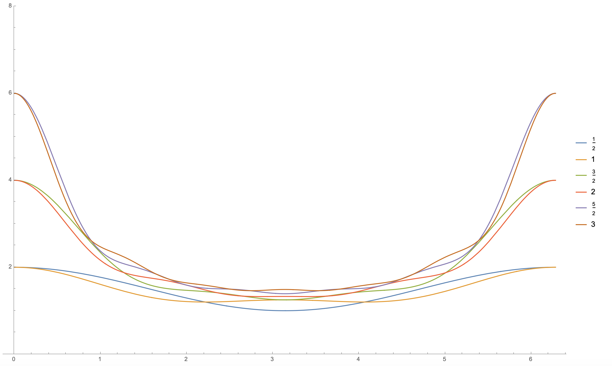
Refer to caption
Figure 14: When θ1=θ2\theta_{1}=\theta_{2}, the entanglement (80) for various spin valuesℓ\ell plotted in terms of the total angle α=θ1+θ2∈[0,2​π]\alpha=\theta_{1}+\theta_{2}\,\in[0,2\pi].

Recalling that the deficit angle given by δ=2​π−θ1−θ2=2​π−α\delta=2\pi-\theta_{1}-\theta_{2}=2\pi-\alpha at the cone summit provides a measure of the bulk curvature in fig.11(a), we can interpret the optimal angle confugirations in terms of discrete bulk geometry. The two maximal points correspond to dramatically different bulk geometries. Indeed, the angular-configuration θ1=θ2=0\theta_{1}=\theta_{2}=0 has a maximal deficit angle; it corresponds to the spin configurations j1,j2≪k1,k2j_{1},j_{2}\ll k_{1},k_{2} and k1≈k2k_{1}\approx k_{2}, with extremely elongated triangles, creating an extremely spiky bulk with maximal bulk curvature. On the other hand, the angle configuration θ1=θ2=π\theta_{1}=\theta_{2}=\pi has a vanishing deficit angle; it corresponds to spin configuratiosn j1≈k1+k2≈j2j_{1}\approx k_{1}+k_{2}\approx j_{2}, with flatten triangles and flat bulk geometry.

The β=π\beta=\pi branch lead to a minimal entanglement, with a vanishing leading order in t2t^{2}, S⁡(ρc​a​nAθ,t)=𝒪⁡(tOPEN4)CLOSES(\rho^{\theta}_{can_{A}},t)={\cal O}(t^{4)}. It corresponds to the maximal difference between the two triangle angles θ1\theta_{1} and θ2\theta_{2}.Geometrically, this corresponds to unbalanced configuration, with j1≪j2j_{1}\ll j_{2} or j2≪j1j_{2}\ll j_{1}, with one flatten triangle and one elongated triangle.

Now that we have looked into the small holonomy operator spin ℓ≪{ji,ki}\ell\ll\{j_{i},k_{i}\}, let us investigate the large spin regime, ℓ∼{ji,ki}\ell\sim\{j_{i},k_{i}\}. Since all the spins are assumed of the same order of magnitude, one can use the Ponzano-Regge asymptotic formula in terms of the Regge action for a tetrahedronosti_4824659; Roberts:1998zka; Rovelli:2014ssa:

{j1k1k2ℓK2K1}≈112​π​V​cos⁡(∑a​b(ja​b+12)​θa​b+π4)=12​−12​i​π​V​ei​S+12​12​i​π​V​e−i​S.\begin{Bmatrix}j_{1}&k_{1}&k_{2}\\ \ell&K_{2}&K_{1}\end{Bmatrix}\approx\frac{1}{\sqrt{12\pi V}}\cos\left(\sum_{ab}(j_{ab}+\frac{1}{2})\theta_{ab}+\frac{\pi}{4}\right)=\frac{1}{2\sqrt{-12{\rm{i}}\pi V}}e^{{\rm{i}}S}+\frac{1}{2\sqrt{12{\rm{i}}\pi V}}e^{-{\rm{i}}S}\,. (81)

The tetrahedron’s edge lengths are given by the spins ℓ,j1,k1,k2,K1,K2\ell,j_{1},k_{1},k_{2},K_{1},K_{2}. Its volume is VV and θa​b\theta_{ab} is the dihedral angle along the edge of length ja​bj_{ab}. The Regge action is given by S=∑a​b(ja​b+12)​θa​bS=\sum_{ab}(j_{ab}+\frac{1}{2})\theta_{ab}, which is understood to be the discretization of Einstein-Hilbert action (or more precisely of the Hartle-Hawking boundary term when the bulk curvature vanishes on-shell). This allows to rewrite (72) as:

ℓ∈ℕ+12:12​S​(ρc​a​nA,t)≈12​S​(ρc​a​nA(Regge),t)\displaystyle\ell\in{\mathbb{N}}+\frac{1}{2}:\qquad\frac{1}{2}S(\rho_{can_{A}},t)\approx\frac{1}{2}S(\rho^{(\textrm{Regge})}_{can_{A}},t) =\displaystyle= t2​(−1)φ​∑s=02​ℓcos⁡(SA​[s]−SB​[s])−sin⁡(SA​[s]+SB​[s])24​π​VA​[s]​VB​[s]​∏i=12(2​ki+1)\displaystyle t^{2}(-1)^{\varphi}\sum_{s=0}^{2\ell}\,\frac{\cos(S_{A}[s]-S_{B}[s])-\sin(S_{A}[s]+S_{B}[s])}{24\pi\sqrt{V_{A}[s]V_{B}[s]}}\prod_{i=1}^{2}(2k_{i}+1) (82)
+O⁡(t4),\displaystyle+O(t^{4})\,,
ℓ∈ℕ:12​S​(ρc​a​nA,t)≈12​S​(ρc​a​nA(Regge),t)\displaystyle\ell\in{\mathbb{N}}:\qquad\frac{1}{2}S(\rho_{can_{A}},t)\approx\frac{1}{2}S(\rho^{(\textrm{Regge})}_{can_{A}},t) =\displaystyle= t2​(−1)φ​∑s=02​ℓcos⁡(SA​[s]−SB​[s])−sin⁡(SA​[s]+SB​[s])24​π​VA​[s]​VB​[s]​∏i=12(2​ki+1)\displaystyle t^{2}(-1)^{\varphi}\sum_{s=0}^{2\ell}\,\frac{\cos(S_{A}[s]-S_{B}[s])-\sin(S_{A}[s]+S_{B}[s])}{24\pi\sqrt{V_{A}[s]V_{B}[s]}}\prod_{i=1}^{2}(2k_{i}+1) (83)
−t2[1−sin⁡(2​SA​[ℓ])]​[1−sin⁡(2​SB​[ℓ])]576​π2​VA​[ℓ]​VB​[ℓ]∏i=12(2ki+1)2+O(t4).\displaystyle-t^{2}\frac{[1-\sin(2S_{A}[\ell])][1-\sin(2S_{B}[\ell])]}{576\pi^{2}V_{A}[\ell]V_{B}[\ell]}\prod_{i=1}^{2}(2k_{i}+1)^{2}+O(t^{4})\,.

The Regge actions SA​[s]S_{A}[s] and SB​[s]S_{B}[s] corresponds respectively to the two tetrahedra dual to the vertices AA and BB, with edge lengths (ji,k1,k2,s,k2,k1)(j_{i},k_{1},k_{2},s,k_{2},k_{1}) respectivelk with i=1i=1 and i=2i=2. The phase φ=j1+j2+2​k1+2​k2\varphi=j_{1}+j_{2}+2k_{1}+2k_{2} and face amplitude factor (2​k1+1)​(2​k2+1)(2k_{1}+1)(2k_{2}+1) both depend on the bulk spins.

Let us conclude this section with a brief summary of our results on the example of the candy graph. The candy graph is the simplest graph with a non-trivial bulk. It is a special case of the 2-vertex graph Borja:2010gn; Borja:2010rc; Livine:2011up; Aranguren:2022nzn where the two vertices are linked by a couple of edges forming a loop in the bulk. This configuration allows to define non-trivial dynamical operators acting on the bulk geometry, for instance the loop holonomy operator, and to study the entanglement between the two bulk vertices generated by such dynamics.

In this context, we have explicitly computed the entanglement excitation created by the loop holoonomy operator acting on a pure spin network basis state at leading order in time, that is in t2t^{2}. We have considered and compared two measures of entanglement: the geometric entanglement studied in the the previous section and the bipartite entanglement entropy shared between the two vertices (given by the linear entropy of the reduced density matrix). We have shown that these two notions of entanglement match exactly a leading order, thus leading to a consistent picture of the entanglement excitation on the spin network state. Furthermore, in the semi-classical regime at large spins where spin networks can be provided with a discrete geometry interpretation in terms of dual triangulations, we have identified the initial configurations that optimize the excitation of entanglement by the loop operator as the (discrete) geometries with either maximal curvature or vanishing curvature.

V Triangle graph: multipartite entanglement

In this section, we wish to provide the reader with an example beyond the bipartite entanglement. We introduce the triangle graph, i.e. a triangle made with three vertices and with three boundary edges poking out from those vertices. The bulk triangle forms a loop on which we can act with the holonomy operator. This configuration allows to study both bipartite and tripartite entanglements by partionning the triplet of vertices, and to compare them with the geometric entanglement.

V.1 Bipartite entanglement on triangle graph

The triangle graph, as drawn on fig.15, is the direct extension of the candy graph to a bulk made of three vertices arranged around a single loop.

∙\bulletCCj3j_{3}∙\bulletAAj1j_{1}BBj2j_{2}k3k_{3}∙\bulletk1k_{1}∙\bulletk2k_{2}∙\bullet∙\bulletCCj3j_{3}∙\bulletAAj1j_{1}BBj2j_{2}j1j_{1}∑K1,K2,K3\displaystyle{\sum_{K_{1},K_{2},K_{3}}}K3K_{3}∙\bulletK1K_{1}∙\bulletK2K_{2}∙\bullet
Figure 15: The action of loop holonomy operator on triangle graph: it endows spin-superposition along the bulk edges.

The spin network Hilbert space on this triangle graph consists in the tensor product of three 3-valent intertwiner spaces, similarly to the candy graph,

ℋt​r​i=⨂v∈t​r​iℋv=ℋA⊗ℋB⊗ℋC,ℋA=⨁K2,K3InvSU⁡(2)​(𝒱j1⊗𝒱K2⊗𝒱K3),{\mathcal{H}}_{tri}=\bigotimes_{v\in tri}{\mathcal{H}}_{v}={\mathcal{H}}_{A}\otimes{\mathcal{H}}_{B}\otimes{\mathcal{H}}_{C}\,,\qquad{\mathcal{H}}_{A}=\bigoplus_{K_{2},K_{3}}\textrm{Inv}_{\mathrm{SU}(2)}\Big({\mathcal{V}}_{j_{1}}\otimes{\mathcal{V}}_{K_{2}}\otimes{\mathcal{V}}_{K_{3}}\Big)\,,

and similarly for ℋB{\mathcal{H}}_{B} and ℋC{\mathcal{H}}_{C}.

We wish to study the action of the loop holonomy operator on an arbitrary spin network basis state chosen as our initial state,

|Ψt​r​i,{ji,ki}⟩=|j1,k2,k3⟩A⊗|j2,k3,k1⟩B⊗|j3,k1,k2⟩C∈ℋA⊗ℋB⊗ℋC.\displaystyle|\Psi_{tri,\{j_{i},k_{i}\}}\rangle=|j_{1},k_{2},k_{3}\rangle_{A}\otimes|j_{2},k_{3},k_{1}\rangle_{B}\otimes|j_{3},k_{1},k_{2}\rangle_{C}\quad\in{\mathcal{H}}_{A}\otimes{\mathcal{H}}_{B}\otimes{\mathcal{H}}_{C}\,.

The loop holonomy operator affects the bulk spins {Ki}\{K_{i}\}, but not boundary spins {ji}\{j_{i}\},

χℓ^:\displaystyle\widehat{\chi_{\ell}}: InvSU⁡(2)​(𝒱j1⊗𝒱k2⊗𝒱k3)⊗InvSU⁡(2)​(𝒱j2⊗𝒱k3⊗𝒱k1)⊗InvSU⁡(2)​(𝒱j3⊗𝒱k1⊗𝒱k2)\displaystyle\textrm{Inv}_{\mathrm{SU}(2)}\Big({\mathcal{V}}_{j_{1}}\otimes{\mathcal{V}}_{k_{2}}\otimes{\mathcal{V}}_{k_{3}}\Big)\otimes\textrm{Inv}_{\mathrm{SU}(2)}\Big({\mathcal{V}}_{j_{2}}\otimes{\mathcal{V}}_{k_{3}}\otimes{\mathcal{V}}_{k_{1}}\Big)\otimes\textrm{Inv}_{\mathrm{SU}(2)}\Big({\mathcal{V}}_{j_{3}}\otimes{\mathcal{V}}_{k_{1}}\otimes{\mathcal{V}}_{k_{2}}\Big)
→⨁K1,K2,K3InvSU⁡(2)​(𝒱j1⊗𝒱K2⊗𝒱K3)⊗InvSU⁡(2)​(𝒱j2⊗𝒱K3⊗𝒱K1)⊗InvSU⁡(2)​(𝒱j3⊗𝒱K1⊗𝒱K2).\displaystyle\to\bigoplus_{K_{1},K_{2},K_{3}}\textrm{Inv}_{\mathrm{SU}(2)}\Big({\mathcal{V}}_{j_{1}}\otimes{\mathcal{V}}_{K_{2}}\otimes{\mathcal{V}}_{K_{3}}\Big)\otimes\textrm{Inv}_{\mathrm{SU}(2)}\Big({\mathcal{V}}_{j_{2}}\otimes{\mathcal{V}}_{K_{3}}\otimes{\mathcal{V}}_{K_{1}}\Big)\otimes\textrm{Inv}_{\mathrm{SU}(2)}\Big({\mathcal{V}}_{j_{3}}\otimes{\mathcal{V}}_{K_{1}}\otimes{\mathcal{V}}_{K_{2}}\Big)\,.

Following the same logic as with the candy graph, we compute the evolution of the state, truncated to leading order and properly normalized,

|Ψt​r​i,{ji,ki}​(ℓ,t)⟩=|Ψ​(t​r​i){ji,ki}⟩−i​t​∑{Ki}[Z​(t​r​i)ℓ{ji}]{ki}{Ki}​|Ψ​(t​r​i){ji,Ki}⟩1+t2​∑s=02​ℓ[Z​(t​r​i)s{ji}]{ki}{ki}.|\Psi_{tri,\{j_{i},k_{i}\}}(\ell,t)\rangle=\frac{|\Psi(tri)_{\{j_{i},k_{i}\}}\rangle-{\rm{i}}t\,\sum_{\{K_{i}\}}\,[Z(tri)_{\ell}^{\{j_{i}\}}]^{\{K_{i}\}}_{\phantom{\{K_{i}\}}\{k_{i}\}}\,|\Psi(tri)_{\{j_{i},K_{i}\}}\rangle}{\sqrt{1+t^{2}\sum_{s=0}^{2\ell}\,[Z(tri)_{s}^{\{j_{i}\}}]^{\{k_{i}\}}_{\phantom{\{k_{i}\}}\{k_{i}\}}}}\,. (84)

The transition matrix ZZ is expressed in terms of 6​j6j-symbols according to the general formula (18) for the action of the loop operator χℓ^\widehat{\chi_{\ell}},

[Z​(t​r​i)ℓ{ji}]{ki}{Ki}=(−1)∑i=13(ji+ki+Ki+ℓ)​{j1k2k3ℓK3K2}​{j2k3k1ℓK1K3}​{j3k1k2ℓK2K1}​∏i=13(2​ki+1)​(2​Ki+1).[Z(tri)_{\ell}^{\{j_{i}\}}]^{\{K_{i}\}}_{\phantom{\{K_{i}\}}\{k_{i}\}}=(-1)^{\sum_{i=1}^{3}(j_{i}+k_{i}+K_{i}+\ell)}\begin{Bmatrix}j_{1}&k_{2}&k_{3}\\ \ell&K_{3}&K_{2}\end{Bmatrix}\begin{Bmatrix}j_{2}&k_{3}&k_{1}\\ \ell&K_{1}&K_{3}\end{Bmatrix}\begin{Bmatrix}j_{3}&k_{1}&k_{2}\\ \ell&K_{2}&K_{1}\end{Bmatrix}\,\prod_{i=1}^{3}\sqrt{(2k_{i}+1)(2K_{i}+1)}\,. (85)

The normalization factor can then be evaluated to

Nt​r​i,{ji,ki}​(ℓ,t)\displaystyle N_{tri,\{j_{i},k_{i}\}}(\ell,t) =\displaystyle= 1+t2​∑s=02​ℓ(−1)j1+j2+j3+2​k1+2​k2+2​k3+3​s​{j1k2k3sk3k2}​{j2k3k1sk1k3}​{j3k1k2sk2k1}​∏i=13(2​ki+1)\displaystyle 1+t^{2}\sum_{s=0}^{2\ell}(-1)^{j_{1}+j_{2}+j_{3}+2k_{1}+2k_{2}+2k_{3}+3s}\begin{Bmatrix}j_{1}&k_{2}&k_{3}\\ s&k_{3}&k_{2}\end{Bmatrix}\begin{Bmatrix}j_{2}&k_{3}&k_{1}\\ s&k_{1}&k_{3}\end{Bmatrix}\begin{Bmatrix}j_{3}&k_{1}&k_{2}\\ s&k_{2}&k_{1}\end{Bmatrix}\prod_{i=1}^{3}(2k_{i}+1) (86)
=\displaystyle= 1+t2​∑K1,K2,K3{j1k2k3ℓK3K2}2​{j2k3k1ℓK1K3}2​{j3k1k2ℓK2K1}2​∏i=13(2​ki+1)​(2​Ki+1).\displaystyle 1+t^{2}\sum_{K_{1},K_{2},K_{3}}\begin{Bmatrix}j_{1}&k_{2}&k_{3}\\ \ell&K_{3}&K_{2}\end{Bmatrix}^{2}\begin{Bmatrix}j_{2}&k_{3}&k_{1}\\ \ell&K_{1}&K_{3}\end{Bmatrix}^{2}\begin{Bmatrix}j_{3}&k_{1}&k_{2}\\ \ell&K_{2}&K_{1}\end{Bmatrix}^{2}\prod_{i=1}^{3}(2k_{i}+1)(2K_{i}+1)\,. (87)

As for candy graph, this normalization factor is to be interpreted as the density of spin network basis states after the action of loop holonomy operator.

The initial spin network state is a basis state, thus is fully separable with vanishing entanglement. The final state is given by the following density matrix:

ρt​r​iA​B​C​(t)=|Ψt​r​i,{ji,ki}​(ℓ,t)⟩​⟨Ψc​a​n,{ji,ki}​(ℓ,t)|∈End​(ℋA⊗ℋB⊗ℋC)\displaystyle\rho_{tri_{ABC}}(t)=|\Psi_{tri,\{j_{i},k_{i}\}}(\ell,t)\rangle\langle\Psi_{can,\{j_{i},k_{i}\}}(\ell,t)|\quad\in\textrm{End}({\mathcal{H}}_{A}\otimes{\mathcal{H}}_{B}\otimes{\mathcal{H}}_{C}) (88)
=\displaystyle= 11+t2​∑s=02​ℓ[Z​(t​r​i)s{ji}]{ki}{ki}(|j1,k2,k3⟩⟨j1,k2,k3|A⊗|j2,k3,k1⟩⟨j2,k3,k1|B⊗|j3,k1,k2⟩⟨j3,k1,k2|C\displaystyle\frac{1}{1+t^{2}\sum_{s=0}^{2\ell}[Z(tri)_{s}^{\{j_{i}\}}]^{\{k_{i}\}}_{\phantom{\{k_{i}\}}\{k_{i}\}}}\bigg(|j_{1},k_{2},k_{3}\rangle\langle j_{1},k_{2},k_{3}|_{A}\otimes|j_{2},k_{3},k_{1}\rangle\langle j_{2},k_{3},k_{1}|_{B}\otimes|j_{3},k_{1},k_{2}\rangle\langle j_{3},k_{1},k_{2}|_{C}
+t2∑{Ki,Ki′}[Z(tri)ℓ{ji}]{ki}{Ki}[Z(tri)ℓ{ji}]{ki}{Ki′}|j1,K2,K3⟩⟨j1,K2′,K3′|A⊗|j2,K3,K1⟩⟨j2,K3′,K1′|B\displaystyle+t^{2}\sum_{\{K_{i},K^{\prime}_{i}\}}[Z(tri)_{\ell}^{\{j_{i}\}}]^{\{K_{i}\}}_{\phantom{\{K_{i}\}}\{k_{i}\}}[Z(tri)_{\ell}^{\{j_{i}\}}]^{\{K^{\prime}_{i}\}}_{\phantom{\{K^{\prime}_{i}\}}\{k_{i}\}}|j_{1},K_{2},K_{3}\rangle\langle j_{1},K^{\prime}_{2},K^{\prime}_{3}|_{A}\otimes|j_{2},K_{3},K_{1}\rangle\langle j_{2},K^{\prime}_{3},K^{\prime}_{1}|_{B}
⊗|j3,K1,K2⟩⟨j3,K1′,K2′|C\displaystyle\otimes|j_{3},K_{1},K_{2}\rangle\langle j_{3},K^{\prime}_{1},K^{\prime}_{2}|_{C}
−it∑{Ki}[Z(tri)ℓ{ji}]{ki}{Ki}|j1,K2,K3⟩⟨j1,k2,k3|A⊗|j2,K3,K1⟩⟨j2,k3,k1|B⊗|j3,K1,K2⟩⟨j3,k1,k2|C\displaystyle-{\rm{i}}t\sum_{\{K_{i}\}}[Z(tri)_{\ell}^{\{j_{i}\}}]^{\{K_{i}\}}_{\phantom{\{K_{i}\}}\{k_{i}\}}|j_{1},K_{2},K_{3}\rangle\langle j_{1},k_{2},k_{3}|_{A}\otimes|j_{2},K_{3},K_{1}\rangle\langle j_{2},k_{3},k_{1}|_{B}\otimes|j_{3},K_{1},K_{2}\rangle\langle j_{3},k_{1},k_{2}|_{C}
+it∑{Ki}[Z(tri)ℓ{ji}]{ki}{Ki}|j1,k2,k3⟩⟨j1,K2,K3|A⊗|j2,k3,k1⟩⟨j2,K3,K1|B⊗|j3,k1,k2⟩⟨j3,K1,K2|C).\displaystyle+{\rm{i}}t\sum_{\{K_{i}\}}[Z(tri)_{\ell}^{\{j_{i}\}}]^{\{K_{i}\}}_{\phantom{\{K_{i}\}}\{k_{i}\}}|j_{1},k_{2},k_{3}\rangle\langle j_{1},K_{2},K_{3}|_{A}\otimes|j_{2},k_{3},k_{1}\rangle\langle j_{2},K_{3},K_{1}|_{B}\otimes|j_{3},k_{1},k_{2}\rangle\langle j_{3},K_{1},K_{2}|_{C}\bigg)\,.

Now there are three possible bipartition of the triple tensor product ℋA⊗ℋB⊗ℋC{\mathcal{H}}_{A}\otimes{\mathcal{H}}_{B}\otimes{\mathcal{H}}_{C}. For the sake of convenience, let us look at the reduced density matrices for ℋA{\mathcal{H}}_{A}, ℋB{\mathcal{H}}_{B} and ℋC{\mathcal{H}}_{C} respectively, moreover, we only need to write down ρt​r​iA​(t)\rho_{tri_{A}}(t) and the other two cases are similar. Via tracing over ℋB​C{\mathcal{H}}_{BC}, the reduced density matrix is read

ρt​r​iA​(t)=TrB​C​ρt​r​iA​B​C​(t)\displaystyle\rho_{tri_{A}}(t)={\mathrm{Tr}}_{BC}\rho_{tri_{ABC}}(t) =\displaystyle= 11+t2​∑s=02​ℓ[Z​(t​r​i)s{ji}]{ki}{Ki}(|j1,k2,k3⟩⟨j1,k2,k3|A\displaystyle\frac{1}{1+t^{2}\sum_{s=0}^{2\ell}[Z(tri)_{s}^{\{j_{i}\}}]^{\{K_{i}\}}_{\phantom{\{K_{i}\}}\{k_{i}\}}}\bigg(|j_{1},k_{2},k_{3}\rangle\langle j_{1},k_{2},k_{3}|_{A} (89)
+t2∑K1,K2,K3([Z(tri)ℓ{ji}]{ki}K1​K2​K3)2|j1,K2,K3⟩⟨j1,K2,K3|A)∈End(ℋA).\displaystyle+t^{2}\sum_{K_{1},K_{2},K_{3}}\Big([Z(tri)_{\ell}^{\{j_{i}\}}]^{K_{1}K_{2}K_{3}}_{\phantom{K_{1}K_{2}K_{3}}\{k_{i}\}}\Big)^{2}|j_{1},K_{2},K_{3}\rangle\langle j_{1},K_{2},K_{3}|_{A}\bigg)\quad\in\textrm{End}({\mathcal{H}}_{A})\,.

This is a diagonal matrix with respect to basis |j1,K2,K3⟩∈ℋA|j_{1},K_{2},K_{3}\rangle\in{\mathcal{H}}_{A}, thus the eigenvalues of ρt​r​iA​(t)\rho_{tri_{A}}(t) can be directly read off from the expression above:

λρt​r​iA​[K2,K3]=δk2K2​δk3K3+t2​∑K1=|k1−ℓ|k1+ℓ{j1k2k3ℓK3K2}2​{j2k3k1ℓK1K3}2​{j3k1k2ℓK2K1}2​∏i=13(2​Ki+1)​(2​ki+1)1+t2​∑s=02​ℓ(−1)∑i=13(ji+ki+Ki+s)​{j1k2k3sk3k2}​{j2k3k1sk1k3}​{j3k1k2sk2k1}​∏i=13(2​ki+1).\lambda_{\rho_{tri_{A}}}[K_{2},K_{3}]=\frac{\delta^{K_{2}}_{k_{2}}\,\delta^{K_{3}}_{k_{3}}+t^{2}\sum_{K_{1}=|k_{1}-\ell|}^{k_{1}+\ell}\begin{Bmatrix}j_{1}&k_{2}&k_{3}\\ \ell&K_{3}&K_{2}\end{Bmatrix}^{2}\begin{Bmatrix}j_{2}&k_{3}&k_{1}\\ \ell&K_{1}&K_{3}\end{Bmatrix}^{2}\begin{Bmatrix}j_{3}&k_{1}&k_{2}\\ \ell&K_{2}&K_{1}\end{Bmatrix}^{2}\,\prod_{i=1}^{3}(2K_{i}+1)(2k_{i}+1)}{1+t^{2}\sum_{s=0}^{2\ell}(-1)^{\sum_{i=1}^{3}(j_{i}+k_{i}+K_{i}+s)}\begin{Bmatrix}j_{1}&k_{2}&k_{3}\\ s&k_{3}&k_{2}\end{Bmatrix}\begin{Bmatrix}j_{2}&k_{3}&k_{1}\\ s&k_{1}&k_{3}\end{Bmatrix}\begin{Bmatrix}j_{3}&k_{1}&k_{2}\\ s&k_{2}&k_{1}\end{Bmatrix}\,\prod_{i=1}^{3}(2k_{i}+1)}\,. (90)

The eigenvalues are labeled by the two spins K2K_{2} and K3K_{3}. This gives us the bipartite entanglement entropy of ℋA|ℋB⊗ℋC{\mathcal{H}}_{A}|{\mathcal{H}}_{B}\otimes{\mathcal{H}}_{C} up to second order in tt:

12​S​(ρt​r​iA)=12​(1−∑K2,K3λρt​r​iA​[K2,K3]2)\displaystyle\frac{1}{2}S(\rho_{tri_{A}})={{\frac{1}{2}\left(1-\sum_{K_{2},K_{3}}\lambda_{\rho_{tri_{A}}}[K_{2},K_{3}]^{2}\right)}} (91)
=\displaystyle= t2​(∑s=02​ℓ(−1)j1+j2+j3+2​k1+2​k2+2​k3+3​s​{j1k2k3sk3k2}​{j2k3k1sk1k3}​{j3k1k2sk2k1}​∏i=13(2​ki+1)CLOSE\displaystyle t^{2}\bigg(\sum_{s=0}^{2\ell}(-1)^{j_{1}+j_{2}+j_{3}+2k_{1}+2k_{2}+2k_{3}+3s}\begin{Bmatrix}j_{1}&k_{2}&k_{3}\\ s&k_{3}&k_{2}\end{Bmatrix}\begin{Bmatrix}j_{2}&k_{3}&k_{1}\\ s&k_{1}&k_{3}\end{Bmatrix}\begin{Bmatrix}j_{3}&k_{1}&k_{2}\\ s&k_{2}&k_{1}\end{Bmatrix}\prod_{i=1}^{3}(2k_{i}+1)
−∑K1=|k1−ℓ|k1+ℓ{j1k2k3ℓk3k2}2{j2k3k1ℓK1k3}2{j3k1k2ℓk2K1}2(2K1+1)(2k1+1)(2k2+1)2(2k3+1)2)+O(t4).\displaystyle-\sum_{K_{1}=|k_{1}-\ell|}^{k_{1}+\ell}\begin{Bmatrix}j_{1}&k_{2}&k_{3}\\ \ell&k_{3}&k_{2}\end{Bmatrix}^{2}\begin{Bmatrix}j_{2}&k_{3}&k_{1}\\ \ell&K_{1}&k_{3}\end{Bmatrix}^{2}\begin{Bmatrix}j_{3}&k_{1}&k_{2}\\ \ell&k_{2}&K_{1}\end{Bmatrix}^{2}\,(2K_{1}+1)(2k_{1}+1)(2k_{2}+1)^{2}(2k_{3}+1)^{2}\bigg)+O(t^{4})\,.

As for the candy graph, no 1st-order of tt appears at all and the leading order is directly in t2t^{2}.

One gets the linear entropies for the vertices BB and CC by a straightforward cyclic permutation of the labels. Generally, the three bipartite entanglement entropies have different values due to the a priori different values of the initial spins. Nonetheless, when ℓ∈ℕ+12\ell\in{\mathbb{N}}+\frac{1}{2}, all three bipartite entanglement entropies are equal to each other at the leading order in t2t^{2}. We trace this back to the triangle condition on the {6​j}\{6j\}-symbols, which eliminates the second term in the entropy formula above. Hence we conclude

Result V.1.

For an odd holonomy spin ℓ∈N+12\ell\in N+\frac{1}{2}, the bipartite entanglement entropies on triangle graph satisfy S⁡(ρt​r​iA)=S⁡(ρt​r​iB)=S⁡(ρt​r​iC)S(\rho_{tri_{A}})=S(\rho_{tri_{B}})=S(\rho_{tri_{C}}) at leading order in t2t^{2}. This common leading order term is given

12​S​(ρt​r​iA)∼t2​(∑s=02​ℓ(−1)j1+j2+j3+2​k1+2​k2+2​k3+3​s​{j1k2k3sk3k2}​{j2k3k1sk1k3}​{j3k1k2sk2k1}​∏i=13(2​ki+1)).{{\frac{1}{2}}}S(\rho_{tri_{A}})\sim t^{2}\bigg(\sum_{s=0}^{2\ell}(-1)^{j_{1}+j_{2}+j_{3}+2k_{1}+2k_{2}+2k_{3}+3s}\begin{Bmatrix}j_{1}&k_{2}&k_{3}\\ s&k_{3}&k_{2}\end{Bmatrix}\begin{Bmatrix}j_{2}&k_{3}&k_{1}\\ s&k_{1}&k_{3}\end{Bmatrix}\begin{Bmatrix}j_{3}&k_{1}&k_{2}\\ s&k_{2}&k_{1}\end{Bmatrix}\prod_{i=1}^{3}(2k_{i}+1)\bigg)\,. (92)

Those triangle inequalities further implies that that S⁡(ρt​r​iA)=S⁡(ρt​r​iB)=S⁡(ρt​r​iC)S(\rho_{tri_{A}})=S(\rho_{tri_{B}})=S(\rho_{tri_{C}}) reach the same plateau value when the holonomy operator spin is larger than its critical value, ℓ>min⁡{2​k1,2​k2,2​k3}\ell>\min\{2k_{1},2k_{2},2k_{3}\}, no matter whenever ℓ\ell is odd or even.

We now compare the bipartite entanglement to the tripartite entanglement, defined as the geometric entanglement.

V.2 Tripartite entanglement

In order to quantify the multipartite entanglement on the triangle graph, we use the geometric entanglement. We can compute the geometric measure of entanglement as explained previously: the geometric entanglement is given by the maximal projection of the evolving state onto the spin network basis, which is, at very early times tt, its projection onto the initial spin network basis state, that is by the contribution K1,2,3=k1,2,3K_{1,2,3}=k_{1,2,3}:

λmax=|⟨Ψt​r​i,{ji,ki}​(ℓ,0)|Ψt​r​i,{ji,ki}​(ℓ,t)⟩|2=1+t2​([Z​(t​r​i)ℓ{ji}]{ki}{ki})21+t2​∑s=02​ℓ[Z​(t​r​i)s{ji}]{ki}{ki}.\lambda_{\max}=\big|\langle\Psi_{tri,\{j_{i},k_{i}\}}(\ell,0)|\Psi_{tri,\{j_{i},k_{i}\}}(\ell,t)\rangle\big|^{2}=\frac{1+t^{2}\Big([Z(tri)_{\ell}^{\{j_{i}\}}]^{\{k_{i}\}}_{\phantom{\{K_{i}\}}\{k_{i}\}}\Big)^{2}}{1+t^{2}\sum_{s=0}^{2\ell}\,[Z(tri)_{s}^{\{j_{i}\}}]^{\{k_{i}\}}_{\phantom{\{k_{i}\}}\{k_{i}\}}}\,. (93)

Hence it leads to the geometric measure of entanglement on triangle graph:

Sg​[Ψt​r​i,{ji,ki}​(ℓ,t)]\displaystyle S_{g}[\Psi_{tri,\{j_{i},k_{i}\}}(\ell,t)] =\displaystyle= t2​∏i=13(2​ki+1)​∑s=02​ℓ(−1)∑i=13(ji+2​ki+s)​{j1k2k3sk3k2}​{j2k3k1sk1k3}​{j3k1k2sk2k1}\displaystyle t^{2}\prod_{i=1}^{3}(2k_{i}+1)\sum_{s=0}^{2\ell}\,(-1)^{\sum_{i=1}^{3}(j_{i}+2k_{i}+s)}\begin{Bmatrix}j_{1}&k_{2}&k_{3}\\ s&k_{3}&k_{2}\end{Bmatrix}\begin{Bmatrix}j_{2}&k_{3}&k_{1}\\ s&k_{1}&k_{3}\end{Bmatrix}\begin{Bmatrix}j_{3}&k_{1}&k_{2}\\ s&k_{2}&k_{1}\end{Bmatrix} (94)
−t2∏i=13(2ki+1)2{j1k2k3ℓk3k2}2{j2k3k1ℓk1k3}2{j3k1k2ℓk2k1}2+O(t4).\displaystyle-t^{2}\prod_{i=1}^{3}(2k_{i}+1)^{2}\begin{Bmatrix}j_{1}&k_{2}&k_{3}\\ \ell&k_{3}&k_{2}\end{Bmatrix}^{2}\begin{Bmatrix}j_{2}&k_{3}&k_{1}\\ \ell&k_{1}&k_{3}\end{Bmatrix}^{2}\begin{Bmatrix}j_{3}&k_{1}&k_{2}\\ \ell&k_{2}&k_{1}\end{Bmatrix}^{2}+O(t^{4})\,.

This is a straightforward extension of the formula (72) derived for the candy graph, where we’ve added the relevant {6​j}\{6j\}-symbols. As earlier, the geometric entanglement excitation reaches a plateau, due to the triangle inequalities on the spins, when the holonomy operator spin grows beyond a critical value, ℓ>min⁡{2​k1,2​k2,2​k3}\ell>\min\{2k_{1},2k_{2},2k_{3}\}. Moreover, when the spin is odd, ℓ∈ℕ+12\ell\in{\mathbb{N}}+\frac{1}{2}, the second term in (94) vanishes, as for the bipartite entanglement in last subsection.

The plots 16 compare the bipartite entanglement entropies and geometric entanglement:

  • •

    (i) they are equal when the holonomy spin is odd, ℓ∈ℕ+12\ell\in{\mathbb{N}}+\frac{1}{2};

  • •

    (ii) for small spins ℓ\ell, those measures of entanglement are clearly distinct, but they tend to converge as the spin ℓ\ell increases, and they are eventually constant and equal beyond the critical value ℓ>min⁡{2​k1,2​k2,2​k3}\ell>\min\{2k_{1},2k_{2},2k_{3}\}.

Refer to caption
(a) Spins j1=3,j2=4,j3=5,k1=6,k2=8,k3=7j_{1}=3,j_{2}=4,j_{3}=5,k_{1}=6,k_{2}=8,k_{3}=7.
Refer to caption
(b) Spins j1=5/2,j2=7/2,j3=4,k1=6,k2=8,k3=11/2j_{1}=5/2,j_{2}=7/2,j_{3}=4,k_{1}=6,k_{2}=8,k_{3}=11/2.
Refer to caption
(c) Spins j1=6,j2=9,j3=7,k1=12,k2=11,k3=10j_{1}=6,j_{2}=9,j_{3}=7,k_{1}=12,k_{2}=11,k_{3}=10.
Refer to caption
(d) Spins j1=9/2,j2=11/2,j3=7,k1=12,k2=16,k3=27/2j_{1}=9/2,j_{2}=11/2,j_{3}=7,k_{1}=12,k_{2}=16,k_{3}=27/2.
Figure 16: The comparison between bipartite entanglement entropies and geometric measure of entanglement, where blue point is for 12​SA\frac{1}{2}S_{A}, orange point for 12​SB\frac{1}{2}S_{B}, green point for 12​SC\frac{1}{2}S_{C} and red point for SgS_{g}.

One could also have computed the geometric entanglement by gauge-fixing and working out the closure defect’s probability distribution. Since the bulk graph consists in a single loop made of three edges, there are three ways to gauge-fix: choosing k1k_{1} as the “loopy spin”, i.e. the edge which is not gauge-fixed and gauge-fixing the edges associated with k2k_{2} and k3k_{3}, plus the two other possibilities of choosing k2k_{2} or k3k_{3} as the “loopy spin”.

For instance, contracting the edges carrying k2k_{2} and k3k_{3} and keeping k1k_{1}, we obtain the probability distribution of the closure defect as

pk1​(J)=(2​J+1)​(2​k2+1)​(2​k3+1)​∑L(2​L+1)​{j3j2Lk1k1Jk2k3j1}2,p_{k_{1}}(J)=(2J+1)(2k_{2}+1)(2k_{3}+1)\sum_{L}(2L+1)\begin{Bmatrix}j_{3}&j_{2}&L\\ k_{1}&k_{1}&J\\ k_{2}&k_{3}&j_{1}\end{Bmatrix}^{2}\,, (95)

with the normalization ∑Jpk1​(J)=1\sum_{J}p_{k_{1}}(J)=1. This probability distribution gives the 2nd-order time derivative of geometric entanglement:

12​d2​Sgd​t2|t=0\displaystyle\frac{1}{2}\frac{\mathrm{d}^{2}S_{g}}{\mathrm{d}t^{2}}\Big|_{t=0} =\displaystyle= ∑J,L(2​J+1)​(2​L+1)​(2​k1+1)​(2​k2+1)​(2​k3+1)​{j3j2Lk1k1Jk2k3j1}2​∑s=02​ℓ(−1)J+s+2​k1​{Jk1k1sk1k1}\displaystyle\sum_{J,L}(2J+1)(2L+1)(2k_{1}+1)(2k_{2}+1)(2k_{3}+1)\begin{Bmatrix}j_{3}&j_{2}&L\\ k_{1}&k_{1}&J\\ k_{2}&k_{3}&j_{1}\end{Bmatrix}^{2}\sum_{s=0}^{2\ell}(-1)^{J+s+2k_{1}}\begin{Bmatrix}J&k_{1}&k_{1}\\ s&k_{1}&k_{1}\end{Bmatrix} (96)
−(∑J,L(2​J+1)​(2​L+1)​(2​k1+1)​(2​k2+1)​(2​k3+1)​{j3j2Lk1k1Jk2k3j1}2​(−1)J+ℓ+2​k1​{Jk1k1sk1k1})2.\displaystyle-\left(\sum_{J,L}(2J+1)(2L+1)(2k_{1}+1)(2k_{2}+1)(2k_{3}+1)\begin{Bmatrix}j_{3}&j_{2}&L\\ k_{1}&k_{1}&J\\ k_{2}&k_{3}&j_{1}\end{Bmatrix}^{2}(-1)^{J+\ell+2k_{1}}\begin{Bmatrix}J&k_{1}&k_{1}\\ s&k_{1}&k_{1}\end{Bmatrix}\right)^{2}\,.

It is straightforward to check that these results does not actually depend on the choice of gauge-fixing and that it gives the same expression for the leading order entanglement computed above in eqn.(94). This can be shown by using the Biedenharn-Elliott identity. More precisely, we need to prove the following relation:

{j1k2k3ℓk3k2}​{j2k3k1ℓk1k3}​{j3k1k2ℓk2k1}\displaystyle\begin{Bmatrix}j_{1}&k_{2}&k_{3}\\ \ell&k_{3}&k_{2}\end{Bmatrix}\begin{Bmatrix}j_{2}&k_{3}&k_{1}\\ \ell&k_{1}&k_{3}\end{Bmatrix}\begin{Bmatrix}j_{3}&k_{1}&k_{2}\\ \ell&k_{2}&k_{1}\end{Bmatrix} (97)
=\displaystyle= (−1)∑i=13(ji+2​ki+ℓ)​∑J,L(2​J+1)​(2​L+1)​{j3j2Lk1k1Jk2k3j1}2​(−1)J+ℓ+2​k1​{Jk1k1ℓk1k1}.\displaystyle(-1)^{\sum_{i=1}^{3}(j_{i}+2k_{i}+\ell)}\sum_{J,L}(2J+1)(2L+1)\begin{Bmatrix}j_{3}&j_{2}&L\\ k_{1}&k_{1}&J\\ k_{2}&k_{3}&j_{1}\end{Bmatrix}^{2}(-1)^{J+\ell+2k_{1}}\begin{Bmatrix}J&k_{1}&k_{1}\\ \ell&k_{1}&k_{1}\end{Bmatrix}\,.

Starting from the left side, we use the Biedenharn-Elliot identity twice: we first recouple the first two 6​j6j-symbols via the Biedenharn-Elliot identity, which results in three 6​j6j-symbols, then we take one of them and recouple it to the third 6​j6j-symbol of the original prooductone via the Biedenharn-Elliot identity again. This gives:

{ℓk3k3j1k2k2}​{ℓk1k1j2k3k3}​{ℓk2k2j3k1k1}\displaystyle\begin{Bmatrix}\ell&k_{3}&k_{3}\\ j_{1}&k_{2}&k_{2}\end{Bmatrix}\begin{Bmatrix}\ell&k_{1}&k_{1}\\ j_{2}&k_{3}&k_{3}\end{Bmatrix}\begin{Bmatrix}\ell&k_{2}&k_{2}\\ j_{3}&k_{1}&k_{1}\end{Bmatrix} (98)
=\displaystyle= ∑L′,J(−1)j1+j2+j3+2​k1+2​k2+2​k3+ℓ​(−1)J+ℓ+2​k1​{k1k1Jk1k1ℓ}​(2​J+1)​(2​L′+1)​{j1j2L′k1k2k3}2​{Jj3L′k2k1k1}2,\displaystyle\sum_{L^{\prime},J}(-1)^{j_{1}+j_{2}+j_{3}+2k_{1}+2k_{2}+2k_{3}+\ell}(-1)^{J+\ell+2k_{1}}\begin{Bmatrix}k_{1}&k_{1}&J\\ k_{1}&k_{1}&\ell\end{Bmatrix}(2J+1)(2L^{\prime}+1)\begin{Bmatrix}j_{1}&j_{2}&L^{\prime}\\ k_{1}&k_{2}&k_{3}\end{Bmatrix}^{2}\begin{Bmatrix}J&j_{3}&L^{\prime}\\ k_{2}&k_{1}&k_{1}\end{Bmatrix}^{2}\,,

Finally, we deal with the two squared 6​j6j-symbols by the contraction formula of Racah coefficients (see brink1968angular, page 143)

(−1)2​h+2​d​∑c(2​c+1)​{aikfbc}​{abcdefghi}={aikhdg}​{bfkdhe},(-1)^{2h+2d}\sum_{c}(2c+1)\begin{Bmatrix}a&i&k\\ f&b&c\end{Bmatrix}\begin{Bmatrix}a&b&c\\ d&e&f\\ g&h&i\end{Bmatrix}=\begin{Bmatrix}a&i&k\\ h&d&g\end{Bmatrix}\begin{Bmatrix}b&f&k\\ d&h&e\end{Bmatrix}\,, (99)

which allows to write

∑L′(2​L+1)​{j1j2L′k1k2k3}2​{Jj3L′k2k1k1}2\displaystyle\sum_{L^{\prime}}(2L+1)\begin{Bmatrix}j_{1}&j_{2}&L^{\prime}\\ k_{1}&k_{2}&k_{3}\end{Bmatrix}^{2}\begin{Bmatrix}J&j_{3}&L^{\prime}\\ k_{2}&k_{1}&k_{1}\end{Bmatrix}^{2} (100)
=\displaystyle= ∑L,L′′(2​L+1)​(2​L′′+1)​{j1j2L′j3JL}​{j1j2L′j3JL′′}​{j1JLk2k1j3k3k1j2}​{j1JL′′k2k1j3k3k1j2}={j1JLk2k1j3k3k1j2}2,\displaystyle\sum_{L,L^{\prime\prime}}(2L+1)(2L^{\prime\prime}+1)\begin{Bmatrix}j_{1}&j_{2}&L^{\prime}\\ j_{3}&J&L\end{Bmatrix}\begin{Bmatrix}j_{1}&j_{2}&L^{\prime}\\ j_{3}&J&L^{\prime\prime}\end{Bmatrix}\begin{Bmatrix}j_{1}&J&L\\ k_{2}&k_{1}&j_{3}\\ k_{3}&k_{1}&j_{2}\end{Bmatrix}\begin{Bmatrix}j_{1}&J&L^{\prime\prime}\\ k_{2}&k_{1}&j_{3}\\ k_{3}&k_{1}&j_{2}\end{Bmatrix}=\begin{Bmatrix}j_{1}&J&L\\ k_{2}&k_{1}&j_{3}\\ k_{3}&k_{1}&j_{2}\end{Bmatrix}^{2}\,,

By symmetry of 9​j9j-symbol, this proves the wanted eqn.(97).

Finally, we can look at the semi-classical regime at large spins {ji,ki}\{j_{i},k_{i}\}, in which the spin network has a clear interpretation in terms of dual triangulation: the triangle graph is dual to a open tetrahedron to which one has removed one triangle, as drawn on fig.18. This missing triangle corresponds to the the boundary edge of the graph, decorated with the spins (j1,j2,j3)(j_{1},j_{2},j_{3}). For large spins, assuming that ℓ≪{ji,ki}\ell\ll\{j_{i},k_{i}\}, one can apply Racah’s approximation (77) for 6​j6j-symbols to the geometric entanglement formula (94) and write it in terms of Legendre polynomials in the cosine of the triangle angles, as illustrated on figure 17:

Sg​[Ψt​r​i,{ji,ki}​(ℓ,t)]∼t2​∑s=02​ℓPs​(cos⁡θ1)​Ps​(cos⁡θ2)​Ps​(cos⁡θ3)−t2​[Ps​(cos⁡θ1)​Ps​(cos⁡θ2)​Ps​(cos⁡θ3)]2+O⁡(t4)S_{g}[\Psi_{tri,\{j_{i},k_{i}\}}(\ell,t)]\sim t^{2}\sum_{s=0}^{2\ell}P_{s}(\cos\theta_{1})P_{s}(\cos\theta_{2})P_{s}(\cos\theta_{3})-t^{2}[P_{s}(\cos\theta_{1})P_{s}(\cos\theta_{2})P_{s}(\cos\theta_{3})]^{2}+O(t^{4}) (101)

with the convention that half-integer Legendre polynomials Pℓ​(x)P_{\ell}(x) vanish, for ℓ∈ℕ+12\ell\in{\mathbb{N}}+\frac{1}{2}. The angles are given in terms of the spins by

cos⁡θ1=k2​(k2+1)+k3​(k3+1)−j1​(j1+1)2​k2​(k2+1)​k3​(k3+1),\displaystyle\cos\theta_{1}=\frac{k_{2}(k_{2}+1)+k_{3}(k_{3}+1)-j_{1}(j_{1}+1)}{2\sqrt{k_{2}(k_{2}+1)k_{3}(k_{3}+1)}}\,, (102)
cos⁡θ2=k3​(k3+1)+k1​(k1+1)−j2​(j2+1)2​k3​(k3+1)​k1​(k1+1),\displaystyle\cos\theta_{2}=\frac{k_{3}(k_{3}+1)+k_{1}(k_{1}+1)-j_{2}(j_{2}+1)}{2\sqrt{k_{3}(k_{3}+1)k_{1}(k_{1}+1)}}\,,
cos⁡θ3=k1​(k1+1)+k2​(k2+1)−j3​(j3+1)2​k1​(k1+1)​k2​(k2+1).\displaystyle\cos\theta_{3}=\frac{k_{1}(k_{1}+1)+k_{2}(k_{2}+1)-j_{3}(j_{3}+1)}{2\sqrt{k_{1}(k_{1}+1)k_{2}(k_{2}+1)}}\,.

This expression allows us to study how the entanglement varies with respect to the spin network initial data.

∙\bulletj3j_{3}∙\bulletj1j_{1}j2j_{2}∙\bullet∙\bullet∙\bulletk1k_{1}k2k_{2}k3k_{3}∙\bulletθ3\theta_{3}θ1\theta_{1}θ2\theta_{2}
Figure 17: The dual triangulation (brown lines) on triangle graph. The angles are given by (102).

As for the bipartite system defined on the candy graph, the extremal configurations for the entanglement excitation by the holonomy operator are given by extremal geometries: spiky tetrahedral geometries with flatten triangles and maximal curvature. More precisely, to start with, vanishing angles θ1=θ2=θ3=0\theta_{1}=\theta_{2}=\theta_{3}=0 maximizes the multipartite entanglement excitation, as for the candy graph geometry. It corresponds to the asymptotic limit of spiky tetrahedron, as drawn on fig.18, where the summit is sent to infinity, which is interpreted as an extremal bulk curvature. Similarly, angular configurations θ1=0,θ2=θ3=π\theta_{1}=0,\theta_{2}=\theta_{3}=\pi, and its two other permutations, also produce a maximal entanglement growth. In terms of spins and thus of edge lengths, this corresponds to j1≪k2,k3j_{1}\ll k_{2},k_{3}, j2≈k1+k3j_{2}\approx k_{1}+k_{3}, j3≈k1+k2j_{3}\approx k_{1}+k_{2}, which satisfy the triangular inequalities for (j1,j2,j3)(j_{1},j_{2},j_{3}).

On the contrary, the angle configurations θ1=θ2=0,θ3=π\theta_{1}=\theta_{2}=0,\theta_{3}=\pi and its other two permutations, as well as θ1=θ2=θ3=π\theta_{1}=\theta_{2}=\theta_{3}=\pi, all lead to a minimal entanglement, i.e. vanishing entanglement excitation at leading order in t2t^{2}. Translating in terms of spins and edge lengths, the former case corresponds to j1,j2≪k1,k2,k3j_{1},j_{2}\ll k_{1},k_{2},k_{3}, j3≈k1+k2j_{3}\approx k_{1}+k_{2}, which doesn’t satisfy the triangular inequalities for (j1,j2,j3)(j_{1},j_{2},j_{3}), and thus is not an allowed spin network configuration. The latter case, with equal angles θ1=θ2=θ3=π\theta_{1}=\theta_{2}=\theta_{3}=\pi , corresponds to j1≈k2+k3j_{1}\approx k_{2}+k_{3}, j2≈k3+k1j_{2}\approx k_{3}+k_{1}, j3≈k1+k2j_{3}\approx k_{1}+k_{2}, which is allowed by the triangular inequalities.

k3k_{3}k2k_{2}k1k_{1}j1j_{1}j3j_{3}j2j_{2}∙\bullet∙\bullet∙\bullet∙\bullet
Figure 18: A spike triangulation.

To conclude this section, we extended to the triangular graph our analysis of the entanglement excitation by the loop holonomy operator on a spin network basis state. This has confirmed our general analysis of the geometric entanglement for an arbitrary graph. More precisely, we have computed analytically and numerically both the linear entanglement entropies for bipartitions of the graph and the geometric entanglement and checked that they match at leading order in the time tt. Since the initial state is unentangled, the evolution starts with a vanishing entanglement then grows in t2t^{2}. Moreover, we have identified the spin network configurations with extremal entanglement excitations, which unsurprisingly correspond to discrete geometries with extremal curvature. This is a positive step towards establishing a more thorough and precise dictionary between quantum entanglement, quantum geometry and its dynamics in the framework of loop quantum gravity.

VI Conclusion & Outlook

The present paper is dedicated to the study of entanglement in loop quantum gravity. More precisely, we looked into the evolution of entanglement under the action of the holonomy operator. Intuitively, the holonomy operator acting on a loop of a spin network state will act at once on all the intertwiners living at the nodes on the loop and will entangle them. More precisely, we studied the unitary evolution generated by a holonomy operator on an initial state given by a spin network basis state. Such an initial state has fixed spins and intertwiners, it is thus a separable state carrying absolutely no entanglement. The evolution will naturally create entanglement between the vertices of the spin network and our goal was to compute the excitation of entanglement by the holonomy operator. The holonomy around a loop representing a discretized measure of curvature, this leads to a relation between excitations of the geometry -“quanta of curvature”- and excitations of the information -multipartite entanglement- over spin network basis states. This fits in the larger program of interpreting and reconstructing the quantum geometry of space-time from quantum information concepts.

At the technical level, we introduced a notion of geometric entanglement to measure the multipartite entanglement carried by a spin network state, defined as the distance between that state and the set of separable states, identified (up to minor subtleties) to the set of spin network basis states. This is understood as witness of how much the intertwiners of a spin network, i.e. its quanta of volume, are entangled with each other. Starting from an initial spin network basis state, thus with vanishing entanglement, we find that the first order time derivative at initial time always vanishes, so that the leading order behavior is a quadratic growth of the entanglement. We show that the second order derivative is simply given by the dispersion of the holonomy operator, which can in turn be computed from the probability distribution of the “closure defect” around the loop (i.e. the total spin recoupling the spins of all the edges attached to the loop). Considering holonomy operators with arbitrary spin ℓ∈ℕ/2\ell\in{\mathbb{N}}/2, we find that this entanglement excitation grows with the spin ℓ\ell and exhibits a plateau behavior: the entanglement excitation saturates and reaches its maximal value when the spin ℓ\ell becomes larger than all the spins around the loop.

We illustrate this analysis through its application to the simplest spin networks with non-trivial bulk and boundary: the candy graph, consisting in two vertices linked by a single loop, and the triangle graph, consisting in three vertices linked by a single loop, both with arbitrary number of boundary edges poking out of the bulk vertices. These configurations allow to study explicitly the correlation and entanglement between the intertwiners living at the graph vertices. We compute the geometric entanglement and express it in terms of 6j-symbols from spin recoupling, which allows to study its low-spin and large-spin regimes. We further compute the bipartite entanglement created by the holonomy operator, defined as the entropy of the reduced density matrix, and show that it fits exactly at leading order with the notion of geometric entanglement we introduced.

Since holonomy operators are the basic building blocks of the Hamiltonian dynamics of loop quantum gravity, this work gives a first hint of the effect of the dynamics on the quantum information carried by spin network states. We hope that further characterizing the various operators of loop quantum gravity through their effect on the correlation and entanglement between intertwiners will allow to reformulate the whole dynamics and notion of physical states entirely in quantum information terms.

Acknowledgement

Q.C. is financially supported by the China Scholarship Council.

Appendix A Examples of entanglement evolution

A.1 Time-dependent Bell state

Let |Ψ⁡(t)⟩=cos⁡t⁡|00⟩+sin⁡t⁡|11⟩|\Psi(t)\rangle=\cos t|00\rangle+\sin t|11\rangle. The Hermitian operator in the case has matrix representation H^=(0−ii0)\widehat{H}=\begin{pmatrix}0&-{\rm{i}}\\ {\rm{i}}&0\end{pmatrix} with respect to basis {|00⟩,|11⟩}\{|00\rangle,|11\rangle\}. This bipartite state initiates with the unentangled state |00⟩|00\rangle. Within t∈[0,π/4)t\in[0,\pi/4), the |Φ⁡(t)⟩|\Phi(t)\rangle is chosen as |00⟩|00\rangle, while within t∈(π/4,3​π/4)t\in(\pi/4,3\pi/4), the |Φ⁡(t)⟩|\Phi(t)\rangle is chosen as |11⟩|11\rangle. At the instant t=π/4t=\pi/4, there is ambiguity to define the unique |Φ⁡(t)⟩|\Phi(t)\rangle. Also, the |Φ⁡(t)⟩|\Phi(t)\rangle is discontinuous at t=π/4t=\pi/4. However, the maximal projection |⟨Φ⁡(t)|Ψ⁡(t)⟩|2|\langle\Phi(t)|\Psi(t)\rangle|^{2} is still differentiable along t→s+t\to s+ and t→s−t\to s- (the left and right derivative could be different).

A.2 Black hole evaporation toy model

We give another simple example whose maximal projection |⟨Φ⁡(t)|Ψ⁡(t)⟩|2|\langle\Phi(t)|\Psi(t)\rangle|^{2} is also differentiable. Consider the Hamiltonian H^=i⁡(a†​b†−a​b)\widehat{H}={\rm{i}}(a^{\dagger}b^{\dagger}-ab) acting on the unentangled initial state |0⟩A⊗|0⟩B|0\rangle_{A}\otimes|0\rangle_{B}. The evolution produces the entangled quantum state:

|Ψ⁡(t)⟩=1cosh⁡t​∑n=0∞tanhn⁡t​|n⟩A⊗|n⟩B.|\Psi(t)\rangle=\frac{1}{\cosh t}\sum_{n=0}^{\infty}\tanh^{n}t|n\rangle_{A}\otimes|n\rangle_{B}\,. (103)

The Schmidt eigenvalues are labelled by an interger nn and read λn=tanh2​n⁡t/cosh2⁡t\lambda_{n}=\tanh^{2n}t/\cosh^{2}t. The bipartite entanglement entropy as a function of the time tt is given by:

S⁡(t)=ln⁡cosh2⁡t−sinh2⁡t​ln⁡tanh2⁡t,withlimt→0d​S​(t)d​t=0,limt→0d2​S​(t)d​t2→∞.S(t)=\ln\cosh^{2}t-\sinh^{2}t\ln\tanh^{2}t\,,\qquad\textrm{with}\quad\lim_{t\to 0}\frac{\mathrm{d}S(t)}{\mathrm{d}t}=0\,,\quad\lim_{t\to 0}\frac{\mathrm{d}^{2}S(t)}{\mathrm{d}t^{2}}\to\infty\,. (104)

This entropy evolution function grows asymptotically linearly as 2​t2t. However, the maximal Schmidt eigenvalue is always given by the 0-mode, for the number of quanta n=0n=0, since |tanh2⁡t|<1|\tanh^{2}t|<1, so that the separable projection is constant, |Φ⁡(t)⟩=|0⟩A⊗|0⟩B|\Phi(t)\rangle=|0\rangle_{A}\otimes|0\rangle_{B} for all times tt. Then the maximal Schmidt eigenvalue λmax​(t)=λ0=1/cosh2⁡t\lambda_{\max}(t)=\lambda_{0}=1/\cosh^{2}t is smooth and gives the geometric measure of entanglement.

References

  • (1) M. Gaul and C. Rovelli, “Loop quantum gravity and the meaning of diffeomorphism invariance,” Lect. Notes Phys. 541 (2000) 277–324, arXiv:gr-qc/9910079.
  • (2) T. Thiemann, “Modern canonical quantum general relativity,” arXiv:gr-qc/0110034.
  • (3) C. Rovelli and F. Vidotto, Covariant Loop Quantum Gravity: An Elementary Introduction to Quantum Gravity and Spinfoam Theory. Cambridge Monographs on Mathematical Physics. Cambridge University Press, 11, 2014.
  • (4) N. Bodendorfer, “An elementary introduction to loop quantum gravity,” arXiv:1607.05129.
  • (5) C. Rovelli and L. Smolin, “Discreteness of area and volume in quantum gravity,” Nucl. Phys. B 442 (1995) 593–622, arXiv:gr-qc/9411005. [Erratum: Nucl.Phys.B 456, 753–754 (1995)].
  • (6) A. Ashtekar and J. Lewandowski, “Quantum theory of geometry. 1: Area operators,” Class. Quant. Grav. 14 (1997) A55–A82, arXiv:gr-qc/9602046.
  • (7) A. Ashtekar and J. Lewandowski, “Quantum theory of geometry. 2. Volume operators,” Adv. Theor. Math. Phys. 1 (1998) 388–429, arXiv:gr-qc/9711031.
  • (8) T. Thiemann, “Quantum spin dynamics (QSD),” Class. Quant. Grav. 15 (1998) 839–873, arXiv:gr-qc/9606089.
  • (9) T. Thiemann, “Quantum spin dynamics (qsd). 2.,” Class. Quant. Grav. 15 (1998) 875–905, arXiv:gr-qc/9606090.
  • (10) M. P. Reisenberger and C. Rovelli, “’Sum over surfaces’ form of loop quantum gravity,” Phys. Rev. D 56 (1997) 3490–3508, arXiv:gr-qc/9612035.
  • (11) J. C. Baez, “Spin foam models,” Class. Quant. Grav. 15 (1998) 1827–1858, arXiv:gr-qc/9709052.
  • (12) J. W. Barrett and L. Crane, “Relativistic spin networks and quantum gravity,” J. Math. Phys. 39 (1998) 3296–3302, arXiv:gr-qc/9709028.
  • (13) L. Freidel and K. Krasnov, “Spin foam models and the classical action principle,” Adv. Theor. Math. Phys. 2 (1999) 1183–1247, arXiv:hep-th/9807092.
  • (14) E. R. Livine, The Spinfoam Framework for Quantum Gravity. PhD thesis, Lyon, IPN, 2010. arXiv:1101.5061.
  • (15) M. Dupuis, Spin Foam Models for Quantum Gravity and semi-classical limit. PhD thesis, Lyon, Ecole Normale Superieure, 2010. arXiv:1104.2765.
  • (16) A. Perez, “The Spin Foam Approach to Quantum Gravity,” Living Rev. Rel. 16 (2013) 3, arXiv:1205.2019.
  • (17) R. De Pietri, L. Freidel, K. Krasnov, and C. Rovelli, “Barrett-Crane model from a Boulatov-Ooguri field theory over a homogeneous space,” Nucl. Phys. B 574 (2000) 785–806, arXiv:hep-th/9907154.
  • (18) M. P. Reisenberger and C. Rovelli, “Space-time as a Feynman diagram: The Connection formulation,” Class. Quant. Grav. 18 (2001) 121–140, arXiv:gr-qc/0002095.
  • (19) L. Freidel, “Group field theory: An Overview,” Int. J. Theor. Phys. 44 (2005) 1769–1783, arXiv:hep-th/0505016.
  • (20) D. Oriti, “The Group field theory approach to quantum gravity,” arXiv:gr-qc/0607032.
  • (21) S. Carrozza, Tensorial methods and renormalization in Group Field Theories. PhD thesis, Orsay, LPT, 2013. arXiv:1310.3736.
  • (22) D. Oriti, J. P. Ryan, and J. Thürigen, “Group field theories for all loop quantum gravity,” New J. Phys. 17 (2015), no. 2, 023042, arXiv:1409.3150.
  • (23) W. Donnelly and L. Freidel, “Local subsystems in gauge theory and gravity,” JHEP 09 (2016) 102, arXiv:1601.04744.
  • (24) A. Feller and E. R. Livine, “Entanglement entropy and correlations in loop quantum gravity,” Class. Quant. Grav. 35 (2018), no. 4, 045009, arXiv:1710.04473.
  • (25) E. R. Livine and D. R. Terno, “Quantum black holes: Entropy and entanglement on the horizon,” Nucl. Phys. B741 (2006) 131–161, arXiv:gr-qc/0508085.
  • (26) E. R. Livine and D. R. Terno, “Bulk Entropy in Loop Quantum Gravity,” Nucl. Phys. B794 (2008) 138–153, arXiv:0706.0985.
  • (27) W. Donnelly, “Entanglement entropy in loop quantum gravity,” Phys. Rev. D77 (2008) 104006, arXiv:0802.0880.
  • (28) E. R. Livine and D. R. Terno, “The Entropic boundary law in BF theory,” Nucl. Phys. B 806 (2009) 715–734, arXiv:0805.2536.
  • (29) W. Donnelly, “Decomposition of entanglement entropy in lattice gauge theory,” Phys. Rev. D85 (2012) 085004, arXiv:1109.0036.
  • (30) W. Donnelly, “Entanglement entropy and nonabelian gauge symmetry,” Class. Quant. Grav. 31 (2014), no. 21, 214003, arXiv:1406.7304.
  • (31) A. Feller and E. R. Livine, “Ising Spin Network States for Loop Quantum Gravity: a Toy Model for Phase Transitions,” Class. Quant. Grav. 33 (2016), no. 6, 065005, arXiv:1509.05297.
  • (32) E. Bianchi, L. Hackl, and N. Yokomizo, “Entanglement entropy of squeezed vacua on a lattice,” Phys. Rev. D92 (2015), no. 8, 085045, arXiv:1507.01567.
  • (33) A. Feller and E. R. Livine, “Surface state decoherence in loop quantum gravity, a first toy model,” Class. Quant. Grav. 34 (2017), no. 4, 045004, arXiv:1607.00182.
  • (34) E. Bianchi, J. Guglielmon, L. Hackl, and N. Yokomizo, “Loop expansion and the bosonic representation of loop quantum gravity,” Phys. Rev. D 94 (2016), no. 8, 086009, arXiv:1609.02219.
  • (35) C. Delcamp, B. Dittrich, and A. Riello, “On entanglement entropy in non-Abelian lattice gauge theory and 3D quantum gravity,” JHEP 11 (2016) 102, arXiv:1609.04806.
  • (36) E. R. Livine, “Intertwiner Entanglement on Spin Networks,” Phys. Rev. D97 (2018), no. 2, 026009, arXiv:1709.08511.
  • (37) B. Baytas, E. Bianchi, and N. Yokomizo, “Gluing polyhedra with entanglement in loop quantum gravity,” Phys. Rev. D98 (2018), no. 2, 026001, arXiv:1805.05856.
  • (38) F. Anzà and G. Chirco, “Typicality in spin-network states of quantum geometry,” Phys. Rev. D94 (2016), no. 8, 084047, arXiv:1605.04946.
  • (39) G. Chirco, F. M. Mele, D. Oriti, and P. Vitale, “Fisher Metric, Geometric Entanglement and Spin Networks,” Phys. Rev. D 97 (2018), no. 4, 046015, arXiv:1703.05231.
  • (40) E. Colafranceschi, G. Chirco, and D. Oriti, “Holographic maps from quantum gravity states as tensor networks,” Phys. Rev. D 105 (2022), no. 6, 066005, arXiv:2105.06454.
  • (41) G. Chirco, E. Colafranceschi, and D. Oriti, “Bulk area law for boundary entanglement in spin network states: Entropy corrections and horizon-like regions from volume correlations,” Phys. Rev. D 105 (2022), no. 4, 046018, arXiv:2110.15166.
  • (42) E. Colafranceschi and G. Adesso, “Holographic entanglement in spin network states: a focused review,” arXiv:2202.05116.
  • (43) T.-C. Wei and P. M. Goldbart, “Geometric measure of entanglement and applications to bipartite and multipartite quantum states,” Phys. Rev. A 68 (Oct, 2003) 042307.
  • (44) L. Amico, R. Fazio, A. Osterloh, and V. Vedral, “Entanglement in many-body systems,” Rev. Mod. Phys. 80 (2008) 517–576, arXiv:quant-ph/0703044.
  • (45) O. Gühne and G. Tóth, “Entanglement detection,” Physics Reports 474 (2009), no. 1, 1–75.
  • (46) A. Ashtekar and E. Bianchi, “A short review of loop quantum gravity,” Rept. Prog. Phys. 84 (2021), no. 4, 042001, arXiv:2104.04394.
  • (47) Q. Chen and E. R. Livine, “Loop quantum gravity’s boundary maps,” Class. Quant. Grav. 38 (2021), no. 15, 155019, arXiv:2103.08409.
  • (48) F. Anzà and G. Chirco, “Fate of the Hoop Conjecture in Quantum Gravity,” Phys. Rev. Lett. 119 (2017), no. 23, 231301, arXiv:1703.05241.
  • (49) V. Bonzom, E. R. Livine, and S. Speziale, “Recurrence relations for spin foam vertices,” Class. Quant. Grav. 27 (2010) 125002, arXiv:0911.2204.
  • (50) E. F. Borja, J. Diaz-Polo, I. Garay, and E. R. Livine, “Dynamics for a 2-vertex Quantum Gravity Model,” Class. Quant. Grav. 27 (2010) 235010, arXiv:1006.2451.
  • (51) G. Ponzano and T. Regge, “Semiclassical limits of Racah coefficients,” pp 1-58 of Spectroscopic and Group Theoretical Methods in Physics. Block, F. (ed.). New York, John Wiley and Sons, Inc., 1968.
  • (52) J. Roberts, “Classical 6j-symbols and the tetrahedron,” Geom. Topol. 3 (1999), no. 1, 21–66, arXiv:math-ph/9812013.
  • (53) E. F. Borja, L. Freidel, I. Garay, and E. R. Livine, “U(N) tools for Loop Quantum Gravity: The Return of the Spinor,” Class. Quant. Grav. 28 (2011) 055005, arXiv:1010.5451.
  • (54) E. R. Livine and M. Martin-Benito, “Classical Setting and Effective Dynamics for Spinfoam Cosmology,” Class. Quant. Grav. 30 (2013) 035006, arXiv:1111.2867.
  • (55) E. Aranguren, I. n. Garay, and E. R. Livine, “Classical dynamics for Loop Gravity: The 2-vertex model,” arXiv:2204.00307.
  • (56) D. Brink and G. Satchler, Angular Momentum. Oxford library of the physical sciences. Clarendon P., 1968.