Implicit Motion-Compensated Network for Unsupervised Video Object Segmentation
Abstract
Unsupervised video object segmentation (UVOS) aims at automatically separating the primary foreground object(s) from the background in a video sequence. Existing UVOS methods either lack robustness when there are visually similar surroundings (appearance-based) or suffer from deterioration in the quality of their predictions because of dynamic background and inaccurate flow (flow-based). To overcome the limitations, we propose an implicit motion-compensated network (IMCNet) combining complementary cues (i.e., appearance and motion) with aligned motion information from the adjacent frames to the current frame at the feature level without estimating optical flows. The proposed IMCNet consists of an affinity computing module (ACM), an attention propagation module (APM), and a motion compensation module (MCM). The light-weight ACM extracts commonality between neighboring input frames based on appearance features. The APM then transmits global correlation in a top-down manner. Through coarse-to-fine iterative inspiring, the APM will refine object regions from multiple resolutions so as to efficiently avoid losing details. Finally, the MCM aligns motion information from temporally adjacent frames to the current frame which achieves implicit motion compensation at the feature level. We perform extensive experiments on and YouTube-Objects. Our network achieves favorable performance while running at a faster speed compared to the state-of-the-art methods. Our code is available at https://github.com/xilin1991/IMCNet.
Index Terms:
Video processing, video object segmentation, attention mechanism, motion compensation.I Introduction

The goal of unsupervised video object segmentation (UVOS) is to identify and segment the most visually prominent object(s) from the background in videos. The UVOS has attracted significant attention owing to its widespread applications in content-based video retrieval [1], video matting [2], video editing [3], video analysis [4], and video compression [5, 6, 7, 8, 9, 10]. Different from the semi-supervised [11, 12, 13, 14] and weakly-supervised [15, 16] video object segmentation, which has a full mask of the object(s) of interest in the first frame of a video sequence, the UVOS is more challenging because of the lack of user interactions.
Primary object candidates that span through the whole video sequence are provided by the algorithm on the UVOS. This primary foreground object(s) should capture human attention when the whole video sequence is watched, i.e., objects that are more likely to be followed by the human gaze. Inspired by a biological mechanism known as human attention [17], the UVOS system should have remarkable motion perception capabilities to quickly orient gaze to moving objects in dynamic scenes. We argue that the primary object(s) in a video should be (i) the most distinguishable in a single frame, (ii) repeatedly appearing throughout the video sequence, and (iii) moving objects in the video. The former represents the intra-frame discriminability (local dependence), and the latter two are inter-frame consistency (global dependence). Fully exploiting these three properties is crucial for determining the primary video object(s).
For example, methods in [18, 19, 20] can work well for discovering saliency objects in static images. However, they may not be applicable for UVOS tasks due to motions, occlusion, and distractor objects, as shown in Fig. 1 (d). Therefore, it is necessary to make use of inter-frame consistency (global dependence) to make up for the drawbacks caused by ignoring temporal correlation. Earlier traditional methods [21, 22, 23] have been investigated from these perspectives, it is inadequately considered by current deep learning-based solutions. The deep learning-based methods [24, 25, 26] and reinforcement learning-based methods [27, 28] boost the performance of UVOS systems, and yet still face challenges considering local variations and global consistency (uniformity), meanwhile. These works mainly proceed in two directions. One line [25, 29, 24, 30, 31, 32, 33, 34] is with a learned model of multi-modality inputs. They typically used optical flows as an additional modality to capture motion cues, which leverage the global temporal motion information cross frames. In general, these multi-modality-based methods introduce an additional pre-processing stage to predict the optical flow. However, due to the accuracy of optical flow prediction, the quality of the UVOS model could deteriorate over time. The noise introduced by the optical flow may misguide the UVOS models to predict the primary object(s) incorrectly as shown in Fig. 1 (a), (f). Another limitation of those methods is that they ignore local discriminability, such as texture features. The other direction is based on single-modality [26, 35, 36, 37, 38, 39, 40, 41, 42, 43], which matches the appearance of inter-frame to exploit long-term correlations from a global perspective. However, they incur significant computational costs on the condition that non-local operation conducts matrix multiplication operation. More importantly, due to only mining the matched pixels across the frames, previous appearance-based methods may be wrongly taken visually similar surroundings as the primary object(s) (Fig. 1 (b), (c), (e)).
In this paper, we propose an Implicit Motion-Compensated Network (IMCNet) for the UVOS. The IMCNet takes several frames from the same video as inputs to mine the long-term correlations and align temporally adjacent frames to the current frame for implicit motion compensation at the feature level. The proposed model consists of an affinity computing module (ACM), an attention propagation module (APM), and a motion compensation module (MCM). In our method, the two main objectives are achieved, mining local dependence and offsetting global dependence from adjacent frames. For mining local dependence, the light-weight ACM is designed, it is extended from a co-attention [44, 45] mechanism. Instead of computing affinity in the feature space, a novel key-value embedding module is used in ACM to largely reduce the computational cost and meet high performance. Through this process, we will see in the experimental results that the IMCNet is not only more robust but also more efficient than the algorithm in [37, 38, 39, 40, 41, 42, 43]. Then, the APM is applied to retain the primary object(s) at each level of the top-down decoder architecture. Through coarse-to-fine iterative inspiring, the APM will refine object regions from multiple resolutions so as to efficiently avoid losing details. Finally, the MCM is proposed to implicitly capture global dependence from adjacent frames. Unlike the previous optical flow-based UVOS methods [31, 33, 34], our approach can adaptively offset the current moment from neighboring frames at the feature level without explicit motion estimation. This is another advantage of our IMCNet.
Inspired by the deformable convolution [46, 47], our MCM uses features from the adjacent frames to dynamically predict offsets of sampling convolution kernels. These dynamic kernels are gradually applied to neighboring features, and offsets are propagated to the current frame to facilitate precise motion compensation, similar to the motion transition based on optical flow in multi-modality models [31, 33, 34, 48, 49]. Moreover, an additional temporal-spatial fusion is employed after the cascading deformable operation to further improve the robustness of compensation. A temporal attention by computing the similarity between the feature of compensation and the current frame is applied to utilize motion cues better. After fusing with temporal attention, a spatial attention operation is further introduced to automatically select relatively important features effectively in spatial channels. In addition, a joint training strategy is introduced for training our IMCNet to effectively learn the discriminative features of the primary object(s). It helps our model focus more on pixels of the primary object(s) with the guidance of the saliency information, thus filtering out the similar surrounding noise.
Our contributions in this paper are several folds:
- •
A novel Implicit Motion-Compensated Network (IMCNet) combining complementary cues (i.e., appearance and motion) is proposed to overcome the existing method’s drawback. This is achieved by a light-weight ACM, APM, and MCM. Extensive experiments on [50] and YouTube-Objects [51] show IMCNet achieves favorable performance while running at faster speed and using much fewer parameters compared to the state-of-the-arts.
- •
A light-weight ACM which embeds a co-attention mechanism with a novel key-value component is introduced to explore the consistent representation from a global perspective, while at the same time helping to capture appearance features within inter-frames.
- •
A novel MCM is incorporated for modeling motion information of salient objects within multiple input frames, leading to a more powerful moving object pattern recognition framework.
- •
A new joint training strategy is proposed to train our models on UVOS and SOD datasets, to enhance the representation ability of local discriminability.
II Proposed method
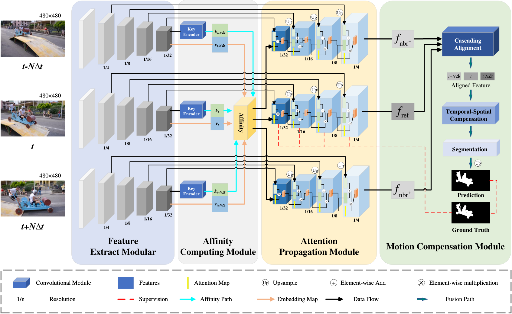
An end-to-end deep neural network, i.e., IMCNet, is proposed to mine the long-term correlations and implicitly encodes motion cues in feature level across multi-frames for the UVOS. The overall framework of the proposed IMCNet is shown in Fig. 2. The IMCNet is designed as an encoder-decoder fashion since this kind of architecture is able to preserve low-level details to refine high-level global contexts. The proposed model comprises four key modules: feature extract modular (FEM) (§II-A), ACM (§II-B), APM (§II-C), and MCM (§II-D). Given consecutive frames () with an interval of frames, the middle frame is selected as the center frame and the other frames are neighboring frames, and indicates the spatial resolution of images. The aim of our model is to estimate the corresponding objects masks .
II-A Feature extract modular
Our FEM relies on a parallel structure encoder to jointly embed adjacent frames, which has been proven effective in many time-related video tasks. The shared feature encoder, which is pre-trained using the ImageNet [52] and DUTS [53], takes several frames as inputs. We take the last four convolutional blocks of the ResNet [54] as the backbone for each stream. The FEM takes consecutive frames as inputs, including the center frame and neighboring frames, for exploring a consensus representation in a high-dimensional space. We denote the extracted embeddings of as , where indicates the -th () residual stage, is scales, and represents the feature map channels, respectively.
II-B Affinity computing module
To focus more on the primary object(s) in , we delve into the intra-frame features supported by neighboring frames. In detail, we build a key encoder module to extract independently a key feature for each frame and is symmetric in the center and neighboring frames11 1 Key encoder processing on features from FEM does not depend on whether they come from center or neighboring frames. The same key encoder encodes the center and neighboring frames into key maps instead of several independent key encoders.. The rationales are that 1) Global dependence is computationally efficient to extract from key features than the value (), and 2) Global dependence exists in key features without redundancy, and there is a lot of distraction on value features. The ACM then takes two-stream data (i.e. key and value features) of each moment as inputs to compute similarity.
Key encoder. We take features from the FEM as inputs of the key encoder. Both the center and the neighboring frames are first encoded into key maps through the residual block, where and is smaller than the input image () and is set as 64. It can be formally represented as:
| (1) |
where is typically composed of two convolutional layers followed by a ReLU activation as a projection head from the backbone feature to the key space ( dimensional).
Affinity computing. Similarities among key features of the center and neighboring frames are computed to determine when-and-where to retrieve relevant primary object(s) correlation from input frames. Key features are learned to represent the correlations among the center and neighboring frames in their feature embedding space. Value features store detailed information for producing the object mask prediction. As shown in Fig. 3, given consecutive embedding features from the same video, we first compute the affinity matrix among input frames:
| (2) |
where [] denotes the concatenation operation and is a trainable weight matrix. The affinity matrix can effectively capture global dependence between the feature space of input images. In order to keep consistency among the video frames, is approximately factorized into two invertible matrices and . Then, Eq. 2 can be rewritten as:
| (3) | ||||
where . This operation is equivalent to applying channel-wise feature transformations to key features before computing the similarity.
After obtaining the affinity matrix , as shown in the light blue area in Fig. 3, we normalize row-wise with a softmax function to derive an attention map conditioned on neighboring images and achieve enhanced features.
| (4) |
With the normalized affinity matrix , the attention summaries for the feature embedding for each frame can be computed as a weighted sum of the value feature with efficient matrix multiplication (see the green areas in Fig. 3):
| (5) |
which is then passed to the APM.
II-C Attention propagation module
In general, the FPN [55] decoder is built upon the bottom-up backbone, and the induced high-level features will be gradually diluted when transmitted to lower layers. To this end, we propose an APM to connect encoder-decoder pairs of our IMCNet, as shown in Fig. 4. The APM progressively refines the skip-connection of FEM via higher-level prediction and can locate primary object(s) more accurately without the interference of irrelevant surroundings. Specifically, for each layer, the skip-connection of FEM is guided by the higher-level prediction to produce the final feature . At the top of the APM, we take weighted by the enhanced feature as an immediate feature to predict the first guide map :
| (6) |
where , , and are element-wise multiplication, element-wise multiplication with broadcasting, and global average pooling operation. is implemented by two convolutional layers followed by a sigmoid layer. After that, the APM further fed the guide map into the next layer in a recursive manner:
| (7) |
where ‘’ is the element-wise multiplication. is the up-sampling operation with stride 2 via bilinear interpolation. is typically composed of a residual block, with 64 kernels. It is similar to lateral connections of FPN [55]. The feature maps are then enhanced with features from the bottom-up pathway via lateral connection, and then refine it to obtain . consists of a head convolutional layer and a residual block and reduces the refined features to 64 channels. As the last step in the APM, we adopt two convolutional layers followed by a sigmoid layer to predict the side masks for deep supervision. The side masks can effectively hold the attention on the primary object(s) in each layer, as presented in the ablation study of section III. The last is the final output into the MCM for learning motion information. , named as , represents the output of the APM, in which input center frame . denote and , respectively (i.e., is the moment after the center frame, and vice versa).
II-D Motion compensation module
The MCM is proposed to align the features from neighboring frames to the center frame’s feature space for implicit motion compensation. As illustrated in Fig. 2, our MCM includes three sub-modules: a cascading alignment, a temporal-spatial compensation, and a segmentation.
Cascading alignment. Taking advantage of the deformable convolution network (DCN) [46, 47], we use an adaptive deformable kernel to achieve feature-level alignment. Different from optical flow-based methods, the alignment is applied on feature of each frame, denoted by and . As such, image warping is not required. The alignment module consists of multiple alignment operations organized in a cascaded manner, as shown in Fig. 5. We first take the feature of the center moment as a reference feature to align each neighboring feature , and the feature-level offset between the reference feature and neighboring feature is estimated. In this process, the reference and neighboring feature are concatenated before the transformation with a typical convolution layer and a light-weight offset generator :
| (8) |
where denotes cascaded layer in depth, is the learnable parameters, and represents the concatenation operation. In addition, we have . For simplicity, we omit the superscript for , and then can be formulated as:
| (9) |
Here, refers to learnable offsets for the convolution kernels of sampling locations. For instance, the regular grid of convolution kernel has 9 sampling locations, where . Then, DCN is applied to align the neighboring features to the reference feature with the guidance of the offset map :
| (10) | ||||
where is aligned feature at the -th stage (). and denote the weight and sampling locations of a convolutional kernel. As the is fractional, the sampling operation is implemented by using bilinear interpolation as in [46].
Cascading alignment module consists of several regular and deformable convolutional layers. For the offset generation phase, it concatenates and () and then uses a convolution layer to reduce the channel number of the concatenated feature map and follow the same kernel size convolution layer to predict the sampling parameters. Finally, the aligned feature is obtained from and based on the DCN, where . We use a four-stage cascaded structure, i.e., , which gradually refines the coarsely aligned features. The cascading alignment module in such a coarse-to-fine manner improves the alignment at the feature level.
Temporal-spatial compensation. Inspired by the CBAM [56], we propose temporal-spatial compensation (TSC) to exploit both temporal and spatial-wise attention on each frame. We focus on ‘where’ is an informative part supported by reference feature . In addition, we employ a pyramid structure to increase the attention receptive field due to unequally information of different aligned induced by occlusion and blur.
Given the reference feature and concatenated feature as inputs, the TSC sequentially infers 2D temporal attention map and a spatial attention , where denotes concatenate operation. The overall fusion process can be summarized as:
| (11) |
where ‘’ denotes the element-wise multiplication, and is a light-weight encoder with two convolutional layers followed by a ReLU activation. The temporal attention is implemented by calculating the similarity distance:
| (12) |
where . and are achieved with simple convolution layers. and denote channel-wise summation and sigmoid activation function. The spatial attention employs a pyramid design to increase the attention receptive field, can be obtained by:
| (13) |
where and are the typical convolution layer with dimensional reductions as original input channels. and represent max and average pooling layers with stride 2. Note that we add embedding spatial attention to spatial enhanced features to enhance losing important information on the regions with attention values close to zero. is the final refined output. Fig. 6 depicts the computation process of each attention map.

Segmentation. The segmentation module consists of a residual block (with 64 filters) and a convolutional layer (with one filter and sigmoid) for the final segmentation prediction based on the last output of TSC.
II-E Joint training strategy
A possible issue of the existing methods is that the temporal consistency is not maintained across the whole of the video sequence in the presence of visual similar objects or surroundings. The reason is that these methods focus on mining the correlation (global dependence) between consecutive frames, but pay less attention to the saliency object (local dependence), leading to inaccurate segmentation results. To alleviate this problem, we use the SOD and UVOS datasets to jointly train our model for the UVOS task. The efficient joint training strategy is summarized in Fig. 7.

The SOD and UVOS datasets are divided into two groups: ImageSet and VideoSet. The ImageSet obtained by sampling from DUTS [53] dataset consists of each individual image, and the VideoSet is temporal related consecutive frames getting from the [50] dataset. images or video clips where one clip contains frames are randomly sampled in each mini-batch from DUTS or datasets, respectively. One mini-batch ImageSet is repeated after mini-batches VideoSet. The ratio is given by
| (14) |
where denotes the floor function, and is return the size of the dataset. The role of the ImageSet is that the saliency object constraint is enforced to make the problem tractable. Through the above steps, the IMCNet can effectively improve the final segmentation results, as presented in section III.
II-F Loss functions
The loss functions in [57] are adopted to jointly measure the prediction in the pixel level by binary cross-entropy loss [58], in the patch level by SSIM loss [59], as well as in the region level by IoU loss [60]:
| (15) |
where denotes the segmentation prediction and refers to the binary ground-truth.
Given consecutive frames from a video sequence, our IMCNet predicts a final segmentation mask and intermediate segmentation side-outputs through -th () level of APM, and our APM is deeply supervised with the last four stages, i.e. . The total loss is formulated as:
| (16) | ||||
III Experiments
Extensive experimental results are presented to evaluate the proposed IMCNet.
III-A Datasets and evaluation metrics
To test the performance of our method, we carry out comprehensive experiments on two UVOS datasets:
[50] is currently the most popular VOS benchmark, which consists of 50 high-quality video sequences (30 videos for training and 20 for testing). Each frame is densely annotated pixel-wise ground-truth for the foreground objects. We train our IMCNet on the training set and evaluate on the validation set. For quantitative evaluation, we adopt two standard metrics suggested by [50], namely region similarity , which is the intersection-over-union of the prediction and ground-truth, boundary accuracy , which measures the accuracy of the predicted mask boundaries. These measures can be averaged to give an overall score.
YouTube-Objects [51] contains 126 web video sequences that assign 10 semantic object categories with more than 20,000 frames in total. All the video sequences are used for performance evaluation. Following YouTube-Objects’s evaluation protocol, we use the region similarity to measure the segmentation performance.
III-B Implementation details
III-B1 Detailed network architecture
The backbone of IMCNet is the ResNet101 [54], for each input frame of size , the frame is a down-sample to the size of in the last four layers of ResNet101. The network takes three consecutive frames (i.e., ) with an interval of four frames (i.e., ) as inputs unless otherwise specified. The output size of our IMCNet is , for the UVOS task, we use the bilinear interpolate algorithm to restore the original size of the input. For the ACM, we implement weight matrices and in Eq. 3 using two convolutional layers with 64 kernels, respectively. The channel size in the TSC module is set to 64.
III-B2 Training settings
The training data consists of three parts: 1) all training data from the [50], including 30 videos with about 2K frames; 2) a subset of the training set of YouTube-VOS [61] selected 18K frames, which is obtained by sampling images containing a single object per sequence; 3) DUTS-TR which is the training set of DUTS [53] has more than 10K images. The training process is divided into two stages. Stage 1: we first pre-train our network for 200K iterations on a subset of YouTube-VOS. During this training period, the entire network is trained using Adam [62] optimizer ( and ) with a learning rate of for the FEM, for the ACM and APM decoder, and the MCM is set as . The batch size is set to , and the weight decay is . Stage 2: we fine-tune the entire network on the training set of and DUTS with our joint training strategy. In this stage, the Adam optimizer is used with an initial learning rate of , , and for each of the above-mention modules, respectively. We train our network for 155K iterations in the second training stage. Data augmentation (e.g., scaling, flipping, and rotation) is also adopted for both image and video data. Our IMCNet is implemented in PyTorch [63]. All experiments and analyses are conducted on an NVIDIA TITAN RTX GPU, and the overall training time is about 72 hours.
III-B3 Test settings
On the test time, we resize the input frame to , and feed three consecutive frames with an interval of four frames into the network for segmentation. The segmentation mask of the center frame is obtained from the IMCNet. We follow the common protocol used in existing works [39, 43] and employ multi-scale and mirrored inputs to enhance the final segmentation mask without CRFs and instance pruning.
III-B4 Runtime
During testing, the forward estimation of our IMCNet takes around 0.05s per frame, while the post-processing takes about 0.2s.
III-C Ablation study
To demonstrate the influence of each component in the IMCNet, we perform an ablation study on the test set of . The evaluation criterion is mean region similarity () and mean boundary accuracy ().
III-C1 Effectiveness of ACM
To demonstrate the effectiveness of the ACM, we gradually remove the affinity computing and the key encoder process in our model, denoted as w/o. ACM and w/o. key encoder, respectively. It means that the features in the last convolution stage of the FEM are directly fed into the APM to achieve segmentation results. The results can be referred in the sub-table named ACM in Table I. From the results, we can observe that the performance of the variant without ACM (affinity computing + key encoder) is lower than our full model (with affinity computing + key encoder) in terms of mean , and lower on mean , respectively. In other words, ACM is key to improving the performance of our proposed method ( and on mean and mean , respectively). On this basis, we only introduced the affinity computing process, the performance of the variant without the key encoder is improved by and in terms of mean and mean higher than the variant without ACM. This indicates that affinity computing improves the performance of the model ( and on mean and mean , respectively). After that, we can observe that the performance of our full model (with affinity computing and key encoder) is and higher than the variant without key encoder on mean and , respectively. This validates the effectiveness of our key encoder that eliminates the redundancy by only focusing on the features related to the primary object(s). Meanwhile, our model can address the UVOS task by capturing global dependence from the multi-frames, which verifies the effectiveness of ACM.
| Network Variant | val | |||
|---|---|---|---|---|
| Mean | Mean | |||
| ACM | ||||
| w/o. ACM | 80.0 | -2.7 | 78.0 | -3.1 |
| w/o. key encoder (only affinity computing) | 80.6 | -2.1 | 78.7 | -2.4 |
| APM | ||||
| w/o. APM | 80.4 | -2.3 | 80.1 | -1.0 |
| Cascading Alignment | ||||
| regular | 81.5 | -1.2 | 80.0 | -1.1 |
| 79.6 | -3.1 | 78.4 | -2.7 | |
| 80.7 | -2.0 | 79.3 | -1.8 | |
| 81.4 | -1.3 | 80.1 | -1.0 | |
| 82.7 | - | 81.1 | - | |
| 82.0 | -0.7 | 81.0 | -0.1 | |
| TSC | ||||
| w/o. TSC (Conv) | 80.6 | -2.1 | 79.3 | -1.8 |
| Training Strategy | ||||
| Stage 1 | 76.3 | -6.4 | 75.0 | -6.1 |
| Stage 1 & Stage 2 (w/o. joint training) | 79.3 | -3.4 | 78.4 | -2.7 |
| Stage 1 & Stage 2 (w/. joint training) | 82.7 | - | 81.1 | - |
III-C2 Effectiveness of APM
The purpose of APM (Eq. 7) is to retain high-level features related to the primary object(s) during the top-down refinement. To verify such a design, we implement another network by replacing the APM with the FPN [55] architecture in which the feature dimension is set as 64 following the same dimension as the APM, denoted as w/o. APM. The results in Table I (see w/o. APM) demonstrate the superiority of APM. As shown in Fig. 8, the variant, with the FPN architecture, is vulnerable to being distracted by irrelevant surroundings when top-down refining object details. Therefore, this variant leads to an obvious drop in performance.


III-C3 Effectiveness of cascading alignment
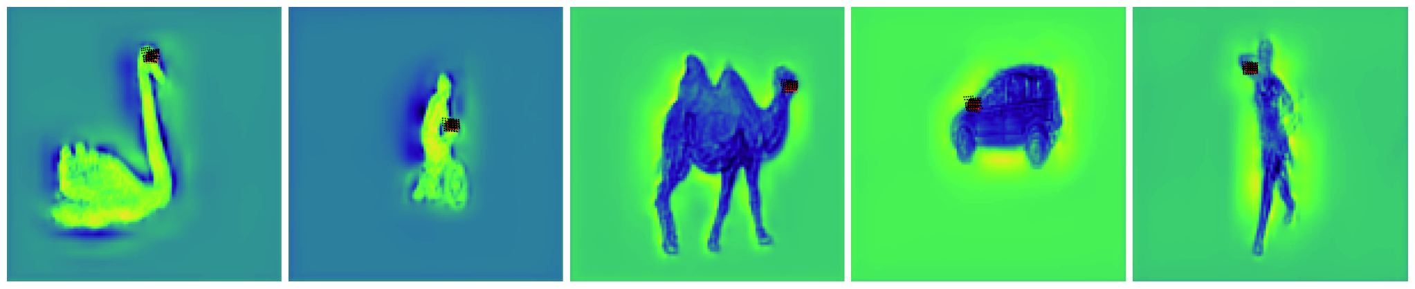
We study the effectiveness of the cascading alignment operation in Eq. 10 by comparing our whole model to one variant in which the deformable convolutional layer is replaced by a regular convolutional kernel. We can draw the following conclusion from results in the sub-table named Cascading Alignment in Table I. The cascading alignment process can achieve an absolute gain of and in mean and mean , respectively. Fig. 9 shows the visualization of sampling positions on immediate features in cascading alignment. We use red points ( points in each feature map) to represent the sampling positions of the regular convolution network, and black points represent the sampling locations of deformable convolution in the cascading alignment. We observe that the sampling positions in the regular convolution are fixed all over the feature map, while they in APM tend to adaptively adjust according to objects’ shape and scale. The quantitative evidence of such adaptive deformation is provided in Table I.
Moreover, we also evaluate the performance of the IMCNet with a different number of cascading layers of alignment. We can see from the results in Cascading Alignment of Table I that the performance gradually improves as the number of cascading layer increases, reaching the best at . Therefore, the default value of is set as 4 for the cascading alignment process.
III-C4 Effectiveness of TSC
To verify the effect of the TSC, we only add a bridge stage, which is implemented by a convolutional layer, between the cascading alignment and segmentation module. As shown in Table I, in the sub-table TSC, the variant without TSC suffers from a significant performance drop ( in mean and in mean ), which verifies the effectiveness of TSC.
III-C5 Comparison of different training strategies
In order to enhance the local dependence during the convergence of training, we introduce a joint training strategy to capture intra-frame discriminability. The joint training strategy helps guarantee our model focuses on mining both local and global dependence. Our IMCNet is trained with our proposed joint training strategy in Stage 2. To investigate the efficacy of joint training strategy on the UVOS task, we train our model with only Stage 1 and Stage 1&Stage 2 w/o. joint training. Its comparison results in Training Strategy of Table I demonstrate the effectiveness of such a joint training method. In Stage 1, our model is trained with a subset of YouTube-VOS (annotated one objects mask), it is not reliable for characterizing objects surrounded by cluttered background (see breakdance in the second row of Fig. 10), leading to poor generalization. Especially, it easily fails in the presence of fast motion (in breakdance and motocross-jump sequences). However, for intra-frame discriminability, it is better than Stage 1 & Stage 2 without joint training, as shown camel in the second and third rows of Fig. 10. The IMCNet which is trained with Stage 1 & Stage 2 (w/o. joint training) is sensitive to similar surroundings and distracting backgrounds, while joint training strategy effectively improves the intra-frame discriminability (see breakdance and camel in the fourth row of Fig. 10).
III-D Influence of key parameters
In this section, we analyze the influence of key parameters in our IMCNet, including the frame number , and interval step , for input frames on a densely annotated dataset. The networks are evaluated using mean region similarity () and mean boundary accuracy ().
III-D1 Frame number
Our IMCNet simultaneously takes frames as inputs and generates the segmentation mask of the center frame (). It is of interest to assess the influence of the number of input frames () on the final performance. Table II shows the results for this. From the results, we can see that the performance can deteriorate as increases. When is larger, it means that the information of frames which are far from the center frame is also considered, which may lead to noisy information. Based on this analysis, the IMCNet achieves the best performance of in mean and in mean when on the dataset.
| Network Variant | val | |||
|---|---|---|---|---|
| Mean | Mean | |||
| Frame Number () | ||||
| 80.2 | -2.5 | 78.5 | -2.6 | |
| 79.7 | -3.0 | 78.0 | -3.1 | |
| Step () | ||||
| 82.6 | -0.1 | 80.8 | -0.3 | |
| 82.0 | -0.7 | 80.2 | -0.9 | |
| 82.7 | - | 81.1 | - | |
| 81.9 | -0.8 | 80.5 | -0.6 | |
| Category | Mean | ||||
|---|---|---|---|---|---|
| Step | |||||
| 1 | 2 | 4 | 6 | ||
| AC | 84.0 | 82.2 | 83.9 | 83.0 | 1.8 |
| BC | 81.6 | 81.8 | 81.9 | 81.5 | 0.4 |
| CS | 84.3 | 84.4 | 84.5 | 84.0 | 0.5 |
| DB | 69.7 | 63.7 | 68.5 | 66.3 | 6.0 |
| DEF | 80.6 | 79.8 | 81.0 | 80.5 | 1.2 |
| EA | 78.5 | 78.8 | 78.6 | 77.4 | 1.4 |
| FM | 78.6 | 76.7 | 78.6 | 77.4 | 1.9 |
| HO | 78.1 | 77.3 | 78.3 | 77.4 | 1.0 |
| IO | 78.3 | 78.7 | 78.7 | 78.3 | 0.4 |
| LR | 80.1 | 80.1 | 80.0 | 78.8 | 1.3 |
| MB | 77.8 | 76.6 | 78.3 | 77.6 | 1.7 |
| OCC | 76.7 | 76.9 | 77.2 | 76.7 | 0.5 |
| OV | 81.2 | 78.0 | 81.3 | 80.7 | 3.3 |
| SC | 71.9 | 72.5 | 72.6 | 72.1 | 0.7 |
| SV | 78.1 | 78.6 | 78.4 | 77.3 | 1.3 |
III-D2 Step
Another key parameter is the step of frames , which decides sequential frames as input in an ordered manner is selected at a fixed-length frame interval . represents selecting three consecutive adjacent video frames in input frames. Step in Table II reports the mean and mean as a function of the frame interval . We can see that when increase, the mean and mean first increase and then decrease.
Moreover, Table III illustrates the performance comparison of different under various video attributes of , including low resolution (LR), scale variation (SV), shape complexity (SC), fast motion (FM), camera-shake (CS), interacting objects (IO), dynamic background (DB), motion blur (MB), deformation (DEF), occlusion (OCC), heterogeneous object (HO), edge ambiguity (EA), out-of-view (OV), appearance change (AC), and background cluttering (BC). IMCNet with has the best performance under most attributes. As a result, in the presence of appearance change (AC), dynamic background (DB), and low resolution (LR), the model with is the most robust due to the primary object(s) undergoing huge appearance change, scale variation, and it is difficult to capture the similarity between multi-frames when is larger. We can reach the same conclusion from in Table III that dynamic background (DB) and out-of-view (OV) have the greatest influence on interval step .
III-E Comparison with state-of-the-arts
We compare our proposed IMCNet with the state-of-the-art methods in two densely annotated video segmentation datasets, i.e., [50] and YouTube-Objects [51]. We apply the training strategy mentioned in §III-B. Input frame numbers and step are set as 3 and 4.
| Method | OF | RGB | MF | |||||||
| Mean | Mean | Recall | Decay | Mean | Recall | Decay | ||||
| SFL [26] | ✓ | ✓ | 67.1 | 67.4 | 81.4 | 6.2 | 66.7 | 77.1 | 5.1 | |
| LMP [35] | ✓ | 68.0 | 70.0 | 85.0 | 1.3 | 65.9 | 79.2 | 2.5 | ||
| FSEG [24] | ✓ | ✓ | 68.0 | 70.7 | 83.0 | 1.5 | 65.3 | 73.8 | 1.8 | |
| LVO [25] | ✓ | ✓ | 74.0 | 75.9 | 89.1 | 0.0 | 72.1 | 83.4 | 1.3 | |
| PDB [36] | ✓ | 75.9 | 77.2 | 90.1 | 0.9 | 74.5 | 84.4 | -0.2 | ||
| MOT [30] | ✓ | ✓ | 77.3 | 77.2 | 87.8 | 5.0 | 77.4 | 84.4 | 3.3 | |
| EPO [32] | ✓ | ✓ | ✓ | 78.1 | 80.6 | 95.2 | 2.2 | 75.5 | 87.9 | 2.4 |
| FEM [33] | ✓ | ✓ | 78.4 | 79.9 | 93.9 | 4.4 | 76.9 | 88.3 | 2.4 | |
| AGS [41] | ✓ | 78.6 | 79.7 | 91.1 | 1.9 | 77.4 | 85.8 | 1.6 | ||
| AGNN [40] | ✓ | ✓ | 79.9 | 80.7 | 94.0 | 0.0 | 79.1 | 90.5 | 0.0 | |
| COS [37] | ✓ | ✓ | 80.0 | 80.5 | 93.1 | 4.4 | 79.4 | 90.4 | 5.0 | |
| COS† [38] | ✓ | ✓ | 80.4 | 81.1 | 93.8 | 5.3 | 79.7 | 91.1 | 5.6 | |
| AnDiff∗ [39] | ✓ | ✓ | 81.1 | 81.7 | 90.9 | 2.2 | 80.5 | 85.1 | 0.6 | |
| DyStaB [34] | ✓ | ✓ | 81.4 | 82.8 | - | - | 80.0 | - | - | |
| WCS [42] | ✓ | ✓ | 81.5 | 82.2 | - | - | 80.7 | - | - | |
| MAT [31] | ✓ | ✓ | 81.6 | 82.4 | 94.5 | 5.5 | 80.7 | 90.2 | 4.5 | |
| DFNet∗[43] | ✓ | ✓ | 82.6 | 83.4 | - | - | 81.8 | - | - | |
| TransportNet [48] | ✓ | ✓ | 84.8 | 84.5 | - | - | 85.0 | - | - | |
| RTNet [49] | ✓ | ✓ | ✓ | 84.2 | 84.8 | 95.8 | - | 83.5 | 93.1 | - |
| Ours | ✓ | ✓ | 81.9 | 82.7 | 94.8 | 3.6 | 81.1 | 88.6 | 3.6 | |
| Ours∗ | ✓ | ✓ | 82.6 | 83.5 | 95.9 | 4.6 | 81.7 | 89.4 | 4.4 | |
- *
Uses multi-scale inference and instance pruning, and our method only uses the former.
-
COS is improved by group attention mechanisms.
III-E1 Evaluation on
Quantitative result.
Table IV shows the detailed results, with several top-performing UVOS methods, including single-modality input methods [26, 35, 36, 37, 38, 39, 40, 41, 42, 43] and multi-modality input models [25, 29, 24, 30, 31, 32, 33, 34, 48, 49] taken from the benchmark. We can observe that our IMCNet achieves competitive performance compared to other methods. As shown in Table IV, our model achieves the third-best results in terms of mean and we can find that IMCNet has achieved the best results in terms of recall value of . Specifically, our IMCNet outperforms all single-modality-based methods and achieves the results on the with over mean , and is equal to the DFNet [43]. In addition, we do not apply CRF post-processing. The results indicate that our model can capture motion information and implicitly compensate motion by the MCM better than the single-modality input method. Multi-modality methods [48, 49] use the optical flow as a cue to segment objects and can better capture the motion information. Therefore, these two multi-modality methods, i.e., TransportNet[48] and RTNet [49], achieved the best results in the UVOS task. Although the multi-modality input methods TransportNet[48] and RTNet [49] have achieved the best result, due to introducing an additional pre-processing stage to predict the optical flow, the number of model parameters is more than our model, and inference time is slower (See §III-E3).

Qualitative results. Fig. 11 depicts the qualitative results on which contains some challenges like cluttered background, deformation, and motion blur, e.g., breakdance, dance-twirl, and horsejump-high. As seen, our IMCNet is robust to these challenges and precisely extracts primary objects(s) with accurate boundaries. The breakdance and dance-twirl sequences from the contain similar surroundings and large deformation. We can find that our method can effectively discriminate the target from those background distractors, thanks to the ACM and APM. Besides, through implicit learned and compensating motion by the MCM, our IMCNet can accurately segment some sequences (e.g., horsejump-high), where there is fast motion and suffer from motion blur.
III-E2 Evaluation on YouTube-Objects
Quantitative result.
Table V reports the results of several compared methods [25, 26, 24, 36, 41, 37, 38, 40, 31, 42] for different categories on the YouTube-Objects dataset. Our method achieves promising performance in most categories and the second-best overall results on mean . It is slightly worse than COS† () in terms of mean and achieves the second-best results. However, we emphasize that the COS† is more computationally expensive. Compared with COS, our IMCNet is superior to the COS without group attention mechanisms. It is indicated that COS obtains a precise segmentation mask by capturing richer structure information of videos, but our IMCNet can achieve sufficient segmentation accuracy through three frames without damaging inference speed.
| Category | LVO [25] | SFL [26] | FSEG [24] | PDB [36] | AGS [41] | COS [37] | COS† [38] | AGNN [40] | MAT [31] | WCS [42] | Ours | Ours∗ |
|---|---|---|---|---|---|---|---|---|---|---|---|---|
| Airplane (6) | 86.2 | 65.6 | 81.7 | 78.0 | 87.7 | 81.1 | 83.4 | 81.1 | 72.9 | 81.8 | 81.2 | 81.1 |
| Bird (6) | 81.0 | 65.4 | 63.8 | 80.0 | 76.7 | 75.7 | 78.1 | 75.9 | 77.5 | 81.2 | 78.3 | 81.1 |
| Boat (15) | 68.5 | 59.9 | 72.3 | 58.9 | 72.2 | 71.3 | 71.0 | 70.7 | 66.9 | 67.6 | 67.9 | 70.3 |
| Car (7) | 69.3 | 64.0 | 74.9 | 76.5 | 78.6 | 77.6 | 79.1 | 78.1 | 79.0 | 79.5 | 78.5 | 77.1 |
| Cat (16) | 58.8 | 58.9 | 68.4 | 63.0 | 69.2 | 66.5 | 66.1 | 67.9 | 73.7 | 65.8 | 70.4 | 73.3 |
| Cow (20) | 68.5 | 51.2 | 68.0 | 64.1 | 64.6 | 69.8 | 69.5 | 69.7 | 67.4 | 66.2 | 67.1 | 66.8 |
| Dog (27) | 61.7 | 54.1 | 69.4 | 70.1 | 73.3 | 76.8 | 76.2 | 77.4 | 75.9 | 73.4 | 73.1 | 74.8 |
| Horse (14) | 53.9 | 64.8 | 60.4 | 67.6 | 64.4 | 67.4 | 71.9 | 67.3 | 63.2 | 69.5 | 63.0 | 64.8 |
| Motorbile (10) | 60.8 | 52.6 | 62.7 | 58.3 | 62.1 | 67.7 | 67.9 | 68.3 | 62.6 | 69.3 | 63.3 | 58.7 |
| Train (5) | 66.3 | 34.0 | 62.2 | 35.2 | 48.2 | 46.8 | 46.5 | 47.8 | 51.0 | 49.7 | 56.8 | 56.8 |
| Mean | 67.5 | 57.1 | 68.4 | 65.2 | 69.7 | 70.1 | 71.0 | 70.4 | 69.0 | 70.4 | 70.0 | 70.5 |
- *
Uses multi-scale inference.
-
COS is improved by group attention mechanisms.
Qualitative results. Fig. 12 shows the qualitative results on YouTube-Objects. We can observe that the target object suffering some challenging scenarios like fast motion (e.g., car-0009 and horse-0011) and large deformation (e.g., dog-0022 and horse-0011). Our model can deal with such challenges well, it verifies the effectiveness of the MCM.

III-E3 Runtime comparison
To further investigate the computation efficiency of our IMCNet, we report the number of network parameters and inference time comparisons on the datasets with a 480p resolution. We do not count data loading and only focus on the segmentation time of the models. We compare the IMCNet with state-of-the-art methods which share their codes or include the corresponding experimental results, including AGNN [40], AnDiff [39], COS [37], MAT [31] DFNet [43], TransportNet [48], and RTNet [49]. For the inference time comparison, we run the public code of other methods and our code on the same conditions with NVIDIA TITAN RTX GPU. The analysis results are summarized in Table VI.
Table VI shows that our IMCNet reduces the model complexity with fewer parameters than the other methods. For the inference comparison, we can observe that our method shows a faster speed than other competitors. Fig. 13 depicts a visualization of the trade-off between accuracy and efficiency of representative methods on the validation set of . As can be seen, our IMCNet achieves the best trade-off.
| Method | AGNN [40] | AnDiff [39] | COS [37] | MAT [31] | DFNet [43] | TransportNet [48] | RTNet1 [49] | Ours |
|---|---|---|---|---|---|---|---|---|
| #Param. (M) | 82.3 | 79.3 | 81.2 | 142.7 | 64.7 | - | 277.2 | 47.9 |
| Inf. Time (s/frame) | 0.53 | 0.35 | 0.45 | 0.05 | 0.28 | 0.28 | 0.25 | 0.05 |
| Mean | 79.9 | 81.1 | 80.0 | 81.6 | 82.6 | 84.8 | 84.2 | 82.6 |
- 1
The RTNet source code only provides a pre-trained model based on ResNet-34, we use the model based on ResNet-34 here.
IV Conclusion
In this paper, we proposed a novel framework, IMCNet, for the UVOS. The proposed IMCNet mines the long-term correlations from several input frames by a light-weight affinity computing module. In addition, an attention propagation module is proposed to transmit global correlation in a top-down manner. Finally, a novel motion compensation module aligns motion information from temporally adjacent frames to the current frame which achieves implicit motion compensation at the feature level. Experimental results demonstrated that the proposed IMCNet achieves favorable performance against other methods while running at a faster speed and using much fewer parameters.
Acknowledgments
This work was supported by the National Nature Science Foundation of China under grant 61620106012 and Beijing Natural Science Foundation under grant 4202042.
References
- [1] V. Mezaris and M. G. Strintzis, “Object segmentation and ontologies for MPEG-2 video indexing and retrieval,” in Image and Video Retrieval, vol. 3115, 2004, pp. 573–581.
- [2] X. Bai and G. Sapiro, “A geodesic framework for fast interactive image and video segmentation and matting,” in Proceedings of the IEEE/CVF International Conference on Computer Vision (ICCV), 2007, pp. 1–8.
- [3] A. Criminisi, T. Sharp, C. Rother, and P. P’erez, “Geodesic image and video editing,” ACM Transactions on Graphics, vol. 29, no. 5, 2010.
- [4] X. Song and G. Fan, “Joint key-frame extraction and object segmentation for content-based video analysis,” IEEE Transactions on Circuits and Systems for Video Technology, vol. 16, no. 7, pp. 904–914, 2006.
- [5] T. Hata, N. Kuwahara, T. Nozawa, D. L. Schwenke, and A. Vetro, “Surveillance system with object-aware video transcoder,” in 2005 IEEE 7th Workshop on Multimedia Signal Processing, 2005, pp. 1–4.
- [6] H. Hadizadeh and I. V. Bajić, “Saliency-aware video compression,” IEEE Transactions on Image Processing, vol. 23, no. 1, pp. 19–33, 2014.
- [7] Y. Liu, Z. Li, and Y. Soh, “Region-of-interest based resource allocation for conversational video communication of h.264/avc,” IEEE Transactions on Circuits and Systems for Video Technology, vol. 18, no. 1, pp. 134–139, 2008.
- [8] Y. Liu, Z. G. Li, and Y. C. Soh, “A novel rate control scheme for low delay video communication of h.264/avc standard,” IEEE Transactions on Circuits and Systems for Video Technology, vol. 17, no. 1, pp. 68–78, 2007.
- [9] Z. Li, C. Zhu, N. Ling, X. Yang, G. Feng, S. Wu, and F. Pan, “A unified architecture for real-time video-coding systems,” IEEE Transactions on Circuits and Systems for Video Technology, vol. 13, no. 6, pp. 472–487, 2003.
- [10] Z. Li, F. Pan, G. Feng, K. P. Lim, X. Lin, and S. Rahardja, “Adaptive basic unit layer rate control for jvt,” in JVT 7th Meeting, Pattaya, Mar2003, 2003, JVT-G012.
- [11] S. Caelles, K.-K. Maninis, J. Pont-Tuset, L. Leal-Taixé, D. Cremers, and L. Van Gool, “One-shot video object segmentation,” in Proceedings of the IEEE/CVF Conference on Computer Vision and Pattern Recognition (CVPR), 2017, pp. 5320–5329.
- [12] F. Perazzi, A. Khoreva, R. Benenson, B. Schiele, and A. Sorkine-Hornung, “Learning video object segmentation from static images,” in Proceedings of the IEEE/CVF Conference on Computer Vision and Pattern Recognition (CVPR), 2017, pp. 3491–3500.
- [13] C. Ventura, M. Bellver, A. Girbau, A. Salvador, F. Marques, and X. Giro-i Nieto, “RVOS: End-to-end recurrent network for video object segmentation,” in Proceedings of the IEEE/CVF Conference on Computer Vision and Pattern Recognition (CVPR), 2019, pp. 5272–5281.
- [14] Z. Liu, J. Liu, W. Chen, X. Wu, and Z. Li, “FAMINet: Learning real-time semisupervised video object segmentation with steepest optimized optical flow,” IEEE Transactions on Instrumentation and Measurement, vol. 71, pp. 1–16, 2022.
- [15] P. Huang, J. Han, N. Liu, J. Ren, and D. Zhang, “Scribble-supervised video object segmentation,” IEEE/CAA Journal of Automatica Sinica, vol. 9, no. 2, pp. 339–353, 2022.
- [16] D. Zhang, J. Han, L. Yang, and D. Xu, “SPFTN: A joint learning framework for localizing and segmenting objects in weakly labeled videos,” IEEE Transactions on Pattern Analysis and Machine Intelligence, vol. 42, no. 2, pp. 475–489, 2020.
- [17] Q. Lai, S. Khan, Y. Nie, H. Sun, J. Shen, and L. Shao, “Understanding more about human and machine attention in deep neural networks,” IEEE Transactions on Multimedia, vol. 23, pp. 2086–2099, 2021.
- [18] Q. Hou, M.-M. Cheng, X. Hu, A. Borji, Z. Tu, and P. H. S. Torr, “Deeply supervised salient object detection with short connections,” IEEE Transactions on Pattern Analysis and Machine Intelligence, vol. 41, no. 4, pp. 815–828, 2019.
- [19] N. Liu, J. Han, and M.-H. Yang, “PiCANet: Pixel-wise contextual attention learning for accurate saliency detection,” IEEE Transactions on Image Processing, vol. 29, pp. 6438–6451, 2020.
- [20] T. Wang, L. Zhang, S. Wang, H. Lu, G. Yang, X. Ruan, and A. Borji, “Detect globally, refine locally: A novel approach to saliency detection,” in Proceedings of the IEEE/CVF Conference on Computer Vision and Pattern Recognition (CVPR), 2018, pp. 3127–3135.
- [21] A. Faktor and M. Irani, “Video segmentation by non-local consensus voting,” in Proceedings of the British Machine Vision Conference, 2014, pp. 21.1–21.12.
- [22] Q. Fan, F. Zhong, D. Lischinski, D. Cohen-Or, and B. Chen, “JumpCut: Non-successive mask transfer and interpolation for video cutout,” ACM Trans. Graph., vol. 34, no. 6, pp. 1–10, 2015.
- [23] B. Luo, H. Li, F. Meng, Q. Wu, and K. N. Ngan, “An unsupervised method to extract video object via complexity awareness and object local parts,” IEEE Transactions on Circuits and Systems for Video Technology, vol. 28, no. 7, pp. 1580–1594, 2018.
- [24] S. D. Jain, B. Xiong, and K. Grauman, “FusionSeg: Learning to combine motion and appearance for fully automatic segmentation of generic objects in videos,” in Proceedings of the IEEE/CVF Conference on Computer Vision and Pattern Recognition (CVPR), 2017, pp. 2117–2126.
- [25] P. Tokmakov, K. Alahari, and C. Schmid, “Learning video object segmentation with visual memory,” in Proceedings of the IEEE International Conference on Computer Vision (ICCV), Oct 2017, pp. 4491–4500.
- [26] J. Cheng, Y.-H. Tsai, S. Wang, and M.-H. Yang, “SegFlow: Joint learning for video object segmentation and optical flow,” in Proceedings of the IEEE/CVF International Conference on Computer Vision (ICCV), 2017, pp. 686–695.
- [27] J. Han, L. Yang, D. Zhang, X. Chang, and X. Liang, “Reinforcement cutting-agent learning for video object segmentation,” in Proceedings of the IEEE Conference on Computer Vision and Pattern Recognition (CVPR), 2018, pp. 9080–9089.
- [28] S. N. Gowda, P. Eustratiadis, T. M. Hospedales, and L. Sevilla-Lara, “ALBA : Reinforcement learning for video object segmentation,” CoRR, vol. abs/2005.13039, 2020.
- [29] P. Tokmakov, C. Schmid, and K. Alahari, “Learning to segment moving objects,” International Journal of Computer Vision, vol. 127, no. 3, pp. 282–301, 2019.
- [30] M. Siam, C. Jiang, S. Lu, L. Petrich, M. Gamal, M. Elhoseiny, and M. Jagersand, “Video object segmentation using teacher-student adaptation in a human robot interaction (HRI) setting,” in 2019 International Conference on Robotics and Automation (ICRA), 2019, pp. 50–56.
- [31] T. Zhou, J. Li, S. Wang, R. Tao, and J. Shen, “MATNet: Motion-attentive transition network for zero-shot video object segmentation,” IEEE Transactions on Image Processing, vol. 29, pp. 8326–8338, 2020.
- [32] M. Faisal, I. Akhter, M. Ali, and R. Hartley, “EpO-Net: Exploiting geometric constraints on dense trajectories for motion saliency,” in Proceedings of the IEEE/CVF Winter Conference on Applications of Computer Vision (WACV), 2020, pp. 1873–1882.
- [33] Y. Zhou, X. Xu, F. Shen, X. Zhu, and H. T. Shen, “Flow-edge guided unsupervised video object segmentation,” IEEE Transactions on Circuits and Systems for Video Technology, pp. 1–1, 2021.
- [34] Y. Yang, B. Lai, and S. Soatto, “DyStaB: Unsupervised object segmentation via dynamic-static bootstrapping,” in Proceedings of the IEEE/CVF Conference on Computer Vision and Pattern Recognition (CVPR), June 2021, pp. 2826–2836.
- [35] P. Tokmakov, K. Alahari, and C. Schmid, “Learning motion patterns in videos,” in Proceedings of the IEEE Conference on Computer Vision and Pattern Recognition (CVPR), July 2017, pp. 531–539.
- [36] H. Song, W. Wang, S. Zhao, J. Shen, and K.-M. Lam, “Pyramid dilated deeper convlstm for video salient object detection,” in Proceedings of the European Conference on Computer Vision (ECCV), September 2018, pp. 744–760.
- [37] X. Lu, W. Wang, C. Ma, J. Shen, L. Shao, and F. Porikli, “See more, know more: Unsupervised video object segmentation with co-attention siamese networks,” in Proceedings of the IEEE/CVF Conference on Computer Vision and Pattern Recognition (CVPR), 2019, pp. 3618–3627.
- [38] X. Lu, W. Wang, J. Shen, D. Crandall, and J. Luo, “Zero-shot video object segmentation with co-attention siamese networks,” IEEE Transactions on Pattern Analysis and Machine Intelligence, vol. 44, no. 4, pp. 2228–2242, 2022.
- [39] Z. Yang, Q. Wang, L. Bertinetto, S. Bai, W. Hu, and P. Torr, “Anchor diffusion for unsupervised video object segmentation,” in Proceedings of the IEEE/CVF International Conference on Computer Vision (ICCV), 2019, pp. 931–940.
- [40] W. Wang, X. Lu, J. Shen, D. Crandall, and L. Shao, “Zero-shot video object segmentation via attentive graph neural networks,” in Proceedings of the IEEE/CVF International Conference on Computer Vision (ICCV), 2019, pp. 9235–9244.
- [41] W. Wang, H. Song, S. Zhao, J. Shen, S. Zhao, S. C. H. Hoi, and H. Ling, “Learning unsupervised video object segmentation through visual attention,” in Proceedings of the IEEE/CVF Conference on Computer Vision and Pattern Recognition (CVPR), 2019, pp. 3059–3069.
- [42] L. Zhang, J. Zhang, Z. Lin, R. Měch, H. Lu, and Y. He, “Unsupervised video object segmentation with joint hotspot tracking,” in Proceedings of the European Conference on Computer Vision (ECCV), 2020, pp. 490–506.
- [43] M. Zhen, S. Li, L. Zhou, J. Shang, H. Feng, T. Fang, and L. Quan, “Learning discriminative feature with CRF for unsupervised video object segmentation,” in Proceedings of the European Conference on Computer Vision (ECCV), 2020, pp. 445–462.
- [44] C. Xiong, V. Zhong, and R. Socher, “Dynamic coattention networks for question answering,” CoRR, vol. abs/1611.01604, 2016.
- [45] J. Lu, J. Yang, D. Batra, and D. Parikh, “Hierarchical question-image co-attention for visual question answering,” in Proceedings of the 30th International Conference on Neural Information Processing Systems, vol. 29, 2016, p. 289–297.
- [46] J. Dai, H. Qi, Y. Xiong, Y. Li, G. Zhang, H. Hu, and Y. Wei, “Deformable convolutional networks,” in Proceedings of the IEEE/CVF International Conference on Computer Vision (ICCV), 2017, pp. 764–773.
- [47] X. Zhu, H. Hu, S. Lin, and J. Dai, “Deformable convnets V2: More deformable, better results,” in Proceedings of the IEEE/CVF Conference on Computer Vision and Pattern Recognition (CVPR), 2019, pp. 9300–9308.
- [48] K. Zhang, Z. Zhao, D. Liu, Q. Liu, and B. Liu, “Deep transport network for unsupervised video object segmentation,” in Proceedings of the IEEE/CVF International Conference on Computer Vision (ICCV), October 2021, pp. 8781–8790.
- [49] S. Ren, W. Liu, Y. Liu, H. Chen, G. Han, and S. He, “Reciprocal transformations for unsupervised video object segmentation,” in Proceedings of the IEEE/CVF Conference on Computer Vision and Pattern Recognition (CVPR), June 2021, pp. 15 455–15 464.
- [50] F. Perazzi, J. Pont-Tuset, B. McWilliams, L. Van Gool, M. Gross, and A. Sorkine-Hornung, “A benchmark dataset and evaluation methodology for video object segmentation,” in Proceedings of the IEEE Conference on Computer Vision and Pattern Recognition (CVPR), June 2016, pp. 724–732.
- [51] A. Prest, C. Leistner, J. Civera, C. Schmid, and V. Ferrari, “Learning object class detectors from weakly annotated video,” in Proceedings of the IEEE Conference on Computer Vision and Pattern Recognition (CVPR), 2012, pp. 3282–3289.
- [52] O. Russakovsky, J. Deng, H. Su, J. Krause, S. Satheesh, S. Ma, Z. Huang, A. Karpathy, A. Khosla, M. Bernstein, A. C. Berg, and L. Fei-Fei, “ImageNet large scale visual recognition challenge,” International Journal of Computer Vision, vol. 115, no. 3, p. 211–252, Dec. 2015.
- [53] L. Wang, H. Lu, Y. Wang, M. Feng, D. Wang, B. Yin, and X. Ruan, “Learning to detect salient objects with image-level supervision,” in Proceedings of the IEEE Conference on Computer Vision and Pattern Recognition (CVPR), July 2017, pp. 3796–3805.
- [54] K. He, X. Zhang, S. Ren, and J. Sun, “Deep residual learning for image recognition,” in Proceedings of the IEEE Conference on Computer Vision and Pattern Recognition (CVPR), June 2016, pp. 770–778.
- [55] T.-Y. Lin, P. Dollar, R. Girshick, K. He, B. Hariharan, and S. Belongie, “Feature pyramid networks for object detection,” in Proceedings of the IEEE Conference on Computer Vision and Pattern Recognition (CVPR), July 2017, pp. 936–944.
- [56] S. Woo, J. Park, J.-Y. Lee, and I. S. Kweon, “CBAM: Convolutional block attention module,” in Proceedings of the European Conference on Computer Vision (ECCV), September 2018, pp. 3–19.
- [57] X. Qin, Z. Zhang, C. Huang, C. Gao, M. Dehghan, and M. Jagersand, “BASNet: Boundary-aware salient object detection,” in Proceedings of the IEEE/CVF Conference on Computer Vision and Pattern Recognition (CVPR), June 2019, pp. 7471–7481.
- [58] P.-T. de Boer, K. D. P., S. Mannor, and R. Y. Rubinstein, “A tutorial on the cross-entropy method,” Annals of Operations Research, vol. 134, pp. 19–67, 2005.
- [59] Z. Wang, A. Bovik, H. Sheikh, and E. Simoncelli, “Image quality assessment: from error visibility to structural similarity,” IEEE Transactions on Image Processing, vol. 13, no. 4, pp. 600–612, 2004.
- [60] J. Yu, Y. Jiang, Z. Wang, Z. Cao, and T. Huang, “Unitbox: An advanced object detection network,” in Proceedings of the 24th ACM International Conference on Multimedia, 2016, p. 516–520.
- [61] N. Xu, L. Yang, Y. Fan, J. Yang, D. Yue, Y. Liang, B. Price, S. Cohen, and T. Huang, “YouTube-VOS: Sequence-to-sequence video object segmentation,” in Proceedings of the European Conference on Computer Vision (ECCV), September 2018, pp. 603–619.
- [62] D. P. Kingma and J. Ba, “Adam: A method for stochastic optimization,” arXiv preprint arXiv:1412.6980, 2014.
- [63] A. Paszke, S. Gross, F. Massa, A. Lerer, J. Bradbury, G. Chanan, T. Killeen, Z. Lin, N. Gimelshein, L. Antiga, A. Desmaison, A. Kopf, E. Yang, Z. DeVito, M. Raison, A. Tejani, S. Chilamkurthy, B. Steiner, L. Fang, J. Bai, and S. Chintala, “PyTorch: An imperative style, high-performance deep learning library,” in Advances in Neural Information Processing Systems, vol. 32, 2019, p. 8024–8035.