跳到论文正文
W Papers独立论文阅读器 arXiv:2204.02409 论文正文 计算阅读时间 · 0%
引用这篇论文根据当前论文元数据生成,正式投稿前建议核对。


License: arXiv.org perpetual non-exclusive license
arXiv:2204.02409v2 [cond-mat.mes-hall] 04 May 2022

Valley hydrodynamics in gapped graphene

Ryotaro Sano Email: sano.ryotaro.52v@st.kyoto-u.ac.jp Affiliation: Department of Physics, Kyoto University, Kyoto 606-8502, Japan    Daigo Oue Affiliation: Department of Physics, Kyoto University, Kyoto 606-8502, Japan Affiliation: The Blackett Laboratory, Department of Physics, Imperial College London, Prince Consort Road, Kensington, London SW7 2AZ, United Kingdom Affiliation: Kavli Institute for Theoretical Sciences, University of Chinese Academy of Sciences, Beijing, 100190, China.    Mamoru Matsuo Affiliation: Kavli Institute for Theoretical Sciences, University of Chinese Academy of Sciences, Beijing, 100190, China. Affiliation: CAS Center for Excellence in Topological Quantum Computation, University of Chinese Academy of Sciences, Beijing 100190, China Affiliation: RIKEN Center for Emergent Matter Science (CEMS), Wako, Saitama 351-0198, Japan Affiliation: Advanced Science Research Center, Japan Atomic Energy Agency, Tokai, 319-1195, Japan
August 11, 2026
Abstract

Recent experiments have revealed that novel nonequilibrium states consistent with the hydrodynamic description of electrons are realized in ultrapure graphene, which hosts the valley degrees of freedom. Here, we formulate a theory of electron hydrodynamics including dissipation processes of the valley angular momentum by employing the concept of micropolar fluids. As a result, our theory proposes a novel strategy to generate a valley polarization by the microrotation. We uncover that the rotational viscosity induces longitudinal valley currents which are second order in electric fields.

Introduction.— The investigation of internal quantum degrees of freedom (DOF) of electrons in solids lies at the heart of condensed matter physics. The most-studied example is that of the electron spin, which gives rise to the vast field of spintronics with an eye on their potential for future electronics Wolf et al. 2001; Maekawa et al. 2017. The advent of novel 2D materials which support massive Dirac fermions, exemplified by gapped graphene and transition metal dichalcogenides, has triggered research on alternative future electronics Xiao et al. 2007; Yao et al. 2008; Xiao et al. 2012; Butler et al. 2013; Nguyen and Nguyen 2016; Liu et al. 2017; Choi et al. 2017. In these systems, two inequivalent valleys KK and −K-K reside at the corners of the hexagonal Brillouin zone. Similar to the spin, the valley labeling constitutes a discrete angular momentum for low energy carriers. From this point of view, the valley DOF has a potential use for information carriers, giving rise to an active research field called valleytronics as a promising concept for the next-generation electronics Rycerz et al. 2007; Radisavljevic et al. 2011; Wang et al. 2012; Xu et al. 2014; Zhang et al. 2014; Schaibley et al. 2016; Vitale et al. 2018; Liu et al. 2019. Especially, the valley polarization, a nonequilibrium charge carrier imbalance between valleys, is the key to create valleytronic devices Cao et al. 2012; Zeng et al. 2012; Mak et al. 2012; Mak and Shan 2016; Ye et al. 2017; Mak et al. 2018; Li et al. 2014; MacNeill et al. 2015; Srivastava et al. 2015; Aivazian et al. 2015; Back et al. 2017; Mak et al. 2014; Gorbachev et al. 2014; Ye et al. 2016. Therefore, a necessary requirement for valleytronic applications is the ability to generate and control the valley polarization.

Ultraclean 2D materials have also boosted the study of electron hydrodynamics, where electron-electron collisions are the dominant scattering processes. In fact, many pieces of clear evidence for hydrodynamic behaviors of charge carriers have been provided on graphene Crossno et al. 2016; Bandurin et al. 2016; Bandurin et al. 2018; Krishna Kumar et al. 2017; Pellegrino et al. 2017; Berdyugin et al. 2019; Sulpizio et al. 2019; Gallagher et al. 2019; Polini and Geim 2020; Ku et al. 2020; Jenkins et al. 2020; Geurs et al. 2020; Samaddar et al. 2021; Kumar et al. 2021. These nonequilibrium behaviors of interacting systems close to equilibrium are well described by tracking the evolution of conserved quantities including internal microscopic DOF. However, the construction of hydrodynamics which deals with quantum DOF of electrons such as spin and valley is a nontrivial task. This is because dissipation processes of such an angular momentum cannot be captured by those of the vorticity, which follow directly from the momentum conservation law 11 1 More detailed discussion is given in the supplemental materials. Thus, electron hydrodynamics reaches the stage of going beyond the conventional Navier-Stokes equation.

Refer to caption
Figure 1: Schematics of the microrotation in valley hydrodynamics. The non-uniform velocity 𝒖​(𝒓){\bf\it u}({\bf\it r}) gives rise to the vorticity ∇×𝒖\nabla\times{\bf\it u}. On the other hand, the microrotation 𝝎{\bf\it\omega} is the internal angular momentum stems from the valley polarization PvP_{\mathrm{v}} of fluid elements. The microrotation relaxes towards the vorticity due to the rotational viscosity.

The concept of micropolar fluids gives a new twist to the previous studies of electron hydrodynamics. Micropolar fluid is an extended fluid with an internal rotation of fluid elements so-called the microrotation [see Fig.1]. In micropolar fluids, the antisymmetric components of the stress tensor play a crucial role in dissipation processes of angular momentum, thereby switching on the rotational viscosity between the vorticity and the microrotation ERINGEN 1966; Eringen 1999; Eringen 2001; Łukaszewicz 1999. These features have led to special attention in micropolar fluids due to their many applications in liquid crystals Chandrasekhar et al. 1992; de Gennes and Prost 1993, ferrofluids Odenbach 2002; Shliomis 1972; Rosensweig 2013, spintronics Takahashi et al. 2016, and active matter Marchetti et al. 2013; Markovich et al. 2019; Markovich and Lubensky 2021; Shaik and Elfring 2021. Furthermore, the phenomenon of angular momentum conversion between internal DOF of quantum particles and mechanical rotation have attracted great interest in various fields, ranging from nuclear physics Adamczyk et al. 2017; Florkowski et al. 2018; Hattori et al. 2019 to condensed matter physics Matsuo et al. 2013; Matsuo et al. 2017; Kobayashi et al. 2017; Hughes et al. 2011. This naturally motivates us to study electron hydrodynamics including internal quantum DOF, especially the valley angular momentum, with employing the framework of micropolar fluids. Our study proposes a new strategy for controlling the valley polarization by the microrotation and may open up various avenues for research on valley hydrodynamics.

In this Letter, we derive the hydrodynamic equations with the valley DOF for noncentrosymmetric 2D honeycomb lattice systems, which are correct up to the first order in the drift velocity and the microrotation. We identify the valley DOF as a microrotation and reveal that our theory acquires an emergent conservation law for the microrotation owing to the valley-microrotation coupling. From a symmetry viewpoint, we find that this interaction can appear only in the systems without inversion symmetry. A key ingredient for valleytronics is a controllable way of population imbalance between the two valleys, thereby producing a valley polarization. While previous works showed that a valley polarization can be controlled by optical Cao et al. 2012; Zeng et al. 2012; Mak et al. 2012; Mak and Shan 2016; Ye et al. 2017; Mak et al. 2018, magnetic Li et al. 2014; MacNeill et al. 2015; Srivastava et al. 2015; Aivazian et al. 2015; Back et al. 2017 and electrical Mak et al. 2014; Gorbachev et al. 2014; Ye et al. 2016 means. Our study shows a microfluidic approach to generate such a valley polarization by the microrotation. We also predict nonlinear valley dynamics including longitudinal valley currents [Fig.2] and a circular dichroic valley polarization induced by off-resonant light [Fig.3].

Formulation.— We outline how to derive the hydrodynamic equations for noncentrosymmetric graphene with a staggered sublattice potential. We start from the Boltzmann equation which governs the evolution of the electron distribution function fα​τf_{\alpha\tau} for band α\alpha and valley τ\tau,

∂fα​τ∂t+𝒓˙α​τ⋅∂fα​τ∂𝒓+𝒌˙α​τ⋅∂fα​τ∂𝒌\displaystyle\frac{\partial f_{\alpha\tau}}{\partial t}+\dot{{\bf\it r}}_{\alpha\tau}\cdot\frac{\partial f_{\alpha\tau}}{\partial{\bf\it r}}+\dot{{\bf\it k}}_{\alpha\tau}\cdot\frac{\partial f_{\alpha\tau}}{\partial{\bf\it k}}
=−fα​τ−fα​τNτN−fα​τ−f0τR−fα​τ−fα−ττvf,\displaystyle=-\frac{f_{\alpha\tau}-f_{\alpha\tau}^{\mathrm{N}}}{\tau_{\mathrm{N}}}-\frac{f_{\alpha\tau}-f_{0}}{\tau_{\mathrm{R}}}-\frac{f_{\alpha\tau}-f_{\alpha-\tau}}{\tau_{\mathrm{vf}}}, (1)

where f0f_{0} is the Fermi-Dirac (global equilibrium) distribution function. τN\tau_{\mathrm{N}}, τR\tau_{\mathrm{R}} and τvf\tau_{\mathrm{vf}} are the relaxation times for normal (N), resistive (R) and valley flipping processes. Here, N process conserves the linear momentum, while R process does not. If we construct an electron wave packet near the valley center, the semiclassical equations of motion read Xiao et al. 2010

𝒓˙α​τ=1ℏ​∂ϵα​τ∂𝒌−𝒌˙α​τ×𝜴α​τ,𝒌˙α​τ=−eℏ​𝑬,\displaystyle\dot{{\bf\it r}}_{\alpha\tau}=\frac{1}{\hbar}\frac{\partial\epsilon_{\alpha\tau}}{\partial{\bf\it k}}-\dot{{\bf\it k}}_{\alpha\tau}\times{\bf\it\Omega}_{\alpha\tau},\quad\dot{{\bf\it k}}_{\alpha\tau}=-\frac{e}{\hbar}{\bf\it E}, (2)

where electric fields 𝑬{\bf\it E} can be time-dependent. ϵα​τ​(𝒌)\epsilon_{\alpha\tau}({\bf\it k}) and 𝜴α​τ​(𝒌){\bf\it\Omega}_{\alpha\tau}({\bf\it k}) are the band energy and the Berry curvature of the Bloch electrons respectively. Due to the lack of inversion symmetry, 𝜴α​τ{\bf\it\Omega}_{\alpha\tau} is allowed to have nonzero values for any 𝒌{\bf\it k}.

Following the standard approach Lifshitz and Pitaevskii 1981; Lucas and Fong 2018; Narozhny 2019; Narozhny and Schütt 2019; Narozhny and Gornyi 2021; Kiselev and Schmalian 2020, the continuity equations for the carrier density and the linear momentum are obtained as follows:

∂n∂t+∇⋅𝒋=0,\displaystyle\frac{\partial n}{\partial t}+\nabla\cdot{\bf\it j}=0, (3)
∂Pi∂t+∂Πi​j∂xj=−e​n​Ei−PiτR,\displaystyle\frac{\partial P_{i}}{\partial t}+\frac{\partial\Pi_{ij}}{\partial x_{j}}=-enE_{i}-\frac{P_{i}}{\tau_{\mathrm{R}}}, (4)

where nn and 𝑷{\bf\it P} are the carrier and the linear momentum densities respectively, −e​n​𝑬-en{\bf\it E} is the driving force due to external electric fields. In Eqs.(3) and (4), 𝒋{\bf\it j} and Πi​j\Pi_{ij} are the corresponding fluxes of each density.

A monolayer graphene with a staggered sublattice potential breaking the inversion symmetry is a concrete example for considering valley hydrodynamics. Staggered sublattice potential is generally expected in epitaxial graphene on SiC substrates Berger et al. 2004; Zhou et al. 2007; Tromp and Hannon 2009; Hupalo et al. 2009; Jariwala et al. 2011; Jeon et al. 2013; Nevius et al. 2015. The effective Hamiltonian describing electron states in the vicinity of the KK and −K-K points is given by Xiao et al. 2007

Hτ=a​t​(τ​kx​σx+ky​σy)+Δ2​σz,H_{\tau}=at(\tau k_{x}\sigma_{x}+k_{y}\sigma_{y})+\frac{\Delta}{2}\sigma_{z}, (5)

where aa and tt are the lattice constant and the nearest-neighbor hopping parameter, 𝒌=(kx,ky){\bf\it k}=(k_{x},k_{y}) are the two components of the wave vector measured from the valley center, 𝝈{\bf\it\sigma}’s are the Pauli matrices representing a pseudospin from the sublattice DOF, and τ=±1\tau=\pm 1 is the valley index labeling the two inequivalent valleys. Note that its band structure ϵα​τ​(𝒌)\epsilon_{\alpha\tau}({\bf\it k}) has no dependence on the valley, while the Berry curvature Ωα​τz​(𝒌)\Omega_{\alpha\tau}^{z}({\bf\it k}) has a valley-contrasting property. Because of large separation of two valleys in the momentum space, intervalley scatterings are strongly suppressed Morozov et al. 2006; Morpurgo and Guinea 2006; Gorbachev et al. 2007, implying the potential for regarding the valley polarization as a conserved quantity. Therefore, the effective hydrodynamic theory acquires an emergent continuity equation for the valley polarization:

∂Pv∂t+∇⋅𝒋v=−PvτR−2​Pvτvf,\frac{\partial P_{\mathrm{v}}}{\partial t}+\nabla\cdot{\bf\it j}_{\mathrm{v}}=-\frac{P_{\mathrm{v}}}{\tau_{\mathrm{R}}}-\frac{2P_{\mathrm{v}}}{\tau_{\mathrm{vf}}}, (6)

where PvP_{\mathrm{v}} and 𝒋v{\bf\it j}_{\mathrm{v}} are the valley polarization and the valley current. Here, we have defined the valley polarization Pv≡nK−n−KP_{\mathrm{v}}\equiv n_{K}-n_{-K} as a population imbalance between the two valleys in analogy to the spin polarization. We should note that not only valley flipping processes but also R process contribute to the relaxation of the valley polarization. This indicates that the valley DOF combines a linear momentum and an angular momentum.

In hydrodynamic regime, τN≪τR,τvf\tau_{\mathrm{N}}\ll\tau_{\mathrm{R}},\tau_{\mathrm{vf}}, the system reaches local equilibrium via N electron-electron scatterings, which conserve both the linear momentum and the valley polarization of the electron system. For this reason, we assume that the distribution functions are described as

fα​τN=[exp⁡(ϵα​τ−ℏ​𝒌⋅𝒖−τ​ℏ​ωz−μkB​T)+1]−1,f^{\mathrm{N}}_{\alpha\tau}=\left[\exp\left(\frac{\epsilon_{\alpha\tau}-\hbar{\bf\it k}\cdot{\bf\it u}-\tau\hbar\omega_{z}-\mu}{k_{\mathrm{B}}T}\right)+1\right]^{-1}, (7)

which is referred to as the local equilibrium distribution function. Here, the drift velocity 𝒖{\bf\it u} and the microrotation ωz\omega_{z} are corresponding parameters for conserved quantities 𝑷{\bf\it P} and PvP_{\mathrm{v}}. From a symmetry viewpoint, the absence of inversion symmetry allows for the interplay between the valley DOF and an angular momentum; examples include the spin-valley coupling Xiao et al. 2012; Sanchez et al. 2016 and the valley-vorticity coupling Ominato et al. 2021. Here, the microrotation is the internal angular momentum of the fluid elements and we referred to τ​ωz\tau\omega_{z} as the valley-microrotation coupling.

Since the relevant conduction and valence bands are well described by Eq.(S.61) for low doping level, we use a quadratic dispersion ϵα​τ=α⁡[Δ/2+ℏ2​𝒌2/2​m∗]\epsilon_{\alpha\tau}=\alpha[\Delta/2+\hbar^{2}{\bf\it k}^{2}/2m^{\ast}] with an effective mass m∗≡ℏ2​Δ/2​a2​t2m^{\ast}\equiv\hbar^{2}\Delta/2a^{2}t^{2} in the vicinity of the KK and −K-K points in the following analysis. Under this assumption, we obtain the valley polarization and the valley current in terms of hydrodynamic variables:

Pv\displaystyle P_{\mathrm{v}} =ℏ​ωz​∑α,τ∫[𝑑𝒌]​(−∂f0∂ϵ)≃ℏ​ωz​D​(μ),\displaystyle=\hbar\omega_{z}\sum_{\alpha,\tau}\int[\mathrm{d}{\bf\it k}]\left(-\frac{\partial f_{0}}{\partial\epsilon}\right)\simeq\hbar\omega_{z}D(\mu), (8)
𝒋v\displaystyle{\bf\it j}_{\mathrm{v}} =Pv​𝒖+eℏ​𝑬×∑α,ττ​∫[𝑑𝒌]​𝜴α​τ​f0,\displaystyle=P_{\mathrm{v}}{\bf\it u}+\frac{e}{\hbar}{\bf\it E}\times\sum_{\alpha,\tau}\tau\int[\mathrm{d}{\bf\it k}]{\bf\it\Omega}_{\alpha\tau}f_{0}, (9)

with the density of states D⁡(ϵ)D(\epsilon) and ∫[𝑑𝒌]≡∫𝑑𝒌/(2​π)2\int[\mathrm{d}{\bf\it k}]\equiv\int\mathrm{d}{\bf\it k}/(2\pi)^{2}. These results indicate that the microrotation leads to a valley polarization. The second term in Eq. (9) is the well-known valley Hall effect Xiao et al. 2007, on the other hand, the first term is the longitudinal valley current which is one of our main results.

Combining the valley polarization conservation law Eq. (6) with Eqs. (8) and (9), we end up with the hydrodynamic equations:

∂𝒖∂t+(𝒖⋅∇)𝒖+1ρ∇p=−e​n​𝑬ρ−𝒖τR,\displaystyle\frac{\partial{\bf\it u}}{\partial t}+({\bf\it u}\cdot\nabla){\bf\it u}+\frac{1}{\rho}\nabla p=-\frac{en{\bf\it E}}{\rho}-\frac{{\bf\it u}}{\tau_{\mathrm{R}}}, (10)
∂ωz∂t+(𝒖⋅∇)ωz+ωz(∇⋅𝒖)=−ωzτinter,\displaystyle\frac{\partial\omega_{z}}{\partial t}+({\bf\it u}\cdot\nabla)\omega_{z}+\omega_{z}(\nabla\cdot{\bf\it u})=-\frac{\omega_{z}}{\tau_{\mathrm{inter}}}, (11)

where ρ\rho is the mass density and τinter=(1/τR+2/τvf)−1\tau_{\mathrm{inter}}=(1/\tau_{\mathrm{R}}+2/\tau_{\mathrm{vf}})^{-1} is the relaxation time for intervalley scatterings. Notably, our theory acquires an emergent conservation law for the microrotation and therefore it has a close analogy to micropolar fluids.

In the following analysis, we assume that the fluid is incompressible. We also phenomelogically introduce the rotational viscous torques proportional to the deviation of the microrotation 𝝎{\bf\it\omega} from the vorticity ∇×𝒖/2\nabla\times{\bf\it u}/2. According to Refs. ERINGEN 1966; Eringen 1999; Eringen 2001; Łukaszewicz 1999, the equations governing the flow of incompressible micropolar fluids are given by

D​𝒖D​t=(ν+νr)Δ𝒖+2νr∇×𝝎−e​n​𝑬ρ−𝒖τR,\displaystyle\frac{D{\bf\it u}}{Dt}=(\nu+\nu_{r})\Delta{\bf\it u}+2\nu_{r}\nabla\times{\bf\it\omega}-\frac{en{\bf\it E}}{\rho}-\frac{{\bf\it u}}{\tau_{\mathrm{R}}}, (12)
I​D​ωzD​t=2​νr​[(∇×𝒖)z−2​ωz]−I​ωzτinter,\displaystyle I\frac{D\omega_{z}}{Dt}=2\nu_{r}[(\nabla\times{\bf\it u})_{z}-2\omega_{z}]-I\frac{\omega_{z}}{\tau_{\mathrm{inter}}}, (13)

where D/Dt=∂/∂t+𝒖⋅∇D/Dt=\partial/\partial t+{\bf\it u}\cdot\nabla is the convective derivative. ν\nu and νr\nu_{r} are the kinematic and the rotational viscosities respectively. Here we have introduced the microinertia II, which is moment of inertia per unit fluid mass. In valley hydrodynamics, the motion of electron fluids is described by the drift velocity 𝒖{\bf\it u} and the microrotation 𝝎{\bf\it\omega}.

Orbital magnetization.— The orbital magnetic moment is one of the valley-contrasting parameters in 2D materials Xiao et al. 2007; Xu et al. 2014. In gapped graphene, the orbital magnetic moment is given by

𝔪α​τz​(𝒌)=−τ​e2​ℏ​2​a2​t2​ΔΔ2+4​a2​t2​k2,\mathfrak{m}_{\alpha\tau}^{z}({\bf\it k})=-\tau\frac{e}{2\hbar}\frac{2a^{2}t^{2}\Delta}{\Delta^{2}+4a^{2}t^{2}k^{2}}, (14)

which can be intuitively interpreted as the self-rotation of the Bloch wave packet. Its value at the valley points has a suggestive form: 𝔪α​τz​(0)=−τ​μB∗\mathfrak{m}_{\alpha\tau}^{z}(0)=-\tau\mu_{\mathrm{B}}^{\ast}, where μB∗≡e​ℏ/2​m∗\mu^{\ast}_{\mathrm{B}}\equiv e\hbar/2m^{\ast} resembles the Bohr magneton for the electron spin. Because μB∗\mu^{\ast}_{\mathrm{B}} is about 40 times larger than the Bohr magneton, the response to a perpendicular magnetic field is dominated by the orbital magnetic moment. The orbital magnetization consists of the orbital moment of carriers plus a correction from the Berry curvature Thonhauser 2011:

Morbz=∑α,τ∫[𝑑𝒌]​𝔪α​τz​fα​τ+1β​eℏ​∑α,τ∫[𝑑𝒌]\displaystyle M^{z}_{\mathrm{orb}}=\sum_{\alpha,\tau}\int[\mathrm{d}{\bf\it k}]\mathfrak{m}^{z}_{\alpha\tau}f_{\alpha\tau}+\frac{1}{\beta}\frac{e}{\hbar}\sum_{\alpha,\tau}\int[\mathrm{d}{\bf\it k}]
×Ωα​τz​log⁡[1+e−β⁡(ϵα​τ−ℏ​𝒌⋅𝒖−ℏ​ωz​τ−μ)].\displaystyle\times\Omega^{z}_{\alpha\tau}\log[1+e^{-\beta(\epsilon_{\alpha\tau}-\hbar{\bf\it k}\cdot{\bf\it u}-\hbar\omega_{z}\tau-\mu)}]. (15)

After straightforward calculation, we obtain the orbital magnetization,

Morbz\displaystyle M^{z}_{\mathrm{orb}} =ℏ​ωz​∑α,ττ​∫[𝑑𝒌]​[𝔪α​τz​(−∂f0∂ϵ)+eℏ​Ωα​τz​f0].\displaystyle=\hbar\omega_{z}\sum_{\alpha,\tau}\tau\int[\mathrm{d}{\bf\it k}]\left[\mathfrak{m}_{\alpha\tau}^{z}\left(-\frac{\partial f_{0}}{\partial\epsilon}\right)+\frac{e}{\hbar}\Omega_{\alpha\tau}^{z}f_{0}\right]. (16)

This result also supports that the microrotation has a meaning of an angular momentum. The spatial profile of the orbital magnetization can be detected with magneto-optical Kerr rotation microscopy Mak et al. 2014; Kato et al. 2004; Lee et al. 2016; Lee et al. 2017. By using this experimental setup, a population difference in the two valleys can be also detected as a signal of the orbital magnetization [see Fig. 2(b), as a demonstration].

Refer to caption
(a) Valley hydrodynamic generation
Refer to caption
(b) Valley polarization PvP_{\mathrm{v}}
Refer to caption
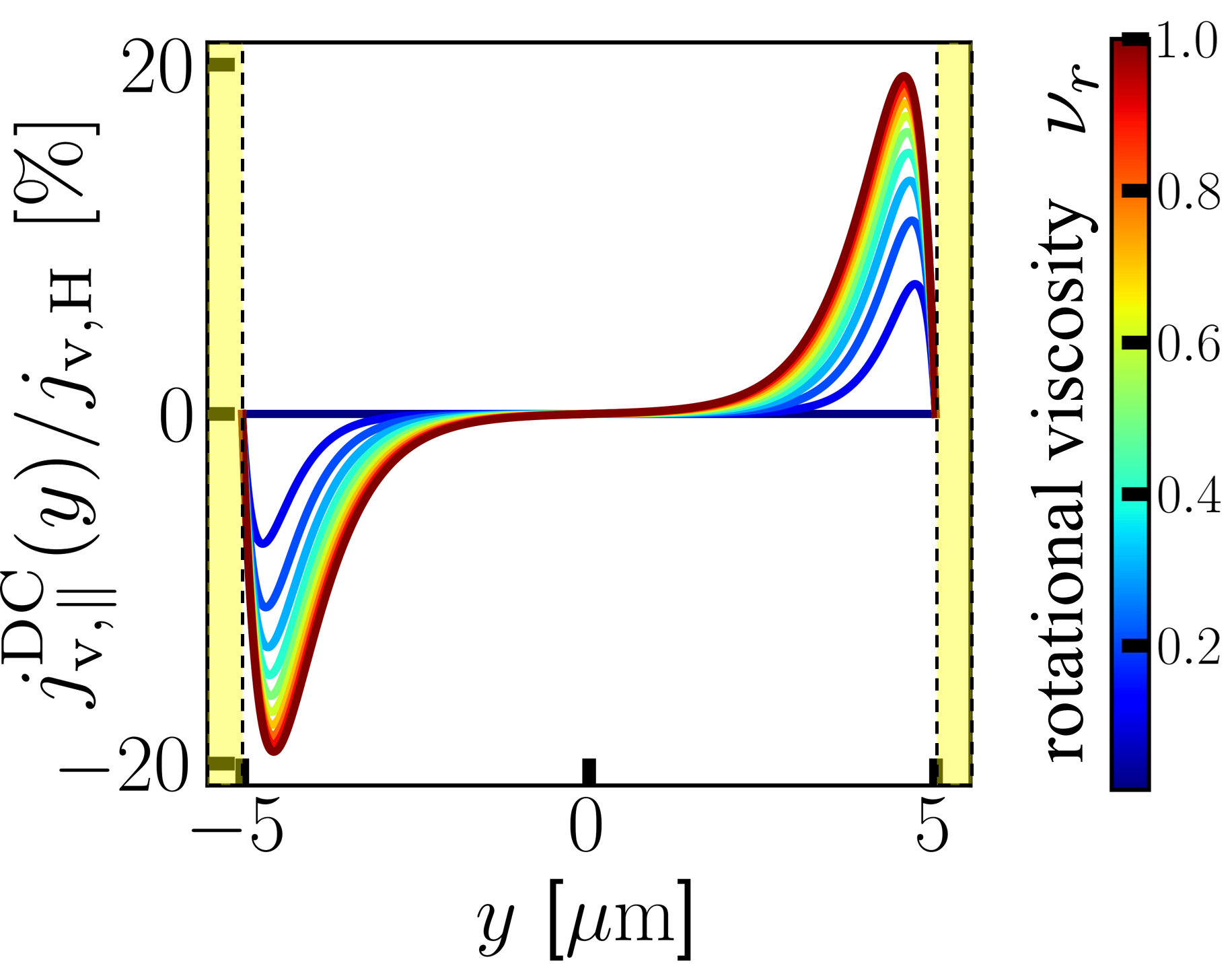
(c) Valley current jv,∥DCj_{\mathrm{v,\parallel}}^{\mathrm{DC}}
Figure 2: (a) Schematics of the valley hydrodynamic generation. In hydrodynamic regime, the valley polarization PvP_{\mathrm{v}} is induced by the microrotation via the valley-microrotation coupling with non-uniform electron velocity 𝒖​(𝒓){\bf\it u}({\bf\it r}), and the longitudinal valley current is generated as 𝒋v=Pv​𝒖{\bf\it j}_{\mathrm{v}}=P_{\mathrm{v}}{\bf\it u}. Plot of (b) the valley polarization and (c) the valley current in the yy-range [−w/2,w/2-w/2,w/2] under DC electric fields for several rotational viscosities. We use the parameters; w=10​μ​mw=10\,\mu\mathrm{m}, E=1×10⁶​Vm−1E=1\times 10^{6}\,\mathrm{Vm^{-1}}, ν=0.1​m2​s−1\nu=0.1\,\mathrm{m^{2}s^{-1}}, I∼10−12​m2I\sim 10^{-12}\,\mathrm{m^{2}}, τR=τvf=1×10⁻¹²​s\tau_{\mathrm{R}}=\tau_{\mathrm{vf}}=1\times 10^{-12}\,\mathrm{s}, a=2.46​Åa=2.46\,\mathrm{\mathring{A}}, t=2.82​eVt=2.82\,\mathrm{eV}, Δ=0.28​eV\Delta=0.28\,\mathrm{eV}, μ=0.15​eV\mu=0.15\,\mathrm{eV}, n=1.4×10¹⁵​m−2n=1.4\times 10^{15}\,\mathrm{m^{-2}}, ρ=2.8×10⁻¹⁷​kgm−2\rho=2.8\times 10^{-17}\,\mathrm{kgm^{-2}}, and the valley Hall current jv,H=2.76×10²¹​m−1​s−1j_{\mathrm{v},\mathrm{H}}=2.76\times 10^{21}\,\mathrm{m^{-1}s^{-1}}.

Valley hydrodynamic generation.— The most significant consequences of our theory is that the interplay between the valley-microrotation coupling and the viscous effects gives rise to an unprecedented longitudinal nonlinear valley current in finite size systems, which has not been addressed so far. We consider the Poiseuille flow in gapped graphene with finite width ww in the yy-direction, which most clearly characterizes the hydrodynamic transport. When we apply DC electric fields in the xx-direction and take no-slip boundary conditions ux(±w/2)=0u_{x}(\pm w/2)=0, the electron fluids form the Poiseuille flow with the velocity profile given by

ux​(y)=−e​n​τRρ​[1−cosh⁡(y/ℓ)cosh⁡(w/2​ℓ)]​E.u_{x}(y)=-\frac{en\tau_{\mathrm{R}}}{\rho}\left[1-\frac{\cosh(y/\ell)}{\cosh(w/2\ell)}\right]E. (17)

The microrotation is also calculated as

ωz​(y)=−τeffτr​12​∂ux∂y=−e​n​τR2​ρ​ℓ​τeffτr​sinh⁡(y/ℓ)cosh⁡(w/2​ℓ)​E,\omega_{z}(y)=-\frac{\tau_{\mathrm{eff}}}{\tau_{r}}\frac{1}{2}\frac{\partial u_{x}}{\partial y}=-\frac{en\tau_{\mathrm{R}}}{2\rho\ell}\frac{\tau_{\mathrm{eff}}}{\tau_{r}}\frac{\sinh(y/\ell)}{\cosh(w/2\ell)}E, (18)

where

ℓ≡(ν+νr​τrτr+τinter)​τR,\ell\equiv\sqrt{\left(\nu+\nu_{r}\frac{\tau_{r}}{\tau_{r}+\tau_{\mathrm{inter}}}\right)\tau_{\mathrm{R}}}, (19)

is a characteristic length that determines the scale of viscous effects. Here, τr−1≡4​νr/I\tau_{r}^{-1}\equiv 4\nu_{r}/I and τeff≡(1/τinter+1/τr)−1\tau_{\mathrm{eff}}\equiv(1/\tau_{\mathrm{inter}}+1/\tau_{r})^{-1} are the rotational and effective relaxation times. From Eq.(9), we obtain the longitudinal valley current profile as [Fig.2(c)]

jv,∥DC(y)=\displaystyle j^{\mathrm{DC}}_{\mathrm{v},\parallel}(y)= (e​n​τRρ​E)2​ℏ​D​(μ)2​ℓ​τeffτr\displaystyle\left(\frac{en\tau_{\mathrm{R}}}{\rho}E\right)^{2}\frac{\hbar D(\mu)}{2\ell}\frac{\tau_{\mathrm{eff}}}{\tau_{r}}
×sinh⁡(y/ℓ)cosh⁡(w/2​ℓ)​[1−cosh⁡(y/ℓ)cosh⁡(w/2​ℓ)].\displaystyle\times\frac{\sinh(y/\ell)}{\cosh(w/2\ell)}\left[1-\frac{\cosh(y/\ell)}{\cosh(w/2\ell)}\right]. (20)

We should note that the rotational viscosity νr\nu_{r} is necessary for realizing a longitudinal nonlinear valley current under DC electric fields. Similar to DC electric fields, an AC electric field along the xx-direction Ex​(t)=Re[E~​e−i​Ω​t]E_{x}(t)=\real[\tilde{E}e^{-i\Omega t}] also induces the Poiseuille flow and leads to the same solutions:

u~x​(y,Ω)=ux​(y)1−i​Ω​τR,ω~z​(y,Ω)=ωz​(y)(1−i​Ω​τeff)​(1−i​Ω​τR),\tilde{u}_{x}(y,\Omega)=\frac{u_{x}(y)}{1-i\Omega\tau_{\mathrm{R}}},\quad\tilde{\omega}_{z}(y,\Omega)=\frac{\omega_{z}(y)}{(1-i\Omega\tau_{\mathrm{eff}})(1-i\Omega\tau_{\mathrm{R}})}, (21)

except for the replacement of ℓ\ell by

ℓ~​(Ω)=(ν+νr​τrτr+τinter​1−i​Ω​τinter1−i​Ω​τeff)​τR1−i​Ω​τR.\tilde{\ell}(\Omega)=\sqrt{\left(\nu+\nu_{r}\frac{\tau_{r}}{\tau_{r}+\tau_{\mathrm{inter}}}\frac{1-i\Omega\tau_{\mathrm{inter}}}{1-i\Omega\tau_{\mathrm{eff}}}\right)\frac{\tau_{\mathrm{R}}}{1-i\Omega\tau_{\mathrm{R}}}}. (22)

Because of the intrinsic nonlinearity of the longitudinal valley current, 𝒋v,∥{\bf\it j}_{\mathrm{v,\parallel}} is composed of the valley counterparts of the rectification and the second harmonic generation:

jv,∥AC(y,t)=jv,∥0(y)+jv,∥2​Ω(y,t).j_{\mathrm{v},\parallel}^{\mathrm{AC}}(y,t)=j_{\mathrm{v},\parallel}^{0}(y)+j_{\mathrm{v},\parallel}^{2\Omega}(y,t). (23)

Circular photovalley generation.— The rotational viscosity-induced valley transport discussed above can be interpreted as a phenomenon of angular momentum conversion between the fluid vorticity and the valley DOF. From this viewpoint, we consider a different scenario for generating a valley polarization by circularly polarized light (CPL). CPL with the electric component 𝑬​(t)=E0​(cos⁡Ω​t,ξ​sin​Ω​t){\bf\it E}(t)=E_{0}(\cos\Omega t,\xi\sin\Omega t) induces a circular motion of electrons, which in turn generates a DC orbital magnetization:

Morbz=−n​e34​m∗2​Ω3​ξ​E02.{M}_{\mathrm{orb}}^{z}=-\frac{ne^{3}}{4{m^{\ast}}^{2}\Omega^{3}}\xi E_{0}^{2}. (24)

This phenomenon is known as the inverse Faraday effect Hertel 2006; Zhang et al. 2009; Battiato et al. 2014; Potashin et al. 2020 owing to the fact that CPL has a spin angular momentum proportional to ξ​E02\xi E_{0}^{2} Barnett and Loudon 2010; Cameron et al. 2012; Bliokh et al. 2013; Bliokh et al. 2014; Bliokh and Nori 2015. Here, the different chirality indices ξ=±1\xi=\pm 1 correspond to the clockwise/counterclockwise circular polarizations. In our hydrodynamic formulation, the orbital magnetization is described as Eq.(16), therefore, the inverse Faraday effect can be regarded as a direct transfer mechanism of angular momentum from CPL to the microrotation.

Refer to caption
Figure 3: Schematics of circular photovalley generation. The microrotation is directly induced by irradiating CPL via the inverse Faraday effect. As a result, a DC valley polarization is generated.

We are now ready to discuss the generation of a valley polarization by CPL dubbed circular photovalley generation [Fig.3]. In contrast to the above discussion, we consider bulk systems with normally-incident CPL. We start from the hydrodynamic equations:

D​𝒖D​t=(ν+νr)Δ𝒖+2νr∇×𝝎−e​n​𝑬ρ−𝒖τR,\displaystyle\frac{D{\bf\it u}}{Dt}=(\nu+\nu_{r})\Delta{\bf\it u}+2\nu_{r}\nabla\times{\bf\it\omega}-\frac{en{\bf\it E}}{\rho}-\frac{{\bf\it u}}{\tau_{\mathrm{R}}}, (25)
D​ωzD​t=1τr​[(∇×𝒖)z2−ωz]−ωzτinter+g​ξ​E02,\displaystyle\frac{D\omega_{z}}{Dt}=\frac{1}{\tau_{r}}\left[\frac{(\nabla\times{\bf\it u})_{z}}{2}-\omega_{z}\right]-\frac{\omega_{z}}{\tau_{\mathrm{inter}}}+g\xi E_{0}^{2}, (26)

where an external angular momentum pumping term stems from the inverse Faraday effect is introduced. By solving Eqs.(S.95a) and (S.95b), the DC component of the microrotation in the second order in electric fields is obtained as

ωz0=τeff​g​ξ​E02,\displaystyle\omega_{z}^{0}=\tau_{\mathrm{eff}}g\xi E_{0}^{2}, (27)

giving rise to a nonlinear DC valley polarization:

Pv0=ℏ​D​(μ)​τeff​g​ξ​E02.\displaystyle P_{\mathrm{v}}^{0}=\hbar D(\mu)\tau_{\mathrm{eff}}g\xi E_{0}^{2}. (28)

Here, the coefficient of gg is estimated as

τeff​g=sgn⁡(μ)​e24​ℏ​a2​t2(ℏ​Ω)3​μ2−Δ2/4Δ2/4,\tau_{\mathrm{eff}}g=\mathrm{sgn}(\mu)\frac{e^{2}}{4\hbar}\frac{a^{2}t^{2}}{(\hbar\Omega)^{3}}\frac{\mu^{2}-\Delta^{2}/4}{\Delta^{2}/4}, (29)

in consistent with Eqs.(16) and (24). In stark contrast to the previous works Cao et al. 2012; Zeng et al. 2012; Mak et al. 2012; Mak and Shan 2016; Ye et al. 2017; Mak et al. 2018, we do not rely on inter-band transition processes, therefore, on-resonant light is not required. This suggests that our hydrodynamic approach broadens the frequency range of CPL and also allows ultrafast manipulation of the valley polarization. This can be achieved by combining the valley DOF with the concept of micropolar fluids. Furthermore, the sign of the valley polarization can be tuned by the chirality ξ\xi of CPL, and hence circular dichroism appears in the valley polarization.

Discussion.—We propose an experimental setup how to determine νr\nu_{r} below. In order to estimate the rotational viscosity experimentally, valley injection provides a reasonable measure. When we inject valley current from the proximity valley Hall materials into valley hydrodynamic materials, the induced valley polarization leads to the non-uniform microrotation profile 𝝎​(𝒓){\bf\it\omega}({\bf\it r}) due to the valley-microrotation coupling. Then, the fluid velocity 𝒖{\bf\it u} is generated by the term νr∇×𝝎\nu_{r}\nabla\times{\bf\it\omega} in Eq.(12). Therefore, we can estimate the rotational viscosity from the observed velocity profile.

Table 1: Comparison of the valley hydrodynamic generation (VHG) and circular photovalley generation (CPVG) as phenomena of angular momentum conversion via valley-microrotation coupling. System, source field, and mechanism are summarized.
VHG CPVG
System Finite size Bulk
Source Electric field Circularly polarized light
Mechanism Rotational viscosity Inverse Faraday effect

Conclusion.—In summary, we have developed a basic framework of valley hydrodynamics in noncentrosymmetric graphene with a staggered sublattice potential, which is composed of the Euler equation Eq.(10) and the balance equation for the microrotation Eq.(11). In addition, we have investigated the interplay between the valley DOF and the microrotation, and elucidated that the valley polarization can be controlled by the microrotation. Our hydrodynamic theory also reveals nonlinear valley dynamics. For example, the rotational viscosity νr\nu_{r} provides a longitudinal nonlinear valley current, which gives rise to the valley counterparts of the rectification and the second harmonic generation. As discussed, νr\nu_{r} can be measured by valley-induced hydrodynamic flow generation. Furthermore, the concept of micropolar fluids sheds light on a rich physics of angular momentum conversion, exemplified by a circular dichroic valley polarization induced by off-resonant light. These results are summarized in Table 1.

The conventional strategy for designing electronic devices in spintronics or valleytronics has been creating confined nanostructure in order to achieve functionality. On the other hand, in hydrodynamic regime, the flow of electrons can become spatially non-uniform due to the viscosities even when the material structure is homogeneous. This suggests a new design guideline for innovative device functionality without nanostructure. Therefore, we believe that the present results provide a building block for future electronics and will pave the way to valleytronic applications of electron hydrodynamics.

Acknowledgements.
The authors are grateful to Yuya Ominato, Shin Kaneshiro, Riki Toshio, Koki Shinada, Hideaki Nishikawa and Hisao Hayakawa for valuable discussions. R.S. thanks Satoshi Kusaba, Kohei Nagai and Kento Uchida for providing helpful comments from an experimental point of view. D.O. is funded by the President’s PhD Scholarships at Imperial College London. This work was supported by the Priority Program of Chinese Academy of Sciences under Grant No. XDB28000000, and by JSPS KAKENHI for Grants (Nos. 20H01863 and 21H04565) from MEXT, Japan.

References

  • Wolf et al. (2001) S. A. Wolf, D. D. Awschalom, R. A. Buhrman, J. M. Daughton, S. von Molnár, M. L. Roukes, A. Y. Chtchelkanova, and D. M. Treger, “Spintronics: A spin-based electronics vision for the future,” Science 294, 1488–1495 (2001).
  • Maekawa et al. (2017) S. Maekawa, S.O. Valenzuela, T. Kimura, and E. Saitoh, Spin Current, Oxford science publications (Oxford University Press, 2017).
  • Xiao et al. (2007) Di Xiao, Wang Yao, and Qian Niu, “Valley-contrasting physics in graphene: Magnetic moment and topological transport,” Phys. Rev. Lett. 99, 236809 (2007).
  • Yao et al. (2008) Wang Yao, Di Xiao, and Qian Niu, “Valley-dependent optoelectronics from inversion symmetry breaking,” Phys. Rev. B 77, 235406 (2008).
  • Xiao et al. (2012) Di Xiao, Gui-Bin Liu, Wanxiang Feng, Xiaodong Xu, and Wang Yao, “Coupled spin and valley physics in monolayers of mos2{\mathrm{mos}}_{2} and other group-vi dichalcogenides,” Phys. Rev. Lett. 108, 196802 (2012).
  • Butler et al. (2013) Sheneve Z. Butler et al., “Progress, challenges, and opportunities in two-dimensional materials beyond graphene,” ACS Nano 7, 2898–2926 (2013).
  • Nguyen and Nguyen (2016) Bich Ha Nguyen and Van Hieu Nguyen, “Two-dimensional hexagonal semiconductors beyond graphene,” Advances in Natural Sciences: Nanoscience and Nanotechnology 7, 043001 (2016).
  • Liu et al. (2017) Fucai Liu, Jiadong Zhou, Chao Zhu, and Zheng Liu, “Electric field effect in two-dimensional transition metal dichalcogenides,” Advanced Functional Materials 27, 1602404 (2017).
  • Choi et al. (2017) Wonbong Choi, Nitin Choudhary, Gang Hee Han, Juhong Park, Deji Akinwande, and Young Hee Lee, “Recent development of two-dimensional transition metal dichalcogenides and their applications,” Materials Today 20, 116–130 (2017).
  • Rycerz et al. (2007) A. Rycerz, J. Tworzydło, and C. W. J. Beenakker, “Valley filter and valley valve in graphene,” Nature Physics 3, 172–175 (2007).
  • Radisavljevic et al. (2011) B. Radisavljevic, A. Radenovic, J. Brivio, V. Giacometti, and A. Kis, “Single-layer mos2 transistors,” Nature Nanotechnology 6, 147–150 (2011).
  • Wang et al. (2012) Qing Hua Wang, Kourosh Kalantar-Zadeh, Andras Kis, Jonathan N. Coleman, and Michael S. Strano, “Electronics and optoelectronics of two-dimensional transition metal dichalcogenides,” Nature Nanotechnology 7, 699–712 (2012).
  • Xu et al. (2014) Xiaodong Xu, Wang Yao, Di Xiao, and Tony F. Heinz, “Spin and pseudospins in layered transition metal dichalcogenides,” Nature Physics 10, 343–350 (2014).
  • Zhang et al. (2014) Y. J. Zhang, T. Oka, R. Suzuki, J. T. Ye, and Y. Iwasa, “Electrically switchable chiral light-emitting transistor,” Science 344, 725–728 (2014).
  • Schaibley et al. (2016) John R. Schaibley, Hongyi Yu, Genevieve Clark, Pasqual Rivera, Jason S. Ross, Kyle L. Seyler, Wang Yao, and Xiaodong Xu, “Valleytronics in 2d materials,” Nature Reviews Materials 1, 16055 (2016).
  • Vitale et al. (2018) Steven A. Vitale, Daniel Nezich, Joseph O. Varghese, Philip Kim, Nuh Gedik, Pablo Jarillo-Herrero, Di Xiao, and Mordechai Rothschild, “Valleytronics: Opportunities, challenges, and paths forward,” Small 14, 1801483 (2018).
  • Liu et al. (2019) Yanping Liu, Yuanji Gao, Siyu Zhang, Jun He, Juan Yu, and Zongwen Liu, “Valleytronics in transition metal dichalcogenides materials,” Nano Research 12, 2695–2711 (2019).
  • Cao et al. (2012) Ting Cao, Gang Wang, Wenpeng Han, Huiqi Ye, Chuanrui Zhu, Junren Shi, Qian Niu, Pingheng Tan, Enge Wang, Baoli Liu, and Ji Feng, “Valley-selective circular dichroism of monolayer molybdenum disulphide,” Nature Communications 3, 887 (2012).
  • Zeng et al. (2012) Hualing Zeng, Junfeng Dai, Wang Yao, Di Xiao, and Xiaodong Cui, “Valley polarization in mos2 monolayers by optical pumping,” Nature Nanotechnology 7, 490–493 (2012).
  • Mak et al. (2012) Kin Fai Mak, Keliang He, Jie Shan, and Tony F. Heinz, “Control of valley polarization in monolayer mos2 by optical helicity,” Nature Nanotechnology 7, 494–498 (2012).
  • Mak and Shan (2016) Kin Fai Mak and Jie Shan, “Photonics and optoelectronics of 2d semiconductor transition metal dichalcogenides,” Nature Photonics 10, 216–226 (2016).
  • Ye et al. (2017) Ziliang Ye, Dezheng Sun, and Tony F. Heinz, “Optical manipulation of valley pseudospin,” Nature Physics 13, 26–29 (2017).
  • Mak et al. (2018) Kin Fai Mak, Di Xiao, and Jie Shan, “Light–valley interactions in 2d semiconductors,” Nature Photonics 12, 451–460 (2018).
  • Li et al. (2014) Yilei Li, Jonathan Ludwig, Tony Low, Alexey Chernikov, Xu Cui, Ghidewon Arefe, Young Duck Kim, Arend M. van der Zande, Albert Rigosi, Heather M. Hill, Suk Hyun Kim, James Hone, Zhiqiang Li, Dmitry Smirnov, and Tony F. Heinz, “Valley splitting and polarization by the zeeman effect in monolayer mose2{\mathrm{mose}}_{2},” Phys. Rev. Lett. 113, 266804 (2014).
  • MacNeill et al. (2015) David MacNeill, Colin Heikes, Kin Fai Mak, Zachary Anderson, Andor Kormányos, Viktor Zólyomi, Jiwoong Park, and Daniel C. Ralph, “Breaking of valley degeneracy by magnetic field in monolayer mose2{\mathrm{mose}}_{2},” Phys. Rev. Lett. 114, 037401 (2015).
  • Srivastava et al. (2015) Ajit Srivastava, Meinrad Sidler, Adrien V. Allain, Dominik S. Lembke, Andras Kis, and A. Imamoğlu, “Valley zeeman effect in elementary optical excitations of monolayer wse2,” Nature Physics 11, 141–147 (2015).
  • Aivazian et al. (2015) G. Aivazian, Zhirui Gong, Aaron M. Jones, Rui-Lin Chu, J. Yan, D. G. Mandrus, Chuanwei Zhang, David Cobden, Wang Yao, and X. Xu, “Magnetic control of valley pseudospin in monolayer wse2,” Nature Physics 11, 148–152 (2015).
  • Back et al. (2017) Patrick Back, Meinrad Sidler, Ovidiu Cotlet, Ajit Srivastava, Naotomo Takemura, Martin Kroner, and Atac Imamoğlu, “Giant paramagnetism-induced valley polarization of electrons in charge-tunable monolayer mose2{\mathrm{mose}}_{2},” Phys. Rev. Lett. 118, 237404 (2017).
  • Mak et al. (2014) K. F. Mak, K. L. McGill, J. Park, and P. L. McEuen, “The valley hall effect in mos2 transistors,” Science 344, 1489–1492 (2014).
  • Gorbachev et al. (2014) R. V. Gorbachev, J. C. W. Song, G. L. Yu, A. V. Kretinin, F. Withers, Y. Cao, A. Mishchenko, I. V. Grigorieva, K. S. Novoselov, L. S. Levitov, and A. K. Geim, “Detecting topological currents in graphene superlattices,” Science 346, 448–451 (2014).
  • Ye et al. (2016) Yu Ye, Jun Xiao, Hailong Wang, Ziliang Ye, Hanyu Zhu, Mervin Zhao, Yuan Wang, Jianhua Zhao, Xiaobo Yin, and Xiang Zhang, “Electrical generation and control of the valley carriers in a monolayer transition metal dichalcogenide,” Nature Nanotechnology 11, 598–602 (2016).
  • Crossno et al. (2016) Jesse Crossno, Jing K. Shi, Ke Wang, Xiaomeng Liu, Achim Harzheim, Andrew Lucas, Subir Sachdev, Philip Kim, Takashi Taniguchi, Kenji Watanabe, Thomas A. Ohki, and Kin Chung Fong, “Observation of the dirac fluid and the breakdown of the wiedemann-franz law in graphene,” Science 351, 1058–1061 (2016).
  • Bandurin et al. (2016) D. A. Bandurin, I. Torre, R. Krishna Kumar, M. Ben Shalom, A. Tomadin, A. Principi, G. H. Auton, E. Khestanova, K. S. Novoselov, I. V. Grigorieva, L. A. Ponomarenko, A. K. Geim, and M. Polini, “Negative local resistance caused by viscous electron backflow in graphene,” Science 351, 1055–1058 (2016).
  • Bandurin et al. (2018) Denis A. Bandurin, Andrey V. Shytov, Leonid S. Levitov, Roshan Krishna Kumar, Alexey I. Berdyugin, Moshe Ben Shalom, Irina V. Grigorieva, Andre K. Geim, and Gregory Falkovich, “Fluidity onset in graphene,” Nature Communications 9, 4533 (2018).
  • Krishna Kumar et al. (2017) R. Krishna Kumar, D. A. Bandurin, F. M. D. Pellegrino, Y. Cao, A. Principi, H. Guo, G. H. Auton, M. Ben Shalom, L. A. Ponomarenko, G. Falkovich, K. Watanabe, T. Taniguchi, I. V. Grigorieva, L. S. Levitov, M. Polini, and A. K. Geim, “Superballistic flow of viscous electron fluid through graphene constrictions,” Nature Physics 13, 1182–1185 (2017).
  • Pellegrino et al. (2017) Francesco M. D. Pellegrino, Iacopo Torre, and Marco Polini, “Nonlocal transport and the hall viscosity of two-dimensional hydrodynamic electron liquids,” Phys. Rev. B 96, 195401 (2017).
  • Berdyugin et al. (2019) A. I. Berdyugin, S. G. Xu, F. M. D. Pellegrino, R. Krishna Kumar, A. Principi, I. Torre, M. Ben Shalom, T. Taniguchi, K. Watanabe, I. V. Grigorieva, M. Polini, A. K. Geim, and D. A. Bandurin, “Measuring hall viscosity of graphene’s electron fluid,” Science 364, 162–165 (2019).
  • Sulpizio et al. (2019) Joseph A. Sulpizio, Lior Ella, Asaf Rozen, John Birkbeck, David J. Perello, Debarghya Dutta, Moshe Ben-Shalom, Takashi Taniguchi, Kenji Watanabe, Tobias Holder, Raquel Queiroz, Alessandro Principi, Ady Stern, Thomas Scaffidi, Andre K. Geim, and Shahal Ilani, “Visualizing poiseuille flow of hydrodynamic electrons,” Nature 576, 75–79 (2019).
  • Gallagher et al. (2019) Patrick Gallagher, Chan-Shan Yang, Tairu Lyu, Fanglin Tian, Rai Kou, Hai Zhang, Kenji Watanabe, Takashi Taniguchi, and Feng Wang, “Quantum-critical conductivity of the dirac fluid in graphene,” Science 364, 158–162 (2019).
  • Polini and Geim (2020) Marco Polini and Andre K. Geim, “Viscous electron fluids,” Physics Today 73, 28–34 (2020).
  • Ku et al. (2020) Mark J. H. Ku, Tony X. Zhou, Qing Li, Young J. Shin, Jing K. Shi, Claire Burch, Laurel E. Anderson, Andrew T. Pierce, Yonglong Xie, Assaf Hamo, Uri Vool, Huiliang Zhang, Francesco Casola, Takashi Taniguchi, Kenji Watanabe, Michael M. Fogler, Philip Kim, Amir Yacoby, and Ronald L. Walsworth, “Imaging viscous flow of the dirac fluid in graphene,” Nature 583, 537–541 (2020).
  • Jenkins et al. (2020) A. Jenkins, S. Baumann, H. Zhou, S. A. Meynell, D. Yang, K. Watanabe, T. Taniguchi, A. Lucas, A. F. Young, and A. C. Bleszynski Jayich, “Imaging the breakdown of ohmic transport in graphene,” (2020), arXiv:2002.05065 [cond-mat.mes-hall] .
  • Geurs et al. (2020) Johannes Geurs, Youngwook Kim, Kenji Watanabe, Takashi Taniguchi, Pilkyung Moon, and Jurgen H. Smet, “Rectification by hydrodynamic flow in an encapsulated graphene tesla valve,” (2020), arXiv:2008.04862 [cond-mat.mes-hall] .
  • Samaddar et al. (2021) Sayanti Samaddar, Jeff Strasdas, Kevin Janßen, Sven Just, Tjorven Johnsen, Zhenxing Wang, Burkay Uzlu, Sha Li, Daniel Neumaier, Marcus Liebmann, and Markus Morgenstern, “Evidence for local spots of viscous electron flow in graphene at moderate mobility,” Nano Letters 21, 9365–9373 (2021).
  • Kumar et al. (2021) Chandan Kumar, John Birkbeck, Joseph A. Sulpizio, David J. Perello, Takashi Taniguchi, Kenji Watanabe, Oren Reuven, Thomas Scaffidi, Ady Stern, Andre K. Geim, and Shahal Ilani, “Imaging hydrodynamic electrons flowing without landauer-sharvin resistance,” (2021), arXiv:2111.06412 [cond-mat.mes-hall] .
  • (46) More detailed discussion is given in the supplemental materials.
  • ERINGEN (1966) A. CEMAL ERINGEN, “Theory of micropolar fluids,” Journal of Mathematics and Mechanics 16, 1–18 (1966).
  • Eringen (1999) A. Cemal Eringen, Microcontinuum Field Theories (Springer New York, 1999).
  • Eringen (2001) A.C. Eringen, Microcontinuum Field Theories: II. Fluent Media, Microcontinuum Field Theories (Springer New York, 2001).
  • Łukaszewicz (1999) Grzegorz Łukaszewicz, Micropolar Fluids (Birkhäuser Boston, 1999).
  • Chandrasekhar et al. (1992) S. Chandrasekhar, P. Morton D Hull Distinguished Service Professor S Chandrasekhar, and Cambridge University Press, Liquid Crystals, Cambridge monographs on physics (Cambridge University Press, 1992).
  • de Gennes and Prost (1993) P.G. de Gennes and J. Prost, The Physics of Liquid Crystals, International Series of Monographs on Physics (Clarendon Press, 1993).
  • Odenbach (2002) Stefan Odenbach, ed., Ferrofluids (Springer Berlin Heidelberg, 2002).
  • Shliomis (1972) Mark Shliomis, “Effective viscosity of magnetic suspensions,” Sov. Phys. JETP 34, 1291–1294 (1972).
  • Rosensweig (2013) R.E. Rosensweig, Ferrohydrodynamics, Dover books on physics (Dover Publications, Incorporated, 2013).
  • Takahashi et al. (2016) R. Takahashi, M. Matsuo, M. Ono, K. Harii, H. Chudo, S. Okayasu, J. Ieda, S. Takahashi, S. Maekawa, and E. Saitoh, “Spin hydrodynamic generation,” Nature Physics 12, 52–56 (2016).
  • Marchetti et al. (2013) M. C. Marchetti, J. F. Joanny, S. Ramaswamy, T. B. Liverpool, J. Prost, Madan Rao, and R. Aditi Simha, “Hydrodynamics of soft active matter,” Rev. Mod. Phys. 85, 1143–1189 (2013).
  • Markovich et al. (2019) Tomer Markovich, Elsen Tjhung, and Michael E Cates, “Chiral active matter: microscopic ‘torque dipoles’ have more than one hydrodynamic description,” New Journal of Physics 21, 112001 (2019).
  • Markovich and Lubensky (2021) Tomer Markovich and Tom C. Lubensky, “Odd viscosity in active matter: Microscopic origin and 3d effects,” Phys. Rev. Lett. 127, 048001 (2021).
  • Shaik and Elfring (2021) Vaseem A Shaik and Gwynn J Elfring, “On the hydrodynamics of active particles in viscosity gradients,” (2021), arXiv:2107.03518 [physics.flu-dyn] .
  • Adamczyk et al. (2017) L. Adamczyk et al., “Global λ\lambda hyperon polarization in nuclear collisions,” Nature 548, 62–65 (2017).
  • Florkowski et al. (2018) Wojciech Florkowski, Bengt Friman, Amaresh Jaiswal, and Enrico Speranza, “Relativistic fluid dynamics with spin,” Phys. Rev. C 97, 041901 (2018).
  • Hattori et al. (2019) Koichi Hattori, Masaru Hongo, Xu-Guang Huang, Mamoru Matsuo, and Hidetoshi Taya, “Fate of spin polarization in a relativistic fluid: An entropy-current analysis,” Physics Letters B 795, 100–106 (2019).
  • Matsuo et al. (2013) Mamoru Matsuo, Jun’ichi Ieda, Kazuya Harii, Eiji Saitoh, and Sadamichi Maekawa, “Mechanical generation of spin current by spin-rotation coupling,” Phys. Rev. B 87, 180402 (2013).
  • Matsuo et al. (2017) M. Matsuo, Y. Ohnuma, and S. Maekawa, “Theory of spin hydrodynamic generation,” Phys. Rev. B 96, 020401 (2017).
  • Kobayashi et al. (2017) D. Kobayashi, T. Yoshikawa, M. Matsuo, R. Iguchi, S. Maekawa, E. Saitoh, and Y. Nozaki, “Spin current generation using a surface acoustic wave generated via spin-rotation coupling,” Phys. Rev. Lett. 119, 077202 (2017).
  • Hughes et al. (2011) Taylor L. Hughes, Robert G. Leigh, and Eduardo Fradkin, “Torsional response and dissipationless viscosity in topological insulators,” Phys. Rev. Lett. 107, 075502 (2011).
  • Xiao et al. (2010) Di Xiao, Ming-Che Chang, and Qian Niu, “Berry phase effects on electronic properties,” Rev. Mod. Phys. 82, 1959–2007 (2010).
  • Lifshitz and Pitaevskii (1981) E. M. Lifshitz and L. P. Pitaevskii, Course of Theoretical Physics: Physical Kinetics (Pergamon, New York, 1981).
  • Lucas and Fong (2018) Andrew Lucas and Kin Chung Fong, “Hydrodynamics of electrons in graphene,” Journal of Physics: Condensed Matter 30, 053001 (2018).
  • Narozhny (2019) Boris N. Narozhny, “Electronic hydrodynamics in graphene,” Annals of Physics 411, 167979 (2019).
  • Narozhny and Schütt (2019) B. N. Narozhny and M. Schütt, “Magnetohydrodynamics in graphene: Shear and hall viscosities,” Phys. Rev. B 100, 035125 (2019).
  • Narozhny and Gornyi (2021) B. N. Narozhny and I. V. Gornyi, “Hydrodynamic approach to electronic transport in graphene: Energy relaxation,” Frontiers in Physics 9, 108 (2021).
  • Kiselev and Schmalian (2020) Egor I. Kiselev and Jörg Schmalian, “Nonlocal hydrodynamic transport and collective excitations in dirac fluids,” Phys. Rev. B 102, 245434 (2020).
  • Berger et al. (2004) Claire Berger, Zhimin Song, Tianbo Li, Xuebin Li, Asmerom Y. Ogbazghi, Rui Feng, Zhenting Dai, Alexei N. Marchenkov, Edward H. Conrad, Phillip N. First, and Walt A. de Heer, “Ultrathin epitaxial graphite:  2d electron gas properties and a route toward graphene-based nanoelectronics,” The Journal of Physical Chemistry B 108, 19912–19916 (2004).
  • Zhou et al. (2007) S. Y. Zhou, G.-H. Gweon, A. V. Fedorov, P. N. First, W. A. de Heer, D.-H. Lee, F. Guinea, A. H. Castro Neto, and A. Lanzara, “Substrate-induced bandgap opening in epitaxial graphene,” Nature Materials 6, 770–775 (2007).
  • Tromp and Hannon (2009) R. M. Tromp and J. B. Hannon, “Thermodynamics and kinetics of graphene growth on sic(0001),” Phys. Rev. Lett. 102, 106104 (2009).
  • Hupalo et al. (2009) M. Hupalo, E. H. Conrad, and M. C. Tringides, “Growth mechanism for epitaxial graphene on vicinal 6​h​-SiC​(0001)6h\text{-SiC}(0001) surfaces: A scanning tunneling microscopy study,” Phys. Rev. B 80, 041401 (2009).
  • Jariwala et al. (2011) Deep Jariwala, Anchal Srivastava, and Pulickel M. Ajayan, “Graphene synthesis and band gap opening,” Journal of Nanoscience and Nanotechnology 11, 6621–6641 (2011).
  • Jeon et al. (2013) Cheolho Jeon, Ha-Chul Shin, Inkyung Song, Minkook Kim, Ji-Hoon Park, Jungho Nam, Dong-Hwa Oh, Sunhee Woo, Chan-Cuk Hwang, Chong-Yun Park, and Joung Real Ahn, “Opening and reversible control of a wide energy gap in uniform monolayer graphene,” Scientific Reports 3, 2725 (2013).
  • Nevius et al. (2015) M. S. Nevius, M. Conrad, F. Wang, A. Celis, M. N. Nair, A. Taleb-Ibrahimi, A. Tejeda, and E. H. Conrad, “Semiconducting graphene from highly ordered substrate interactions,” Phys. Rev. Lett. 115, 136802 (2015).
  • Morozov et al. (2006) S. V. Morozov, K. S. Novoselov, M. I. Katsnelson, F. Schedin, L. A. Ponomarenko, D. Jiang, and A. K. Geim, “Strong suppression of weak localization in graphene,” Phys. Rev. Lett. 97, 016801 (2006).
  • Morpurgo and Guinea (2006) A. F. Morpurgo and F. Guinea, “Intervalley scattering, long-range disorder, and effective time-reversal symmetry breaking in graphene,” Phys. Rev. Lett. 97, 196804 (2006).
  • Gorbachev et al. (2007) R. V. Gorbachev, F. V. Tikhonenko, A. S. Mayorov, D. W. Horsell, and A. K. Savchenko, “Weak localization in bilayer graphene,” Phys. Rev. Lett. 98, 176805 (2007).
  • Sanchez et al. (2016) Oriol Lopez Sanchez, Dmitry Ovchinnikov, Shikhar Misra, Adrien Allain, and Andras Kis, “Valley polarization by spin injection in a light-emitting van der waals heterojunction,” Nano Letters 16, 5792–5797 (2016).
  • Ominato et al. (2021) Yuya Ominato, Daigo Oue, and Mamoru Matsuo, “Valley transport driven by dynamic lattice distortion,” (2021), arXiv:2110.09724 [cond-mat.mes-hall] .
  • Thonhauser (2011) T. Thonhauser, “Theory of orbital magnetization in solids,” International Journal of Modern Physics B 25, 1429–1458 (2011).
  • Kato et al. (2004) Y. K. Kato, R. C. Myers, A. C. Gossard, and D. D. Awschalom, “Observation of the spin hall effect in semiconductors,” Science 306, 1910–1913 (2004).
  • Lee et al. (2016) Jieun Lee, Kin Fai Mak, and Jie Shan, “Electrical control of the valley hall effect in bilayer mos2 transistors,” Nature Nanotechnology 11, 421–425 (2016).
  • Lee et al. (2017) Jieun Lee, Zefang Wang, Hongchao Xie, Kin Fai Mak, and Jie Shan, “Valley magnetoelectricity in single-layer mos2,” Nature Materials 16, 887–891 (2017).
  • Hertel (2006) Riccardo Hertel, “Theory of the inverse faraday effect in metals,” Journal of Magnetism and Magnetic Materials 303, L1–L4 (2006).
  • Zhang et al. (2009) Hui-Liang Zhang, Yan-Zhong Wang, and Xiang-Jun Chen, “A simple explanation for the inverse faraday effect in metals,” Journal of Magnetism and Magnetic Materials 321, L73–L74 (2009).
  • Battiato et al. (2014) M. Battiato, G. Barbalinardo, and P. M. Oppeneer, “Quantum theory of the inverse faraday effect,” Phys. Rev. B 89, 014413 (2014).
  • Potashin et al. (2020) S. O. Potashin, V. Yu. Kachorovskii, and M. S. Shur, “Hydrodynamic inverse faraday effect in a two-dimensional electron liquid,” Phys. Rev. B 102, 085402 (2020).
  • Barnett and Loudon (2010) Stephen M. Barnett and Rodney Loudon, “The enigma of optical momentum in a medium,” Philosophical Transactions of the Royal Society A: Mathematical, Physical and Engineering Sciences 368, 927–939 (2010).
  • Cameron et al. (2012) Robert P Cameron, Stephen M Barnett, and Alison M Yao, “Optical helicity, optical spin and related quantities in electromagnetic theory,” New Journal of Physics 14, 053050 (2012).
  • Bliokh et al. (2013) Konstantin Y Bliokh, Aleksandr Y Bekshaev, and Franco Nori, “Dual electromagnetism: helicity, spin, momentum and angular momentum,” New Journal of Physics 15, 033026 (2013).
  • Bliokh et al. (2014) Konstantin Y Bliokh, Justin Dressel, and Franco Nori, “Conservation of the spin and orbital angular momenta in electromagnetism,” New Journal of Physics 16, 093037 (2014).
  • Bliokh and Nori (2015) Konstantin Y. Bliokh and Franco Nori, “Transverse and longitudinal angular momenta of light,” Physics Reports 592, 1–38 (2015).

Supplemental Materials for
“Valley hydrodynamics in gapped graphene”

I Beyond the Navier-Stokes equation

In this section, we emphasize the need for introducing the concept of micropolar fluids. First, we see the failure of capturing the angular momentum dissipation from the momentum conservation law. In the conventional hydrodynamics, the momentum conservation law leads the well-known Navier-Stokes equation Lifshitz and Pitaevskii 1981:

D​𝒖D​t=ν∇2𝒖−𝒖τR,\frac{D{\bf\it u}}{Dt}=\nu\laplacian{\bf\it u}-\frac{{\bf\it u}}{\tau_{\mathrm{R}}}, (S.1)

where 𝒖{\bf\it u} is the fluid velocity and D/Dt≡∂/∂t+𝒖⋅∇D/Dt\equiv\partial/\partial t+{\bf\it u}\dotproduct\gradient. The dissipation processes of linear momentum are represented by the kinematic viscosity term ν∇2𝒖\nu\laplacian{\bf\it u} and the relaxation term −𝒖/τR-{\bf\it u}/\tau_{\mathrm{R}} in the right-hand side of Eq.(S.1). Here, τR\tau_{\mathrm{R}} is the momentum relaxation time. In order to consider angular momentum flow in the fluid, we take the curl of Eq.(S.1) and obtain an equation for the vorticity 𝜴≡12∇⁣×𝒖{\bf\it\Omega}\equiv\frac{1}{2}\curl{\bf\it u}:

D​𝜴D​t=(𝜴⋅∇)𝒖−ν∇2𝜴−𝜴τR.\frac{D{\bf\it\Omega}}{Dt}=({\bf\it\Omega}\dotproduct\gradient){\bf\it u}-\nu\laplacian{\bf\it\Omega}-\frac{{\bf\it\Omega}}{\tau_{\mathrm{R}}}. (S.2)

Here, we have used the following identity:

(𝒖⋅∇)𝒖=∇12𝒖2−𝒖×(∇⁣×𝒖)=∇12𝒖2−𝒖×2𝜴.({\bf\it u}\dotproduct\gradient){\bf\it u}=\gradient\frac{1}{2}{\bf\it u}^{2}-{\bf\it u}\times(\curl{\bf\it u})=\gradient\frac{1}{2}{\bf\it u}^{2}-{\bf\it u}\times 2{\bf\it\Omega}.

The vorticity equation Eq.(S.2) is merely a mathematical transformation of Eq.(S.1); therefore, Eq.(S.2) does not contain the information of dissipation processes of angular momentum.

In order to take the angular momentum dissipation into account, we go back to the fundamental level of the conservation laws. Let us consider angular momentum conservation by introducing the normal stress 𝒕n{\bf\it t}_{n} as well as the body torque 𝒍{\bf\it l} and the couple stress 𝝀n{\bf\it\lambda}_{n}:

ddt⁡∫V⁡(t)ρ⁡[𝒓×𝒖+𝒔]=∫∂V⁡(t)(𝒓×𝒕n+𝝀n)+∫V⁡(t)(𝒓×ρ​𝒃+ρ​𝒍),\derivative{t}\int_{V(t)}\rho[{\bf\it r}\times{\bf\it u}+{\bf\it s}]=\int_{\partial V(t)}({\bf\it r}\times{\bf\it t}_{n}+{\bf\it\lambda}_{n})+\int_{V(t)}({\bf\it r}\times\rho{\bf\it b}+\rho{\bf\it l}), (S.3)

where ρ\rho is the mass density, 𝒔{\bf\it s} is the internal angular momentum per unit fluid mass, 𝒃{\bf\it b} is the body force, V⁡(t)V(t) is the element of volume, and ∂V⁡(t)\partial V(t) is the surface of the volume. By using the relations 𝒕n=𝒏⋅𝐓{\bf\it t}_{n}={\bf\it n}\dotproduct\mathbf{T} and 𝝀n=𝒏⋅𝚲{\bf\it\lambda}_{n}={\bf\it n}\dotproduct\mathbf{\Lambda}, the right-hand side of Eq.(S.3) reads

∫V⁡(t)(𝒓×ρ​𝒃+ρ​𝒍+∇⁣⋅⁡𝚲+𝒓×(∇⁣⋅⁡𝐓)+𝐓x),\int_{V(t)}({\bf\it r}\times\rho{\bf\it b}+\rho{\bf\it l}+\divergence\mathbf{\Lambda}+{\bf\it r}\times(\divergence\mathbf{T})+\mathbf{T}_{x}), (S.4)

where 𝚲\mathbf{\Lambda} is the couple stress tensor and (𝐓x)i=ϵi​j​k​Tj​k(\mathbf{T}_{x})_{i}=\epsilon_{ijk}T_{jk} is the axial vector component of the stress tensor 𝐓\mathbf{T}. From Eqs.(S.3) and (S.4), we obtain

ρ​𝒓×(D​𝒖D​t−∇⁣⋅⁡𝐓−𝒃)+D​𝒔D​t=ρ​𝒍+∇⁣⋅⁡𝚲+𝐓x,\rho{\bf\it r}\times\left(\frac{D{\bf\it u}}{Dt}-\divergence\mathbf{T}-{\bf\it b}\right)+\frac{D{\bf\it s}}{Dt}=\rho{\bf\it l}+\divergence\mathbf{\Lambda}+\mathbf{T}_{x}, (S.5)

where the bracket in the left-hand side is the momentum conservation law Lifshitz and Pitaevskii 1981:

ddt⁡∫V⁡(t)ρ​𝒖=∫∂V⁡(t)𝒕n+∫V⁡(t)ρ​𝒃,\derivative{t}\int_{V(t)}\rho{\bf\it u}=\int_{\partial V(t)}{\bf\it t}_{n}+\int_{V(t)}\rho{\bf\it b}, (S.6)

and hence vanishes. In the following, we consider isotropic micropolar fluids, whose internal angular momentum density can be described as

ρ​𝒔=ρ​I​𝝎,\rho{\bf\it s}=\rho I{\bf\it\omega}, (S.7)

where II is the microinertia per unit fluid mass and 𝝎{\bf\it\omega} is the internal rotation of the fluid elements. Combining Eqs.(S.5)-(S.7), we obtain the equation for the internal angular momentum:

ρ​I​D​𝝎D​t=ρ​𝒍+∇⁣⋅⁡𝚲+𝐓x.\rho I\frac{D{\bf\it\omega}}{Dt}=\rho{\bf\it l}+\divergence\mathbf{\Lambda}+\mathbf{T}_{x}. (S.8)

Note that the stress tensor in the conventional hydrodynamics is restricted to be symmetric: 𝐓=𝐓s\mathbf{T}=\mathbf{T}^{\mathrm{s}}, therefore, 𝐓x\mathbf{T}_{x} is absent. This corresponds to the fact that the conventional hydrodynamics focuses only on linear momentum conservation while disregards angular momentum conservation. Thus, the antisymmetric components of the stress tensor play a crucial role in dissipation processes of angular momentum.

Following the standard approach of micropolar fluids Eringen 1999, we assume that the antisymmetric components of the stress tensor 𝐓a\mathbf{T}^{\mathrm{a}} are given by

(𝐓a)i​j=μr​(∂iuj−∂jui)−2​μr​ϵi​j​k​ωk,(\mathbf{T}^{\mathrm{a}})_{ij}=\mu_{r}(\partial_{i}u_{j}-\partial_{j}u_{i})-2\mu_{r}\epsilon_{ijk}\omega_{k}, (S.9)

with the rotational viscosity μr\mu_{r}. In the most simple case, the couple stress tensor and the body torque are absent, 𝚲=𝒍=0\mathbf{\Lambda}={\bf\it l}=0, we obtain the simplified equation for angular momentum:

ρ​I​D​𝝎D​t=4​μr​(𝜴−𝝎),\rho I\frac{D{\bf\it\omega}}{Dt}=4\mu_{r}({\bf\it\Omega}-{\bf\it\omega}), (S.10)

which includes dissipation processes of angular momentum between the vorticity and the microrotation.

II Formulation

In this section, we outline how to derive the valley hydrodynamic equations for noncentrosymmetric graphene with a staggered sublattice potential, which are correct up to the second order in electric fields. We start from the Boltzmann equation,

∂fα​τ∂t+𝒓˙α​τ⋅∂fα​τ∂𝒓+𝒌˙α​τ⋅∂fα​τ∂𝒌=−fα​τ−fα​τNτN−fα​τ−f0τR−fα​τ−fα−ττvf,\partialderivative{f_{\alpha\tau}}{t}+\dot{{\bf\it r}}_{\alpha\tau}\dotproduct\partialderivative{f_{\alpha\tau}}{\vb*{r}}+\dot{{\bf\it k}}_{\alpha\tau}\dotproduct\partialderivative{f_{\alpha\tau}}{\vb*{k}}=-\frac{f_{\alpha\tau}-f_{\alpha\tau}^{\mathrm{N}}}{\tau_{\mathrm{N}}}-\frac{f_{\alpha\tau}-f_{0}}{\tau_{\mathrm{R}}}-\frac{f_{\alpha\tau}-f_{\alpha-\tau}}{\tau_{\mathrm{vf}}}, (S.11)

where τN\tau_{\mathrm{N}}, τR\tau_{\mathrm{R}} and τvf\tau_{\mathrm{vf}} are the relaxation times for normal (N), resistive (R), and valley flipping processes. τN\tau_{\mathrm{N}} and τvf\tau_{\mathrm{vf}} stem from normal electron-electron scatterings and these processes conserve the linear momentum. On the other hand, τR\tau_{\mathrm{R}} stems from Umklapp scatterings, impurity scatterings, and electron-phonon scatterings, therefore, this process does not conserve the linear momentum. The difference between N and valley flipping processes is that the former conserve the valley polarization, while the latter does not. fα​τ​(𝒓,𝒌,t)f_{\alpha\tau}({\bf\it r},{\bf\it k},t) is the distribution function of an electron with band α\alpha and valley τ\tau. The semiclassical equations of motion read Xiao et al. 2010

𝒓˙α​τ=1ℏ​∂ϵα​τ​(𝒌)∂𝒌−𝒌˙α​τ×𝜴α​τ,𝒌˙α​τ=−eℏ​𝑬,\dot{{\bf\it r}}_{\alpha\tau}=\frac{1}{\hbar}\partialderivative{\epsilon_{\alpha\tau}(\vb*{k})}{\vb*{k}}-\dot{{\bf\it k}}_{\alpha\tau}\times{\bf\it\Omega}_{\alpha\tau},\quad\dot{{\bf\it k}}_{\alpha\tau}=-\frac{e}{\hbar}{\bf\it E}, (S.12)

where the electric field 𝑬{\bf\it E} is independent of position for simplicity. A more detailed explanation of other physical variables is given in the main text.

Following the standard approach Lifshitz and Pitaevskii 1981; Lucas and Fong 2018, the continuity equations for the charge carrier density and the linear momentum are obtained in the relaxation-time approximation as follows:

∂n∂t+∇⁣⋅⁡𝒋=0,\displaystyle\partialderivative{n}{t}+\divergence{\bf\it j}=0, (S.13)
∂Pi∂t+∂Πi​j∂xj=−e​n​Ei−PiτR,\displaystyle\partialderivative{P_{i}}{t}+\partialderivative{\Pi_{ij}}{x_j}=-enE_{i}-\frac{P_{i}}{\tau_{\mathrm{R}}}, (S.14)

where nn and 𝑷{\bf\it P} are the particle density and the momentum of electrons, −e​n​𝑬-en{\bf\it E} is the driving force due to external electric fields and τR\tau_{\mathrm{R}} is the relaxation-time for momentum-relaxing scatterings. In Eqs. (S.13) and (S.14), 𝒋n{\bf\it j}_{n} and Πi​j\Pi_{ij} are the corresponding fluxes of each density. In the following, we will show the detailed derivation of Eqs. (S.13) and (S.14).

III law of conservation of particle number

First, integrating the Boltzmann equation (S.11) over the momentum space, we obtain the following equation:

∑α,τ∫[d𝒌]​∂fα​τ∂t+∑α,τ∫[d𝒌]​𝒓˙α​τ⋅∂fα​τ∂𝒓+∑α,τ∫[d𝒌]​𝒌˙α​τ⋅∂fα​τ∂𝒌\displaystyle\sum_{\alpha,\tau}\int[\differential{\vb*{k}}]\partialderivative{f_{\alpha\tau}}{t}+\sum_{\alpha,\tau}\int[\differential{\vb*{k}}]\dot{{\bf\it r}}_{\alpha\tau}\dotproduct\partialderivative{f_{\alpha\tau}}{\vb*{r}}+\sum_{\alpha,\tau}\int[\differential{\vb*{k}}]\dot{{\bf\it k}}_{\alpha\tau}\dotproduct\partialderivative{f_{\alpha\tau}}{\vb*{k}}
=−∑α,τ∫[d𝒌]fα​τ−fα​τNτN−∑α,τ∫[d𝒌]fα​τ−f0τR−∑α,τ∫[d𝒌]fα​τ−fα−ττvf.\displaystyle\quad=-\sum_{\alpha,\tau}\int[\differential{\vb*{k}}]\frac{f_{\alpha\tau}-f_{\alpha\tau}^{\mathrm{N}}}{\tau_{\mathrm{N}}}-\sum_{\alpha,\tau}\int[\differential{\vb*{k}}]\frac{f_{\alpha\tau}-f_{0}}{\tau_{\mathrm{R}}}-\sum_{\alpha,\tau}\int[\differential{\vb*{k}}]\frac{f_{\alpha\tau}-f_{\alpha-\tau}}{\tau_{\mathrm{vf}}}. (S.15)

In the following, we calculate each term respectively. The only subtle point arising in two-band systems is the treatment of the formally infinite number of particles in the filled band. In other words, we need to make a distinction between the “particle density" and “carrier density". However, assuming the contribution of the filled band to be constant, we can immediately see that it vanishes upon differentiation and does not contribute to the continuity equations. Integrating by parts the first term on the left-hand side of (S.15), we obtain the expression of the charge density nn,

∑α,τ∫[d𝒌]​∂fα​τ∂t=∂∂t⁡∑τ∫[d𝒌]​[f+,τ−(1−f−,τ)]=∂∂t⁡(n+−n−)≡∂n∂t.\sum_{\alpha,\tau}\int[\differential{\vb*{k}}]\partialderivative{f_{\alpha\tau}}{t}=\partialderivative{t}\sum_{\tau}\int[\differential{\vb*{k}}][f_{+,\tau}-(1-f_{-,\tau})]=\partialderivative{t}(n_+-n_{-})\equiv\partialderivative{n}{t}. (S.16)

The definitions of the numbers of charge carriers in the two bands, n±n_{\pm}, are given by

n+\displaystyle n_{+} ≡∑τ∫[d𝒌]​f+,τ,\displaystyle\equiv\sum_{\tau}\int[\differential{\vb*{k}}]f_{+,\tau}, (S.17a)
n−\displaystyle n_{-} ≡∑τ∫[d𝒌]​(1−f−,τ),\displaystyle\equiv\sum_{\tau}\int[\differential{\vb*{k}}](1-f_{-,\tau}), (S.17b)
with the total carrier density being
n=n+−n−.n=n_{+}-n_{-}. (S.17c)
Summing up the densities (S.17a) and (S.17b), we may define the “imbalance" or the total quasiparticle density
nI≡n++n−.n_{I}\equiv n_{+}+n_{-}. (S.17d)

Performing similar procedures for the second and third terms on the left-hand side of Eq. (S.15), we obtain

∑α,τ∫[d𝒌]​𝒓˙α​τ⋅∂fα​τ∂𝒓\displaystyle\sum_{\alpha,\tau}\int[\differential{\vb*{k}}]\dot{{\bf\it r}}_{\alpha\tau}\dotproduct\partialderivative{f_{\alpha\tau}}{\vb*{r}} =∇⁣⋅∑τ∫[d𝒌][𝒓˙+,τf+,τ−𝒓˙−,τ(1−f−,τ)]\displaystyle=\divergence\sum_{\tau}\int[\differential{\vb*{k}}][\dot{{\bf\it r}}_{+,\tau}f_{+,\tau}-\dot{{\bf\it r}}_{-,\tau}(1-f_{-,\tau})]
=∇⋅(𝒋+−𝒋−)≡∇⁣⋅⁡𝒋,\displaystyle=\divergence(\vb*{j}_+-\vb*{j}_{-})\equiv\divergence{\bf\it j}, (S.18)

defining the electric current 𝒋{\bf\it j} and the quasiparticle currents 𝒋±{\bf\it j}_{\pm}:

𝒋\displaystyle{\bf\it j} ≡𝒋+−𝒋−,\displaystyle\equiv{\bf\it j}_{+}-{\bf\it j}_{-}, (S.19a)
𝒋+\displaystyle{\bf\it j}_{+} =∑τ∫[d𝒌]​(1ℏ​∂ϵ+,τ​(𝒌)∂𝒌+eℏ​𝑬×𝜴+,τ​(𝒌))​f+,τ,\displaystyle=\sum_{\tau}\int[\differential{\vb*{k}}]\left(\frac{1}{\hbar}\partialderivative{\epsilon_{+,\tau}(\vb*{k})}{\vb*{k}}+\frac{e}{\hbar}{\bf\it E}\times{\bf\it\Omega}_{+,\tau}({\bf\it k})\right)f_{+,\tau}, (S.19b)
𝒋−\displaystyle{\bf\it j}_{-} =∑τ∫[d𝒌]​(1ℏ​∂ϵ−,τ​(𝒌)∂𝒌+eℏ​𝑬×𝜴−,τ​(𝒌))​(1−f−,τ),\displaystyle=\sum_{\tau}\int[\differential{\vb*{k}}]\left(\frac{1}{\hbar}\partialderivative{\epsilon_{-,\tau}(\vb*{k})}{\vb*{k}}+\frac{e}{\hbar}{\bf\it E}\times{\bf\it\Omega}_{-,\tau}({\bf\it k})\right)(1-f_{-,\tau}), (S.19c)

and

∑α,τ∫[d𝒌]​𝒌˙α​τ⋅∂fα​τ∂𝒌\displaystyle\sum_{\alpha,\tau}\int[\differential{\vb*{k}}]\dot{{\bf\it k}}_{\alpha\tau}\dotproduct\partialderivative{f_{\alpha\tau}}{\vb*{k}} =−eℏ𝑬⋅∑α,τ∫[d𝒌]∂fα​τ∂𝒌=−eℏ𝑬⋅∑τ∫[d𝒌][∂f+,τ∂𝒌−∂∂𝒌⁡(1−f−,τ)]=0.\displaystyle=-\frac{e}{\hbar}{\bf\it E}\dotproduct\sum_{\alpha,\tau}\int[\differential{\vb*{k}}]\partialderivative{f_{\alpha\tau}}{\vb*{k}}=-\frac{e}{\hbar}{\bf\it E}\dotproduct\sum_{\tau}\int[\differential{\vb*{k}}]\left[\partialderivative{f_{+,\tau}}{\vb*{k}}-\partialderivative{\vb*{k}}(1-f_{-,\tau})\right]=0. (S.20)

For the physical reasons that the total number of carriers does not change due to scatterings, we conclude that each term on the right-hand side of Eq. (S.15) should vanish:

∑α,τ∫[d𝒌]​fα​τ−fα​τNτN=∑α,τ∫[d𝒌]​fα​τ−f0τR=∑α,τ∫[d𝒌]​fα​τ−fα−ττvf=0.\sum_{\alpha,\tau}\int[\differential{\vb*{k}}]\frac{f_{\alpha\tau}-f_{\alpha\tau}^{\mathrm{N}}}{\tau_{\mathrm{N}}}=\sum_{\alpha,\tau}\int[\differential{\vb*{k}}]\frac{f_{\alpha\tau}-f_{0}}{\tau_{\mathrm{R}}}=\sum_{\alpha,\tau}\int[\differential{\vb*{k}}]\frac{f_{\alpha\tau}-f_{\alpha-\tau}}{\tau_{\mathrm{vf}}}=0. (S.21)

Summarizing the above equations (S.15)-(S.21), we obtain the continuity equation (S.13),

∂n∂t+∇⁣⋅⁡𝒋=0.\partialderivative{n}{t}+\divergence{\bf\it j}=0. (S.22)

Multiplying the Boltzmann equation by α\alpha and integrating over all states, we can find a similar continuity equation for the imbalance density,

∂nI∂t+∇⁣⋅⁡𝒋I=0,\partialderivative{n_I}{t}+\divergence{\bf\it j}_{I}=0, (S.23)

with the imbalance current,

𝒋I≡𝒋++𝒋−.{\bf\it j}_{I}\equiv{\bf\it j}_{+}+{\bf\it j}_{-}. (S.24)

Note that we have not considered the recombination processes, which do not conserve the number of particles in each band individually. Therefore, the imbalance density is also conserved.

IV Balance Equation of Linear Momentum

The momentum conserving law is obtained by multiplying the Boltzmann equation (S.11) with ℏ​ki\hbar k_{i} and integrating over the momentum space:

∑α,τ∫[d𝒌]​ℏ​ki​∂fα​τ∂t+∑α,τ∫[d𝒌]​ℏ​ki​𝒓˙α​τ⋅∂fα​τ∂𝒓+∑α,τ∫[d𝒌]​ℏ​ki​𝒌˙α​τ⋅∂fα​τ∂𝒌\displaystyle\sum_{\alpha,\tau}\int[\differential{\vb*{k}}]\hbar k_{i}\partialderivative{f_{\alpha\tau}}{t}+\sum_{\alpha,\tau}\int[\differential{\vb*{k}}]\hbar k_{i}\dot{{\bf\it r}}_{\alpha\tau}\dotproduct\partialderivative{f_{\alpha\tau}}{\vb*{r}}+\sum_{\alpha,\tau}\int[\differential{\vb*{k}}]\hbar k_{i}\dot{{\bf\it k}}_{\alpha\tau}\dotproduct\partialderivative{f_{\alpha\tau}}{\vb*{k}}
=−∑α,τ∫[d𝒌]ℏkifα​τ−fα​τNτN−∑α,τ∫[d𝒌]ℏkifα​τ−f0τR−∑α,τ∫[d𝒌]ℏkifα​τ−fα−ττvf.\displaystyle\quad=-\sum_{\alpha,\tau}\int[\differential{\vb*{k}}]\hbar k_{i}\frac{f_{\alpha\tau}-f_{\alpha\tau}^{\mathrm{N}}}{\tau_{\mathrm{N}}}-\sum_{\alpha,\tau}\int[\differential{\vb*{k}}]\hbar k_{i}\frac{f_{\alpha\tau}-f_{0}}{\tau_{\mathrm{R}}}-\sum_{\alpha,\tau}\int[\differential{\vb*{k}}]\hbar k_{i}\frac{f_{\alpha\tau}-f_{\alpha-\tau}}{\tau_{\mathrm{vf}}}. (S.25)

Here and hereafter, the Einstein summation convention is implied for repeated indices. Each term on the left-hand side of Eq. (S.25) is calculated by taking similar procedures with particle conservation law:

∑α,τ∫[d𝒌]​ℏ​ki​∂fα​τ∂t\displaystyle\sum_{\alpha,\tau}\int[\differential{\vb*{k}}]\hbar k_{i}\partialderivative{f_{\alpha\tau}}{t} =∂∂t⁡∑α,τ∫[d𝒌]​ℏ​ki​fα​τ=∂Pi∂t,\displaystyle=\partialderivative{t}\sum_{\alpha,\tau}\int[\differential{\vb*{k}}]\hbar k_{i}f_{\alpha\tau}=\partialderivative{P_i}{t}, (S.26)
∑α,τ∫[d𝒌]​ℏ​ki​r˙n​τ,j​∂fα​τ∂xj\displaystyle\sum_{\alpha,\tau}\int[\differential{\vb*{k}}]\hbar k_{i}\dot{r}_{n\tau,j}\partialderivative{f_{\alpha\tau}}{x_j} =∑α,τ∫[d𝒌]​ki​(∂ϵα​τ​(𝒌)∂kj+e​ϵj​k​l​Ek​Ωn​τ,l)​∂fα​τ∂xj\displaystyle=\sum_{\alpha,\tau}\int[\differential{\vb*{k}}]k_{i}\left(\partialderivative{\epsilon_{\alpha\tau}(\vb*{k})}{k_j}+e\epsilon_{jkl}E_{k}\Omega_{n\tau,l}\right)\partialderivative{f_{\alpha\tau}}{x_j}
=∂∂xj⁡∑α,τ∫[d𝒌]​ki​(∂ϵα​τ​(𝒌)∂kj+e​ϵj​k​l​Ek​Ωn​τ,l)​fα​τ=∂Πi​j∂xj,\displaystyle=\partialderivative{x_j}\sum_{\alpha,\tau}\int[\differential{\vb*{k}}]k_{i}\left(\partialderivative{\epsilon_{\alpha\tau}(\vb*{k})}{k_j}+e\epsilon_{jkl}E_{k}\Omega_{n\tau,l}\right)f_{\alpha\tau}=\partialderivative{\Pi_{ij}}{x_j}, (S.27)
∑α,τ∫[d𝒌]​ℏ​ki​k˙n​τ,j​∂fα​τ∂kj\displaystyle\sum_{\alpha,\tau}\int[\differential{\vb*{k}}]\hbar k_{i}\dot{k}_{n\tau,j}\partialderivative{f_{\alpha\tau}}{k_j} =−eEj∑τ∫[d𝒌]ki∂∂kj[f+,τ−(1−f−,τ)]\displaystyle=-eE_{j}\sum_{\tau}\int[\differential{\vb*{k}}]k_{i}\partialderivative{k_j}[f_{+,\tau}-(1-f_{-,\tau})]
=e​Ei​∑τ∫[d𝒌]​[f+,τ−(1−f−,τ)]=e​n​Ei,\displaystyle=eE_{i}\sum_{\tau}\int[\differential{\vb*{k}}][f_{+,\tau}-(1-f_{-,\tau})]=enE_{i}, (S.28)

where we have defined the total momentum PiP_{i} and the momentum flux Πi​j\Pi_{ij} as follows:

Pi\displaystyle P_{i} =∑α,τ∫[d𝒌]​ℏ​ki​fα​τ,\displaystyle=\sum_{\alpha,\tau}\int[\differential{\vb*{k}}]\hbar k_{i}f_{\alpha\tau}, (S.29)
Πi​j\displaystyle\Pi_{ij} =∑α,τ∫[d𝒌]​ki​(∂ϵα​τ​(𝒌)∂kj+e​ϵj​k​l​Ek​Ωn​τ,l)​fα​τ.\displaystyle=\sum_{\alpha,\tau}\int[\differential{\vb*{k}}]k_{i}\left(\partialderivative{\epsilon_{\alpha\tau}(\vb*{k})}{k_j}+e\epsilon_{jkl}E_{k}\Omega_{n\tau,l}\right)f_{\alpha\tau}. (S.30)

On the other hand, each term on the right-hand side of Eq. (S.25) is calculated as follows:

−∑α,τ∫[d𝒌]ℏkifα​τ−fα​τNτN\displaystyle-\sum_{\alpha,\tau}\int[\differential{\vb*{k}}]\hbar k_{i}\frac{f_{\alpha\tau}-f_{\alpha\tau}^{\mathrm{N}}}{\tau_{\mathrm{N}}} =−1τN​(∑α,τ∫[d𝒌]​ℏ​ki​fα​τ−∑α,τ∫[d𝒌]​ℏ​ki​fα​τN)=0,\displaystyle=-\frac{1}{\tau_{\mathrm{N}}}\left(\sum_{\alpha,\tau}\int[\differential{\vb*{k}}]\hbar k_{i}f_{\alpha\tau}-\sum_{\alpha,\tau}\int[\differential{\vb*{k}}]\hbar k_{i}f_{\alpha\tau}^{\mathrm{N}}\right)=0, (S.31)
−∑α,τ∫[d𝒌]ℏkifα​τ−f0τR\displaystyle-\sum_{\alpha,\tau}\int[\differential{\vb*{k}}]\hbar k_{i}\frac{f_{\alpha\tau}-f_{0}}{\tau_{\mathrm{R}}} =−1τR​(∑α,τ∫[d𝒌]​ℏ​ki​fα​τ−∑α,τ∫[d𝒌]​ℏ​ki​f0)=−PiτR,\displaystyle=-\frac{1}{\tau_{\mathrm{R}}}\left(\sum_{\alpha,\tau}\int[\differential{\vb*{k}}]\hbar k_{i}f_{\alpha\tau}-\sum_{\alpha,\tau}\int[\differential{\vb*{k}}]\hbar k_{i}f_{0}\right)=-\frac{P_{i}}{\tau_{\mathrm{R}}}, (S.32)
−∑α,τ∫[d𝒌]ℏkifα​τ−fα−ττvf\displaystyle-\sum_{\alpha,\tau}\int[\differential{\vb*{k}}]\hbar k_{i}\frac{f_{\alpha\tau}-f_{\alpha-\tau}}{\tau_{\mathrm{vf}}} =−1τvf​(∑α,τ∫[d𝒌]​ℏ​ki​fα​τ−∑α,τ∫[d𝒌]​ℏ​ki​fα−τ)\displaystyle=-\frac{1}{\tau_{\mathrm{vf}}}\left(\sum_{\alpha,\tau}\int[\differential{\vb*{k}}]\hbar k_{i}f_{\alpha\tau}-\sum_{\alpha,\tau}\int[\differential{\vb*{k}}]\hbar k_{i}f_{\alpha-\tau}\right)
=−1τvf​(∑α,τ∫[d𝒌]​ℏ​ki​fα​τ−∑α,τ∫[d𝒌]​ℏ​ki​fα​τ)=0.\displaystyle=-\frac{1}{\tau_{\mathrm{vf}}}\left(\sum_{\alpha,\tau}\int[\differential{\vb*{k}}]\hbar k_{i}f_{\alpha\tau}-\sum_{\alpha,\tau}\int[\differential{\vb*{k}}]\hbar k_{i}f_{\alpha\tau}\right)=0. (S.33)

Here, we have used the features of the local equilibrium distribution function fα​τNf_{\alpha\tau}^{\mathrm{N}} and the global equilibrium distribution function f0f_{0}:

∑α,τ∫[d𝒌]​ℏ​ki​fα​τ=∑α,τ∫[d𝒌]​ℏ​ki​fα​τN,\displaystyle\sum_{\alpha,\tau}\int[\differential{\vb*{k}}]\hbar k_{i}f_{\alpha\tau}=\sum_{\alpha,\tau}\int[\differential{\vb*{k}}]\hbar k_{i}f_{\alpha\tau}^{\mathrm{N}}, (S.34)
∑α,τ∫[d𝒌]​ℏ​ki​f0=0.\displaystyle\sum_{\alpha,\tau}\int[\differential{\vb*{k}}]\hbar k_{i}f_{0}=0. (S.35)

After all, PiP_{i} and Πi​j\Pi_{ij} satisfy the momentum conservation law (S.14),

∂Pi∂t+∂Πi​j∂xj=−e​n​Ei−PiτR\partialderivative{P_i}{t}+\partialderivative{\Pi_{ij}}{x_j}=-enE_{i}-\frac{P_{i}}{\tau_{\mathrm{R}}} (S.36)

with the driving force −e​n​Ei-enE_{i} and the momentum-relaxing force −Pi/τR-P_{i}/\tau_{\mathrm{R}}.

V Balance Equation of Valley polarization

A necessary requirement for valleytronics applications is the ability to generate and control the valley polarization. Analogous to the spin polarization, we define the valley polarization as a population imbalance between two valleys:

Pv​(𝒓,t)=∑αnα,+K−∑αnα,−K=∑α,ττ​∫[d𝒌]​fα​τ​(𝒓,𝒌,t).P_{\mathrm{v}}({\bf\it r},t)=\sum_{\alpha}n_{\alpha,+K}-\sum_{\alpha}n_{\alpha,-K}=\sum_{\alpha,\tau}\tau\int[\differential{\vb*{k}}]f_{\alpha\tau}({\bf\it r},{\bf\it k},t). (S.37)

In the systems we consider, an emergent conservation law appears owing to large separation of two valleys in momentum space. The valley conservation law is obtained by multiplying the Boltzmann equation (S.11) with valley index τ\tau and integrating over the momentum space:

∑α,ττ​∫[d𝒌]​∂fα​τ∂t+∑α,ττ​∫[d𝒌]​𝒓˙α​τ⋅∂fα​τ∂𝒓+∑α,ττ​∫[d𝒌]​𝒌˙α​τ⋅∂fα​τ∂𝒌\displaystyle\sum_{\alpha,\tau}\tau\int[\differential{\vb*{k}}]\partialderivative{f_{\alpha\tau}}{t}+\sum_{\alpha,\tau}\tau\int[\differential{\vb*{k}}]\dot{{\bf\it r}}_{\alpha\tau}\dotproduct\partialderivative{f_{\alpha\tau}}{\vb*{r}}+\sum_{\alpha,\tau}\tau\int[\differential{\vb*{k}}]\dot{{\bf\it k}}_{\alpha\tau}\dotproduct\partialderivative{f_{\alpha\tau}}{\vb*{k}}
=−∑α,ττ∫[d𝒌]fα​τ−fα​τNτN−∑α,ττ∫[d𝒌]fα​τ−f0τR−∑α,ττ∫[d𝒌]fα​τ−fα−ττvf.\displaystyle\quad=-\sum_{\alpha,\tau}\tau\int[\differential{\vb*{k}}]\frac{f_{\alpha\tau}-f_{\alpha\tau}^{\mathrm{N}}}{\tau_{\mathrm{N}}}-\sum_{\alpha,\tau}\tau\int[\differential{\vb*{k}}]\frac{f_{\alpha\tau}-f_{0}}{\tau_{\mathrm{R}}}-\sum_{\alpha,\tau}\tau\int[\differential{\vb*{k}}]\frac{f_{\alpha\tau}-f_{\alpha-\tau}}{\tau_{\mathrm{vf}}}. (S.38)

Each term on the left-hand side of Eq. (S.38) is calculated by taking similar procedures with particle conservation law:

∑α,ττ​∫[d𝒌]​∂fα​τ∂t\displaystyle\sum_{\alpha,\tau}\tau\int[\differential{\vb*{k}}]\partialderivative{f_{\alpha\tau}}{t} =∂∂t⁡∑α,ττ​∫[d𝒌]​fα​τ=∂Pv∂t,\displaystyle=\partialderivative{t}\sum_{\alpha,\tau}\tau\int[\differential{\vb*{k}}]f_{\alpha\tau}=\partialderivative{P_{\mathrm{v}}}{t}, (S.39)
∑α,ττ​∫[d𝒌]​𝒓˙α​τ⋅∂fα​τ∂𝒓\displaystyle\sum_{\alpha,\tau}\tau\int[\differential{\vb*{k}}]\dot{{\bf\it r}}_{\alpha\tau}\dotproduct\partialderivative{f_{\alpha\tau}}{\vb*{r}} =∑α,ττ​∫[d𝒌]​(1ℏ​∂ϵα​τ​(𝒌)∂𝒌+eℏ​𝑬×𝜴α​τ​(𝒌))⋅∂fα​τ∂𝒓\displaystyle=\sum_{\alpha,\tau}\tau\int[\differential{\vb*{k}}]\left(\frac{1}{\hbar}\partialderivative{\epsilon_{\alpha\tau}(\vb*{k})}{\vb*{k}}+\frac{e}{\hbar}{\bf\it E}\times{\bf\it\Omega}_{\alpha\tau}({\bf\it k})\right)\dotproduct\partialderivative{f_{\alpha\tau}}{\vb*{r}}
=∇⁣⋅∑α,ττ∫[d𝒌](1ℏ∂ϵα​τ​(𝒌)∂𝒌+eℏ𝑬×𝜴α​τ(𝒌))fα​τ\displaystyle=\divergence\sum_{\alpha,\tau}\tau\int[\differential{\vb*{k}}]\left(\frac{1}{\hbar}\partialderivative{\epsilon_{\alpha\tau}(\vb*{k})}{\vb*{k}}+\frac{e}{\hbar}{\bf\it E}\times{\bf\it\Omega}_{\alpha\tau}({\bf\it k})\right)f_{\alpha\tau}
=∇⁣⋅⁡𝒋v,\displaystyle=\divergence{\bf\it j}_{\mathrm{v}}, (S.40)
∑α,ττ​∫[d𝒌]​𝒌˙α​τ⋅∂fα​τ∂𝒌\displaystyle\sum_{\alpha,\tau}\tau\int[\differential{\vb*{k}}]\dot{{\bf\it k}}_{\alpha\tau}\dotproduct\partialderivative{f_{\alpha\tau}}{\vb*{k}} =eℏ​𝑬⋅∑α,ττ​∫[d𝒌]​∂∂𝒌⁡[f+,τ−(1−f−,τ)]=0.\displaystyle=\frac{e}{\hbar}{\bf\it E}\dotproduct\sum_{\alpha,\tau}\tau\int[\differential{\vb*{k}}]\partialderivative{\vb*{k}}[f_{+,\tau}-(1-f_{-,\tau})]=0. (S.41)

Here, we have defined the valley polarization PvP_{\mathrm{v}} and the valley current 𝒋v{\bf\it j}_{\mathrm{v}} as follows:

Pv\displaystyle P_{\mathrm{v}} =∑α,ττ​∫[d𝒌]​fα​τ,\displaystyle=\sum_{\alpha,\tau}\tau\int[\differential{\vb*{k}}]f_{\alpha\tau}, (S.42)
𝒋v\displaystyle{\bf\it j}_{\mathrm{v}} =∑α,ττ​∫[d𝒌]​(1ℏ​∂ϵα​τ​(𝒌)∂𝒌+eℏ​𝑬×𝜴α​τ​(𝒌))​fα​τ.\displaystyle=\sum_{\alpha,\tau}\tau\int[\differential{\vb*{k}}]\left(\frac{1}{\hbar}\partialderivative{\epsilon_{\alpha\tau}(\vb*{k})}{\vb*{k}}+\frac{e}{\hbar}{\bf\it E}\times{\bf\it\Omega}_{\alpha\tau}({\bf\it k})\right)f_{\alpha\tau}. (S.43)

On the other hand, each term on the right-hand side of Eq. (S.38) is calculated as follows:

−∑α,ττ∫[d𝒌]fα​τ−fα​τNτN\displaystyle-\sum_{\alpha,\tau}\tau\int[\differential{\vb*{k}}]\frac{f_{\alpha\tau}-f_{\alpha\tau}^{\mathrm{N}}}{\tau_{\mathrm{N}}} =−1τN​(∑α,ττ​∫[d𝒌]​fα​τ−∑α,ττ​∫[d𝒌]​fα​τN)=0,\displaystyle=-\frac{1}{\tau_{\mathrm{N}}}\left(\sum_{\alpha,\tau}\tau\int[\differential{\vb*{k}}]f_{\alpha\tau}-\sum_{\alpha,\tau}\tau\int[\differential{\vb*{k}}]f_{\alpha\tau}^{\mathrm{N}}\right)=0, (S.44)
−∑α,ττ∫[d𝒌]fα​τ−f0τR\displaystyle-\sum_{\alpha,\tau}\tau\int[\differential{\vb*{k}}]\frac{f_{\alpha\tau}-f_{0}}{\tau_{\mathrm{R}}} =−1τR​(∑α,ττ​∫[d𝒌]​fα​τ−∑α,ττ​∫[d𝒌]​f0)=−PvτR,\displaystyle=-\frac{1}{\tau_{\mathrm{R}}}\left(\sum_{\alpha,\tau}\tau\int[\differential{\vb*{k}}]f_{\alpha\tau}-\sum_{\alpha,\tau}\tau\int[\differential{\vb*{k}}]f_{0}\right)=-\frac{P_{\mathrm{v}}}{\tau_{\mathrm{R}}}, (S.45)
−∑α,ττ∫[d𝒌]fα​τ−fα−ττvf\displaystyle-\sum_{\alpha,\tau}\tau\int[\differential{\vb*{k}}]\frac{f_{\alpha\tau}-f_{\alpha-\tau}}{\tau_{\mathrm{vf}}} =−1τvf​(∑α,ττ​∫[d𝒌]​fα​τ−∑α,ττ​∫[d𝒌]​fα−τ)\displaystyle=-\frac{1}{\tau_{\mathrm{vf}}}\left(\sum_{\alpha,\tau}\tau\int[\differential{\vb*{k}}]f_{\alpha\tau}-\sum_{\alpha,\tau}\tau\int[\differential{\vb*{k}}]f_{\alpha-\tau}\right)
=−1τvf​(∑α,ττ​∫[d𝒌]​fα​τ+∑α,τ(−τ)​∫[d𝒌]​fα−τ)\displaystyle=-\frac{1}{\tau_{\mathrm{vf}}}\left(\sum_{\alpha,\tau}\tau\int[\differential{\vb*{k}}]f_{\alpha\tau}+\sum_{\alpha,\tau}(-\tau)\int[\differential{\vb*{k}}]f_{\alpha-\tau}\right)
=−1τvf​(∑α,ττ​∫[d𝒌]​fα​τ+∑α,ττ​∫[d𝒌]​fα​τ)=−2​Pvτvf.\displaystyle=-\frac{1}{\tau_{\mathrm{vf}}}\left(\sum_{\alpha,\tau}\tau\int[\differential{\vb*{k}}]f_{\alpha\tau}+\sum_{\alpha,\tau}\tau\int[\differential{\vb*{k}}]f_{\alpha\tau}\right)=-\frac{2P_{\mathrm{v}}}{\tau_{\mathrm{vf}}}. (S.46)

Here, we have used the features of the local distribution function fα​τNf_{\alpha\tau}^{\mathrm{N}} and the global equilibrium distribution function f0f_{0}:

∑α,ττ​∫[d𝒌]​fα​τ=∑α,ττ​∫[d𝒌]​fα​τN,\displaystyle\sum_{\alpha,\tau}\tau\int[\differential{\vb*{k}}]f_{\alpha\tau}=\sum_{\alpha,\tau}\tau\int[\differential{\vb*{k}}]f_{\alpha\tau}^{\mathrm{N}}, (S.47)
∑α,ττ​∫[d𝒌]​f0=0,\displaystyle\sum_{\alpha,\tau}\tau\int[\differential{\vb*{k}}]f_{0}=0, (S.48)

where the second equation claims the valley polarization is absent in equilibrium. After all, PvP_{\mathrm{v}} and 𝒋v{\bf\it j}_{\mathrm{v}} satisfy the valley conservation law,

∂Pv∂t+∇⁣⋅⁡𝒋v=−PvτR−2​Pvτvf.\partialderivative{P_{\mathrm{v}}}{t}+\divergence{\bf\it j}_{\mathrm{v}}=-\frac{P_{\mathrm{v}}}{\tau_{\mathrm{R}}}-\frac{2P_{\mathrm{v}}}{\tau_{\mathrm{vf}}}. (S.49)

VI Summary of continuity equations

To summarize, we list all four continuity equations for two-band electronic systems as follows,

∂n∂t+∇⁣⋅⁡𝒋=0,\displaystyle\partialderivative{n}{t}+\divergence{\bf\it j}=0, (S.50a)
∂nI∂t+∇⁣⋅⁡𝒋I=0,\displaystyle\partialderivative{n_I}{t}+\divergence{\bf\it j}_{I}=0, (S.50b)
∂Pi∂t+∂Πi​j∂xj=−e​n​Ei−PiτR,\displaystyle\partialderivative{P_i}{t}+\partialderivative{\Pi_{ij}}{x_j}=-enE_{i}-\frac{P_{i}}{\tau_{\mathrm{R}}}, (S.50c)
∂Pv∂t+∇⁣⋅⁡𝒋v=−PvτR−2​Pvτvf.\displaystyle\partialderivative{P_\mathrm{v}}{t}+\divergence{\bf\it j}_{\mathrm{v}}=-\frac{P_{\mathrm{v}}}{\tau_{\mathrm{R}}}-\frac{2P_{\mathrm{v}}}{\tau_{\mathrm{vf}}}. (S.50d)

VII local equilibrium distribution function

From the above discussions, independent conserved quantities (n,nI,𝑷rel,Pv)(n,n_{I},{\bf\it P}_{\mathrm{rel}},P_{\mathrm{v}}) are obtained as follows.

n⁡(𝒓,t)\displaystyle n({\bf\it r},t) =∑α,τ∫[d𝒌]​fα​τ,\displaystyle=\sum_{\alpha,\tau}\int[\differential{\bf\it k}]f_{\alpha\tau}, (S.51)
nI​(𝒓,t)\displaystyle n_{I}({\bf\it r},t) =∑α,τα​∫[d𝒌]​fα​τ,\displaystyle=\sum_{\alpha,\tau}\alpha\int[\differential{\bf\it k}]f_{\alpha\tau}, (S.52)
𝑷​(𝒓,t)\displaystyle{\bf\it P}({\bf\it r},t) =∑α,τ∫[d𝒌]​ℏ​(𝒌+𝑲τ)​fα​τ=∑α,τ∫[d𝒌]​ℏ​𝒌​fα​τ+ℏ​𝑲​∑α,ττ​∫[d𝒌]​fα​τ,\displaystyle=\sum_{\alpha,\tau}\int[\differential{\bf\it k}]\hbar({\bf\it k}+{\bf\it K}_{\tau})f_{\alpha\tau}=\sum_{\alpha,\tau}\int[\differential{\bf\it k}]\hbar{\bf\it k}f_{\alpha\tau}+\hbar{\bf\it K}\sum_{\alpha,\tau}\tau\int[\differential{\bf\it k}]f_{\alpha\tau},
=𝑷rel+ℏ​𝑲​Pv,\displaystyle={\bf\it P}_{\mathrm{rel}}+\hbar{\bf\it K}P_{\mathrm{v}}, (S.53)
Pv​(𝒓,t)\displaystyle P_{\mathrm{v}}({\bf\it r},t) =∑α,ττ​∫[d𝒌]​fα​τ,\displaystyle=\sum_{\alpha,\tau}\tau\int[\differential{\bf\it k}]f_{\alpha\tau}, (S.54)

with the energy and entropy densities,

E⁡(𝒓,t)\displaystyle E({\bf\it r},t) =∑α,τ∫[d𝒌]​ϵα​τ​(𝒌)​fα​τ,\displaystyle=\sum_{\alpha,\tau}\int[\differential{\bf\it k}]\epsilon_{\alpha\tau}({\bf\it k})f_{\alpha\tau}, (S.55)
S⁡(𝒓,t)\displaystyle S({\bf\it r},t) =−kB∑α,τ∫[d𝒌]{fα​τlogfα​τ+(1−fα​τ)log⁡(1−fα​τ)}.\displaystyle=-k_{\mathrm{B}}\sum_{\alpha,\tau}\int[\differential{\bf\it k}]\Bigl\{f_{\alpha\tau}\log f_{\alpha\tau}+(1-f_{\alpha\tau})\log(1-f_{\alpha\tau})\Bigr\}. (S.56)

Here, we introduce the free energy which is a functional of non-equilibrium distribution function fα​τf_{\alpha\tau} with corresponding parameters (μ,μI,𝒖,ωz)(\mu,\mu_{I},{\bf\it u},\omega_{z}) for conserved quantities (n,nI,𝑷rel,Pv)(n,n_{I},{\bf\it P}_{\mathrm{rel}},P_{\mathrm{v}}),

Ω⁡[fα​τ]\displaystyle\Omega[f_{\alpha\tau}] =E−T​S−μ​n−𝒖⋅𝑷rel−ℏ​ωz​Pv\displaystyle=E-TS-\mu n-{\bf\it u}\dotproduct{\bf\it P}_{\mathrm{rel}}-\hbar\omega_{z}P_{\mathrm{v}}
=∑α​τ∫[d𝒌]​[{ϵα​τ​(𝒌)−μ−α​μI−𝒖⋅ℏ​𝒌−ℏ​ωz​τ}​fα​τ+kB​T​{fα​τ​log⁡fα​τ+(1−fα​τ)​log⁡(1−fα​τ)}].\displaystyle=\sum_{\alpha\tau}\int[\differential{\bf\it k}]\biggl[\Bigl\{\epsilon_{\alpha\tau}({\bf\it k})-\mu-\alpha\mu_{I}-{\bf\it u}\dotproduct\hbar{\bf\it k}-\hbar\omega_{z}\tau\Bigr\}f_{\alpha\tau}+k_{\mathrm{B}}T\Bigl\{f_{\alpha\tau}\log f_{\alpha\tau}+(1-f_{\alpha\tau})\log(1-f_{\alpha\tau})\Bigr\}\biggr]. (S.57)

The local equilibrium distribution function is obtained by the variational principle for the functional Ω⁡[fα​τ]\Omega[f_{\alpha\tau}],

δ​Ωδ​fα​τ|fα​τ=fα​τN=ϵα​τ​(𝒌)−μ−α​μI−𝒖⋅ℏ​𝒌−ℏ​ωz​τ+kB​T​log⁡fα​τN1−fα​τN=0.\left.\frac{\delta\Omega}{\delta f_{\alpha\tau}}\right|_{f_{\alpha\tau}=f_{\alpha\tau}^{\mathrm{N}}}=\epsilon_{\alpha\tau}({\bf\it k})-\mu-\alpha\mu_{I}-{\bf\it u}\dotproduct\hbar{\bf\it k}-\hbar\omega_{z}\tau+k_{\mathrm{B}}T\log\frac{f_{\alpha\tau}^{\mathrm{N}}}{1-f_{\alpha\tau}^{\mathrm{N}}}=0. (S.58)

In this end, we obtain the local equilibrium distribution function:

fα​τN=[1+exp⁡{ϵα​τ−ℏ​𝒌⋅𝒖−ℏ​ωz​τ−μαkB​T}]−1,f_{\alpha\tau}^{\mathrm{N}}=\left[1+\exp\left\{\frac{\epsilon_{\alpha\tau}-\hbar{\bf\it k}\dotproduct{\bf\it u}-\hbar\omega_{z}\tau-\mu_{\alpha}}{k_{\mathrm{B}}T}\right\}\right]^{-1}, (S.59)

where μα≡μ+α​μI\mu_{\alpha}\equiv\mu+\alpha\mu_{I} is the local chemical potential, 𝒖{\bf\it u} is the hydrodynamic velocity, and ωz\omega_{z} is the microrotation. In the following analysis, we assume that μI=0\mu_{I}=0 for simplicity. In global equilibrium, the distribution function is given by

f0​(𝒌)=fα​τN​(𝒌)|μI=0,𝒖=0,ωz=0.f_{0}({\bf\it k})=f_{\alpha\tau}^{\mathrm{N}}({\bf\it k})|_{\mu_{I}=0,{\bf\it u}=0,\omega_{z}=0}. (S.60)

VIII model hamiltonian

In order to use the local distribution function Eq.(S.59) in practical calculations, we need to specify the quasiparticle spectrum. A monolayer graphene with a staggered sublatice potential breaking the inversion symmetry is a concrete example for considering valley hydrodynamics. The effective Hamiltonian describing electron states in the vicinity of the KK and −K-K points is given by

Hτ=a​t​(τ​kx​σx+ky​σy)+Δ2​σz.H_{\tau}=at(\tau k_{x}\sigma_{x}+k_{y}\sigma_{y})+\frac{\Delta}{2}\sigma_{z}. (S.61)

A detailed explanation of parameters is given in the main text. The energy eigenvalues are obtained as

ϵα​τ​(𝒌)=α​Δ2/4+(a​t​k)2.\epsilon_{\alpha\tau}({\bf\it k})=\alpha\sqrt{\Delta^{2}/4+(atk)^{2}}. (S.62)

From these energy eigenvalues, we can calculate the density of states as follows,

D⁡(ϵ)=∑α,τ∫[d𝐤]​δ​[ϵ−ϵα​τ​(𝒌)]=|ϵ|π​a2​t2​θ​(ϵ2−Δ2/4).D(\epsilon)=\sum_{\alpha,\tau}\int[\differential\mathbf{k}]\delta[\epsilon-\epsilon_{\alpha\tau}({\bf\it k})]=\frac{\absolutevalue{\epsilon}}{\pi a^{2}t^{2}}\theta(\epsilon^{2}-\Delta^{2}/4). (S.63)

Using the energy eigenfunctions, we also obtain the Berry curvature

Ωα​τz​(𝒌)=−2​α​τ​Δ(Δ2+4​a2​t2​k2)3/2.\Omega^{z}_{\alpha\tau}({\bf\it k})=-2\alpha\tau\frac{\Delta}{(\Delta^{2}+4a^{2}t^{2}k^{2})^{3/2}}. (S.64)

The orbital magnetic moment is one of the valley contrasting parameters in 2D materials. In gapped graphene, the orbital magnetic moment is given by

𝔪α​τz​(𝒌)=−τ​e2​ℏ​2​a2​t2​ΔΔ2+4​a2​t2​k2=eℏ​ϵα​τ​(𝒌)​Ωα​τz​(𝒌),\mathfrak{m}_{\alpha\tau}^{z}({\bf\it k})=-\tau\frac{e}{2\hbar}\frac{2a^{2}t^{2}\Delta}{\Delta^{2}+4a^{2}t^{2}k^{2}}=\frac{e}{\hbar}\epsilon_{\alpha\tau}({\bf\it k})\Omega^{z}_{\alpha\tau}({\bf\it k}), (S.65)

which can be intuitively interpreted as the self-rotation of the Bloch wave packet.

IX hydrodynamic variables

In order to construct the effective hydrodynamic theory, which is correct up to first order in the velocity and the microrotation, we introduce several concepts. In hydrodynamic regime, the system reaches to local equilibrium via normal electron-electron scatterings which conserve the linear momentum and the valley polarization. For this reason, we can assume that the distribution functions are approximately described as the local equilibrium distribution function:

fα​τ≃fα​τN=[1+exp⁡{ϵα​τ−ℏ​𝒌⋅𝒖−ℏ​ωz​τ−μkB​T}]−1.f_{\alpha\tau}\simeq f_{\alpha\tau}^{\mathrm{N}}=\left[1+\exp\left\{\frac{\epsilon_{\alpha\tau}-\hbar{\bf\it k}\dotproduct{\bf\it u}-\hbar\omega_{z}\tau-\mu}{k_{\mathrm{B}}T}\right\}\right]^{-1}. (S.66)

From now on, we assume that the band energy has an isotropic parabolic dispersion with the same effective mass m∗=ℏ2​Δ/2​a2​t2m^{\ast}=\hbar^{2}\Delta/2a^{2}t^{2} around some valleys: ϵα​τ=α⁡[Δ/2+𝒑2/2​m∗]\epsilon_{\alpha\tau}=\alpha[\Delta/2+{\bf\it p}^{2}/2m^{\ast}], where 𝒑{\bf\it p} is defined as a deviation from the valley. This assumption is reasonable since the relevant conduction and valence bands for noncentrosymmetric graphene with a staggered sublattice potential are well described by Eq.(S.61). We also assume that the underlying effective theory is invariant under Galilean transformation: fα​τN​(𝒑+α​m∗​𝒖)=f0​(ϵα​τ​(𝒑))f_{\alpha\tau}^{\mathrm{N}}({\bf\it p}+\alpha m^{\ast}{\bf\it u})=f_{0}(\epsilon_{\alpha\tau}({\bf\it p})) for an free-like dispersion ϵα​τ​(𝒑)=α⁡[Δ/2+𝒑2/2​m∗]\epsilon_{\alpha\tau}({\bf\it p})=\alpha[\Delta/2+{\bf\it p}^{2}/2m^{\ast}].

IX.1 I. Law of Conservation of particle number

We are now ready to express three conservation laws in terms of hydrodynamic variables. First, the quasiparticle densities n±n_{\pm} can be expressed as follows:

n+\displaystyle n_{+} =∑τ∫[d𝒌]​f+,τN​(𝒌)=∑τ∫[d𝒑]​f+,τN​(𝒑+m+∗​𝒖)=∑τ∫[d𝒌]​f0​(ϵ+,τ​(𝒌)−ℏ​τ​ωz)\displaystyle=\sum_{\tau}\int[\differential{\vb*{k}}]f_{+,\tau}^{\mathrm{N}}({\bf\it k})=\sum_{\tau}\int[\differential{\vb*{p}}]f_{+,\tau}^{\mathrm{N}}({\bf\it p}+m^{\ast}_{+}{\bf\it u})=\sum_{\tau}\int[\differential{\vb*{k}}]f_{0}(\epsilon_{+,\tau}({\bf\it k})-\hbar\tau\omega_{z})
=∑τ∫[d𝒌]​f0​(ϵ+,τ​(𝒌))+ℏ​ωz​∑ττ​∫[d𝒌]​(−∂f0​(ϵ+,τ​(𝒌))∂ϵ)\displaystyle=\sum_{\tau}\int[\differential{\vb*{k}}]f_{0}(\epsilon_{+,\tau}({\bf\it k}))+\hbar\omega_{z}\sum_{\tau}\tau\int[\differential{\vb*{k}}]\left(-\partialderivative{f_0(\epsilon_{+,\tau}(\vb*{k}))}{\epsilon}\right)
=∑τ∫[d𝒌]​f0​(ϵ+,τ​(𝒌)),\displaystyle=\sum_{\tau}\int[\differential{\vb*{k}}]f_{0}(\epsilon_{+,\tau}({\bf\it k})), (S.67a)
n−\displaystyle n_{-} =∑τ∫[d𝒌]​[1−f−,τN​(𝒌)]=∑τ∫[d𝒑]​[1−f−,τN​(𝒑+m−∗​𝒖)]=∑τ∫[d𝒌]​[1−f0​(ϵ−,τ​(𝒌)−ℏ​τ​ωz)]\displaystyle=\sum_{\tau}\int[\differential{\vb*{k}}][1-f_{-,\tau}^{\mathrm{N}}({\bf\it k})]=\sum_{\tau}\int[\differential{\vb*{p}}][1-f_{-,\tau}^{\mathrm{N}}({\bf\it p}+m^{\ast}_{-}{\bf\it u})]=\sum_{\tau}\int[\differential{\vb*{k}}][1-f_{0}(\epsilon_{-,\tau}({\bf\it k})-\hbar\tau\omega_{z})]
=∑τ∫[d𝒌]​[1−f0​(ϵ−,τ​(𝒌))]−ℏ​ωz​(𝒓,t)​∑α,ττ​∫[d𝒌]​(−∂f0​(ϵ−,τ​(𝒌))∂ϵ)\displaystyle=\sum_{\tau}\int[\differential{\vb*{k}}][1-f_{0}(\epsilon_{-,\tau}({\bf\it k}))]-\hbar\omega_{z}({\bf\it r},t)\sum_{\alpha,\tau}\tau\int[\differential{\vb*{k}}]\left(-\partialderivative{f_0(\epsilon_{-,\tau}(\vb*{k}))}{\epsilon}\right)
=∑τ∫[d𝒌]​[1−f0​(ϵ−,τ​(𝒌))],\displaystyle=\sum_{\tau}\int[\differential{\vb*{k}}][1-f_{0}(\epsilon_{-,\tau}({\bf\it k}))], (S.67b)
where we have used the fact that the band energy ϵα​τ​(𝒌)\epsilon_{\alpha\tau}({\bf\it k}) does not depend on τ\tau. From these calculations, we obtain the charge carrier and the imbalance densities as follows:
n\displaystyle n =n+−n−=∑τ∫[d𝒌]​[f0​(ϵ+,τ​(𝒌))−{1−f0​(ϵ−,τ​(𝒌))}],\displaystyle=n_{+}-n_{-}=\sum_{\tau}\int[\differential{\vb*{k}}][f_{0}(\epsilon_{+,\tau}({\bf\it k}))-\{1-f_{0}(\epsilon_{-,\tau}({\bf\it k}))\}], (S.67c)
nI\displaystyle n_{I} =n++n−=∑τ∫[d𝒌]​[f0​(ϵ+,τ​(𝒌))+{1−f0​(ϵ−,τ​(𝒌))}].\displaystyle=n_{+}+n_{-}=\sum_{\tau}\int[\differential{\vb*{k}}][f_{0}(\epsilon_{+,\tau}({\bf\it k}))+\{1-f_{0}(\epsilon_{-,\tau}({\bf\it k}))\}]. (S.67d)

The same calculations can be performed for the quasiparticle currents,

𝒋+\displaystyle{\bf\it j}_{+} =∑τ∫[d𝒌]​(1ℏ​∂ϵ+,τ​(𝒌)∂𝒌+eℏ​𝑬×𝜴+,τ​(𝒑))​f+,τN​(𝒌)\displaystyle=\sum_{\tau}\int[\differential{\vb*{k}}]\left(\frac{1}{\hbar}\partialderivative{\epsilon_{+,\tau}(\vb*{k})}{\vb*{k}}+\frac{e}{\hbar}{\bf\it E}\times{\bf\it\Omega}_{+,\tau}({\bf\it p})\right)f_{+,\tau}^{\mathrm{N}}({\bf\it k})
=∑τ∫[d𝒑]​(𝒑+m+∗​𝒖m+∗+eℏ​𝑬×𝜴+,τ​(𝒑+m+∗​𝒖))​f+,τN​(𝒑+m+∗​𝒖)⏟f0​(ϵ+,τ−ℏ​ωz​τ)\displaystyle=\sum_{\tau}\int[\differential{\vb*{p}}]\left(\frac{{\bf\it p}+m^{\ast}_{+}{\bf\it u}}{m^{\ast}_{+}}+\frac{e}{\hbar}{\bf\it E}\times{\bf\it\Omega}_{+,\tau}({\bf\it p}+m^{\ast}_{+}{\bf\it u})\right)\underbrace{f_{+,\tau}^{\mathrm{N}}({\bf\it p}+m^{\ast}_{+}{\bf\it u})}_{f_{0}(\epsilon_{+,\tau}-\hbar\omega_{z}\tau)}
=n+​𝒖+e​ℏ​ωz​𝑬×∑ττ​∫[d𝒑]​Ω+,τ​(−∂f0​(ϵ+,τ)∂ϵ),\displaystyle=n_{+}{\bf\it u}+e\hbar\omega_{z}{\bf\it E}\times\sum_{\tau}\tau\int[\differential{\bf\it p}]\Omega_{+,\tau}\left(-\partialderivative{f_0(\epsilon_{+,\tau})}{\epsilon}\right), (S.68a)
𝒋−\displaystyle{\bf\it j}_{-} =∑τ∫[d𝒌]​(1ℏ​∂ϵ−,τ​(𝒌)∂𝒌+eℏ​𝑬×𝜴−,τ​(𝒑))​[1−f−,τN​(𝒌)]\displaystyle=\sum_{\tau}\int[\differential{\vb*{k}}]\left(\frac{1}{\hbar}\partialderivative{\epsilon_{-,\tau}(\vb*{k})}{\vb*{k}}+\frac{e}{\hbar}{\bf\it E}\times{\bf\it\Omega}_{-,\tau}({\bf\it p})\right)[1-f_{-,\tau}^{\mathrm{N}}({\bf\it k})]
=∑τ∫[d𝒑]​(𝒑+m−∗​𝒖m−∗+eℏ​𝑬×𝜴−,τ​(𝒑+m−∗​𝒖))​[1−f−,τN​(𝒑+m−∗​𝒖)⏟f0​(ϵ−,τ−ℏ​ωz​τ)]\displaystyle=\sum_{\tau}\int[\differential{\vb*{p}}]\left(\frac{{\bf\it p}+m^{\ast}_{-}{\bf\it u}}{m^{\ast}_{-}}+\frac{e}{\hbar}{\bf\it E}\times{\bf\it\Omega}_{-,\tau}({\bf\it p}+m^{\ast}_{-}{\bf\it u})\right)[1-\underbrace{f_{-,\tau}^{\mathrm{N}}({\bf\it p}+m^{\ast}_{-}{\bf\it u})}_{f_{0}(\epsilon_{-,\tau}-\hbar\omega_{z}\tau)}]
=n−​𝒖−e​ℏ​ωz​𝑬×∑ττ​∫[d𝒑]​Ω−,τ​(−∂f0​(ϵ−,τ)∂ϵ).\displaystyle=n_{-}{\bf\it u}-e\hbar\omega_{z}{\bf\it E}\times\sum_{\tau}\tau\int[\differential{\bf\it p}]\Omega_{-,\tau}\left(-\partialderivative{f_0(\epsilon_{-,\tau})}{\epsilon}\right). (S.68b)
In these calculations, we use the fact that 𝒑{\bf\it p} and 𝜴α​τ{\bf\it\Omega}_{\alpha\tau} are odd under time-reversal symmetry and the relation under variable transformation 𝒑→𝒑+α​m∗​𝒖{\bf\it p}\to{\bf\it p}+\alpha m^{\ast}{\bf\it u},
fα​τN​(𝒑+α​m∗​𝒖)=f0​(ϵα​τ​(𝒑)).f_{\alpha\tau}^{\mathrm{N}}({\bf\it p}+\alpha m^{\ast}{\bf\it u})=f_{0}(\epsilon_{\alpha\tau}({\bf\it p})). (S.68c)
From the above results, we obtain the charge and imbalance current respectively,
𝒋\displaystyle{\bf\it j} =𝒋+−𝒋−=n​𝒖+e​ℏ​ωz​𝑬×∑α,ττ​∫[d𝒌]​Ωα​τ​(−∂f0​(ϵα​τ)∂ϵ),\displaystyle={\bf\it j}_{+}-{\bf\it j}_{-}=n{\bf\it u}+e\hbar\omega_{z}{\bf\it E}\times\sum_{\alpha,\tau}\tau\int[\differential{\vb*{k}}]\Omega_{\alpha\tau}\left(-\partialderivative{f_0(\epsilon_{\alpha\tau})}{\epsilon}\right), (S.68d)
𝒋I\displaystyle{\bf\it j}_{I} =𝒋++𝒋−=nI​𝒖+e​ℏ​ωz​𝑬×∑α,τα​τ​∫[d𝒌]​Ωα​τ​(−∂f0​(ϵα​τ)∂ϵ).\displaystyle={\bf\it j}_{+}+{\bf\it j}_{-}=n_{I}{\bf\it u}+e\hbar\omega_{z}{\bf\it E}\times\sum_{\alpha,\tau}\alpha\tau\int[\differential{\vb*{k}}]\Omega_{\alpha\tau}\left(-\partialderivative{f_0(\epsilon_{\alpha\tau})}{\epsilon}\right). (S.68e)

IX.2 II. Balance Equation of Linear Momentum

First we calculate the linear momentum:

Pi\displaystyle P_{i} =∑α,τ∫[d𝒑]​pi​fα​τ​(𝒑)=∑τ∫[d𝒑]​pi​[f+,τN​(𝒑)−{1−f−,τN​(𝒑)}]\displaystyle=\sum_{\alpha,\tau}\int[\differential{\bf\it p}]p_{i}f_{\alpha\tau}({\bf\it p})=\sum_{\tau}\int[\differential{\bf\it p}]p_{i}[f_{+,\tau}^{\mathrm{N}}({\bf\it p})-\{1-f_{-,\tau}^{\mathrm{N}}({\bf\it p})\}]
=∑τ∫[d𝒑]​[(pi+m+∗​ui)​f0​(ϵ+,τ)−(pi+m−∗​ui)​{1−f0​(ϵ−,τ)}]\displaystyle=\sum_{\tau}\int[\differential{\bf\it p}][(p_{i}+m_{+}^{\ast}u_{i})f_{0}(\epsilon_{+,\tau})-(p_{i}+m^{\ast}_{-}u_{i})\{1-f_{0}(\epsilon_{-,\tau})\}]
=ui​∑τ∫[d𝒑]​[m+∗​f0​(ϵ+,τ)−m−∗​{1−f0​(ϵ−,τ)}]\displaystyle=u_{i}\sum_{\tau}\int[\differential{\bf\it p}][m_{+}^{\ast}f_{0}(\epsilon_{+,\tau})-m^{\ast}_{-}\{1-f_{0}(\epsilon_{-,\tau})\}]
=m∗​ui​∑τ[f0​(ϵ+,τ)+{1−f0​(ϵ−,τ)}]\displaystyle=m^{\ast}u_{i}\sum_{\tau}[f_{0}(\epsilon_{+,\tau})+\{1-f_{0}(\epsilon_{-,\tau})\}]
=m∗​ui​nI\displaystyle=m^{\ast}u_{i}n_{I}
≡ρ​ui.\displaystyle\equiv\rho u_{i}. (S.69)

Here we have introduced the mass density ρ=m∗​nI\rho=m^{\ast}n_{I}.

Next, we would like to calculate the momentum flux,

Πi​j\displaystyle\Pi_{ij} =∑α,τ∫[d𝒑]​pi​(∂ϵα​τ∂pj+eℏ​ϵj​k​l​Ek​Ωα​τl)​fα​τ​(𝒑)\displaystyle=\sum_{\alpha,\tau}\int[\differential{\bf\it p}]p_{i}\left(\partialderivative{\epsilon_{\alpha\tau}}{p_j}+\frac{e}{\hbar}\epsilon_{jkl}E_{k}\Omega_{\alpha\tau}^{l}\right)f_{\alpha\tau}({\bf\it p})
=∑α,τ∫[d𝒑]​(pi+mα∗​ui)​(pj+mα∗​ujmα∗+eℏ​ϵj​k​l​Ek​Ωα​τl​(𝒑+mα∗​𝒖))​fα​τ​(𝒑+mα∗​𝒖)\displaystyle=\sum_{\alpha,\tau}\int[\differential{\bf\it p}](p_{i}+m_{\alpha}^{\ast}u_{i})\left(\frac{p_{j}+m^{\ast}_{\alpha}u_{j}}{m^{\ast}_{\alpha}}+\frac{e}{\hbar}\epsilon_{jkl}E_{k}\Omega_{\alpha\tau}^{l}({\bf\it p}+m_{\alpha}^{\ast}{\bf\it u})\right)f_{\alpha\tau}({\bf\it p}+m_{\alpha}^{\ast}{\bf\it u})
=p​δi​j+Pi​uj.\displaystyle=p\delta_{ij}+P_{i}u_{j}. (S.70)

Combining the particle conservation law and the linear momentum conservation law, we can derive the Euler equation correct up to 𝒖,ωz,𝑬{\bf\it u},\omega_{z},{\bf\it E}:

∂𝒖∂t+(𝒖⋅∇)ui+1ρ∇p=−e​n​𝑬ρ−𝒖τR.\partialderivative{\vb*{u}}{t}+({\bf\it u}\dotproduct\gradient)u_{i}+\frac{1}{\rho}\gradient p=-\frac{en{\bf\it E}}{\rho}-\frac{{\bf\it u}}{\tau_{\mathrm{R}}}. (S.71)

IX.3 III. Balance Equation of Angular Momentum

First, we calculate the valley polarization and the valley current respectively,

Pv\displaystyle P_{\mathrm{v}} =∑α​ττ​∫[d𝒑]​fα​τ​(𝒑)=∑α​ττ​∫[d𝒑]​fα​τ​(𝒑+mα∗​𝒖)=ℏ​ωz​∑α​τ∫[d𝒑]​(−∂f0∂ϵ),\displaystyle=\sum_{\alpha\tau}\tau\int[\differential{\bf\it p}]f_{\alpha\tau}({\bf\it p})=\sum_{\alpha\tau}\tau\int[\differential{\bf\it p}]f_{\alpha\tau}({\bf\it p}+m^{\ast}_{\alpha}{\bf\it u})=\hbar\omega_{z}\sum_{\alpha\tau}\int[\differential{\bf\it p}]\left(-\partialderivative{f_0}{\epsilon}\right), (S.72)
𝒋v\displaystyle{\bf\it j}_{\mathrm{v}} =∑α,ττ​∫[d𝒑]​(∂ϵα​τ∂𝒑+eℏ​𝑬×𝜴α​τ​(𝒑))​fα​τ​(𝒑)\displaystyle=\sum_{\alpha,\tau}\tau\int[\differential{\bf\it p}]\left(\partialderivative{\epsilon_{\alpha\tau}}{\vb*{p}}+\frac{e}{\hbar}{\bf\it E}\times{\bf\it\Omega}_{\alpha\tau}({\bf\it p})\right)f_{\alpha\tau}({\bf\it p})
=∑α,ττ​∫[d𝒑]​(𝒑+mα∗​𝒖mα∗+eℏ​𝑬×𝜴α​τ​(𝒑+mα∗​𝒖))​fα​τ​(𝒑+mα∗​𝒖)\displaystyle=\sum_{\alpha,\tau}\tau\int[\differential{\bf\it p}]\left(\frac{{\bf\it p}+m_{\alpha}^{\ast}{\bf\it u}}{m_{\alpha}^{\ast}}+\frac{e}{\hbar}{\bf\it E}\times{\bf\it\Omega}_{\alpha\tau}({\bf\it p}+m^{\ast}_{\alpha}{\bf\it u})\right)f_{\alpha\tau}({\bf\it p}+m^{\ast}_{\alpha}{\bf\it u})
=𝒖​ℏ​ωz​∑α,τ∫[d𝒑]​(−∂f0∂ϵ)⏟=Pv+eℏ​𝑬×∑α,ττ​∫[d𝒑]​𝜴α​τ​f0​(ϵα​τ).\displaystyle={\bf\it u}\underbrace{\hbar\omega_{z}\sum_{\alpha,\tau}\int[\differential{\bf\it p}]\left(-\partialderivative{f_0}{\epsilon}\right)}_{=P_{\mathrm{v}}}+\frac{e}{\hbar}{\bf\it E}\times\sum_{\alpha,\tau}\tau\int[\differential{\bf\it p}]{\bf\it\Omega}_{\alpha\tau}f_{0}(\epsilon_{\alpha\tau}). (S.73)

Here, the second term is the well-known the valley Hall effect Xiao et al. 2010. On the other hand, the first term is the longitudinal valley current Pv​𝒖P_{\mathrm{v}}{\bf\it u}, which is one of our main results.

Combining the valley polarization conservation law with the explicit form of ingredients Eqs.(S.72) and (S.73), we end up with the angular momentum equation:

∂ωz∂t+(𝒖⋅∇)ωz+ωz(∇⁣⋅𝒖)=−ωzτR−2​ωzτvf.\partialderivative{\omega_z}{t}+({\bf\it u}\dotproduct\gradient)\omega_{z}+\omega_{z}(\divergence{\bf\it u})=-\frac{\omega_{z}}{\tau_{\mathrm{R}}}-\frac{2\omega_{z}}{\tau_{\mathrm{vf}}}. (S.74)

X Orbital Magnetization

The thermodynamic free energy is given by

F[fα​τ]=−1β∑α,τ∫[d𝒑](1+eℏ𝑩⋅𝜴α​τ(𝒑))log[1+e−β⁡(ϵα​τM​(𝒑)−𝒑⋅𝒖−τ​ωz−μ)],\displaystyle F[f_{\alpha\tau}]=-\frac{1}{\beta}\sum_{\alpha,\tau}\int[\differential{\bf\it p}]\left(1+\frac{e}{\hbar}{\bf\it B}\dotproduct{\bf\it\Omega}_{\alpha\tau}({\bf\it p})\right)\log\left[1+e^{-\beta(\epsilon_{\alpha\tau}^{M}({\bf\it p})-{\bf\it p}\dotproduct{\bf\it u}-\tau\omega_{z}-\mu)}\right], (S.75)

where ϵα​τM=ϵα​τ−𝑩⋅𝖒α​τ\epsilon_{\alpha\tau}^{M}=\epsilon_{\alpha\tau}-{\bf\it B}\dotproduct{\bf\it\mathfrak{m}}_{\alpha\tau} is the energy of the wave packet under magnetic fields. Then, the orbital magnetization is calculated by magnetic field derivative of the free energy,

𝑴orb\displaystyle{\bf\it M}_{\mathrm{orb}} ≡−∂F∂𝑩|𝑩→0\displaystyle\equiv\left.-\partialderivative{F}{\vb*{B}}\right|_{{\bf\it B}\to 0}
=∑α,τ∫[d𝒑]​𝖒α​τ​(𝒑)​fα​τN​(𝒑)+1β​eℏ​∑α,τ∫[d𝒑]​𝜴α​τ​(𝒑)​log⁡[1+e−β⁡(ϵα​τ​(𝒑)−𝒑⋅𝒖−τ​ωz−μ)].\displaystyle=\sum_{\alpha,\tau}\int[\differential{\bf\it p}]{\bf\it\mathfrak{m}}_{\alpha\tau}({\bf\it p})f_{\alpha\tau}^{\mathrm{N}}({\bf\it p})+\frac{1}{\beta}\frac{e}{\hbar}\sum_{\alpha,\tau}\int[\differential{\bf\it p}]{\bf\it\Omega}_{\alpha\tau}({\bf\it p})\log\left[1+e^{-\beta(\epsilon_{\alpha\tau}({\bf\it p})-{\bf\it p}\dotproduct{\bf\it u}-\tau\omega_{z}-\mu)}\right]. (S.76)

We can see that the orbital magnetization consists of the orbital moment of carriers plus a correction from the Berry curvature. As mentioned in the main-text, the response to a perpendicular magnetic field is in fact dominated by the orbital magnetic moment. Here and hereafter, we consider 2-D inversion broken systems, therefore, the orbital magnetization has only one component along zz-axis and its explicit form is calculated as,

Morbz\displaystyle M_{\mathrm{orb}}^{z} ≡−∂F∂𝑩|𝑩→0\displaystyle\equiv\left.-\partialderivative{F}{\vb*{B}}\right|_{{\bf\it B}\to 0}
=∑α,τ∫[d𝒑]​𝔪α​τz​(𝒑)​fα​τN​(𝒑)+1β​eℏ​∑α,τ∫[d𝒑]​Ωα​τz​(𝒑)​log⁡[1+e−β⁡(ϵα​τ​(𝒑)−𝒑⋅𝒖−τ​ωz−μCLOSE]\displaystyle=\sum_{\alpha,\tau}\int[\differential{\bf\it p}]\mathfrak{m}^{z}_{\alpha\tau}({\bf\it p})f_{\alpha\tau}^{\mathrm{N}}({\bf\it p})+\frac{1}{\beta}\frac{e}{\hbar}\sum_{\alpha,\tau}\int[\differential{\bf\it p}]\Omega^{z}_{\alpha\tau}({\bf\it p})\log\left[1+e^{-\beta(\epsilon_{\alpha\tau}({\bf\it p})-{\bf\it p}\dotproduct{\bf\it u}-\tau\omega_{z}-\mu}\right]
=ℏ​ωz​∑α,ττ​∫[d𝒑]​{𝔪α​τz​(−∂f0​(ϵα​τ)∂ϵ)+eℏ​Ωα​τz​f0​(ϵα​τ)}.\displaystyle=\hbar\omega_{z}\sum_{\alpha,\tau}\tau\int[\differential{\bf\it p}]\left\{\mathfrak{m}^{z}_{\alpha\tau}\left(-\partialderivative{f_0(\epsilon_{\alpha\tau})}{\epsilon}\right)+\frac{e}{\hbar}\Omega^{z}_{\alpha\tau}f_{0}(\epsilon_{\alpha\tau})\right\}. (S.77)

This result also supports that the microrotation has a meaning of an angular momentum.

XI Introduction of viscosities

We have derived an effective hydrodynamic theory which is composed of Eqs.(S.71) and (S.74) from the Boltzmann equation and the local equilibrium distribution function, however, the obtained equations do not include the viscous effects. In order to capture these effects, we phenomelogically introduce the shear, bulk and rotational viscosities according to Ref.Łukaszewicz 1999:

Πi​j=Πi​j0−η⁡(∂iuj+∂jui)−λ​δi​j​∂kuk+ηr​(∂iuj−∂jui)−2​ηr​ϵi​j​k​ωk.\Pi_{ij}=\Pi_{ij}^{0}-\eta\left(\partial_{i}u_{j}+\partial_{j}u_{i}\right)-\lambda\delta_{ij}\partial_{k}u_{k}+\eta_{r}(\partial_{i}u_{j}-\partial_{j}u_{i})-2\eta_{r}\epsilon_{ijk}\omega_{k}. (S.78)

Here, Πi​j0\Pi_{ij}^{0} is obtained in Eq.(S.70). Note that the assymmetric components of Πi​j(a)\Pi_{ij}^{(\mathrm{a})} contribute to the relaxation of microrotation:

Πx,i=ϵi​j​k​Πj​k=ϵi​j​k​Πj​k(a)=2​νr​[∇⁣×⁡𝒖−2​𝝎]i.\Pi_{x,i}=\epsilon_{ijk}\Pi_{jk}=\epsilon_{ijk}\Pi_{jk}^{(\mathrm{a})}=2\nu_{r}\left[\curl{\bf\it u}-2{\bf\it\omega}\right]_{i}. (S.79)

By using these phenomelogical linear momentum flux, we obtain the hydrodynamic equations:

{∂∂t+(𝒖⋅∇)}ρ+ρ(∇⁣⋅𝒖)=0,\displaystyle\left\{\partialderivative{t}+({\bf\it u}\dotproduct\gradient)\right\}\rho+\rho(\divergence{\bf\it u})=0, (S.80a)
ρ{∂∂t+(𝒖⋅∇)}𝒖+∇p−(η+ηr)Δ𝒖−(λ+η−ηr)∇(∇⁣⋅⁡𝒖)−2ηr∇⁣×𝝎=−en𝑬−ρ​𝒖τR,\displaystyle\rho\left\{\partialderivative{t}+({\bf\it u}\dotproduct\gradient)\right\}{\bf\it u}+\gradient p-(\eta+\eta_{r})\Delta{\bf\it u}-(\lambda+\eta-\eta_{r})\gradient(\div\vb*{u})-2\eta_{r}\curl{\bf\it\omega}=-en{\bf\it E}-\frac{\rho{\bf\it u}}{\tau_{\mathrm{R}}}, (S.80b)
ρI{∂∂t+(𝒖⋅∇)}𝝎+ρI𝝎(∇⁣⋅𝒖)=2ηr[∇⁣×𝒖−2𝝎]−ρIωzτinter,\displaystyle\rho I\left\{\partialderivative{t}+({\bf\it u}\dotproduct\gradient)\right\}{\bf\it\omega}+\rho I{\bf\it\omega}(\divergence{\bf\it u})=2\eta_{r}\left[\curl{\bf\it u}-2{\bf\it\omega}\right]-\rho I\frac{\omega_{z}}{\tau_{\mathrm{inter}}}, (S.80c)

where τinter=(1/τR+2/τvf)−1\tau_{\mathrm{inter}}=(1/\tau_{\mathrm{R}}+2/\tau_{\mathrm{vf}})^{-1} is the relaxation time for intervalley scatterings. II is moment of inertia per unit fluid mass. In the following analysis, we assume that the fluid is incompressible: ∇⁣⋅⁡𝒖=0\divergence{\bf\it u}=0, the above continuity equations become as follows:

D​ρD​t\displaystyle\frac{D\rho}{Dt} =0,\displaystyle=0, (S.81a)
ρ​D​𝒖D​t\displaystyle\rho\frac{D{\bf\it u}}{Dt} =(η+ηr)Δ𝒖+2ηr∇⁣×𝝎−en𝑬−ρ​𝒖τR,\displaystyle=(\eta+\eta_{r})\Delta{\bf\it u}+2\eta_{r}\curl{\bf\it\omega}-en{\bf\it E}-\frac{\rho{\bf\it u}}{\tau_{\mathrm{R}}}, (S.81b)
ρ​I​D​ωzD​t\displaystyle\rho I\frac{D{\omega}_{z}}{Dt} =2​ηr​[(∇⁣×⁡𝒖)z−2​ωz]−ρ​I​ωzτinter.\displaystyle=2\eta_{r}[(\curl{\bf\it u})_{z}-2{\omega}_{z}]-\rho I\frac{\omega_{z}}{\tau_{\mathrm{inter}}}. (S.81c)

Here, we have introduced the convective derivative: D/Dt≡∂/∂t+(𝒖⋅∇)D/Dt\equiv\partial/\partial t+({\bf\it u}\dotproduct\gradient).

XII valley hydrodynamic generation

In this section, we apply electric fields along the xx-direction and consider the Poiseuille flow in gapped graphene with finite width ww in the yy-direction.

XII.1 I. DC valley current

We first consider a steady state under DC electric fields. In steady states, we set D/D​t=0D/Dt=0 and obtain

𝝎=τeffτr​∇⁣×⁡𝒖2,(ν+νr​τrτr+τinter)​Δ​𝒖=e​n​𝑬ρ+𝒖τR,\displaystyle{\bf\it\omega}=\frac{\tau_{\mathrm{eff}}}{\tau_{r}}\frac{\curl{\bf\it u}}{2},\qquad\left(\nu+\nu_{r}\frac{\tau_{r}}{\tau_{r}+\tau_{\mathrm{inter}}}\right)\Delta{\bf\it u}=\frac{en{\bf\it E}}{\rho}+\frac{{\bf\it u}}{\tau_{\mathrm{R}}},

where ν(r)=η(r)/ρ\nu_{(r)}=\eta_{(r)}/\rho is the kinematic (rotational) viscosity. τr=4​νr/I\tau_{r}=4\nu_{r}/I and τeff=(1/τr+1/τinter)\tau_{\mathrm{eff}}=(1/\tau_{r}+1/\tau_{\mathrm{inter}}) are the rotational and the effective relaxation times. We assume that the velocity field 𝒖​(𝒓){\bf\it u}({\bf\it r}) has only xx component and uxu_{x} varies in the yy-direction. This assumption does not violate the incompressible condition: ∇⁣⋅⁡𝒖=0\divergence{\bf\it u}=0. Under this assumption, we obtain a differential equation as follows:

[1−ℓ2d2dy2]ux(y)=−e​n​Eρ,\left[1-\ell^{2}\derivative[2]{y}\right]u_{x}(y)=-\frac{enE}{\rho},

where ℓ≡(ν+νr​τrτr+τinter)​τR\ell\equiv\sqrt{\left(\nu+\nu_{r}\frac{\tau_{r}}{\tau_{r}+\tau_{\mathrm{inter}}}\right)\tau_{\mathrm{R}}} is a characteristic length that determines the scale of viscous effects. Taking no-slip boundary conditions ux(±w/2)=0u_{x}(\pm w/2)=0, the differential equation gives the following solution

ux​(y)=−e​n​τRρ​[1−cosh⁡(y/ℓ)cosh⁡(w/2​ℓ)]​E.u_{x}(y)=-\frac{en\tau_{\mathrm{R}}}{\rho}\left[1-\frac{\cosh(y/\ell)}{\cosh(w/2\ell)}\right]E. (S.82)

The microrotation ωz\omega_{z} corresponds to the vorticity (∇⁣×⁡𝒖)z/2(\curl{\bf\it u})_{z}/2 and calculated as

ωz=−12​τeffτr​∂ux​(y)∂y=−e​n​τR2​ρ​ℓ​τeffτr​sinh⁡(y/ℓ)cosh⁡(w/2​ℓ)​E.\omega_{z}=-\frac{1}{2}\frac{\tau_{\mathrm{eff}}}{\tau_{r}}\partialderivative{u_x(y)}{y}=-\frac{en\tau_{\mathrm{R}}}{2\rho\ell}\frac{\tau_{\mathrm{eff}}}{\tau_{r}}\frac{\sinh(y/\ell)}{\cosh(w/2\ell)}E. (S.83)

Therefore, we obtain the valley polarization and the nonlinear longitudinal valley current respectively:

Pv​(y)\displaystyle P_{\mathrm{v}}(y) =ℏ​ωz​(y)​D​(μ)=−ℏ​D​(μ)2​ℓ​e​n​τRρ​τeffτr​sinh⁡(y/ℓ)cosh⁡(w/2​ℓ)​E,\displaystyle=\hbar\omega_{z}(y)D(\mu)=-\frac{\hbar D(\mu)}{2\ell}\frac{en\tau_{\mathrm{R}}}{\rho}\frac{\tau_{\mathrm{eff}}}{\tau_{r}}\frac{\sinh(y/\ell)}{\cosh(w/2\ell)}E, (S.84a)
jv,∥(y)\displaystyle j_{\mathrm{v},\parallel}(y) =Pv​(y)​ux​(y)=ℏ​D​(μ)2​ℓ​(e​n​τRρ​E)2​τeffτr​sinh⁡(y/ℓ)cosh⁡(w/2​ℓ)​[1−cosh⁡(y/ℓ)cosh⁡(w/2​ℓ)].\displaystyle=P_{\mathrm{v}}(y)u_{x}(y)=\frac{\hbar D(\mu)}{2\ell}\left(\frac{en\tau_{\mathrm{R}}}{\rho}E\right)^{2}\frac{\tau_{\mathrm{eff}}}{\tau_{r}}\frac{\sinh(y/\ell)}{\cosh(w/2\ell)}\left[1-\frac{\cosh(y/\ell)}{\cosh(w/2\ell)}\right]. (S.84b)

Notably, these results indicate that the rotational viscosity νr\nu_{r} is necessary for realizing the longitudinal valley current.

XII.2 II. AC valley current

We assume that deviations of the local thermodynamic parameters from their equilibrium values are small to justify the use of linearized hydrodynamic equations. The AC valley current is obtained by looking for a solution in the form of plane waves, i.e., 𝑬=Re[𝑬~​e−i​Ω​t]{\bf\it E}=\real[\tilde{{\bf\it E}}e^{-i\Omega t}] together with similar expressions for other oscillating variables: n⁡(𝒓,t)=n0+Re[n~​(𝒓)​e−i​Ω​t]n({\bf\it r},t)=n_{0}+\real[\tilde{n}({\bf\it r})e^{-i\Omega t}], ρ⁡(𝒓,t)=ρ0+Re[ρ~​(𝒓)​e−i​Ω​t]\rho({\bf\it r},t)=\rho_{0}+\real[\tilde{\rho}({\bf\it r})e^{-i\Omega t}], 𝒖​(𝒓,t)=Re[𝒖~​(𝒓)​e−i​Ω​t]{\bf\it u}({\bf\it r},t)=\real[\tilde{{\bf\it u}}({\bf\it r})e^{-i\Omega t}], and ωz​(𝒓,t)=Re[ω~z​(𝒓)​e−i​Ω​t]\omega_{z}({\bf\it r},t)=\real[\tilde{{\omega}}_{z}({\bf\it r})e^{-i\Omega t}]. Substituting these variables into the incompressible hydrodynamic equations, we obtain

−i​Ω​ρ~\displaystyle-i\Omega\tilde{\rho} =0,\displaystyle=0, (S.85a)
−i​Ω​𝒖~\displaystyle-i\Omega\tilde{{\bf\it u}} =(ν+νr)Δ𝒖~+2νr∇⁣×𝝎~−e​n0​𝑬~ρ0−𝒖~τR,\displaystyle=(\nu+\nu_{r})\Delta\tilde{{\bf\it u}}+2\nu_{r}\curl\tilde{{\bf\it\omega}}-\frac{en_{0}\tilde{{\bf\it E}}}{\rho_{0}}-\frac{\tilde{{\bf\it u}}}{\tau_{\mathrm{R}}}, (S.85b)
−i​Ω​ω~z\displaystyle-i\Omega\tilde{{\omega}}_{z} =1τr​[(∇⁣×⁡𝒖~)z2−ω~z]−ω~zτinter.\displaystyle=\frac{1}{\tau_{r}}\left[\frac{(\curl\tilde{{\bf\it u}})_{z}}{2}-\tilde{{\omega}}_{z}\right]-\frac{\tilde{\omega}_{z}}{\tau_{\mathrm{inter}}}. (S.85c)

We calculate the microrotation from Eq.(S.85c) as

ω~z=11−i​Ω​τeff​τeffτr​(∇⁣×⁡𝒖~)z2.\tilde{{\omega}}_{z}=\frac{1}{1-i\Omega\tau_{\mathrm{eff}}}\frac{\tau_{\mathrm{eff}}}{\tau_{r}}\frac{(\curl\tilde{{\bf\it u}})_{z}}{2}. (S.86)

Substituting Eq.(S.86) into Eq.(S.85b), Eq.(S.85b) becomes

−i​Ω​𝒖~=(ν+νr​1−i​Ω​τinter1−i​Ω​τeff​τrτr+τinter)​Δ​𝒖~−e​n0​𝑬~ρ0−𝒖~τR,\displaystyle-i\Omega\tilde{{\bf\it u}}=\left(\nu+\nu_{r}\frac{1-i\Omega\tau_{\mathrm{inter}}}{1-i\Omega\tau_{\mathrm{eff}}}\frac{\tau_{r}}{\tau_{r}+\tau_{\mathrm{inter}}}\right)\Delta\tilde{{\bf\it u}}-\frac{en_{0}\tilde{{\bf\it E}}}{\rho_{0}}-\frac{\tilde{{\bf\it u}}}{\tau_{\mathrm{R}}},

where we have used the identity ∇×(∇⁣×⁡𝒖~)=∇(∇⁣⋅⁡𝒖~)−∇2𝒖~=−∇2𝒖~\curl(\curl\tilde{\vb*{u}})=\gradient(\div\tilde{\vb*{u}})-\laplacian\tilde{{\bf\it u}}=-\laplacian\tilde{{\bf\it u}} under the incompressive condition: ∇⁣⋅⁡𝒖~=0\divergence\tilde{{\bf\it u}}=0. We obtain the similar differential equation to Eq.(XII.1) as,

[1−ℓ~2(ω)d2dy2]u~x(y)=−e​n0​τRρ0E~1−i​Ω​τR,\displaystyle\left[1-\tilde{\ell}^{2}(\omega)\derivative[2]{y}\right]\tilde{u}_{x}(y)=-\frac{en_{0}\tau_{\mathrm{R}}}{\rho_{0}}\frac{\tilde{E}}{1-i\Omega\tau_{\mathrm{R}}},

where we have introduced the effective length ℓ~​(ω)∈ℂ\tilde{\ell}(\omega)\in\mathbb{C}:

ℓ~​(ω)≡(ν+νr​1−i​Ω​τinter1−i​Ω​τeff​τrτr+τinter)​τR1−i​Ω​τR.\tilde{\ell}(\omega)\equiv\sqrt{\left(\nu+\nu_{r}\frac{1-i\Omega\tau_{\mathrm{inter}}}{1-i\Omega\tau_{\mathrm{eff}}}\frac{\tau_{r}}{\tau_{r}+\tau_{\mathrm{inter}}}\right)\frac{\tau_{\mathrm{R}}}{1-i\Omega\tau_{\mathrm{R}}}}. (S.87)

This differential equation can be solved in a similar way to the case of DC electric fields,

u~x​(y,ω)=−e​n0​τRρ0​E~1−i​Ω​τR​[1−cosh⁡(y/ℓ~)cosh⁡(w/2​ℓ~)]=ux​(y)|ℓ→ℓ~​(ω)1−i​Ω​τR.\tilde{u}_{x}(y,\omega)=-\frac{en_{0}\tau_{\mathrm{R}}}{\rho_{0}}\frac{\tilde{E}}{1-i\Omega\tau_{\mathrm{R}}}\left[1-\frac{\cosh(y/\tilde{\ell})}{\cosh(w/2\tilde{\ell})}\right]=\frac{u_{x}(y)|_{\ell\to\tilde{\ell}(\omega)}}{1-i\Omega\tau_{\mathrm{R}}}. (S.88)

Then, the microrotation is also calculated as,

ω~z​(y,ω)=−11−i​Ω​τeff​τeffτr​12​∂u~x​(y)∂y=−11−i​Ω​τeff​τeffτr​e​n0​τR2​ρ0​ℓ~​E~1−i​Ω​τR​sinh⁡(y/ℓ~)cosh⁡(w/2​ℓ~)=ωz​(y)|ℓ→ℓ~​(ω)(1−i​Ω​τeff)​(1−i​Ω​τR).\tilde{\omega}_{z}(y,\omega)=-\frac{1}{1-i\Omega\tau_{\mathrm{eff}}}\frac{\tau_{\mathrm{eff}}}{\tau_{r}}\frac{1}{2}\partialderivative{\tilde{u}_x(y)}{y}=-\frac{1}{1-i\Omega\tau_{\mathrm{eff}}}\frac{\tau_{\mathrm{eff}}}{\tau_{r}}\frac{en_{0}\tau_{\mathrm{R}}}{2\rho_{0}\tilde{\ell}}\frac{\tilde{E}}{1-i\Omega\tau_{\mathrm{R}}}\frac{\sinh(y/\tilde{\ell})}{\cosh(w/2\tilde{\ell})}=\frac{\omega_{z}(y)|_{\ell\to\tilde{\ell}(\omega)}}{(1-i\Omega\tau_{\mathrm{eff}})(1-i\Omega\tau_{\mathrm{R}})}. (S.89)

Therefore, the AC longitudinal valley current is given by,

jv,∥AC(y,t)=Pv(y,t)ux(y,t)\displaystyle j_{\mathrm{v},\parallel}^{\mathrm{AC}}(y,t)=P_{\mathrm{v}}(y,t)u_{x}(y,t) ∝Re[ω~z(y,ω)e−i​Ω​t]Re[u~x(y,ω)e−i​Ω​t]\displaystyle\propto\real[\tilde{\omega}_{z}(y,\omega)e^{-i\Omega t}]\real[\tilde{u}_{x}(y,\omega)e^{-i\Omega t}]
=14(ω~zu~x∗+c.c.)+14(ω~zu~xe−2​i​Ω​t+c.c.)\displaystyle=\frac{1}{4}(\tilde{\omega}_{z}\tilde{u}_{x}^{\ast}+\mathrm{c.c.})+\frac{1}{4}(\tilde{\omega}_{z}\tilde{u}_{x}e^{-2i\Omega t}+\mathrm{c.c.})
=12Re[ω~zu~x∗]+12Re[ω~zu~xe−2​i​Ω​t].\displaystyle=\frac{1}{2}\real[\tilde{\omega}_{z}\tilde{u}_{x}^{\ast}]+\frac{1}{2}\real[\tilde{\omega}_{z}\tilde{u}_{x}e^{-2i\Omega t}].

As can be seen, the nonlinear longitudinal valley current has two components correspond to the valley counterparts of the rectification and the second harmonic generation:

jv,∥AC(y,t)=jv,∥0(y)+jv,∥2​Ω(y,t),\displaystyle j_{\mathrm{v},\parallel}^{\mathrm{AC}}(y,t)=j_{\mathrm{v},\parallel}^{0}(y)+j_{\mathrm{v},\parallel}^{2\Omega}(y,t), (S.90a)
jv,∥0(y)∝12Re[ω~zu~x∗],\displaystyle j_{\mathrm{v},\parallel}^{0}(y)\propto\frac{1}{2}\real[\tilde{\omega}_{z}\tilde{u}_{x}^{\ast}], (S.90b)
jv,∥2​Ω(y,t)∝12Re[ω~zu~xe−2​i​Ω​t].\displaystyle j_{\mathrm{v},\parallel}^{2\Omega}(y,t)\propto\frac{1}{2}\real[\tilde{\omega}_{z}\tilde{u}_{x}e^{-2i\Omega t}]. (S.90c)

XIII Circular photovalley generation

Finally, we consider bulk systems with normally-incident circularly polarized light (CPL). CPL with the electric component 𝑬​(t)=E0​(cos⁡Ω​t,ξ​sin​Ω​t){\bf\it E}(t)=E_{0}(\cos\Omega t,\xi\sin\Omega t) induces a circular motion of electrons, which in tern generates a DC orbital magnetization,

Morbz=−n​e34​m∗2​Ω3​ξ​E02=−sgn⁡(μ)​e24​ℏ​e2​π​a2​t2(ℏ​Ω)3​(μ2−Δ2/4Δ2/4)​ξ​E02​θ​(|μ|−Δ/2),{M}_{\mathrm{orb}}^{z}=-\frac{ne^{3}}{4{m^{\ast}}^{2}\Omega^{3}}\xi E_{0}^{2}=-\mathrm{sgn}(\mu)\frac{e^{2}}{4\hbar}\frac{e}{2\pi}\frac{a^{2}t^{2}}{(\hbar\Omega)^{3}}\left(\frac{\mu^{2}-\Delta^{2}/4}{\Delta^{2}/4}\right)\xi E_{0}^{2}\theta(\absolutevalue{\mu}-\Delta/2), (S.91)

where the different chirality indices ξ=±1\xi=\pm 1 correspond to the clockwise/counterclockwise circular polarizations and θ⁡(x)\theta(x) denotes the Heavyside step function. This phenomenon is known as the inverse Faraday effect owing to the fact that CPL has a spin angular momentum defined as

𝑺=14​ΩIm[ϵ0𝑬~∗×𝑬~+μ0𝑯~∗×𝑯~],{\bf\it S}=\frac{1}{4\Omega}\imaginary[\epsilon_{0}\tilde{{\bf\it E}}^{\ast}\times\tilde{{\bf\it E}}+\mu_{0}\tilde{{\bf\it H}}^{\ast}\times\tilde{{\bf\it H}}], (S.92)

where ϵ0\epsilon_{0} and μ0\mu_{0} are the dielectric permittivity and the permeability of vacuum. When the electromagnetic fields propagate through a vacuum, the electric and the magnetic components have the same contribution to Eq.(S.92), therefore, the spin angular momentum of CPL can be effectively described only by electric fields:

𝑺=12​ΩIm[ϵ0𝑬~∗×𝑬~]=ϵ02​ΩξE02𝒛^.{\bf\it S}=\frac{1}{2\Omega}\imaginary[\epsilon_{0}\tilde{{\bf\it E}}^{\ast}\times\tilde{{\bf\it E}}]=\frac{\epsilon_{0}}{2\Omega}\xi E_{0}^{2}\hat{{\bf\it z}}.

As a result, the CPL-induced orbital magnetization can be rewritten in terms of the spin angular momentum as,

Morbz=−n​e32​ϵ0​m∗2​Ω2​Sz.{M}_{\mathrm{orb}}^{z}=-\frac{ne^{3}}{2\epsilon_{0}{m^{\ast}}^{2}\Omega^{2}}{S}^{z}.\\

On the other hand, our hydrodynamic theory reveals that the orbital magnetization is described as,

Morbz​(𝒓,t)=ℏ​ωz​∑α,ττ​∫[d𝒑]​{𝔪α​τz​(−∂f0​(ϵα​τ)∂ϵ)+eℏ​Ωα​τz​f0​(ϵα​τ)}=−e2​π​ωz​θ​(|μ|−Δ/2).M_{\mathrm{orb}}^{z}({\bf\it r},t)=\hbar\omega_{z}\sum_{\alpha,\tau}\tau\int[\differential{\bf\it p}]\left\{\mathfrak{m}^{z}_{\alpha\tau}\left(-\partialderivative{f_0(\epsilon_{\alpha\tau})}{\epsilon}\right)+\frac{e}{\hbar}\Omega^{z}_{\alpha\tau}f_{0}(\epsilon_{\alpha\tau})\right\}=-\frac{e}{2\pi}\omega_{z}\theta(\absolutevalue{\mu}-\Delta/2). (S.93)

Comparing Eq.(S.91) with Eq.(S.93), the inverse Faraday effect can be regarded as a direct transfer mechanism of angular momentum from CPL to the microrotation:

ωzinject=sgn⁡(μ)​e24​π​a2​t2(ℏ​Ω)3​(μ2−Δ2/4Δ2/4)​ξ​E02.\omega_{z}^{\mathrm{inject}}=\mathrm{sgn}(\mu)\frac{e^{2}}{4\pi}\frac{a^{2}t^{2}}{(\hbar\Omega)^{3}}\left(\frac{\mu^{2}-\Delta^{2}/4}{\Delta^{2}/4}\right)\xi E_{0}^{2}. (S.94)

We are now ready to discuss the generation of a valley polarization by CPL. In the following analysis, we outline how to obtain a DC nonlinear valley polarization. We start from the hydrodynamic equations with an external angular momentum injection term stems from the inverse Faraday effect:

∂𝒖∂t+(𝒖⋅∇)𝒖=(ν+νr)∇2𝒖+2νr∇⁣×𝝎−e​n​𝑬ρ−𝒖τR,\displaystyle\partialderivative{\vb*{u}}{t}+({\bf\it u}\dotproduct\nabla){\bf\it u}=(\nu+\nu_{r})\laplacian{\bf\it u}+2\nu_{r}\curl{\bf\it\omega}-\frac{en{\bf\it E}}{\rho}-\frac{{\bf\it u}}{\tau_{\mathrm{R}}}, (S.95a)
∂ωz∂t+(𝒖⋅∇)ωz=1τr[(∇⁣×⁡𝒖)z2−ωz]−ωzτinter+gIm[𝑬~∗×𝑬~]z.\displaystyle\partialderivative{\omega_z}{t}+({\bf\it u}\dotproduct\nabla)\omega_{z}=\frac{1}{\tau_{r}}\left[\frac{(\curl{\bf\it u})_{z}}{2}-\omega_{z}\right]-\frac{\omega_{z}}{\tau_{\mathrm{inter}}}+g\imaginary[\tilde{{\bf\it E}}^{\ast}\times\tilde{{\bf\it E}}]_{z}. (S.95b)

The phenomelogically-introduced term gIm[𝑬~∗×𝑬~]z=gξE02g\imaginary[\tilde{{\bf\it E}}^{\ast}\times\tilde{{\bf\it E}}]_{z}=g\xi E_{0}^{2} is the second order in electric fields. In order to solve the nonlinear equations analytically, we first expand the velocity fields and the microrotation in series up to the second order in electric fields,

𝒖=𝒖(0)+𝒖(1)+𝒖(2),ωz=ωz(0)+ωz(1)+ωz(2),𝒖(n),ωz(n)=O(E0n),n∈ℤ≥0{\bf\it u}={\bf\it u}^{(0)}+{\bf\it u}^{(1)}+{\bf\it u}^{(2)},\qquad\omega_{z}=\omega_{z}^{(0)}+\omega_{z}^{(1)}+\omega_{z}^{(2)},\qquad{\bf\it u}^{(n)},\omega_{z}^{(n)}=O(E_{0}^{n}),\ n\in\mathbb{Z}_{\geq 0}

where the subscript (n)(n) denotes the order of electric fields. Furthermore, we write the solutions in Fourier components as

𝒖(0)\displaystyle{\bf\it u}^{(0)} =Re[𝒖~(0;0)],𝒖(1)=Re[𝒖~(1;1)​e−i​Ω​t],𝒖(2)=Re[𝒖~(2;0)+𝒖~(2;2)​e−2​i​Ω​t],\displaystyle=\real[\tilde{{\bf\it u}}^{(0;0)}],\qquad{\bf\it u}^{(1)}=\real[\tilde{{\bf\it u}}^{(1;1)}e^{-i\Omega t}],\qquad{\bf\it u}^{(2)}=\real[\tilde{{\bf\it u}}^{(2;0)}+\tilde{{\bf\it u}}^{(2;2)}e^{-2i\Omega t}],
ωz(0)\displaystyle\omega_{z}^{(0)} =Re[ω~z(0;0)],ωz(1)=Re[ω~z(1;1)​e−i​Ω​t],ωz(2)=Re[ω~z(2;0)+ω~z(2;2)​e−2​i​Ω​t].\displaystyle=\real[\tilde{\omega}_{z}^{(0;0)}],\qquad\omega_{z}^{(1)}=\real[\tilde{\omega}_{z}^{(1;1)}e^{-i\Omega t}],\qquad\omega_{z}^{(2)}=\real[\tilde{\omega}_{z}^{(2;0)}+\tilde{\omega}_{z}^{(2;2)}e^{-2i\Omega t}].

Here, we should note that the second order terms include the DC and the second harmonic components. Substituting the solutions into Eqs.(S.95), we obtain the following equations,

∂∂t⁡(𝒖(1)+𝒖(2))+{(𝒖(0)+𝒖(1)+𝒖(2))⋅∇}(𝒖(0)+𝒖(1)+𝒖(2))\displaystyle\partialderivative{t}(\vb*{u}^{(1)}+\vb*{u}^{(2)})+\left\{\left({\bf\it u}^{(0)}+{\bf\it u}^{(1)}+{\bf\it u}^{(2)}\right)\dotproduct\nabla\right\}\left({\bf\it u}^{(0)}+{\bf\it u}^{(1)}+{\bf\it u}^{(2)}\right)
=(ν+νr)∇2(𝒖(0)+𝒖(1)+𝒖(2))+2νr∇⁣×(𝝎(0)+𝝎(1)+𝝎(2))−e​n​𝑬ρ−1τR(𝒖(0)+𝒖(1)+𝒖(2)),\displaystyle=(\nu+\nu_{r})\laplacian\left({\bf\it u}^{(0)}+{\bf\it u}^{(1)}+{\bf\it u}^{(2)}\right)+2\nu_{r}\curl\left({\bf\it\omega}^{(0)}+{\bf\it\omega}^{(1)}+{\bf\it\omega}^{(2)}\right)-\frac{en{\bf\it E}}{\rho}-\frac{1}{\tau_{\mathrm{R}}}\left({\bf\it u}^{(0)}+{\bf\it u}^{(1)}+{\bf\it u}^{(2)}\right),
∂∂t⁡(ωz(1)+ωz(2))+{(𝒖(0)+𝒖(1)+𝒖(2))⋅∇}(ωz(0)+ωz(1)+ωz(2))\displaystyle\partialderivative{t}({\omega}_z^{(1)}+\omega_z^{(2)})+\left\{\left({\bf\it u}^{(0)}+{\bf\it u}^{(1)}+{\bf\it u}^{(2)}\right)\dotproduct\nabla\right\}\left(\omega_{z}^{(0)}+\omega_{z}^{(1)}+\omega_{z}^{(2)}\right)
=1τr[12∇⁣×(𝒖(0)+𝒖(1)+𝒖(2))−(ωz(0)+ωz(1)+ωz(2))]−1τinter(ωz(0)+ωz(1)+ωz(2))+gIm[𝑬~∗×𝑬~]z.\displaystyle=\frac{1}{\tau_{r}}\left[\frac{1}{2}\curl\left({\bf\it u}^{(0)}+{\bf\it u}^{(1)}+{\bf\it u}^{(2)}\right)-\left(\omega_{z}^{(0)}+\omega_{z}^{(1)}+\omega_{z}^{(2)}\right)\right]-\frac{1}{\tau_{\mathrm{inter}}}\left(\omega_{z}^{(0)}+\omega_{z}^{(1)}+\omega_{z}^{(2)}\right)+g\imaginary[\tilde{{\bf\it E}}^{\ast}\times\tilde{{\bf\it E}}]_{z}.

In order to obtain the solutions, we decompose the equations according to the order of electric fields.

  • •

    Zeroth order in electric fields

    The zeroth order equations are given by,

    (𝒖(0)⋅∇)𝒖(0)=(ν+νr)∇2𝒖(0)+2νr∇⁣×𝝎(0)−𝒖(0)τR,\displaystyle\left({\bf\it u}^{(0)}\dotproduct\nabla\right){\bf\it u}^{(0)}=(\nu+\nu_{r})\laplacian{\bf\it u}^{(0)}+2\nu_{r}\curl{\bf\it\omega}^{(0)}-\frac{{\bf\it u}^{(0)}}{\tau_{\mathrm{R}}},
    (𝒖(0)⋅∇)ωz(0)=1τr[(∇⁣×⁡𝒖(0))z2−ωz(0)]−ωz(0)τinter.\displaystyle\left({\bf\it u}^{(0)}\dotproduct\nabla\right)\omega_{z}^{(0)}=\frac{1}{\tau_{r}}\left[\frac{\left(\curl{\bf\it u}^{(0)}\right)_{z}}{2}-\omega_{z}^{(0)}\right]-\frac{\omega_{z}^{(0)}}{\tau_{\mathrm{inter}}}.

    Remembering that we have considered bulk systems, the spatial dependence of the velocity fields and the microrotation are introduced only by the non-uniformity of external electric fields. Therefore, in the zeroth order, we obtain trivial solutions:

    𝒖(0)=0,ωz(0)=0.{\bf\it u}^{(0)}=0,\qquad\omega_{z}^{(0)}=0. (S.96)

    These results indicate that the fluid velocity and the microrotation are absent in equilibrium.

  • •

    First order in electric fields

    The first order equations are given by,

    ∂∂t𝒖(1)=(ν+νr)∇2𝒖(1)+2νr∇⁣×𝝎(1)−e​n​𝑬ρ−𝒖(1)τR,\displaystyle\partialderivative{t}{\bf\it u}^{(1)}=(\nu+\nu_{r})\laplacian{\bf\it u}^{(1)}+2\nu_{r}\curl{\bf\it\omega}^{(1)}-\frac{en{\bf\it E}}{\rho}-\frac{{\bf\it u}^{(1)}}{\tau_{\mathrm{R}}},
    ∂∂t⁡ωz(1)=1τr​[(∇⁣×⁡𝒖(1))z2−ωz(1)]−ωz(1)τinter.\displaystyle\partialderivative{t}\omega_{z}^{(1)}=\frac{1}{\tau_{r}}\left[\frac{(\curl{\bf\it u}^{(1)})_{z}}{2}-\omega_{z}^{(1)}\right]-\frac{\omega_{z}^{(1)}}{\tau_{\mathrm{inter}}}.

    Here, we have used the obtained results in the above discussion: 𝒖(0)=ωz(0)=0{\bf\it u}^{(0)}=\omega_{z}^{(0)}=0. Normally-incident light on 2D bulk systems does not introduce the in-plane spatial dependence of the velocity fields and the microrotation. Therefore, the above equations are rewritten as,

    −i​Ω​𝒖~(1;1)=−e​n​𝑬~ρ−𝒖~(1;1)τR,−i​Ω​ω~z(1;1)=−ω~z(1;1)τr−ω~z(1;1)τinter.\displaystyle-i\Omega\tilde{{\bf\it u}}^{(1;1)}=-\frac{en\tilde{{\bf\it E}}}{\rho}-\frac{\tilde{{\bf\it u}}^{(1;1)}}{\tau_{\mathrm{R}}},\qquad-i\Omega\tilde{\omega}_{z}^{(1;1)}=-\frac{\tilde{\omega}_{z}^{(1;1)}}{\tau_{r}}-\frac{\tilde{\omega}_{z}^{(1;1)}}{\tau_{\mathrm{inter}}}.

    To this end, we obtain the solutions as,

    𝒖~(1;1)=−e​n​τRρ​𝑬~1−i​Ω​τR,ω~z(1;1)=0.\displaystyle\tilde{{\bf\it u}}^{(1;1)}=-\frac{en\tau_{\mathrm{R}}}{\rho}\frac{\tilde{{\bf\it E}}}{1-i\Omega\tau_{\mathrm{R}}},\qquad\tilde{\omega}_{z}^{(1;1)}=0. (S.97)
  • •

    Second order in electric fields

    The second order equations are given by,

    ∂∂t𝒖(2)=(ν+νr)∇2𝒖(2)+2νr∇⁣×𝝎(2)−𝒖(2)τR,\displaystyle\partialderivative{t}{\bf\it u}^{(2)}=(\nu+\nu_{r})\laplacian{\bf\it u}^{(2)}+2\nu_{r}\curl{\bf\it\omega}^{(2)}-\frac{{\bf\it u}^{(2)}}{\tau_{\mathrm{R}}},
    ∂∂tωz(2)=1τr[(∇⁣×⁡𝒖(2))z2−ωz(2)]−ωz(2)τinter+gIm[𝑬~∗×𝑬~]z,\displaystyle\partialderivative{t}\omega_{z}^{(2)}=\frac{1}{\tau_{r}}\left[\frac{(\curl{\bf\it u}^{(2)})_{z}}{2}-\omega_{z}^{(2)}\right]-\frac{\omega_{z}^{(2)}}{\tau_{\mathrm{inter}}}+g\imaginary[\tilde{{\bf\it E}}^{\ast}\times\tilde{{\bf\it E}}]_{z},

    where we have used the results that 𝒖(1){\bf\it u}^{(1)} has no dependence on space and ωz(1)=0\omega_{z}^{(1)}=0. Performing similar procedures, we rewrite the above equations as,

    −2​i​Ω​𝒖~(2;2)​e−2​i​ω​t=−𝒖~(2;0)τR−𝒖~(2;2)τR​e−2​i​ω​t,\displaystyle-2i\Omega\tilde{{\bf\it u}}^{(2;2)}e^{-2i\omega t}=-\frac{\tilde{{\bf\it u}}^{(2;0)}}{\tau_{\mathrm{R}}}-\frac{\tilde{{\bf\it u}}^{(2;2)}}{\tau_{\mathrm{R}}}e^{-2i\omega t},
    −2iΩω~z(2;2)e−2​i​ω​t=−ω~z(2;0)τr−ω~z(2;2)τre−2​i​ω​t−ω~z(2;0)τinter−ω~z(2;2)τintere−2​i​ω​t+gIm[𝑬~∗×𝑬~]z.\displaystyle-2i\Omega\tilde{\omega}_{z}^{(2;2)}e^{-2i\omega t}=-\frac{\tilde{\omega}_{z}^{(2;0)}}{\tau_{r}}-\frac{\tilde{\omega}_{z}^{(2;2)}}{\tau_{r}}e^{-2i\omega t}-\frac{\tilde{\omega}_{z}^{(2;0)}}{\tau_{\mathrm{inter}}}-\frac{\tilde{\omega}_{z}^{(2;2)}}{\tau_{\mathrm{inter}}}e^{-2i\omega t}+g\imaginary[\tilde{{\bf\it E}}^{\ast}\times\tilde{{\bf\it E}}]_{z}.

    Notably, the optical pumping term gIm[𝑬~∗×𝑬~]g\imaginary[\tilde{{\bf\it E}}^{\ast}\times\tilde{{\bf\it E}}] is independent of time. Therefore, we obtain the solutions for the second order as follows,

    𝒖~(2;0)\displaystyle\tilde{{\bf\it u}}^{(2;0)} =0,ω~z(2;0)=τeffgIm[𝑬~∗×𝑬~]z,\displaystyle=0,\qquad\tilde{\omega}_{z}^{(2;0)}=\tau_{\mathrm{eff}}g\imaginary[\tilde{{\bf\it E}}^{\ast}\times\tilde{{\bf\it E}}]_{z}, (S.98a)
    𝒖~(2;2)\displaystyle\tilde{{\bf\it u}}^{(2;2)} =0,ω~z(2;2)=0.\displaystyle=0,\qquad\tilde{\omega}_{z}^{(2;2)}=0. (S.98b)

XIV detailed calculation

We list the detailed analytical calculations for the transport coefficients in the following,

Dα​(ϵ)=∫[d𝒌]​δ​(ϵ−ϵα​τ​(𝒌))=12​π​|ϵ|a2​t2​θ​(α​ϵ−Δ/2),\displaystyle D_{\alpha}(\epsilon)=\int[\differential{\vb*{k}}]\delta(\epsilon-\epsilon_{\alpha\tau}({\bf\it k}))=\frac{1}{2\pi}\frac{\absolutevalue{\epsilon}}{a^{2}t^{2}}\theta(\alpha\epsilon-\Delta/2), (S.99)
D⁡(μ)=∑α,τDα​(μ)=1π​|μ|a2​t2​θ​(|μ|−Δ/2),\displaystyle D(\mu)=\sum_{\alpha,\tau}D_{\alpha}(\mu)=\frac{1}{\pi}\frac{\absolutevalue{\mu}}{a^{2}t^{2}}\theta(\absolutevalue{\mu}-\Delta/2), (S.100)
n=∫∑α,τ[d𝒌]​f0​(ϵα​τ)=sgn⁡(μ)π​12​a2​t2​(μ2−Δ2/4)​θ​(|μ|−Δ/2),\displaystyle n=\int\sum_{\alpha,\tau}[\differential{\vb*{k}}]f_{0}(\epsilon_{\alpha\tau})=\frac{\mathrm{sgn}(\mu)}{\pi}\frac{1}{2a^{2}t^{2}}(\mu^{2}-\Delta^{2}/4)\theta(\absolutevalue{\mu}-\Delta/2), (S.101)
ρ⁡(𝒓,t)=m∗​∑α,τα​∫[d𝒒]​f0​(ϵα​τ)=m∗​1π​12​a2​t2​(μ2−Δ2/4)​θ​(|μ|−Δ/2),\displaystyle\rho({\bf\it r},t)=m^{\ast}\sum_{\alpha,\tau}\alpha\int[\differential{\vb*{q}}]f_{0}(\epsilon_{\alpha\tau})=m^{\ast}\frac{1}{\pi}\frac{1}{2a^{2}t^{2}}(\mu^{2}-\Delta^{2}/4)\theta(\absolutevalue{\mu}-\Delta/2), (S.102)
∑n,ττ​∫[d𝒒]​Ωα​τz​(𝒒)​f0​(ϵα​τ​(𝒒))=−Δ4​π​[1Δ/2​θ​(|μ|−Δ/2)−1|μ|​θ​(|μ|−Δ/2)],\displaystyle\sum_{n,\tau}\tau\int[\differential{\vb*{q}}]\Omega^{z}_{\alpha\tau}({\bf\it q})f_{0}(\epsilon_{\alpha\tau}({\bf\it q}))=-\frac{\Delta}{4\pi}\left[\frac{1}{\Delta/2}\theta(\absolutevalue{\mu}-\Delta/2)-\frac{1}{\absolutevalue{\mu}}\theta(\absolutevalue{\mu}-\Delta/2)\right], (S.103)
∑α,ττ​∫[d𝒌]​𝔪α​τz​(−∂f0∂ϵ)=−e​Δ4​π​ℏ​1|μ|​θ​(|μ|−Δ/2),\displaystyle\sum_{\alpha,\tau}\tau\int[\differential{\vb*{k}}]\mathfrak{m}^{z}_{\alpha\tau}\left(-\partialderivative{f_0}{\epsilon}\right)=-\frac{e\Delta}{4\pi\hbar}\frac{1}{\absolutevalue{\mu}}\theta(\absolutevalue{\mu}-\Delta/2), (S.104)
Morbz=−e2​π​ωz​θ​(|μ|−Δ/2).\displaystyle M^{z}_{\mathrm{orb}}=-\frac{e}{2\pi}\omega_{z}\theta(\absolutevalue{\mu}-\Delta/2). (S.105)