$\mathrm{SE}(3)$-Equivariant Attention Networks for Shape Reconstruction in Function Space

Consider a 3D point cloud $P=\{(\vec{x}_{i},f_{i})\}_{i=1}^{N}$, where $\vec{x}_{i}\in\mathbb{R}^{3}$ denotes the spatial location of a point and $f_{i}\in\mathbb{R}^{M}$ is an (optional) associated feature. If the features include the normal vectors, the point cloud is called oriented. Otherwise it is called unoriented, which is the focus of this paper. We denote the matrix of coordinates by $X=[\vec{x}_{1},\cdots,\vec{x}_{N}]\in\mathbb{R}^{3\times N}$ and the matrix of features by $F=[f_{1},\cdots,f_{N}]\in\mathbb{R}^{M\times N}$.

Given a point cloud, our goal is to infer the shape from which it was sampled. We represent this shape with an occupancy function $o^{*}:\mathbb{R}^{3}\rightarrow\{0,1\}$ whose $1$-level set, $\{\vec{x}\in\mathbb{R}^{3}|o^{*}(\vec{x})=1\}$, encodes the volume occupied by the object and whose boundary encodes the surface of the object. We approximate this function by learning an operator $\mathcal{T}$ that acts on an input point cloud and produces a function $\hat{o}_{P}:\mathbb{R}^{3}\rightarrow[0,1]$ that describes the occupancy score $\hat{o}_{P}(\vec{q})$ of each position $\vec{q}\in\mathbb{R}^{3}$. Following Mescheder et al. 2019, we parametrize $\mathcal{T}$ by a coordinate-based neural network. In other words, given a point cloud $P=(X,F)$, and an arbitrary point $\vec{q}$ in space, we predict $\mathcal{T}[X,F](\vec{q})=\hat{o}_{P}(\vec{q})\in[0,1]$. In contrast to Mescheder et al. 2019, our architecture works directly on the irregular point grid, extracting a local signature to describe the point cloud, and constraining the model to achieve SE(3)-equivariance, thus respecting the symmetries of the problem.

It is more common, especially in robotics applications, to receive featureless point clouds (for example, from Lidar sensors). Our paper focuses on sparse, noisy, and featureless (in particular, unoriented) point clouds. Since the performance of $\mathcal{T}$ depends on the expressivity of the input features $F$, we first design a feature extractor (or encoder) $\mathcal{E}$ that produces a point cloud along with features, $\mathcal{E}[X]=(X,F)$. Overall, $\hat{o}_{P}(\vec{q})=[\mathcal{T}(\mathcal{E}(X;\phi))](\vec{q};\theta)$. Our design of $\mathcal{T},\mathcal{E}$ is founded on two basic principles: local shape modelling and equivariance. Objects can be seen as a composition of local parts and local surfaces. At this level, even dissimilar objects may share structure. Local shape modelling leverages this compositionality to learn from multiple shapes in a more effective way. This is particularly helpful for reconstructing novel object classes.

On the other hand, SE(3)-equivariance restricts models to produce consistent occupancy maps irrespective of the rigid transformations of the shape. This can further reduce sample complexity. Together, these two properties create an ideal setting for scene reconstruction. Scenes are composed of objects which appear in different orientations and positions. Without leveraging compositionality and equivariance, every new configuration of objects would be seen as a novel scene by the network, and thus learning would be hindered by the combinatorial explosion of these combinations. We discuss how we impose the above properties on $\mathcal{T},\mathcal{E}$ in the next sections.

We note two more important properties of point cloud processing. First, there is no canonical ordering on the points, so a simultaneous permutation of the columns of $X,F$ describes the same point cloud (permutation equivariance) and second, the number $N$ can vary between point clouds. Thus the input has a set structure, irregularly embedded in a Euclidean domain. Two main architectures that deal with such inputs are Point Cloud Convolutions (Wu et al. 2019) and Attention modules (Yu et al. 2021). We opt for the latter in our design because point cloud convolutions, when constrained to be SE(3)-equivariant, result in very few free parameters (Thomas et al. 2018) and in particular they eliminate the angular degrees of freedom from learning. Thus the performance is highly dependent on ad-hoc non-linearities (Poulenard & Guibas 2021). Attention modules on the other hand are inherently non-linear and the attention kernel can be viewed as a modulation to the angular profile of the weights, thus having more degrees of freedom (Fuchs et al. 2020).

We propose to construct our networks $\mathcal{E},\mathcal{T}$ as a composition of equivariant attention modules. Given $N_{\mathrm{out}}$ query tokens $Q_{i}\in\mathbb{R}^{d_{Q}}$ and $N_{\mathrm{in}}$ key-value pairs $K\in\mathbb{R}^{d_{Q}\times N_{\mathrm{in}}}$, $V\in\mathbb{R}^{d_{V}\times N_{\mathrm{in}}}$, an attention module can be described by the formula (with subscripts indexing columns)

For each query token $Q_{i}$, the output $A$ is a linear combination of the values $V_{j}$, modulated by the similarity $\alpha(Q_{i},K_{j})$ of the query $Q_{i}$ to the corresponding key $K_{j}$, as imposed by the attention kernel $\alpha$. In self-attention layers the queries, keys and values are functions of the same set of features, while in cross-attention the query features are distinct and only the keys and values are functions of the same features. We design the feature extractor $\mathcal{E}$ as a composition of $L$ self-attention layers, and the occupancy operator $\mathcal{T}$ as a composition of $L^{\prime}$ cross-attention layers.

Self-attention feature extractor $\mathcal{E}$: We associate each point with a query token with the same functional dependency

Moreover, we design the self-attention module so that not all queries have access to all the keys, but a query attends only keys depending on its position. In particular, if $\vec{x}_{j}\in\mathcal{N}(\vec{x}_{i})$, with $\mathcal{N}(\vec{x}_{i})$ the $k$ nearest neighbors of $\vec{x}_{i}$, we assign to the pair $(\vec{x}_{i},\vec{x}_{j})$ a key-value token. The functional form of keys and values is

The standard way to incorporate relative positional encoding is via concatenation or addition (Vaswani et al. 2017). Our functional form $W_{K}(\vec{x}_{j}-\vec{x}_{i})f$ can be understood as a more general way to encode the positions of the tokens. This generalization will be important in our case when we impose extra constraints to satisfy rotational equivariance.

The self-attention module of the encoder $\mathcal{E}$ at layer $l\geq 1$ gets a feature-augmented point cloud $(X,F)$ and produces a new feature-augmented pointcloud $(X,F^{\prime})$ where $F^{\prime}$ is computed as:

Since the input point cloud $X$ includes only the locations of the points without additional features, we design a function $\tilde{\mathcal{E}}^{0}$ that associates hand-designed (not learned) features to the points before passing them to the attention modules. In this work, $\tilde{\mathcal{E}}^{0}[X]=S(X)$ where $S(X)_{i}=\vec{x}_{i}-1/|\mathcal{N}(x_{i})|\sum_{x_{j}\in\mathcal{N}(x_{i})}\vec{x}_{j}$ is the relative position from the neighborhood’s centroid. Then, $\mathcal{E}=\mathcal{E}^{L}\circ\dots\circ\mathcal{E}^{1}\circ\tilde{\mathcal{E}}^{0}$.

Cross-attention occupancy network $\mathcal{T}$: We design the occupancy operator $\mathcal{T}$ as a composition of $L^{\prime}$ cross-attention layers. The input query to $\mathcal{T}$ can be any point $\vec{q}\in\mathbb{R}^{3}$ to which we assign a token $Q(\vec{q},f_{q})=W^{\prime}_{Q}f_{q}$. The output of $\mathcal{T}$ is the occupancy value of that query location. The keys and values in $\mathcal{T}$ are constructed from the output of the feature extractor $\mathcal{E}[X]=(F^{\mathcal{E}}:=[f^{\mathcal{E}}_{1},...,f^{\mathcal{E}}_{N}])$. In particular, if $\vec{x}_{j}\in\mathcal{N}_{X}(\vec{q})$, we create a key-value pair for $(\vec{q},\vec{x}_{j})$ with the form $K(\vec{x}_{j},\vec{q},f_{j}^{\mathcal{E}})=W^{\prime}_{K}(\vec{x}_{j}-\vec{q})f_{j}^{\mathcal{E}}$ and $V(\vec{x}_{j},\vec{q},f_{j}^{\mathcal{E}})=W^{\prime}_{V}(\vec{x}_{j}-\vec{q})f_{j}^{\mathcal{E}}.$ Given a feature-augmented point $q^{l}:=(\vec{q},f^{l}_{q})$, the cross-attention module $\mathcal{T}^{l}$ outputs a new feature-augmented point $q^{l+1}=(\vec{q},f^{l+1}_{q})$. These new features are computed as:

Since the input query includes only its location $\vec{q}$ and not additional features, first we associate it with a fixed (not learned) feature $f^{1}_{q}:=S^{\prime}(X,q)=\vec{q}-\frac{1}{|\mathcal{N}_{X}(\vec{q})|}\sum_{\vec{x}_{j}\in\mathcal{N}_{X}(\vec{q})}\vec{x_{j}}$, where $\mathcal{N}_{X}(\vec{q})=\mathcal{N}(\arg\min_{\vec{x}_{i}\in X}\|\vec{q}-\vec{x}_{i}\|_{2})$. Then after passing the feature augmented point to the remaining layers of $\mathcal{T}$ we get the output $(\vec{q},f^{L^{\prime}+1}_{q})$ which corresponds to the occupancy value at point $\vec{q}$. Thus the self-attention and cross-attention modules process the features on the point cloud and the 3d field respectively, without changing the topology and by performing local attention.

Shape reconstruction should be independent of the coordinate system used, including of the position of the origin and the orientation of the coordinate axes. One way to capture this geometric consistency is via $\mathrm{SE}(3)$-equivariance, which can be formulated in the language of group theory. In our setup, neither $\mathcal{E}$ nor $\mathcal{T}$ satisfy this property without additional constraints on ($W_{Q}$, $W_{K}$, $W_{V}$) and $(W^{\prime}_{Q},W^{\prime}_{K},W^{\prime}_{V})$. In this section we formulate and solve these constraints. We will assume familiarity with equivariance, and defer a more extensive discussion to the Appendix.

Equivariance constraints: In our formulation, the equivariance constraint is that the occupancy field should be a type-0 (or scalar) field i.e., a simultaneous roto-translation of the point cloud and the query should result in an invariant prediction. Formally, for all $(T,R)\in\mathrm{SE(3)}$, $\vec{q}\in\mathbb{R}^{3}$,

This constraint has to be satisfied from input to output, not at every layer. For intermediate layers we can relax the constraint and output more expressive vector or tensor fields, with pre-specified transformation properties, so that the whole composition of layers results in a scalar field.

Per-layer equivariance constraints. We can think of a feature-augmented point cloud $(X,F)$ as a feature field in $\mathbb{R}^{3}$ with finite support. Then, both $\mathcal{E},\mathcal{T}$ process fields in $\mathbb{R}^{3}$ at each layer. We need to specify how these fields transform under a roto-translation of $X$. Different transformation laws in the layers correspond to different constraints on their weights. We design the layers to transform as,

for all $(T,R)\in SE(3)$, where $\rho^{l}_{\mathcal{E}}(R),\rho^{l}_{\mathcal{T}}(R)$ are SO(3)-representations i.e., square invertible matrices satisfying $\rho(R_{1}R_{2})=\rho(R_{1})\rho(R_{2}),$ for all $R_{1},R_{2}\in SO(3)$. The layers $\tilde{\mathcal{E}}^{0},\tilde{\mathcal{T}}^{0}$ have also been designed to admit this transformation law since:

i.e., $\rho^{1}_{\mathcal{E}}(R)=\rho^{1}_{\mathcal{T}}(R)=R$ (proof Appendix A.10). These per-layer constraints in Eqs. 4, 5 are sufficient to solve Eq. 3, provided that $\rho_{\mathcal{T}}^{L^{\prime}+1}(R)=I$. These transformation laws have the form of the induced representation of SE(3) via SO(3) (Fulton & Harris 2013) (Appendix A.8.4).

Per-layer constraints on the weights: Observe that the transformation laws above describe fields whose features stay invariant under a translation of their domains (i.e., the point cloud and $\mathbb{R}^{3}$) but when this domain rotates they are multiplied by a square matrix $\rho(R)$. Such fields are called $\rho$-fields. It is clear from Eq. 1, 2 that due to the use of relative positional encoding, each feature is translation invariant; and thus each field is translation equivariant. We focus on rotations next, discussing constraints on $\mathcal{E}$, and adapting them to $\mathcal{T}$. We prove in the Appendix that to solve Eq. 4, it suffices to satisfy for all $R\in SO(3)$ and $\vec{x}_{i},\vec{x}_{j},j\neq i$ the following constraints on the weights:

This reduces the per-layer constraints in Eq. 4 to constraints on the weights of each layer. By solving these constraints, we uncover the free parameters in each layer.

Feature types and irreducibles: To solve equation 6 it is necessary to exploit the structure of the matrices $\rho_{\mathcal{E}}^{l},\rho_{\mathcal{T}}^{l}$, which is an object of study of representation theory (Appendix A.8). Specifically, according to Peter-Weyl theorem we can block diagonalize a representation $\rho:SO(3)\rightarrow\mathbb{R}^{d\times d}$ as

where $Q$ is a change of basis matrix and $D_{k}:SO(3)\rightarrow\mathbb{R}^{(2k+1)\times(2k+1)},k\in\mathbb{N}$ is the $k$-th irreducible representation—i.e., non-decomposable into smaller one—of SO(3). Those $D_{k}(R)$ matrices produced by the decomposition are called $k$-th Wigner-D matrices. If a field decomposes to a single irreducible $D_{k}$, i.e., $\rho=D_{k}$ for some $k\in\mathbb{N}$, it is called a type-k field. We already discussed a type-0 (or scalar) field $\rho(R)=D_{0}(R)=I$, the occupancy field, as well as a type-1 (or vector) field $\rho(R)=D_{1}(R)=R$ on the input point cloud $(X,S(X))$. In practice our feature fields $f$ on each point are composed of multiple copies (or multiplicities) of irreducibles of different types that form complex $\rho-$fields i.e., $f=\oplus_{k,m_{l}}f_{k,m_{l}}$, where $k$ indexes the type and $m_{k}$ its multiplicity.

Layer Parametrization: Given $f^{l}=\bigoplus_{k\in\mathcal{K}}\bigoplus_{m_{k}}f^{l}_{k,m_{k}}$, and $f^{l+1}=\bigoplus_{k^{\prime}\in\mathcal{K}^{\prime}}\bigoplus_{m_{k^{\prime}}}f^{l+1}_{k^{\prime},m_{k^{\prime}}}$, we denote by $W^{k^{\prime}k}$ a block of the matrix $W$ that maps a $k$-type to a $k^{\prime}$-type (there are many such blocks depending on the multiplicities). For clarity, we drop the layer index $l$ from the matrices, since all constraints are similar. By requiring that the attention kernel is a scalar field of the positions, we find in Appendix A.10 the sufficient conditions :

The solution of the first equation follows from Schur’s Lemma (Appendix A.8.1). The next two have been studied in Weiler et al. 2018a; Thomas et al. 2018. Finally, the inner product in the attention kernel can zero out some of the parameters in the keys:

where $C^{k^{\prime}k}_{J}(\hat{x})=\sum_{m=-J}^{J}Y_{Jm}(\hat{x})Q_{Jm}^{k^{\prime}k}$, $\hat{x}=\vec{x}/\|\vec{x}\|$ and $Q_{Jm}^{k^{\prime}k}\in\mathbb{R}^{(2k^{\prime}+1)\times(2k+1)}$ are slices from the Clebsch-Gordan matrices $Q^{k^{\prime}k}$, $Y^{J}:S^{2}\rightarrow\mathbb{R}^{2J+1}$ is the $j$-th real-valued spherical harmonic and $Y_{Jm}(\hat{x})=[Y_{J}(\hat{x})]_{m}$ is its $m$-th coordinate. The remaining free parameters are the, $\phi_{J}$-s which we parametrize with small MLPs. (See Appendix A.7 for an example of these solutions)

The constraints for the cross-attention module $\mathcal{T}$ are similar to Eq. 3.3. However, we can further restrict to type-1 features for the keys in the first layer, i.e., $[W_{K}]^{i,j}=0$, for $i\neq 1$, without any loss. The reason is that the input query field is of type-1. In Fig. 3 we visualize the equivariance constraint on $\mathcal{T},\mathcal{E}$ by using a commutative diagram. For additional expressivity, we perform equivariant multi-headed attention by splitting the channels, i.e., the multiplicities of the irreducible representations. We also use skip connections and equivariant layer normalization as in Thomas et al. 2018, but defer the details to the Appendix. See Fig. 2 for an overview of the method.

Irreducible types for shape reconstruction: In deep networks, the difference between stacked channels and those forming a $\rho$-field is that the latter are equipped with transformation laws to mix channels, providing a geometric meaning to the representations. We select the irreducibles to describe our intuition about the geometric entities we look for. If we want to learn a feature that behaves like a 3D Euclidean vector under rotation (for example a normal vector) we need to construct a type-1 feature. If we want a feature that behaves like a symmetric matrix under rotations (such as the inertial matrix), we need a $6$-dimensional channel that comprises of one type-0 (scalar) channel and five channels that compose a type-2 (traceless symmetric matrix) feature. We incorporate such geometric entities in a distinct way from previous SO(3)-based methods in surface reconstruction, which only handle vector fields (Deng et al. 2021; Zhu et al. 2021; Chen et al. 2022). In particular, type-2 features can be useful in our problem to define the bending of the local surface in the receptive field of the query. Thus they are useful to infer whether the query is inside the shape. Our intuitions are supported by the experimental performance gain compared to Deng et al. 2021; Chen et al. 2022 and the ablation study on the types of representations used in our network, shown in Table 1.

In our first experiment, we train and evaluate our model on sparse point clouds sampled from single objects in ShapeNet (Chang et al. 2015). For each input shape, we first uniformly sample 300 points from the ground truth mesh, and then we add normal noise with zero mean and standard deviation of 0.005. We note that this experimental setting of 300 points is more challenging compared to previous works that used denser point clouds containing 3000 points.

First we train and evaluate on the original objects from ShapeNet, where both the training and test data points are in their canonical position (the $I/I$ case). Additionally, we follow Deng et al. 2021 and evaluate on test data points transformed by random $\mathrm{SO}(3)$ rotations. We evaluate models that were trained either on aligned training data (the $I/\mathrm{SO}(3)$ case), or on data augmented by $\mathrm{SO}(3)$ rotations (the $\mathrm{SO}(3)/\mathrm{SO}(3)$ case). In the case of our method (TF-Onet), as shown in Table 1, we experiment with different choices for the type of the intermediate representations used by our encoder and decoder. By adjusting the number of channels we make sure that all of our models have the same number of learnable parameters. We compare with the Occupancy Network (OccNet) (Mescheder et al. 2019)—a non-equivariant network that extracts a global feature; with the Convolutional Occupancy Network (ConvOnet) (Peng et al. 2020) and the Implicit Feature Network (IF-Net) (Chibane et al. 2020)—two translation equivariant networks that extract local features; with Neural Pull (Baorui et al. 2021)—a method that focuses on reconstruction from dense point clouds by performing only test time optimization; with Vector Neurons (VNN) (Deng et al. 2021), —a $\mathrm{SO}(3)$ equivariant network that extracts a global feature; and with GraphOnet (Chen et al. 2022), — a $\mathrm{SE}(3)$ equivariant network that subsamples the input point cloud to extract per point features with long range dependencies. We note that in contrast to our method both VNN and GraphOnet can only use up to type-1 equivariant features.

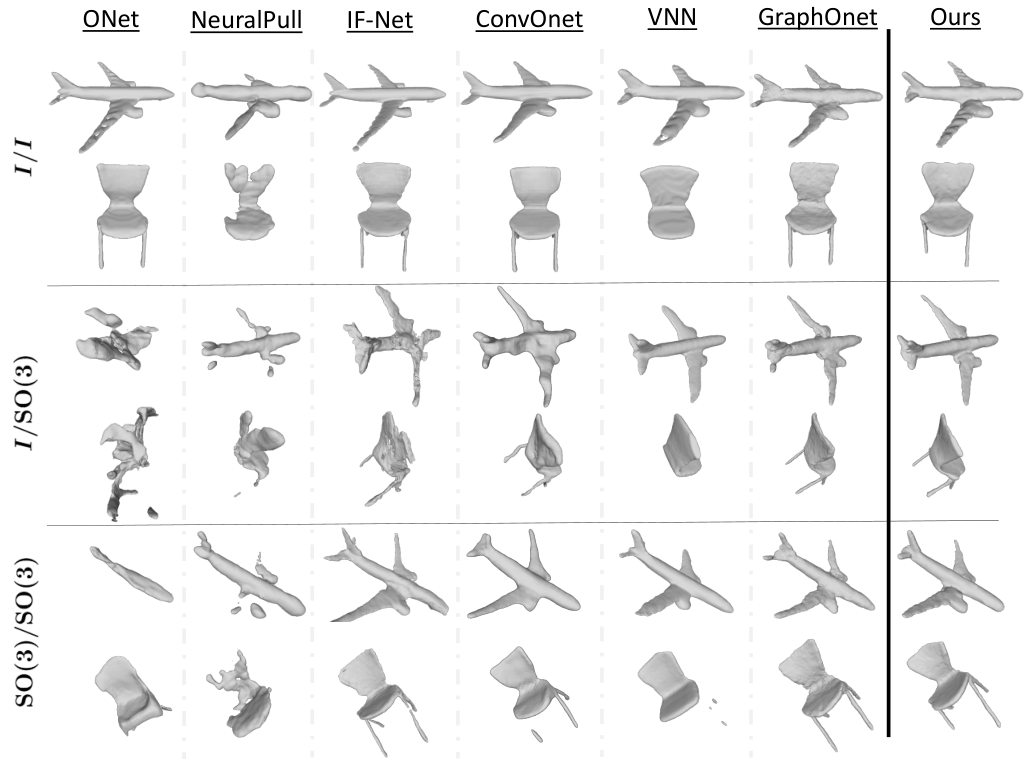
In Table 1, we present the F-Score (Tatarchenko et al. 2019), the Chamfer-L1 distance (Fan et al. 2017) and the Intersection over Union (IoU) of the reconstruction, for models trained on the aligned and $\mathrm{SO}(3)$-augmented datasets. We refer to section A.1 of the Appendix for a more detailed description of the evaluation metrics. Our method achieves consistent performance regardless of the rotation of the training or testing data points. Additionally, the best performance is achieved when we use up to type-2 representations in both the encoder and the decoder (E:0-2,D:0-2). When the testing data are transformed by random $\mathrm{SO}(3)$ rotations, our method consistently outperforms the compared methods, regardless of whether it is trained on rotated or aligned training data. In figure 4a, we show qualitative comparisons between the methods. Our model achieves consistently high quality reconstruction in all settings ($I/I$, $I/\mathrm{SO}(3)$, $\mathrm{SO}(3)/\mathrm{SO}(3)$). Finally, to study how the point cloud density and the added noise affects the reconstruction, we train in the original setting and evaluate on point clouds with different densities and levels of noise. As shown in figure 5b, our method outperforms previous methods on sparser point clouds, and scales better to denser point clouds.

In this section, we evaluate the ability of our model to reconstruct novel scenes with many different objects, while trained only on single objects. Due to SE(3)-equivariance, performance is consistent and independent of the pose and the position of the objects. Additionally, our method performs computations in local neighborhoods that usually contain points from a single object. These two factors allow us to reconstruct scenes that contain objects in arbitrary poses and positions, without the need to train on similar scenes, or to segment into separate objects and reconstruct each one. We construct a dataset of synthetic rooms with multiple objects from ShapeNet in arbitrary locations and poses, similarly to the dataset constructed in Peng et al. 2020, but with the addition of random SO(3) rotations on each object. We call this dataset the Seismic dataset.

In figure 5a we show a quantitative comparison between our method (TF-Onet [E:0-2,D:0-2]) and previous methods that lack either the local shape modeling or the equivariant property. Figure 4b shows a qualitative comparison between the reconstructions achieved by these methods, while Figure 6a shows more examples of the reconstruction achieved by our model for scenes from the seismic dataset. Methods that perform global shape modeling (OccNet, VNN) and are trained on single objects fail to generalize to scenes containing multiple objects. On the other hand, methods that perform local shape modeling but are not equivariant to SE(3) transforms (ConvOnet), can reconstruct objects in novel poses, but with reduced quality. Finally, the $\mathrm{SE}(3)$ equivariant GraphOnet, that uses per-point features with long range dependencies, cannot generalize well on novel scenes when it is only trained on single objects. Our method benefits from both equivariance and local shape modeling, and is able to generalize to novel scenes achieving quality similar to that on single object reconstruction. In Figure 6b, we also show examples of reconstructions of realistic scenes captured from the Matterport3D dataset (Chang et al. 2017). These scenes contain between 6000 to 13000 points. While our method has only been trained with aligned single objects from ShapeNet represented as point clouds of 300 points, it successfully reconstructs complicated realistic scenes containing multiple objects in arbitrary positions and poses, even from unseen classes.

References

- Alexa et al. (2003) M. Alexa, J. Behr, D. Cohen-Or, S. Fleishman, D. Levin, and C.T. Silva. Computing and rendering point set surfaces. IEEE Transactions on Visualization and Computer Graphics, 9(1):3–15, 2003. doi: 10.1109/TVCG.2003.1175093.
- Ba et al. (2016) Jimmy Lei Ba, Jamie Ryan Kiros, and Geoffrey E Hinton. Layer normalization. arXiv preprint arXiv:1607.06450, 2016.
- Bahdanau et al. (2015) Dzmitry Bahdanau, Kyunghyun Cho, and Yoshua Bengio. Neural machine translation by jointly learning to align and translate. In Yoshua Bengio and Yann LeCun (eds.), 3rd International Conference on Learning Representations, ICLR 2015, San Diego, CA, USA, May 7-9, 2015, Conference Track Proceedings, 2015. URL http://arxiv.org/abs/1409.0473.
- Baorui et al. (2021) Ma Baorui, Han Zhizhong, Liu Yu-Shen, and Zwicker Matthias. Neural-pull: Learning signed distance functions from point clouds by learning to pull space onto surfaces. In International Conference on Machine Learning (ICML), 2021.
- Berger et al. (2017) Matthew Berger, Andrea Tagliasacchi, Lee M Seversky, Pierre Alliez, Gael Guennebaud, Joshua A Levine, Andrei Sharf, and Claudio T Silva. A survey of surface reconstruction from point clouds. In Computer Graphics Forum, volume 36, pp. 301–329. Wiley Online Library, 2017.
- Boulch & Marlet (2022) Alexandre Boulch and Renaud Marlet. Poco: Point convolution for surface reconstruction. In Proceedings of the IEEE/CVF Conference on Computer Vision and Pattern Recognition (CVPR), pp. 6302–6314, June 2022.
- Brandstetter et al. (2022) Johannes Brandstetter, Rob Hesselink, Elise van der Pol, Erik J Bekkers, and Max Welling. Geometric and physical quantities improve e(3) equivariant message passing. In International Conference on Learning Representations, 2022. URL https://openreview.net/forum?id=_xwr8gOBeV1.
- Chabra et al. (2020) Rohan Chabra, Jan E. Lenssen, Eddy Ilg, Tanner Schmidt, Julian Straub, Steven Lovegrove, and Richard Newcombe. Deep local shapes: Learning local sdf priors for detailed 3d reconstruction. In ECCV 2020: 16th European Conference, pp. 608–625, 2020.
- Chang et al. (2017) Angel Chang, Angela Dai, Thomas Funkhouser, Maciej Halber, Matthias Niessner, Manolis Savva, Shuran Song, Andy Zeng, and Yinda Zhang. Matterport3d: Learning from rgb-d data in indoor environments. International Conference on 3D Vision (3DV), 2017.
- Chang et al. (2015) Angel X. Chang, Thomas Funkhouser, Leonidas Guibas, Pat Hanrahan, Qixing Huang, Zimo Li, Silvio Savarese, Manolis Savva, Shuran Song, Hao Su, Jianxiong Xiao, Li Yi, and Fisher Yu. ShapeNet: An Information-Rich 3D Model Repository. Technical Report arXiv:1512.03012 [cs.GR], Stanford University — Princeton University — Toyota Technological Institute at Chicago, 2015.
- Chen et al. (2021) Haiwei Chen, Shichen Liu, Weikai Chen, Hao Li, and Randall Hill. Equivariant point network for 3d point cloud analysis. In Proceedings of the IEEE/CVF Conference on Computer Vision and Pattern Recognition, pp. 14514–14523, 2021.
- Chen et al. (2022) Yunlu Chen, Basura Fernando, Hakan Bilen, Matthias Nießner, and Efstratios Gavves. 3d equivariant graph implicit functions, 2022. URL https://arxiv.org/abs/2203.17178.
- Chen & Zhang (2019a) Zhiqin Chen and Hao Zhang. Learning implicit fields for generative shape modeling. In Proceedings of the IEEE/CVF Conference on Computer Vision and Pattern Recognition (CVPR), June 2019a.
- Chen & Zhang (2019b) Zhiqin Chen and Hao Zhang. Learning implicit fields for generative shape modeling. In Proceedings of the IEEE/CVF Conference on Computer Vision and Pattern Recognition, pp. 5939–5948, 2019b.
- Chibane et al. (2020) Julian Chibane, Thiemo Alldieck, and Gerard Pons-Moll. Implicit functions in feature space for 3d shape reconstruction and completion. In IEEE Conference on Computer Vision and Pattern Recognition (CVPR). IEEE, jun 2020.
- Choy et al. (2016) Christopher B Choy, Danfei Xu, JunYoung Gwak, Kevin Chen, and Silvio Savarese. 3d-r2n2: A unified approach for single and multi-view 3d object reconstruction. In Proceedings of the European Conference on Computer Vision (ECCV), 2016.
- Cohen & Welling (2016) Taco Cohen and Max Welling. Group equivariant convolutional networks. In International conference on machine learning, pp. 2990–2999, 2016.
- Cohen et al. (2019) Taco Cohen, Maurice Weiler, Berkay Kicanaoglu, and Max Welling. Gauge equivariant convolutional networks and the icosahedral CNN. In Proceedings of the 36th International Conference on Machine Learning, volume 97, pp. 1321–1330, 2019.
- de Haan et al. (2021) Pim de Haan, Maurice Weiler, Taco Cohen, and Max Welling. Gauge equivariant mesh cnns: Anisotropic convolutions on geometric graphs. In 9th International Conference on Learning Representations, ICLR 2021, Virtual Event, Austria, May 3-7, 2021. OpenReview.net, 2021. URL https://openreview.net/forum?id=Jnspzp-oIZE.
- Deng et al. (2021) Congyue Deng, Or Litany, Yueqi Duan, Adrien Poulenard, Andrea Tagliasacchi, and Leonidas J. Guibas. Vector neurons: A general framework for so(3)-equivariant networks. In Proceedings of the IEEE/CVF International Conference on Computer Vision (ICCV), pp. 12200–12209, October 2021.
- Dosovitskiy et al. (2021) Alexey Dosovitskiy, Lucas Beyer, Alexander Kolesnikov, Dirk Weissenborn, Xiaohua Zhai, Thomas Unterthiner, Mostafa Dehghani, Matthias Minderer, Georg Heigold, Sylvain Gelly, Jakob Uszkoreit, and Neil Houlsby. An image is worth 16x16 words: Transformers for image recognition at scale. In International Conference on Learning Representations, 2021. URL https://openreview.net/forum?id=YicbFdNTTy.
- Erler et al. (2020) Philipp Erler, Paul Guerrero, Stefan Ohrhallinger, Niloy J. Mitra, and Michael Wimmer. Points2Surf: Learning implicit surfaces from point clouds. In Andrea Vedaldi, Horst Bischof, Thomas Brox, and Jan-Michael Frahm (eds.), Computer Vision – ECCV 2020, pp. 108–124, Cham, 2020. Springer International Publishing.
- Esteves et al. (2018) Carlos Esteves, Christine Allen-Blanchette, Ameesh Makadia, and Kostas Daniilidis. Learning so(3) equivariant representations with spherical cnns. In The European Conference on Computer Vision (ECCV), September 2018.
- Fan et al. (2017) Haoqiang Fan, Hao Su, and Leonidas J. Guibas. A point set generation network for 3d object reconstruction from a single image. In Proceedings of the IEEE Conference on Computer Vision and Pattern Recognition (CVPR), July 2017.
- Fuchs et al. (2020) Fabian B. Fuchs, Daniel E. Worrall, Volker Fischer, and Max Welling. Se(3)-transformers: 3d roto-translation equivariant attention networks. In Advances in Neural Information Processing Systems 34 (NeurIPS), 2020.
- Fukushima (1980) Kunihiko Fukushima. Neocognitron: A self-organizing neural network model for a mechanism of pattern recognition unaffected by shift in position. Biological cybernetics, 36(4):193–202, 1980.
- Fulton & Harris (2013) William Fulton and Joe Harris. Representation theory: a first course, volume 129. Springer Science & Business Media, 2013.
- Genova et al. (2020) Kyle Genova, Forrester Cole, Avneesh Sud, Aaron Sarna, and Thomas Funkhouser. Local deep implicit functions for 3d shape. In The IEEE Conference on Computer Vision and Pattern Recognition (CVPR), pp. 4856–4865, 06 2020. doi: 10.1109/CVPR42600.2020.00491.
- Gong et al. (2019) Shunwang Gong, Lei Chen, Michael Bronstein, and Stefanos Zafeiriou. Spiralnet++: A fast and highly efficient mesh convolution operator. In Proceedings of the IEEE/CVF International Conference on Computer Vision Workshops, pp. 0–0, 2019.
- Hall (2003) Brian C Hall. Lie groups, Lie algebras, and representations: an elementary introduction, volume 10. Springer, 2003.
- Jiang et al. (2020) Chiyu Max Jiang, Avneesh Sud, Ameesh Makadia, Jingwei Huang, Matthias Nießner, and Thomas Funkhouser. Local implicit grid representations for 3d scenes. In Proceedings IEEE Conf. on Computer Vision and Pattern Recognition (CVPR), 2020.
- Kazhdan & Hoppe (2013) Michael Kazhdan and Hugues Hoppe. Screened poisson surface reconstruction. ACM Trans. Graph., 32(3), jul 2013. ISSN 0730-0301. doi: 10.1145/2487228.2487237. URL https://doi.org/10.1145/2487228.2487237.
- Kendall (1989) David G Kendall. A survey of the statistical theory of shape. Statistical Science, 4(2):87–99, 1989.
- Kingma & Ba (2015) Diederik P. Kingma and Jimmy Ba. Adam: A method for stochastic optimization. In 3rd International Conference on Learning Representations, ICLR 2015, San Diego, CA, USA, May 7-9, 2015, Conference Track Proceedings, 2015.
- LeCun et al. (1989) Yann LeCun, Bernhard Boser, John S Denker, Donnie Henderson, Richard E Howard, Wayne Hubbard, and Lawrence D Jackel. Backpropagation applied to handwritten zip code recognition. Neural computation, 1(4):541–551, 1989.
- Lionar et al. (2021) Stefan Lionar, Daniil Emtsev, Dusan Svilarkovic, and Songyou Peng. Dynamic plane convolutional occupancy networks. In Winter Conference on Applications of Computer Vision (WACV), 2021.
- Lorensen & Cline (1987) William E Lorensen and Harvey E Cline. Marching cubes: A high resolution 3d surface construction algorithm. ACM siggraph computer graphics, 21(4):163–169, 1987.
- Maron et al. (2019) Haggai Maron, Heli Ben-Hamu, Nadav Shamir, and Yaron Lipman. Invariant and equivariant graph networks. In 7th International Conference on Learning Representations, ICLR 2019, New Orleans, LA, USA, May 6-9, 2019, 2019.
- Mescheder et al. (2019) Lars Mescheder, Michael Oechsle, Michael Niemeyer, Sebastian Nowozin, and Andreas Geiger. Occupancy networks: Learning 3d reconstruction in function space. In Proceedings IEEE Conf. on Computer Vision and Pattern Recognition (CVPR), 2019.
- Niemeyer & Geiger (2021) Michael Niemeyer and Andreas Geiger. Giraffe: Representing scenes as compositional generative neural feature fields. In Proceedings of the IEEE/CVF Conference on Computer Vision and Pattern Recognition, pp. 11453–11464, 2021.
- Niemeyer et al. (2020) Michael Niemeyer, Lars Mescheder, Michael Oechsle, and Andreas Geiger. Differentiable volumetric rendering: Learning implicit 3d representations without 3d supervision. In Proceedings of the IEEE/CVF Conference on Computer Vision and Pattern Recognition, pp. 3504–3515, 2020.
- Pan et al. (2021) Xuran Pan, Zhuofan Xia, Shiji Song, Li Erran Li, and Gao Huang. 3d object detection with pointformer. In Proceedings of the IEEE/CVF Conference on Computer Vision and Pattern Recognition (CVPR), pp. 7463–7472, June 2021.
- Park et al. (2019) Jeong Joon Park, Peter Florence, Julian Straub, Richard Newcombe, and Steven Lovegrove. Deepsdf: Learning continuous signed distance functions for shape representation. In The IEEE Conference on Computer Vision and Pattern Recognition (CVPR), June 2019.
- Peng et al. (2020) Songyou Peng, Michael Niemeyer, Lars Mescheder, Marc Pollefeys, and Andreas Geiger. Convolutional occupancy networks. In European Conference on Computer Vision, pp. 523–540. Springer, 2020.
- Poulenard & Guibas (2021) Adrien Poulenard and Leonidas J. Guibas. A functional approach to rotation equivariant non-linearities for tensor field networks. In Proceedings of the IEEE/CVF Conference on Computer Vision and Pattern Recognition (CVPR), pp. 13174–13183, June 2021.
- Qi et al. (2016) Charles R. Qi, Hao Su, Kaichun Mo, and Leonidas J. Guibas. Pointnet: Deep learning on point sets for 3d classification and segmentation, 2016. URL http://arxiv.org/abs/1612.00593. cite arxiv:1612.00593.
- Riegler et al. (2017) Gernot Riegler, Ali Osman Ulusoy, and Andreas Geiger. Octnet: Learning deep 3d representations at high resolutions. In Proceedings of the IEEE conference on computer vision and pattern recognition, pp. 3577–3586, 2017.
- Romero & Cordonnier (2021) David W. Romero and Jean-Baptiste Cordonnier. Group equivariant stand-alone self-attention for vision. In International Conference on Learning Representations, 2021. URL https://openreview.net/forum?id=JkfYjnOEo6M.
- Sitzmann et al. (2019) Vincent Sitzmann, Michael Zollhöfer, and Gordon Wetzstein. Scene representation networks: Continuous 3d-structure-aware neural scene representations. Advances in Neural Information Processing Systems, 32, 2019.
- Tang et al. (2021) Jiapeng Tang, Jiabao Lei, Dan Xu, Feiying Ma, Kui Jia, and Lei Zhang. Sa-convonet: Sign-agnostic optimization of convolutional occupancy networks. In Proceedings of the IEEE/CVF International Conference on Computer Vision, 2021.
- Tatarchenko et al. (2019) Maxim Tatarchenko, Stephan R. Richter, Rene Ranftl, Zhuwen Li, Vladlen Koltun, and Thomas Brox. What do single-view 3d reconstruction networks learn? In Proceedings of the IEEE/CVF Conference on Computer Vision and Pattern Recognition (CVPR), June 2019.
- Thomas et al. (2018) Nathaniel Thomas, Tess Smidt, Steven Kearnes, Lusann Yang, Li Li, Kai Kohlhoff, and Patrick Riley. Tensor field networks: Rotation-and translation-equivariant neural networks for 3d point clouds. arXiv preprint arXiv:1802.08219, 2018.
- Tretschk et al. (2020) Edgar Tretschk, Ayush Tewari, Vladislav Golyanik, Michael Zollhöfer, Carsten Stoll, and Christian Theobalt. PatchNets: Patch-Based Generalizable Deep Implicit 3D Shape Representations. European Conference on Computer Vision (ECCV), 2020.
- Vaswani et al. (2017) Ashish Vaswani, Noam Shazeer, Niki Parmar, Jakob Uszkoreit, Llion Jones, Aidan N Gomez, Ł ukasz Kaiser, and Illia Polosukhin. Attention is all you need. In I. Guyon, U. V. Luxburg, S. Bengio, H. Wallach, R. Fergus, S. Vishwanathan, and R. Garnett (eds.), Advances in Neural Information Processing Systems, volume 30. Curran Associates, Inc., 2017.
- Wang & Zhang (2022) He Wang and Juyong Zhang. A survey of deep learning-based mesh processing. Communications in Mathematics and Statistics, pp. 1–32, 2022.
- Weiler et al. (2018a) Maurice Weiler, Mario Geiger, Max Welling, Wouter Boomsma, and Taco Cohen. 3d steerable cnns: Learning rotationally equivariant features in volumetric data. In NeurIPS, 2018a.
- Weiler et al. (2018b) Maurice Weiler, Fred A. Hamprecht, and Martin Storath. Learning steerable filters for rotation equivariant cnns. In 2018 IEEE Conference on Computer Vision and Pattern Recognition, CVPR 2018, Salt Lake City, UT, USA, June 18-22, 2018, pp. 849–858. IEEE Computer Society, 2018b.
- Weiler et al. (2021) Maurice Weiler, Patrick Forré, Erik Verlinde, and Max Welling. Coordinate independent convolutional networks - isometry and gauge equivariant convolutions on riemannian manifolds. CoRR, abs/2106.06020, 2021. URL https://arxiv.org/abs/2106.06020.
- Williams et al. (2022) Francis Williams, Zan Gojcic, Sameh Khamis, Denis Zorin, Joan Bruna, Sanja Fidler, and Or Litany. Neural fields as learnable kernels for 3d reconstruction. In Proceedings of the IEEE/CVF Conference on Computer Vision and Pattern Recognition (CVPR), pp. 18500–18510, June 2022.
- Wu et al. (2021) Haiping Wu, Bin Xiao, Noel Codella, Mengchen Liu, Xiyang Dai, Lu Yuan, and Lei Zhang. Cvt: Introducing convolutions to vision transformers. In Proceedings of the IEEE/CVF International Conference on Computer Vision (ICCV), pp. 22–31, October 2021.
- Wu et al. (2019) Wenxuan Wu, Zhongang Qi, and Li Fuxin. Pointconv: Deep convolutional networks on 3d point clouds. In Proceedings of the IEEE/CVF Conference on Computer Vision and Pattern Recognition (CVPR), June 2019.
- Yu et al. (2021) Xumin Yu, Yongming Rao, Ziyi Wang, Zuyan Liu, Jiwen Lu, and Jie Zhou. Pointr: Diverse point cloud completion with geometry-aware transformers. In ICCV, 2021.
- Zhu et al. (2021) Minghan Zhu, Maani Ghaffari, and Huei Peng. Correspondence-free point cloud registration with SO(3)-equivariant implicit shape representations. In 5th Annual Conference on Robot Learning, 2021. URL https://openreview.net/forum?id=KOq9qDgn-Ta.
Appendix A Appendix
A.1 Evaluation Metrics
In table 1, we present the F-Score, Chamfer-L1 distance and Intersection over Union (IoU) of the reconstruction achieved by various models. For the F-Score and Chamfer-L1 distance, we compute the reconstructed mesh using the Marching Cubes algorithm (Lorensen & Cline 1987). Then, we uniformly sample 100,000 points from the reconstructed mesh, and compare them with the “ground truth” points sampled similarly from the “ground truth” mesh. The standard deviation of the results for both metrics due to the randomness introduced by the sampling of the 100,000 points is smaller than . As defined in Tatarchenko et al. 2019, the F-Score here is the harmonic mean of the precision and the recall of the reconstruction Precision is the percentage of reconstructed points that lie within a certain distance of the ground truth points, and recall is the percentage of ground truth points that lie within a distance of the reconstructed points. We compute the F-Score with equal to of the side length of the reconstructed volume and with equal to of the side length of the reconstructed volume. For the IoU metric, we uniformly sample 100,000 points from the whole space, and compare the predicted occupancy to the ground truth occupancy. The IoU is then computed by taking the ratio of points that are occupied according to both the predicted and the ground truth occupancy to the points that are occupied according to either the predicted or the ground truth occupancy.
A.2 Model Architecture, Training and Testing Details
For the self-attention feature extractor network , we use ten multi-headed SE(3) attention layers, and for the cross-attention occupancy network we use another two. All multi-headed SE(3) attention layers use eight heads. For each point of the point cloud, we define the neighborhood as its nearest neighbors, where is chosen to be of the size of the point cloud (e.g., for 300 points, =15). Each feature map in the layers of uses irreducibles up to type-2.
We train our model on the ShapeNet (Chang et al. 2015) subset constructed in Choy et al. 2016. We use the Adam (Kingma & Ba 2015) optimizer with learning rate that starts at and linearly decreases to reach the value of . We train for 200,000 iterations using a batch size of 64. During training, we take as input a point cloud of 300 points and as ground truth the occupancy value of 2048 points that are sampled uniformly inside a box that bounds the object. As a training loss, we use the binary cross-entropy loss between the predicted and the ground truth occupancy of the 2048 randomly sampled points.
During inference, recalling that the output of our model for one query point is in the range of , we classify a query point as occupied if the value of the learned occupancy function is above . After we query the occupancy of points throughout the space, we reconstruct the object’s mesh using the Marching Cubes algorithm (Lorensen & Cline 1987).
A.3 Extracting Different Types of Representations as Features
An important quality of our method is its ability to use different types of representations as its intermediate features. These different types determine the way that the features transform as the input rotates. These transformation laws affect the shape properties that each type of features can encode. For example type-0 features can encode properties of the shape that are invariant to the rotation of the shape, type-1 features can encode properties that must rotate as 3d vectors (e.g. the normal vectors at the surface) and type-2 features can encode properties that rotate as symmetric matrices (e.g. the inertial matrix of the shape).
A type feature consists of a dimensional vector that rotates according to the corresponding Wigner-D matrix . In figure 7 we visualize the different types of features extracted by our encoder for different cases of inputs. The difference between the type of features can be clearly observed in the case of the symmetric sphere where features of higher type correspond to higher frequencies on the sphere.
A.4 Reconstructions of Scanned Scenes
We further investigate the generalization of our method to novel scenes by reconstructing real objects of different domains and levels of clutter (Fig. 8). The input is a sparse, unoriented point cloud scanned from scenes consisting of an arbitrary number of randomly placed objects. The model is agnostic to the number of objects in the scene and is trained only on synthetic single objects. The model outputs high-quality reconstructions even in difficult settings with objects very close to each other. We observe small artifacts in very cluttered scenes, localized in regions of incidence between objects (e.g. mugs in line 4 of Fig. 8).
A.5 Robustness to clutter
We evaluate the model on the Seismic dataset (Sec. 4.2) which contains scenes with varying levels of clutter. In Fig. 9 we measure the Intersection over Union (IoU) of the reconstruction versus the minimum distance between any two objects in the scene (normalized with respect to the room size). The minimum distances range from around to of the room. The performance of the model is relatively stable across all settings with a maximum performance decrease of in IoU.
A.6 Limitations and Future Work
A possible limitation of this work is the inherent memory overhead of the attention modules used in the network. In our setting, this overhead is lowered due to the locality of the attention operation but it can be further minimized with additional optimization of the attention modules. The optimization of the attention modules is an active research direction that can also benefit our method. An additional possible direction for future work is to extend our method to the problem of scene completion from partial observations. In this task, the model is required to hallucinate and reconstruct unobserved areas of a scene and thus requires a combination of local and global information about the scene configuration. While a significant methodological extension is required for our method to tackle such a task we believe that the core principles of equivariance via higher-order representations and local shape modeling can provide useful tools.
A.7 Weight Parametrization
Here, we present the parametrization of the weights of the queries, keys, and values that appear as the solutions of Equation 3.3 (and written analytically in Equation 3.3). We focus on the specific case where both the input and output feature maps are -fields consisting of up to type-2 irreducibles. Then, each feature in the feature maps can be decomposed into
For clarity, we start with multiplicities 1 i.e., (and omit the index of the layer). Then we extend to the general case.
The matrix appearing in the query tokens has the form:
Similarly, we present the form of the function of matrices , that appear in the key tokens as . To simplify the notation we use instead of and . To write in matrix form we first need to define:
The functions are parametrized by MLPs. are fixed matrices defined in Section 3.3. Given the definition above we can write as:
The form of the matrices appearing in the value tokens as is similar to above.
In the general case, if the input representation contains copies of type-k irreducibles we need to stack the corresponding blocks of , times in the column dimension. Similarly, if the output representation contains copies of type- irreducibles we need to stack the corresponding blocks times in the row dimension. Specifically,
- •
for and :
A.8 Preliminaries
We recall some basic notions from group and representation theory, see e.g., Fulton & Harris 2013. A group is a set together with a binary operator “” that satisfies the following axioms:
Associativity: for all
Identity: there exists an element such that
Inverse: for all , there exists such that .
Given , we say that each group element acts on the space via an action if satisfy the following two properties:
If is the identity element of then for all ;
for all .
If for any there exists such that , then we call a homogeneous space for the group .
When is a vector space, we can define the group action using a linear group representation , where is a map from group to the general linear group . This means that using the linear operator on , we can define the group action on the vector space as for all , . Then is a linear group representation if is a group homomorphism, i.e., for all , and is the identity operator over . To simplify the notation, when the vector space that the group acts on is easily inferred from the context, we will use to denote the representation .
Given a set of actions for , and a set of actions for , we say that a map is -equivariant if for every :
If is linear and equivariant (with respect to ), then it is called an intertwiner (with respect to ).
If there exists a subspace such that for all and , we have that , then is a -invariant subspace of , and is a subrepresentation of . All representations have at least two subrepresentations: and . If a representation has no other subrepresentations, then it is called irreducible. Otherwise it is called reducible. A fundamental result is the following (Fulton & Harris 2013).
A.8.1 Schur’s Lemma
Let , be irreducible representations of acting on and , respectively.
If and are not isomorphic, then there are no nontrivial intertwiners between them.
If are finite-dimensional vector spaces over , and if , then all intertwiners are scalar multiples of the identity.
Now we list a number of fundamental examples, see e.g., Fulton & Harris 2013; Hall 2003.
A.8.2 The translation group :
equipped with the addition operator “” is a group that is isomorphic to the group of translations in the 3D space.
A.8.3 The special orthogonal group SO(3):
is the group of orthogonal matrices with determinant equipped with multiplication; and is isomorphic to the group of all 3D rotations about the origin. is a compact group and as a result of the Peter-Weyl theorem, its linear representations can be decomposed into a direct sum of finite-dimensional, unitary, irreducible representations. Specifically a linear representation of decomposes as:
where is a change of basis matrix and are matrices known as the Wigner D-matrices. The Wigner D-matrices are the irreducible representations of . In the context of the features of a neural net, the representations (viewed as vectors) that transform according to are called type- vectors.
A.8.4 The special Euclidean group :
is the group of proper rigid transformations of 3D space, and is isomorphic to the semidirect product . An element of can be represented as where is an element of the group of translations and is an element of the group of 3D rotations. For two elements , the group law is defined as:
Since every point in can be transformed into any other point with a proper rigid transformation, we have that is a homogeneous space for .
In addition to the action of on vectors in , we can also define the action of on functions , for any given integer . This action is called the induced representation of . It acts on as follows:
where , and is a representation of . Especially in the context of neural nets where functions are viewed as feature fields, a function that transforms according to is called a -field, and if corresponds to the -th irreducible representation of , it is also called a field of type-.
A.9 Architecture Details
A feature-augmented point cloud where and for some can be associated with a 3d field of finite support by writing . This association will be useful to define the group action on the feature-augmented point cloud and will unify the inputs and outputs of in the sense that both of them process fields in and output fields in . We will interchangeably use and for the point cloud in the next sections. We will call the point cloud function when the distinction is not clear.
The main module in our architecture is an -equivariant attention block. Each block consists of a multi-head -equivariant attention module followed by a skip connection and an equivariant layer normalization step.
A.9.1 Multi-head -equivariant Attention Module:
This module consists of multiple heads that implement either self-attention (input features for keys, values and queries are the same) or cross-attention (input features for keys and values are the same and different from the inputs for the queries). We will first describe the self-attention variant of the module and then describe the changes that are required for the cross-attention version.
The self-attention -equivariant module takes as input a function (describing the point cloud as discussed above) defined by . Each one of the vectors can be decomposed into irreducible representations of appearing with different multiplicities. This means that a single vector can be decomposed as , where corresponds to the -th multiplicity of the irreducible component of type-. Since we perform self-attention, the keys, values and queries are computed using the same input function . Specifically, for pairs of key and query points , we compute the keys , the queries , and the values . To ensure equivariance, , , must satisfy the conditions described in Section 3.3.
Suppose that for the computed key and query features, the -th irreducible appears with multiplicity , and for the computed value features the -th irreducible appears with multiplicity . For each irreducible, we split its multiplicities across the different heads of the attention block. Assuming that we have heads in total, each head receives keys and queries containing irreducibles with multiplicities and receives values containing irreducibles appearing with multiplicities . After this split, the output of the self-attention for each head can be computed as:
where
Similar to the keys, values and queries, the output can have irreducibles and multiplicities that differ from the input and decompose as:
where is the -th multiplicity of the -th irreducible.
After the application of the self-attention layer, we concatenate the output of all the heads to create . Then we pass the concatenated output through a linear -equivariant layer to take . Since this linear layer also needs to be equivariant, it must follow the same constraints as the query matrix . By Schur’s lemma, it follows that can only mix feature vectors that correspond to the same irreducibles.
For implementing cross-attention, we use the same process as with self-attention, with the only difference that the inputs for the queries are different from the inputs for the keys and the values. As a result, the output of the cross-attention for a single head is computed as:
A.9.2 Skip connection:
The skip connection concatenates the output features of the multi-headed -equivariant module with the features of the input query. To respect the type of each feature, this concatenation must happen between features corresponding to the same irreducible.
Suppose that is the output of the multi-head attention, decomposing into irreducibles and their multiplicities as . Similarly suppose that is the input query, decomposing into irreducibles and their multiplicities as . The application of the skip connection gives an output
To keep the output at the same types and multiplicities as specified by the user (i.e., to be a -field) we only concatenate multiplicities from the input that exist in the output. Also, after the skip connection we apply an equivariant linear layer between irreducibles of the same type to project the features to the correct dimensions.
A.9.3 Equivariant Layer Norm:
Suppose that denotes the -th type- irreducible of the input vector . As proposed in Fuchs et al. 2020, for each vector , we apply layer normalization and a nonlinearity on the norm of , leaving its direction unchanged. Thus, the equivariant normalization layer can be written as:
where corresponds to layer normalization, proposed in Ba et al. 2016.
We use the -equivariant attention block to construct both the network that assigns to each point in the point cloud a learned feature, and the network , that outputs the occupancy value of a query point in space. The network consists of ten -equivariant self-attention blocks, and consists of two -equivariant cross-attention blocks. Figure 2 shows a diagram of this architecture.
In both networks, we use blocks with eight heads and intermediate representations that contain features up to type-2. Additionally, for each type we set the multiplicity of the corresponding irreducible to 32. Finally, for the computation of the local neighborhood around each point , we use the nearest neighbors, where is chosen to be of the size of the point cloud (e.g., for 300 points, =15).
Although it is possible for to output a single scalar that corresponds to the occupancy value at a queried point, we observe in the experiments an increase in performance when outputs 32 scalar values that we then pass through a simple MLP to get the final occupancy value.
A.10 Proofs on Equivariance from Sec.3.3
1. Input-output equivariance (Eq. 3): We will formalize the equivariance constraints in the language of group theory. We have a map that takes as input a point cloud and outputs an occupancy field . First we need to define the actions of SE(3) on the input point cloud and the occupancy map which we denote by , respectively. Those have the following form for :