Accurate benchmark results of Blasius boundary layer problem using a leaping Taylor’s series that converges for all real values.
Abstract
Blasius boundary layer solution is a Maclaurin series expansion of the function , which has convergence problems when evaluating for higher values of due to a singularity present at . In this paper we are introducing an accurate solution to using Taylor’s series expansions with progressively shifted centers of expansion(Leaping centers). Each series is solved as an IVP with the three initial values computed from solution of the previous series, so the gap between the centers of two consecutive expansions is selected from within the convergence disc of the first series. The last series is formed such that it is convergent for a reasonable high value needed for implementing the boundary condition at infinity. The present methodology uses Newton-Raphson method to compute the value of the unknown initial condition viz. in an iterative manner. Benchmark accurate results of different parameters of flat plate boundary layer with no slip and slip boundary conditions have been reported in this paper.
Keywords:
Blasius function , Leaping Taylor’s series , Slip flow , Newton-Raphson method1 Introduction
Blasius series solution [1, 2] is well known as the accurate solution for flat plate boundary layer flow. It is not only a remarkable achievement in the history of fluid dynamics but also a groundbreaking mathematical exercise in which the non-linear differential equation with the known conditions , called the Blasius boundary layer equation is solved. It is not an initial value problem because is not known and this poses certain difficulties in determining its solution. The function represents the value of stream function and is popularly known as the Blasius function. Blasius determined the solution in the form of a power series expansion [3] as,
| (1) |
where . The above series with center of expansion at is found to have convergence problems at certain values of and due to this the value of is often found with a lesser accuracy. Understanding the mathematical nature of Blasius function including convergence properties, obtaining better accurate solutions and extension to cases of slip boundary conditions etc, have prompted the researchers to further investigate and solve the problem analytically [4, 5] and numerically [6, 7].
Along with analytical methods, there have been efforts to use finite-order accurate numerical techniques such as Runge-Kutta method and shooting method for getting the unkknown initial condition etc., due to the ease of computation. The shooting method [8] is used extensively, such that it has literally become a part of classroom exercises. The shooting method is a technique for solving a BVP by reducing it into an IVP. The method consists of solving IVP with different initial conditions until the boundary condition of the BVP is satisfied. Another technique used to deduce the initial condition is called Töpfer transformation () [9, 10]. Töpfer transformation leaves the initial conditions unchanged along with the introduction of an additional initial condition, leading to the computation of the Blasius function and its derivatives through an inverse transformation. A number of previous investigations have reported the use of the Runge-Kutta scheme along with the shooting method [6, 11] to determine the unknown initial condition of the problem. One of the historical literature on numerical method adopted for solving the Blasius equation is by Howarth [12] in which the value of , accurate upto five decimal places is reported. A recent study by Majid et al.[13] uses a predictor-corrector two-point block method to solve the Blasius equation numerically. The idea revolves around the development of a technique to bypass the step of reducing the BVP to an IVP, thus it makes use of a multiple shooting method that converges faster .
Previous studies on solutions to Blasius function have also been attempted using analytical or semi-analytical methods with an aim to get the solution with higher accuracy and with out convergence difficulties. Adomian Decomposition Method (ADM) is a semi-analytical method that uses ”Adomain Polynomials” to represent the non-linear portion of the function. Abbaoui et al. [14] have given a proof for the convergence of the series solutions obtained from Adomaian Decomposition Method. Wang [15] has shown the application of ADM to obtain an approximate analytical solution to Blasius function. Hashim [16] presents a modified technique that uses a combined ADM and Pade approach to report the improvement in the accuracy of the solution. Boyd [17] reported that series solution alone is not enough and combining it with the Pade approximation is an effective approach. Pade approximation provides very close estimate of the function by writing it in the form of a rational function of a given order. It is reported that Pade Approximation to Blasius equation with provides convergence to the solution with a relative error of about in predicting the accurate value of . For , the convergence is found to be slow and there is a need for higher values of Pade order (N) for getting a better solution. A recent study by Andrianov et al. [18] introduced the Pade approximation for solving the boundary layer problem and for the problem of rotating fluid of Ekman layer type.
Differential Transformation Method (DTM) is a systematic framework that gives transformations which becomes the coefficients of terms of the series expansion of a function or functions presented in the form of linear, non-linear and simultaneous ordinary differential equations [19, 20, 21, 22]. It may be noted that Blasius has derived his series accurately in the same manner but without resorting to DTM framework. Yu et. al. [19], used DTM by converting the Blasius problem into a set of three IVPs. A sub-domain approach is found to overcome the convergence problems of the series solution and values accurate up to decimal places are reported. Arikoglu and Ibrahim [23] have presented an inner-outer matching solution for the Blasius problem in which is evaluated by equating two series expansions with one series expanded about and the other one about a higher value of of about . The matching of the solutions is done at a value of in between and to determine and the reported value is found to have a difference starting from the fourth decimal place onward. Lal and Neeraj [22] have used DTM along with the scaled transformation for converting the boundary value of Blasius function to initial value and reported results accurate up to 21 decimal points with a larger radius of convergence.
In the present work, we report a method in which a set of leaping series solutions that converge for all positive real values of are developed, with out resorting to approximations. Application of Newton-Raphson method enables determination of any unknown initial value in the problem from a suitable boundary condition, and still obtain Taylor’s series solution. Currently used methods such as Töpfer transformation, truncated boundary approximation, iterative transformation method [9, 10] are expected to pose difficulties in deriving the initial conditions from boundary conditions for the class problems governed by simultaneous differential equations and equations with more number of unknown initial values. We report benchmark solutions to boundary layers with no-slip and slip flow over the wall surface, nature of convergence of series expansions, unknown initial values and parameters of asymptotic variation with a greater accuracy in this paper.
2 Differential Transform
The Taylor series expansion of a function about is,
| (2) |
Where, , is called the differential transform of and is the derivative of with respect to . We denote differential transform operation of as and the result of the transform as . Let and are the differential transforms of the functions and . Some useful theorems of differential transforms with and [24, 25, 26] that becomes handy in finding the solutions of IVPs are given here.
Theorem 1
If , then
Theorem 2
If , then
Theorem 3
If , then
Theorem 4
If , then
Theorem 5
If , then
Making use of these theorems the terms in the Blasius equation namely and can be differential transformed as
| (3) |
| (4) |
By knowing , , the value of taken based on generated values of , the differential transform for any value of is found using
| (5) |
For , we have , and , where .
3 Solution Methodology
3.1 Series expansion about leaping centers
It is well known that Taylor’s series given in equation (1) with center of expansion at does not converge for [3]. But in computations on computers, convergence up to is rarely possible due to accuracy problems and restricted summation over a finite number of terms. This leads to approximating the boundary condition as , which results in lesser accurate results. In the present work, we propose an approach of combining more number of series expansions of the Blasius function by leaping the center of expansion to different values of to circumvent the convergence problems associated with approximation of . We have approximated the infinity by a larger value of and applied the boundary condition as , where . Such an approximation is found to provide a more accurate solution to the Blasius function.

The idea used in the present approach is to generate a few Taylor series expansions for with centers of expansion denoted as , as illustrated in Figure(1). The corresponding Taylor’s series expansions are denoted as for the functions , respectively. It may be noted that , because all the series expansions are for the same function, but the difference is only in their convergence properties. We use Differential Transform method described in the above section to compute the coefficients of the Taylor’s series. The coefficients of the series expansions are denoted by for all the values of . The initial condition for are , for no-slip flow and , a prescribed values of slip flow. We keep , a variable which is varied during the computation of Taylor’s series coefficients.
The initial conditions for computing any series with center of expansion at , namely, are taken from the already obtained series as,
| (6) |
Note that should converge at . So fixing an for expanding a series depends on the convergence of at . By following this procedure, it is possible to develop any number of series expansions. But an accurate solution can be obtained from as low as three series expansions, which is going to be demonstrated in the section on results.
3.2 Newton-Raphson Iteration
We first develop the selected number of function expansions, , and , by using a guessed value for , say . We then develop one more set of expansion namely, , corresponding to a slightly different value for , denoted as , where is a very small value. A typical value for used in the present computations is . It is found that is a strong boundary condition for the problem compared to . So we solve the equation for finding the converged solution for . The converged solution of is denoted as . In the present computations the condition at infinity is changed to the one corresponding to a very high value of denoted as . So we use as the equation solved for the determination of . We have used a value for in the range , where is a finite value of at which becomes almost equal to 1. The approximate gradient for Newton-Raphson method is computed as,
| (7) |
is now updated as,
| (8) |
Now, is assigned as the new value of and the computation of series is continued till becomes equal to 1 and this stage the value of is treated as the converged value for . The number of Newton-Raphson iterations applied to reach the solution for is kept as .
4 Results and discussion
The methodology for the solution has been implemented in FORTRAN with variable type for computations set using "IMPLICIT REAL*16(A-H,O-Z)" so as to get accuracy up to 32 decimal places in the floating point operations. All the results we report here are obtained from summing terms of the Taylor’s series. We find no difference in the converged value of with further increase in the number of terms of Taylor’s series summed.
4.1 Flow with no-slip


| n | ||
|---|---|---|
| 1 | 5 | 0.3361523439045316853836761393072 |
| 2 | 10 | 0.3320573372037024527094809622944 |
| 3 | 15 | 0.33205733621519629893842022877817 |
| 4 | 20 | 0.33205733621519629893718006201058 |
| 5 | 25 | 0.33205733621519629893718006201058 |
| 6 | 30 | 0.33205733621519629893718006201058 |
Table 1 shows the effect of number of expansions on the converged solution of by leaping the center of expansion by . Which means for every , the center of expansion , with . The number of iterations of Newton-Raphson step is kept as and this is found to guarantee the convergence of , up to decimal places. It can be seen that the converged solution is independent of for . This implies that the boundary condition at infinity can be well approximated at . More precisely, we find that the value of does not change from onward. We have also examined the effect of change of separation between the center of expansions and the observations are tabulated in Table 2. It can be seen that the result is independent on the step size of leaping of the center of expansion and is only dependent on the point , where the boundary condition is applied.
The value of resulted from the present computation has 32 decimal points accuracy, the accuracy is better than that of 0.33205733621519630 as given by Boyd in [3] and 0.332057336215196299183 as given by Lal and Neeraj in [22].
| n | |||
|---|---|---|---|
| 2 | 10 | 20 | 0.33205733621519629893718006201058 |
| 3 | 7 | 21 | 0.33205733621519629893718006201058 |
| 4 | 5 | 20 | 0.33205733621519629893718006201058 |
| 5 | 4 | 20 | 0.33205733621519629893718006201058 |
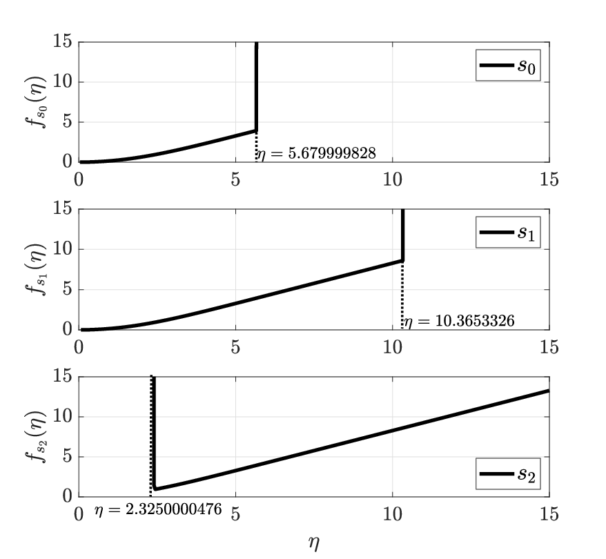
The convergence properties of the series expansions for , and having centers of expansion at , and are depicted in Figure 2 for . It can be seen that the series converges smoothly up to , which is close to the value corresponding to the singularity at as reported by Boyd in [3]. The series is found to be converging for and diverges for . The series is converging for and diverges for . The radius of convergence increases with the increase in distance of center of expansion from . These observations on the convergence implies that a single series can not represent the expansion of Blasius function for a larger domain.
By considering the convergence properties, we propose to use a combination of leaping series expansions to represent Blasius function as demonstrated in Figure (3). It consists of expansions, namely to with centers of expansion at , , for determining the convergence properties upto . The series expansion is used to determine the value of the function in the converging interval, . Figure (3) demonstrates the expansion of the function in the interval . In the same manner, by combining more number of series expansions, it is possible to expand the function for any positive real value. As per the results obtained in the present study found to be an optimum point where the boundary condition can be applied. From onward the asymptotic variation of the function is as . The parameter in the asymptotic variation has more decimal points accuracy than the one reported by Boyd in [3]. Tables 3 and 4 gives the benchmark results of the present accurate solutions of , , and for . It can be seen that the data satisfy the equation almost accurately.
| 0. | 0.00000000000000000000000000000000 | 0.00000000000000000000000000000000 |
| 1. | 0.16557172578927971994607139866464 | 0.32978003124966696806286485058647 |
| 2. | 0.65002436993528859325840008060347 | 0.62976573650238585970789214001077 |
| 3. | 1.39680823087034546785665318114741 | 0.84604444365799349725098240374192 |
| 4. | 2.30574641846207117902246203651341 | 0.95551822981069424686181417757482 |
| 5. | 3.28327366515631417796776890035073 | 0.99154190016439334277083771840218 |
| 6. | 4.27962092251384908051614632858349 | 0.99897287243586052111975290945127 |
| 7. | 5.27923881102910880195475622555865 | 0.99992160414795010955867185310631 |
| 8. | 6.27921343134607434184668676342406 | 0.99999627453530080913338909825509 |
| 9. | 7.27921237064524251498448401453620 | 0.99999989045379928945150717872348 |
| 10. | 8.27921234293432582800203409779852 | 0.99999999801539054606962551624450 |
| 11. | 9.27921234248405790426225183944242 | 0.99999999997791640300822743404095 |
| 12. | 10.27921234247952546306776851892884 | 0.99999999999984941269916627913591 |
| 13. | 11.27921234247949728852564004547502 | 0.99999999999999937182753490370178 |
| 14. | 12.27921234247949718064881057910890 | 0.99999999999999999839911378268159 |
| 15. | 13.27921234247949718039492878137463 | 0.99999999999999999999751013528420 |
| 0. | 0.33205733621519629893718006201058 | 0.00000000000000000000000000000000 |
| 1. | 0.32300711668694284746919034374890 | -0.02674042287603818941557199292502 |
| 2. | 0.26675154569727845645745365043572 | -0.08669750271056888580038083842490 |
| 3. | 0.16136031954087853155687842360081 | -0.11269471123528408855663373868942 |
| 4. | 0.06423412109169066819653982932531 | -0.07405379732511237191225366739570 |
| 5. | 0.01590679868531816315507141064886 | -0.02611318661022410269690678475316 |
| 6. | 0.00240203984375727885991930092577 | -0.00513990998602777383188838650274 |
| 7. | 0.00022016895527113462513633196741 | -0.00058116224682555289777061646404 |
| 8. | 0.00001224092624325319054622340463 | -0.00003843169423937603885233795627 |
| 9. | 0.00000041278790156878232013889098 | -0.00000150238539977608548717786204 |
| 10. | 0.00000000844291586701753292682574 | -0.00000003495034662828381184818483 |
| 11. | 0.00000000010473955482006946773795 | -0.00000000048595028491633710186547 |
| 12. | 0.00000000000078810075727866872385 | -0.00000000000405052751566817613004 |
| 13. | 0.00000000000000359671084986261923 | -0.00000000000002028403270505018845 |
| 14. | 0.00000000000000000995593526876784 | -0.00000000000000006112552161659052 |
| 15. | 0.00000000000000000001671519173257 | -0.00000000000000000011098229018106 |
4.2 Flow with slip


The present methodology for computing using Newton-Raphson method has enabled computation of the same for the cases with velocity slip boundary condition at the wall. We have varied the slip velocity, , with the extreme values and imply no slip and uniform velocity, respectively. Figure 4(a) shows the plot showing the variation of with the percentage slip. The curve has a monotonic decreasing non-linear variation. It can be found that [27] has considered the ratio of slip to wall shear stress as , which represents the rarefaction of the flow medium, surface properties etc., as given in equation(9). We have computed the solution corresponding to and the result is presented in Figure 4(b) as the variation of with . It is evident that with increase of , the value of reduces and slope of the variation reduces continuously and is expected to reach zero asymptotically.
| (9) |
Where, is called tangential accommodation coefficient, and are the local Knudsen and Reyonld numbers. Table (5) provides benchmark numerical values of for five typical values of the slip. Figure 5 shows the variations of and for the case with slip.


5 Conclusions
In order to overcome the convergence problems of a single series expansion of Blasius function, a combination of series expansions with different convergence properties, that are expanded about different centers called the leaping centers is demonstrated. Though development of series expansion of functions governed by differential equations requires all the required conditions as initial values, we demonstrated deduction of series solutions for boundary value problems using Newton-Raphson method in this work. The major conclusions from this study are:
- 1.
The solution is found to be independent on the point of application of the boundary condition for .
- 2.
The series with the center of expansion at diverges for . The series with the center of expansion at diverges for . The series with the center of expansion at has found to exhibit divergence for .
- 3.
The solution is found to be independent of the leaping distance between the center of expansions for leaping distances less than , corresponding to the divergence of the series with the center of expansion at .
- 4.
The variation of with boundary slip is found to be monotonically decreasing. The variation of with the rarefaction parameter has a decreasing tend having an asymptotic behaviour.
- 5.
The accuracy of the variations and all the related parameters of Blasius function are obtained with a better accuracy than those atready available in the literature.
- 6.
The method can be used for solving differential equations of functions having a singularity on the left side of the origin.
| Slip | |
|---|---|
| 0.2 | 0.31335775171380422946976167600464 |
| 0.4 | 0.26523233119785271052478203825874 |
| 0.5 | 0.23245507775976810752799593194116 |
| 0.6 | 0.19462617044304093400347255410066 |
| 0.8 | 0.10538860552764686718424828804120 |
References
- Blasius [1908] H. Blasius, Grenzschichten in flussigkeiten mit kleiner reibung, Zeitschrift für angewandte Mathematik und Physik 56 (1908) 1–37.
- Blasius and Toepfer [1912] H. Blasius, K. Toepfer, Grenzschichten in flussigkeiten mit kleiner reibung, Z. Math Phys. 60 (1912) 397–398.
- Boyd [2008] J. Boyd, The blasius function: Computations before computers, the value of tricks, undergraduate projects and open research problems, SIAM Review 50 (2008) 791–804.
- Boyd [1999] J. Boyd, The blasius function in the complex plane, Experimental Mathematics 8 (1999) 381–394.
- Catal [2012] S. Catal, Some of semi analytical methods for blasius problem, Applied Mathematics 3 (2012) 724–728.
- Cortell [2005] R. Cortell, Numerical solutions of the classical blasius flat-plate problem, Applied Mathematics and Computation 170 (2005) 706–710.
- Erturk and Momani [2008] V. Erturk, S. Momani, Numerical solutions of two forms of blasius equation on a half-infinite domain, Journal of Algorithms & Computational Technology 2 (2008) 359–370.
- White and Majdalani [2006] F. White, J. Majdalani, Viscous fluid flow, volume 3, McGraw-Hill New York, 2006.
- Töpfer [1912] K. Töpfer, Bemerkung zu dem aufsatz von h. blasius: Grenzshicten in flüssigkeiten mit kleiner reibung, Z. Math. Phys. 60 (1912) 397–398.
- Fazio [2009] R. Fazio, Numerical transformation methods: Blasius problem and its varients, Applied Mathematics and Computation 215 (2009) 1513–1521.
- Fang et al. [2008] T. Fang, W. Liang, C. Lee, A new solution branch for the blasius equation—a shrinking sheet problem, Computers & Mathematics with Applications 56 (2008) 3088–3095.
- Howarth [1938] L. Howarth, On the solutions of the laminar boundary layer equations, Proceedings of Royal Society London: Applied Mathematics 164 (1938) 547–579.
- Majid and See [2017] Z. Majid, P. See, Study of predictor corrector block method via multiple shooting to blasius and sakiadis flow, Applied Mathematics and Computaion 314 (2017) 469–483.
- Abbaoui and Cherruault [1995] K. Abbaoui, Y. Cherruault, New ideas for proving convergence of decomposition methods, Computers & Mathematics with Applications 29 (1995) 103–108.
- Wang [2004] L. Wang, A new algorithm for solving classical blasius equation, Applied Mathematics and Computation 157 (2004) 1–9.
- Hashim [2006] I. Hashim, Comments on "a new algorithm for solving classical blasius equation" by L. Wang, Applied Mathematics and Computation 176 (2006) 700–703.
- Boyd [1997] J. Boyd, Pade approximant algorithm for solving nonlinear ordinary differential equation boundary value problem on an unbounded domain, Computers in Physics 11 (1997) 299–303.
- Andrianov and Shatrov [2020] I. Andrianov, A. Shatrov, Pade Aproximation to Solve the Problems of Aerodynamics and Heat Transfer in the Boundary Layer, IntechOpen, 2020, pp. 1–18.
- Yu and Chen [1998] L. Yu, C. Chen, The solution of the blasius equation by the differential transformation method, Mathematical and Computer Modelling 28 (1998) 101–111.
- Zhou [1986] J. Zhou, Differential transformation and its applications for electrical circuits, 1986.
- Ames [1968] W. Ames, Nonlinear ordinary differential equations in transport processes, volume 42, Academic Press, 1968.
- Lal and Paul [2014] S. A. Lal, N. Paul, An accurate taylors series solution with high radius of convergence for the blasius function and parameters of asymptotic variation, Journal of Applied Fluid Mechanics 7 (2014) 557–564.
- Arikoglu and Ozkol [2005a] A. Arikoglu, I. Ozkol, Inner-outer marching solution of blasius equation by DTM, Aircraft Engineering and Aerospace Technology: An International Journal 77 (2005a) 298–301.
- Arikoglu and Ozkol [2005b] A. Arikoglu, I. Ozkol, Solution of boundary value problems for integro-differential eqautions by using differential transform method, Applied Mathematics and Computation 168 (2005b) 1145–1158.
- Arikoglu and Ozkol [2008] A. Arikoglu, I. Ozkol, Solutions of integral and integro-differential eqautions by using differential transform method, Computers & Mathematics with Applicantions 56 (2008) 2411–2417.
- Bildik and Konuralp [2011] N. Bildik, A. Konuralp, The use of variational iteration method, differential transform method and adomian decomposition method for solving different types of nonlinear partial differential equations, International Journal of Nonlinear Sciences and Numerical Simulation 7 (2011) 65–70.
- Martin and Boyd [2001] M. Martin, I. Boyd, Blasius boundary layer solution with slip flow conditions, AIP Conference Proceedings 585 (2001) 518–523.