Letter: GROMACS Stochastic Dynamics and BAOAB are equivalent configurational sampling algorithms

Consider a particle with mass $m$ that moves in a one-dimensional position space $q\in\mathbb{R}$ according to underdamped Langevin dynamics

where $V(q)$ is the potential energy function at position $q$, $\nabla_{q}=\partial/\partial q$ denotes the gradient with respect to the position coordinate, $\xi$ is a collision or friction rate (in units of s^-1), $T$ is the temperature and $k_{B}$ is the Boltzmann constant. $\eta\in\mathbb{R}$ is an uncorrelated Gaussian white noise with unit variance centered at zero $\langle\eta(t)\eta(t^{\prime})\rangle=\delta(t-t^{\prime})$, where $\delta(t-t^{\prime})$ is the Dirac delta-function. We use the dot-notation for derivatives with respect to time: $\dot{q}=\partial q/\partial t$. $\omega(t)=(q(t),p(t))\in\Omega\subset\mathbb{R}^{2}$ denotes the state of the system at time $t$, which consists of positions $q(t)$ and conjugated momenta $p(t)=m\dot{q}(t)$. $\Omega$ is called state space or phase space of the system.

A Langevin integrator $I$ is a numerical integration scheme that solves eq. 2. It produces a time-discretized approximation $\bm{\omega}^{I}$ of a continuous trajectory $\omega(t)$

where $\omega(t)$ denote an exact solution of eq. 2. The notation emphasises that the programme needs the initial state of the system $\omega_{0}=(q_{0},p_{0})$ as an input (initial condition). $n$ is the number of integration timesteps $\Delta t$. We will denote the index of the integration timestep by $k$, such that $\omega(t=k\Delta t)\approx\omega_{k}^{I}$, and analogously $q(t=k\Delta t)\approx q_{k}^{I}$ and $p(t=k\Delta t)\approx p_{k}^{I}$.
Each of the Langevin integrators discussed here uses a single random number $\eta_{k}$ per integration step (and degree of freedom). Thus, given an initial state $\omega_{0}$, the timestep $\Delta t$, a potential energy function $V(q)$ and a random number sequence $\bm{\eta}=(\eta_{1},\eta_{2},\dots,\eta_{n})$, the trajectory $\bm{\omega}^{I}$ is defined unambiguously for a Langevin integrator $I$. However, with the same parameters different Langevin integrators yield slightly different trajectories, e.g. $\bm{\omega}^{\mathrm{BAOAB}}\neq\bm{\omega}^{\mathrm{ABOBA}}$. These differences determine the different numerical accuracies of Langevin integrators.

We show that the GSD integrator is equal to a BAOA splitting algorithm. In Ref. Goga et al. 2012, the GSD integrator is reported with the following equations

where we made the following changes in the notation to be consistent with the notation in this contribution: $h\rightarrow\Delta t$, $a=F(t)/m\rightarrow-\frac{\nabla V(x(t))}{m}$, and $\xi\rightarrow\eta$. We also denoted positions by $q$ instead of $x$, and converted velocities into momenta: $v=p/m$. Finally, we multiplied eqs. 4a, 4b and 4d by $m$ to obtain the algorithm in terms of the momenta. We changed time $t$ into an iteration index $k$.

At the beginning of the integration step, position $q_{k}$, energy gradient $-\nabla V(q_{k})$, and momentum $p_{k-\frac{1}{2}}$ are known. Because the algorithm is an extension of the deterministic leap frog algorithm, the momenta generated in each iteration of the integrator are assigned to half timesteps $k+\frac{1}{2}$. In Ref. Goga et al. 2012 the factor $f$ is initially a user-defined parameter, but is later related to the friction coefficient $\xi$ by

(eq. 19 in Ref. Goga et al. 2012), and thus

Inserting eqs. 5 and 6 into eq. 4b yields

Then eq. 4d reduces to

That is, eq. 4d can be expressed in terms of only $p$, and the intermediate calculation of $\Delta p$ in eq. 7a can be omitted for the update of the momenta.

The position update in eq. 4c is a combination of two half-steps Goga et al. 2012: one after the first update of the momenta, $p_{k-\frac{1}{2}}\rightarrow p$, and one after the second update of the momenta $p\rightarrow p_{k+\frac{1}{2}}$:

where the equations for the two half-steps are

Combining the reformulated momentum update (eq. 8) and the two-step position update (eq. 11a and 11a) yields the BAOA method

Following the nomenclature in Refs. Leimkuhler and Matthews 2012 and Leimkuhler and Matthews 2013, eq. 12a is a $B$-step which updates the momenta according to the (deterministic) drift force, eqs. 12b and 12d are two $A^{\prime}$-half-steps which update the positions according to the current momenta, and eq. 12c is an $O$-step which updates the momenta according to the stochastic force. Note that the $B$- and $O$-step use the full timestep $\Delta t$, while the $A^{\prime}$-update has been split into two half-steps, each with $\frac{\Delta t}{2}$. We denote half-steps by ^′. See SI, section I.A. for further details.

Since, eqs. 4a-4d and eqs. 12a-12d can be interconverted, the trajectories produced by these two algorithms for a given random number sequence $\bm{\eta}$ must be identical: $\bm{\omega}^{\mathrm{GSD}}=\bm{\omega}^{\mathrm{BAOA}}$. This is the main result of this contribution.

We sketch the proof that BAOABou-Rabee and Owhadi 2010 is equivalent to BAOAB Leimkuhler and Matthews 2012; Leimkuhler and Matthews 2013; Sivak, Chodera, and Crooks 2013; Sivak, Chodera, and Crooks 2014. A similar argument can be made based on the propagators of the two algorithmsLeimkuhler and Matthews 2012. The BAOA algorithm iterates the following substeps: $BA^{\prime}OA^{\prime}\,;BA^{\prime}OA^{\prime}\,;BA^{\prime}OA^{\prime}\,;\dots$, where half-steps with $\frac{\Delta t}{2}$ are denoted by ^′ and semicolons show the end point of an integration cylce. A full $B$-step can be split into two consecutive $B^{\prime}$-half-steps, which yields the following sequence of substeps: $B^{\prime}B^{\prime}A^{\prime}OA^{\prime}\,;B^{\prime}B^{\prime}A^{\prime}OA\,;^{\prime}B^{\prime}B^{\prime}A^{\prime}OA^{\prime}\,;\dots$. Since the algorithm is iterated, the choice of the endpoint of an integration cylce is somewhat arbitrary. One could denote the same sequence of steps as: $B^{\prime}\,;B^{\prime}A^{\prime}OA^{\prime}B^{\prime}\,;B^{\prime}A^{\prime}OA^{\prime}B^{\prime}\,;B^{\prime}A^{\prime}OA^{\prime}\dots$. This is the BAOAB algorithm. (See SI section 1 for the algorithm and SI Fig. 1 for a side-by-side comparison of BAOAB and BAOA.)

There are two differences between the BAOA and the BAOAB algorithm. First, the initial state of the iteration differs by a $B^{\prime}$-half-step. To obtain identical intermediate results for BAOA and BAOAB for a given random number sequence $\bm{\eta}$, the initial momentum for BAOAB needs to be adjusted by a $B^{\prime}$-half-step

Second, the momenta, that are written to disc at the end point of an iteration, differ by a half-step $B^{\prime}$. In summary, (with adjusted initial momenta) GSD, BAOA and BAOAB write identical position trajectories to disc, but the momentum trajectory of BAOAB differs slightly from the GSD/BAOA momentum trajectory.

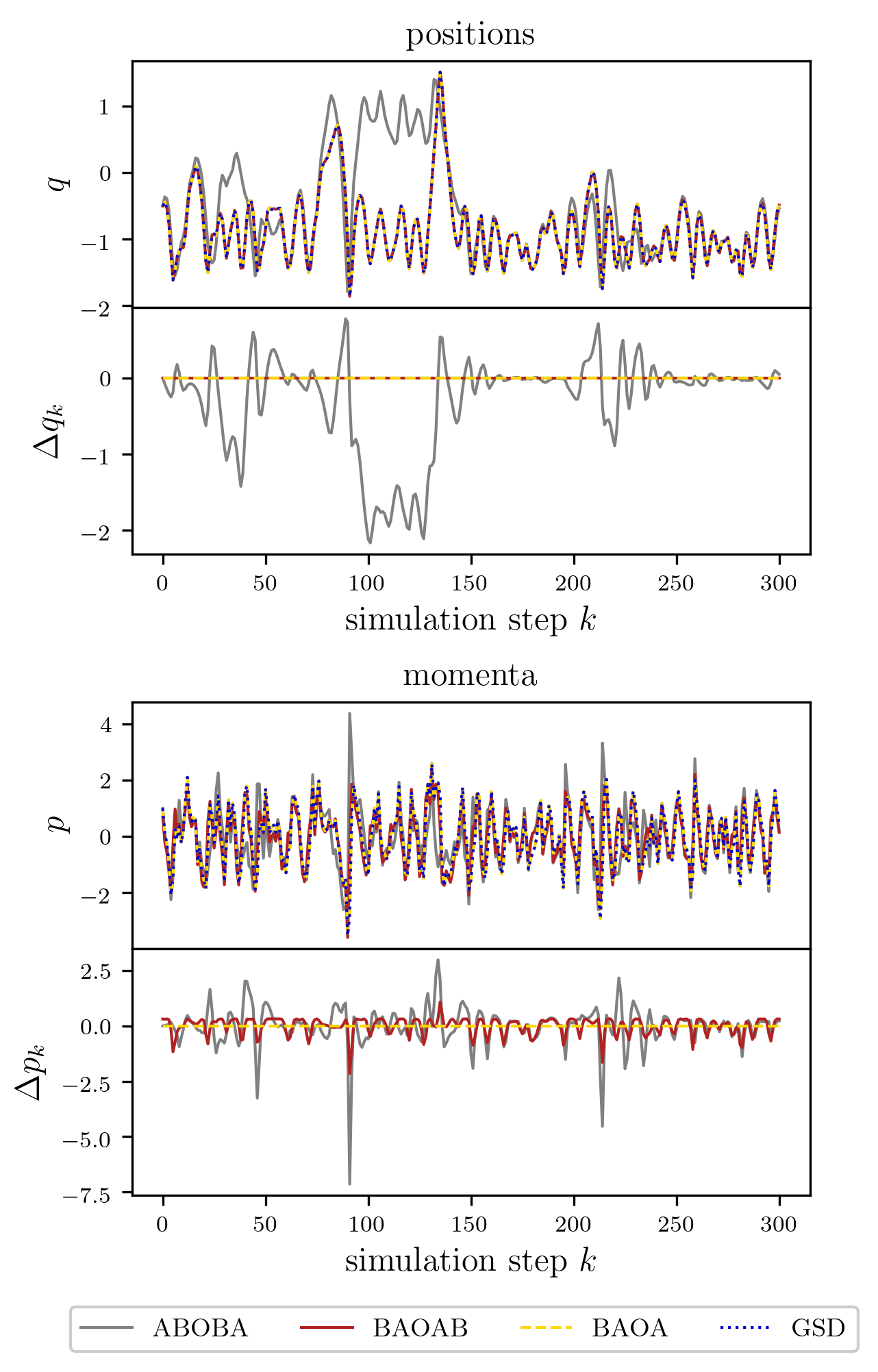
To verify that GSD, BAOA and BAOAB yield the same position trajectories, we calculated example trajectories with these three algorithms. Additionally we included ABOBA Leimkuhler and Matthews 2012; Leimkuhler and Matthews 2013 in the comparison. (See SI section 1 for the algorithm.)

The trajectories were simulated in a one-dimensional tilted double well potential $V(q)=(q^{2}-1)^{2}+q$. To be able to compare the integrators, we generated a sequence of 300 normally distributed random numbers $\bm{\eta}$, and used this $\bm{\eta}$ for the integration with each of the integrators at $\Delta t=0.25$. The initial conditions were $q_{0}=-0.5$ and $p_{0}=1$ for all integratores except BAOAB, for which the intial momentum was adjusted according to eq. 13. (See SI section 2 for all simulation details.)

Fig. 1 shows the position trajectories and the momentum trajectories, as well as the deviations from the GSD trajectory: $\Delta q_{k}^{I}=q_{k}^{\mathrm{GSD}}-q_{k}^{I}$ and $\Delta p_{k}^{I}=p_{k}^{\mathrm{GSD}}-p_{k}^{I}$. The position trajectories of GSD, BAOA and BAOAB are identical. Additionally, the momemtum trajectories of GSD and BAOA are identical, whereas the BAOAB momenta deviate slightly. This confirms our result from sections II.2 and II.3. The ABOBA trajectory deviates in both the positions and the momenta from the GSD/BAOA trajectory.

Note that for a small timestep, the differences between the trajectories of the four integrators are much smaller (SI Fig. 2). This is expected, because all four integrators are guaranteed to converge to the true dynamics for $\Delta t\rightarrow 0$. SI Fig. 3 shows the BAOAB trajectory for $\Delta t=0.25$, if the initial momentum is not adjusted.

Next, we tested whether GSD and BAOA have the same numerical accuracy in the long-time limit. As model systems we use the one-dimensional tilted double-well potential from section III.1 and a box of 1024 TIP3P water molecules Jorgensen et al. 1983. (See SI section 2.)

The left column in Fig. 2 tests how accurately ABOBA, BAOAB, GSD and BAOA reproduce the equilibrium distribution for the 1D potential in position and momentum space with a rather large timestep $\Delta t=0.25$. GSD, BAOA and BAOAB generate the same configurational distribution. Their distribution agrees well with the analytical Boltzmann distribution (SI eq. 4), whereas the distribution generated by ABOBA deviates from the analytical solution. GSD and BAOA yield the same very accurate momentum distribution. (See SI eq. 5 for the analytical Maxwell-Boltzman distribution.) BAOAB underestimates the variance in the momentum distribution leading to a higher peak at $p=0$. Conversely, ABOBA overestimates the variance leading to a lower peak at $p=0$. These results confirm that BAOAB, GSD and BAOA perform equally in configurational sampling while BAOAB differs from GSD and BAOA in momentum space.

The middle column in Fig. 2 reports the accuracy with which the integrators reproduce the target temperature in the 1D potential. We show the relative error $\varepsilon(\Delta t)=(T_{\mathrm{ref}}-T_{\mathrm{approx}}(\Delta t))/T_{\mathrm{ref}}$ as function of the timestep $\Delta t$. Smaller relative errors imply better accuracy. The relative error that is expected for an integrator with second order accuracy, $\varepsilon^{\mathrm{2nd}}=\exp(\Delta t^{2})$, is shown by the dotted line Leimkuhler and Matthews 2013.

The average temperature can either be computed as the configurational temperature $T_{\mathrm{conf}}$, which is an average with respect to the configurational Boltzmann distribution, or as the kinetic temperature $T_{\mathrm{kin}}$, which is an average with respect to the Maxwell-Boltzmann distribution (see SI section 2.A). In accordance with the observation that GSD/BAOA and BAOAB sample the same highly accurate configurational distribution, they also have the same low relative error in $T_{\mathrm{conf}}$. In comparison, ABOBA yields less accurate configurational temperatures with more than 10 % discrepancy for all $\Delta t$. For $T_{\mathrm{kin}}$ the accuracy of GSD/BAOA differs from the accuracy of BAOAB. The relative error in the kinetic temperature sampled by GSD/BAOA is less than 1 % error for any given timestep. BAOAB yields less accurate kinetic temperatures with more than 10 % discrepancy in the $\Delta t>0.23$ regime, similar to the accuracy of ABOBA. This is line with the observation that GSD/BAOA samples the Maxwell-Boltzmann distribution very accurately.

The right column in Fig. 2 shows an accuracy test for a molecular system. Following Ref. Rosta, Buchete, and Hummer 2009 we determined the distributions of the total potential energy and total kinetic energy for bulk TIP3P water Jorgensen et al. 1983 at near-ambient conditions and at two different temperatures, 300 K and 310 K, using a timestep of $\Delta t=2$ fs. As MD software package, we used OpenMM. (See SI section II.B for all simulation details.) We obtain an average potential energy of approximately -9780 kcal/mol at 300 K and -9670 kcal/mol at 310 K which is in good agreement with Ref. Rosta, Buchete, and Hummer 2009. The potential energy distributions of GSD/BAOA and BAOAB are visually indistinguishable for both temperatures, whereas the distribution of ABOBA is shifted to slightly higher potential energies. GSD and BAOA yield kinetic energy distributions whose means agree very well with the average kinetic energy that is expected from the equipartition theorem (dotted lines). (See SI, section 2.B.) The distribution of BAOAB is shifted to lower kinetic energies, which is in line with the underestimated variance of the Maxwell-Boltzmann distribution in the 1D-potential. Conversely, the distribution of ABOBA is slightly shifted to higher kinetic energies.

To check the consistency across different MD software packages, we additionally simulated the TIP3P water box with GROMACSAbraham et al. 2015, i.e. using GSD/BAOA. The results are shown as a green dotted line in Fig. 2. Both, the potential and the kinetic energy distribution, match the results of GSD/BAOA as implemented in OpenMM.

An important property of a Langevin integrator is its ability to provide a single exponential decay in temperature towards the target temperature after a temperature change, The decay rate is called thermal relaxation rate $k_{th}$ and can be adjusted via the friction rate $\xi$. Increasing $\xi$ dampens the term related to the friction force $\exp(-\xi\Delta t)p$ and increase the associated random force term $\sqrt{(1-\exp(-2\xi\Delta t)mk_{B}T}\eta$ in the O-step of the Langevin integrators (e.g. eq. 12c). At high values of $\xi$, fewer simulation steps are necessary to drive the system towards the new target temperature, which corresponds to a high thermal relaxation rate $k_{th}$. At low values of $\xi$, the response to a change in temperature is slow. For an ideal gas with Langevin friction the relation between $k_{th}$ and friction rate $\xi$ is known analytically Goga et al. 2012

(dotted line in Fig. 3). Following Ref. Goga et al. 2012, we determine the thermal relaxation rate $k_{th}$ from simulations of an ideal gas in a cubic box for GSD, BAOA, BAOAB and ABOBA. All four algorithms show the expected first-order decay towards the target temperature. The thermal relaxation rates $k_{th}$ are in good agreement with the analytic solution for all four integrators (Fig. 3). Their standard deviations increase with $\xi$, because at high friction rates the target temperature is reached within few timesteps ($\mathcal{O}(100\,\mathrm{fs})$) which generates a numerical uncertainty in the fit of the decay curve.

References

- Hünenberger (2005) P. H. Hünenberger, “Thermostat algorithms for molecular dynamics simulations,” in Advanced Computer Simulation: Approaches for Soft Matter Sciences I (Springer Berlin Heidelberg, 2005) pp. 105–149.
- Goga et al. (2012) N. Goga, A. Rzepiela, A. De Vries, S. Marrink, and H. Berendsen, “Efficient algorithms for langevin and dpd dynamics,” J. Chem. Theory Comput. 8, 3637–3649 (2012).
- Leimkuhler and Matthews (2012) B. Leimkuhler and C. Matthews, “Rational Construction of Stochastic Numerical Methods for Molecular Sampling,” Appl. Math. Res. eXpress 48, 278 (2012).
- Leimkuhler and Matthews (2013) B. Leimkuhler and C. Matthews, “Robust and efficient configurational molecular sampling via Langevin dynamics,” J. Chem. Phys. 138, 174102 (2013).
- Bussi and Parrinello (2007) G. Bussi and M. Parrinello, “Accurate sampling using Langevin dynamics.” Phys. Rev. E 75, 056707 (2007).
- Abraham et al. (2015) M. J. Abraham, T. Murtola, R. Schulz, S. Páll, J. C. Smith, B. Hess, and E. Lindahl, “Gromacs: High performance molecular simulations through multi-level parallelism from laptops to supercomputers,” SoftwareX 1, 19–25 (2015).
- Thurston, Tovar, and Ferguson (2016) B. A. Thurston, J. D. Tovar, and A. L. Ferguson, “Thermodynamics, morphology, and kinetics of early-stage self-assembly of -conjugated oligopeptides,” Mol. Simul. 42, 955–975 (2016).
- Aldeghi et al. (2017) M. Aldeghi, A. Heifetz, M. J. Bodkin, S. Knapp, and P. C. Biggin, “Predictions of ligand selectivity from absolute binding free energy calculations,” J. Am. Chem. Soc. 139, 946–957 (2017).
- Mansbach et al. (2021) R. A. Mansbach, S. Chakraborty, K. Nguyen, D. C. Montefiori, B. Korber, and S. Gnanakaran, “The sars-cov-2 spike variant d614g favors an open conformational state,” Sci. Adv. 7, eabf3671 (2021).
- Marrink and Tieleman (2013) S. J. Marrink and D. P. Tieleman, “Perspective on the martini model,” Chem. Soc. Rev. 42, 6801–6822 (2013).
- Goga et al. (2015) N. Goga, M. Melo, A. Rzepiela, A. De Vries, A. Hadar, S. Marrink, and H. Berendsen, “Benchmark of schemes for multiscale molecular dynamics simulations,” J. Chem. Theory Comput. 11, 1389–1398 (2015).
- Deichmann et al. (2018) G. Deichmann, M. Dallavalle, D. Rosenberger, and N. F. van der Vegt, “Phase equilibria modeling with systematically coarse-grained models—a comparative study on state point transferability,” J. Phys. Chem. B 123, 504–515 (2018).
- Pezeshkian et al. (2020) W. Pezeshkian, M. König, T. A. Wassenaar, and S. J. Marrink, “Backmapping triangulated surfaces to coarse-grained membrane models,” Nat. Commun. 11, 1–9 (2020).
- Goicochea et al. (2015) A. G. Goicochea, M. B. Altamirano, J. Hernández, and E. Pérez, “The role of the dissipative and random forces in the calculation of the pressure of simple fluids with dissipative particle dynamics,” Comput. Phys. Commun. 188, 76–81 (2015).
- Moga et al. (2013) S. Moga, G. Dragoi, A. Hadar, and N. Goga, “A parallelization scheme for new dpd-b thermostats,” J. At. Mol. Phys. 2013 (2013).
- Schneider et al. (2017) J. Schneider, J. Hamaekers, S. T. Chill, S. Smidstrup, J. Bulin, R. Thesen, A. Blom, and K. Stokbro, “Atk-forcefield: a new generation molecular dynamics software package,” Model. Simul. Mater. Sci. Eng. 25, 085007 (2017).
- Jung, Okazaki, and Hummer (2017) H. Jung, K.-i. Okazaki, and G. Hummer, “Transition path sampling of rare events by shooting from the top,” J. Chem. Phys. 147, 152716 (2017).
- Moga et al. (2015) A. Moga, I. Marin, N. Goga, A. Hadar, D. Geroge, and K. Oluwatoyin, “Improved openmm algorithms for cuda and opencl using new stochastic dynamics and the berendsen thermostat,” in 2015 6th International Conference on Computing, Communication and Networking Technologies (ICCCNT) (IEEE, 2015) pp. 1–6.
- Madeo et al. (2020) D. Madeo, G. Bevilacqua, V. Biancalana, Y. Dancheva, and C. Mocenni, “A physical model for the characterization of magnetic hydrogels subject to external magnetic fields,” J. Magn. Magn. Mater 493, 165674 (2020).
- ope (2022) “OpenMMTools Github,” https://github.com/choderalab/openmmtools (accessed: 07.02.2022).
- Fass et al. (2018) J. Fass, D. A. Sivak, G. E. Crooks, K. A. Beauchamp, B. Leimkuhler, and J. D. Chodera, “Quantifying Configuration-Sampling Error in Langevin Simulations of Complex Molecular Systems,” Entropy 20, 318 (2018).
- Eastman et al. (2017) P. Eastman, J. Swails, J. D. Chodera, R. T. McGibbon, Y. Zhao, K. A. Beauchamp, L.-P. Wang, A. C. Simmonett, M. P. Harrigan, C. D. Stern, R. P. Wiewiora, B. R. Brooks, and V. S. Pande, “Openmm 7: Rapid development of high performance algorithms for molecular dynamics,” PLOS Computat. Biol. 13, 1 (2017).
- Brotzakis and Bolhuis (2019) Z. F. Brotzakis and P. G. Bolhuis, “Approximating free energy and committor landscapes in standard transition path sampling using virtual interface exchange,” J. Chem. Phys. 151, 174111 (2019).
- Starr et al. (2021) T. N. Starr, N. Czudnochowski, Z. Liu, F. Zatta, Y.-J. Park, A. Addetia, D. Pinto, M. Beltramello, P. Hernandez, A. J. Greaney, R. Marzi, W. G. Glass, I. Zhang, A. S. Dingens, J. E. Bowen, M. A. Tortorici, A. C. Walls, J. A. Wojcechowskyj, A. De Marco, L. E. Rosen, J. Zhou, M. Montiel-Ruiz, H. Kaiser, J. R. Dillen, H. Tucker, J. Bassi, C. Silacci-Fregni, M. P. Housley, J. di Iulio, G. Lombardo, M. Agostini, N. Sprugasci, K. Culap, S. Jaconi, M. Meury, E. Dellota Jr, R. Abdelnabi, S.-Y. C. Foo, E. Cameroni, S. Stumpf, T. I. Croll, J. C. Nix, C. Havenar-Daughton, L. Piccoli, F. Benigni, J. Neyts, A. Telenti, F. A. Lempp, M. S. Pizzuto, J. D. Chodera, C. M. Hebner, H. W. Virgin, S. P. J. Whelan, D. Veesler, D. Corti, J. D. Bloom, and G. Snell, “Sars-cov-2 rbd antibodies that maximize breadth and resistance to escape,” Nature 597, 97–102 (2021).
- Sivak, Chodera, and Crooks (2013) D. A. Sivak, J. D. Chodera, and G. E. Crooks, “Using nonequilibrium fluctuation theorems to understand and correct errors in equilibrium and nonequilibrium simulations of discrete langevin dynamics,” Phys. Rev. X 3, 011007 (2013).
- Baczewski and Bond (2013) A. D. Baczewski and S. D. Bond, “Numerical integration of the extended variable generalized langevin equation with a positive prony representable memory kernel,” J. Chem. Phys. 139, 044107 (2013).
- Plé et al. (2019) T. Plé, S. Huppert, F. Finocchi, P. Depondt, and S. Bonella, “Sampling the thermal wigner density via a generalized langevin dynamics,” J. Chem. Phys. 151, 114114 (2019).
- Duong and Shang (2021) M. H. Duong and X. Shang, “Accurate and robust splitting methods for the generalized langevin equation with a positive prony series memory kernel,” arXiv preprint arXiv:2109.07879 (2021).
- Liu, Li, and Liu (2016) J. Liu, D. Li, and X. Liu, “A simple and accurate algorithm for path integral molecular dynamics with the langevin thermostat,” J. Chem. Phys. 145, 024103 (2016).
- Lopanitsyna, Mahmoud, and Ceriotti (2021) N. Lopanitsyna, C. B. Mahmoud, and M. Ceriotti, “Finite-temperature materials modeling from the quantum nuclei to the hot electron regime,” Phys. Rev.Mater. 5, 043802 (2021).
- Leimkuhler, Margul, and Tuckerman (2013) B. Leimkuhler, D. T. Margul, and M. E. Tuckerman, “Stochastic, resonance-free multiple time-step algorithm for molecular dynamics with very large time steps,” Mol. Phys. 111, 3579–3594 (2013).
- Lagardère, Aviat, and Piquemal (2019) L. Lagardère, F. Aviat, and J.-P. Piquemal, “Pushing the limits of multiple-time-step strategies for polarizable point dipole molecular dynamics,” J. Phys. Chem. Lett. 10, 2593–2599 (2019).
- Sivak, Chodera, and Crooks (2014) D. A. Sivak, J. D. Chodera, and G. E. Crooks, “Time step rescaling recovers continuous-time dynamical properties for discrete-time langevin integration of nonequilibrium systems.” J. Phys. Chem. B 118, 6466–6474 (2014).
- Leimkuhler and Matthews (2016a) B. Leimkuhler and C. Matthews, Molecular Dynamics. (Springer, 2016).
- Bou-Rabee and Owhadi (2010) N. Bou-Rabee and H. Owhadi, “Long-run accuracy of variational integrators in the stochastic context,” SIAM J. Numer. Anal. 48, 278–297 (2010).
- Zhang et al. (2019) Z. Zhang, X. Liu, K. Yan, M. E. Tuckerman, and J. Liu, “Unified efficient thermostat scheme for the canonical ensemble with holonomic or isokinetic constraints via molecular dynamics,” J. Phys. Chem. A 123, 6056–6079 (2019).
- Song and Tan (2021) Z. Song and Z. Tan, “On irreversible metropolis sampling related to langevin dynamics,” arXiv preprint arXiv:2106.03012 (2021).
- Case et al. (2021) D. A. Case, H. M. Aktulga, K. Belfon, I. Ben-Shalom, S. R. Brozell, D. S. Cerutti, T. E. Cheatham III, V. W. D. Cruzeiro, T. A. Darden, R. E. Duke, et al., Amber 2021 (University of California, San Francisco, 2021).
- Jorgensen et al. (1983) W. L. Jorgensen, J. Chandrasekhar, J. D. Madura, R. W. Impey, and M. L. Klein, “Comparison of simple potential functions for simulating liquid water,” J. Chem. Phys. 79, 926–935 (1983).
- Rosta, Buchete, and Hummer (2009) E. Rosta, N.-V. Buchete, and G. Hummer, “Thermostat artifacts in replica exchange molecular dynamics simulations,” J. Chem. Theory Comput. 5, 1393–1399 (2009).
- Grønbech-Jensen and Farago (2013) N. Grønbech-Jensen and O. Farago, “A simple and effective verlet-type algorithm for simulating langevin dynamics,” Mol. Phys. 111, 983–991 (2013).
- Li et al. (2017) D. Li, X. Han, Y. Chai, C. Wang, Z. Zhang, Z. Chen, J. Liu, and J. Shao, “Stationary state distribution and efficiency analysis of the langevin equation via real or virtual dynamics,” The Journal of Chemical Physics 147, 184104 (2017).
- Finkelstein et al. (2021) J. Finkelstein, C. Cheng, G. Fiorin, B. Seibold, and N. Grønbech-Jensen, “Bringing discrete-time langevin splitting methods into agreement with thermodynamics,” The Journal of Chemical Physics 155, 184104 (2021).
- Ope (2022) “Documentation of the openmm python api: Langevinmiddleintegrator,” http://docs.openmm.org/development/api-python/generated/openmm.openmm.LangevinMiddleIntegrator.html (2015 (accessed: 30.03.2022)).
- AMB (2022) “Amber 2021 reference manual, section 21.6.10.” https://ambermd.org/doc12/Amber21.pdf (2021 (accessed: 26.05.2022)).
- Leimkuhler, Matthews, and Stoltz (2016) B. Leimkuhler, C. Matthews, and G. Stoltz, “The computation of averages from equilibrium and nonequilibrium langevin molecular dynamics,” IMA Journal of Numerical Analysis 36, 13–79 (2016).
- Peters, Goga, and Berendsen (2014) E. J. F. Peters, N. Goga, and H. J. Berendsen, “Stochastic dynamics with correct sampling for constrained systems,” J. Chem. Theory Comput. 10, 4208–4220 (2014).
- Leimkuhler and Matthews (2016b) B. Leimkuhler and C. Matthews, “Efficient molecular dynamics using geodesic integration and solvent–solute splitting,” Proc. R. Soc. A: Math. Phys. Eng. Sci. 472, 20160138 (2016b).
- Donati, Hartmann, and Keller (2017) L. Donati, C. Hartmann, and B. G. Keller, “Girsanov reweighting for path ensembles and markov state models,” J. Chem. Phys. 146, 244112 (2017).
- Donati and Keller (2018) L. Donati and B. G. Keller, “Girsanov reweighting for metadynamics simulations,” J. Chem. Phys. 149, 072335 (2018).
- Kieninger and Keller (2021) S. Kieninger and B. G. Keller, “Path probability ratios for langevin dynamics—exact and approximate,” J. Chem. Phys. 154, 094102 (2021).
- Git (2022) “Github repository bkellerlab/gsd_baoa_baoab,” https://github.com/bkellerlab/GSD_BAOA_BAOAB (2022 (accessed: 26.05.2022)).