Inexact reduced gradient methods
in nonconvex optimization
Abstract. This paper proposes and develops new linesearch methods with inexact gradient information for finding stationary points of nonconvex continuously differentiable functions on finite-dimensional spaces. Some abstract convergence results for a broad class of linesearch methods are established. A general scheme for inexact reduced gradient (IRG) methods is proposed, where the errors in the gradient approximation automatically adapt with the magnitudes of the exact gradients. The sequences of iterations are shown to obtain stationary accumulation points when different stepsize selections are employed. Convergence results with constructive convergence rates for the developed IRG methods are established under the Kurdyka-Łojasiewicz property. The obtained results for the IRG methods are confirmed by encouraging numerical experiments, which demonstrate advantages of automatically controlled errors in IRG methods over other frequently used error selections.
Key words: Nonconvex optimization, inexact reduced gradient methods, linesearch methods, Kurdyka-Łojasiewicz property, convergence rates
Mathematics Subject Classification (2020) 90C30, 90C52, 49M05
1 Introduction
Consider the unconstrained optimization problem formulated as follows:
| (1.1) |
with a continuously differentiable (-smooth) objective function . One of the most natural and classical approaches to solve (1.1) is by using linesearch methods; see, e.g., [8, 10, 27, 42, 44, 47]. Given a starting point , such methods construct the iterative procedure
| (1.2) |
where is a stepsize at the iteration, and where the direction satisfies the condition
The classical choice for the direction is when the resulting algorithm is known as the gradient descent method; see the aforementioned books and the references therein. If is twice continuously differentiable (-smooth) and the Hessian matrix is positive-definite, then is chosen by solving the linear equation
and it is known as a Newton direction [10, 24, 27]. Additionally, more general choices of descent directions widely used are the gradient related directions [10, Page 41], directions satisfying an angle condition [1, Page 541], etc. Together with the descent directions, stepsizes are usually chosen to ensure the decreasing property of the entire sequence or sometimes only its tail. Well-known stepsize selections are constant stepsize, diminishing stepsize (not summable), stepsizes following Armijo rule, and Wolfe conditions; see, e.g., [1, 8, 10, 27, 42, 44, 47].
The stationarity of accumulation points generated by linesearch methods with gradient related directions and stepsizes following the Armijo rule is established in [10, Proposition 1.2.1]. When the Lipschitz continuity of the gradient is additionally assumed, the same type of convergence is achieved if either the stepsize is constant and directions are gradient related, or the stepsize is diminishing and directions satisfy more involved conditions [10, Proposition 1.2.3]. The global convergence of some linesearch methods to an isolated stationary point relies on the Ostrowski condition; see [45] and [24, Theorem 8.3.9]. If there is no guarantee on the isolation of stationary points, algebraic geometry tools introduced by Łojasiewicz [37] and Kurdyka [34] are used for linesearch methods with directions satisfying the angle conditions and the stepsize following the Wolfe conditions; see [1, Theorem 4.1]. While rates of convergence of general linesearch methods are not considered, some specific methods achieve certain convergence rates for particular classes of functions. For instance, the gradient descent method achieves a local linear rate of convergence if the objective function is twice differentiable with Lipschitz continuous Hessian as in [42, Theorem 1.2.4], and the (generalized) damped Newton method attains a superlinear convergence rate of under the positive-definiteness of the (generalized) Hessian and some additional assumptions; [30, Theorem 4.5]. Furthermore, a linear rate of convergence for the gradient descent method is achieved under either the Polyak-Łojasiewicz condition as in [46] and [29], or under the weak convexity of the objective function as in [50].
Due to its simplicity, the gradient descent method is broadly used to solve various optimization problems; see, e.g., [14, 19, 20, 43, 51]. However, errors in gradient calculations may appear in many situations, which can be found in practical problems arising, e.g., in the design of space trajectories [2] and computer-aided design of microwave devices [25]. Moreover, many nonsmooth optimization problems can be transformed into its smoothed versions by using Moreau envelopes [49] and forward-backward envelopes [52]. Nevertheless, gradients of smoothed functions cannot be usually computed precisely, and therefore various gradient methods with inexact gradient information have been suggested. We mention the following major developments in this vein:
- •
- •
Gilmore and Kelley [25] propose an implicit filtering algorithm to deal with certain box constrained optimization problems, where the objective function is a sum of a -smooth function with Lipschitz continuous gradient and a noise function.
- •
Bertsekas shows in [10, pp. 44–45] that if the objective function is -smooth with a Lipschitz continuous gradient and if the error of inexact gradient is either small relative to the norm of the exact gradient, or proportional to the stepsize, then convergence behavior of gradient methods is similar to the case where there are no errors.
All the convergence results for inexact gradient methods mentioned above assume that the objective function is either -smooth with a Lipschitz continuous gradient, or convex. To the best of our knowledge, general methods of solving nonconvex -smooth optimization problems with inexact information on non-Lipschitzian gradients are not available in the literature. One of the reasons for this is that verifying the descent property of the sequence of function values without the Lipschitz continuity of via the Armijo linesearch requires exact information on gradients. To deal with inexactness, we need a descent direction that allows us to replace the Armijo linesearch procedure by another one not demanding exact gradients. In addition, a practical inexact gradient method that uses constant stepsize for a general nonconvex -smooth function with the Lipschitz gradient is also not established. Although an inexact gradient method with constant stepsize is proposed in [10, pp. 44–45] by using an error smaller than the norm of the exact gradient, the problem of how to control this error while the exact gradient is unknown is still questionable.
Having in mind the above discussion, we introduce new inexact reduced gradient (IRG) methods to find stationary points for a general class of nonconvex -smooth functions. Although our proposed methods address smooth problems, some motivations for them partly come from a certain nonsmooth algorithm and generalized differential tools of variational analysis. Specifically, to find a Clarke stationary point of a nonsmooth locally Lipschitzian function, the gradient sampling (GS) method, introduced by Burke et al. [16] and modified by Kiwiel [32], approximates at each iteration the -generalized gradient by the convex hull of nearby gradients. In the GS method, the negative projection of the origin onto this convex hull is chosen as the descent direction and the stepsizes are chosen from the backtracking linesearch as in [32, Section 4.1]. Although the GS method work well for nonsmooth problems, using them for smooth functions seems to be challenging due to, in particular, the necessity to solve subproblems of finding projections onto convex hulls. However, replacing the -generalized gradient by the Fréchet-type -subdifferential makes our methods much simpler and suitable for smooth problems. Indeed, the latter construction for a -smooth function at the point in question is just the closed ball centered at its gradient with radius . Thus the projection of the origin onto this ball has an explicit and simple form. The descent direction chosen by this projection also allows us to replace the exact gradient by its approximation and to use a linesearch procedure that does not require exact gradients. Developing this idea, we design our inexact reduced gradient methods with non-normalized directions together with some stepsize selections such as backtracking stepsize, constant stepsize, and diminishing stepsize. To the best of our knowledge, the IRG methods that we propose and develop in this paper are completely new even in the exact case. It should also be emphasized that the proposed IRG methods are not special versions of the GS one since the latter needs exact gradients at multiple points in each iteration, while the IRG methods need only one inexact gradient. Moreover, the iterative sequence of the GS method is chosen randomly while IRG iterations are designed deterministically. Our main results include the following:
- •
Designing a general framework for the IRG methods and revealing their basic properties.
- •
Finding stationary accumulation points of iterations in the IRG methods with backtracking stepsizes as well as with either constant stepsizes, or diminishing ones under an additional descent condition on the objective functions.
- •
Obtaining the global convergence of iterations in the IRG methods with constructive convergence rates depending on the exponent of the imposed Kurdyka-Łojasiewicz property of the objective functions.
These results are achieved by using our newly developed scheme for general linesearch methods described in the following way. To begin with, some conditions are proposed to ensure the stationary of accumulation points in general linesearch methods. If the KL property is additionally assumed, then the global convergence of the iterative sequence to a stationary point is guaranteed. Moreover, the rates of convergence are established if the stepsize is bounded away from zero.
From a practical viewpoint, our IRG methods automatically adjust the errors required for finding approximate gradients, which will be shown to have numerical advantages over decreasing errors, e.g., as , that are frequently used in the existing methods [10, 22, 25]. To elaborate more on this issue, observe that since the magnitude of the exact gradient is small near the stationary points and is larger elsewhere, decreasing errors that do not take the information of the exact or inexact gradients into consideration may encounter the following phenomena:
- •
Over approximation, which happens when the magnitude of the exact gradient is large but the error is too small. In this case, the procedures of finding approximate gradient may execute longer than needed to obtain a good approximation of the exact gradient.
- •
Under approximation, which happens when the magnitude of the exact gradient is small but the error is too large, which may lead us to an approximate gradient that is not good enough. As a consequence of using such an approximate gradient, the next iterative element can be worse instead of being better than the current one.
In contrast to methods using decreasing errors, our IRG methods, by performing a low cost checking step in each iteration to determine whether the error for the approximation procedure should be decrease or stay the same in the next iteration, use errors which automatically adapt with the magnitudes of the exact gradients to avoid the aforementioned phenomena and exhibit a better performance.
The rest of the paper is organized as follows. Section 2 discusses basic notions related to methods. Some abstract convergence results for linesearch methods are established in Section 3. In Section 4, we introduce a general form of the IRG methods and investigate their principal properties. Our main results about the convergence behavior of the IRG methods with different stepsize selections are given in Section 5. The numerical experiments conducted in Section 6 support the theoretical results obtained in Section 5 and show that the IRG methods with the new type of automatically controlled errors have a better performance in comparison with the inexact proximal point method in the Least Absolute Deviations Curve-Fitting problem taken from [11]. In Section 6, we also compare numerically the performance of our IRG methods with those of the reduced gradient method and the gradient decent method employing the exact gradient calculations for two well-known benchmark functions in global optimization. The last Section 7 discusses some directions of our future research.
2 Linesearch Methods and Related Properties
First we recall some notions and notation frequently used in what follows. All our considerations are given in the space with the Euclidean norm and scalar/inner product . We use , , and to denote the collections of natural numbers, positive numbers, and the extended real line, respectively. The symbol means that as with . For a -smooth function , is a stationary point of if . The function is said to satisfy the -descent condition with some if
| (2.1) |
We see that -descent condition (2.1) means that the graphs o the quadratic functions lie above that of for all This condition is equivalent to the convexity of [53, Lemma 4], while being a direct consequence of the -Lipschitz continuity of , i.e., the Lipschitz continuity of with constant ; see, e.g., [10, Proposition A.24] and [27, Lemma A.11]. The converse implication holds when is convex [6, 53] but fails otherwise. A major class of real-valued functions satisfying the -descent condition but not having the Lipschitz continuous gradient is given by
where is an matrix, , and is a smooth convex function whose gradient is not Lipschitz continuous, e.g., , where is an matrix and Indeed, we can find some such that the matrix is positive-semidefinite, where is the identity matrix. It follows from the second-order characterization of convex functions that
Combining this with the convexity of , we get the convexity of which means that satisfies the descent property (2.1).
Even when is Lipschitz continuous with constant , can satisfy the descent condition with . E.g., consider the univariate function together with its gradient given by
The latter representation implies that is the smallest constant for the Lipschitz continuity of . Meanwhile, we see on Figure 1 that satisfies the -descent property with

Next we recall by following [10, Section 1.2] some basic stepsize selections for the iterative procedure (1.2). The stepsize sequence satisfies the Armijo rule if there exist a scalar and a reduction factor such that for all we have the representation
| (2.2) |
This stepsize selection ensures the nonincreasing property of the entire sequence . However, Armijo stepsizes may be small and thus require a large number of stepsize reducing steps in order to make just small changes of the iterative sequence.
To significantly simplify the iterative sequence design, it is possible to consider a constant stepsize, i.e., for all . For this rule, the nonincreasing property of is not ensured in general but holds under the -descent condition (2.1) whenever is chosen to be sufficiently small with respect to , see, e.g., [10, 44]. However, even when the -descent condition is satisfied for while an approximate value of is unknown, using constant stepsizes becomes inefficient. In such a case, it is possible to use the diminishing stepsize selection, i.e.,
| (2.3) |
Drawbacks of the latter selection are the eventual slow convergence due to its small stepsizes and the absence of the descent property for the iterative sequence .
Now we formulate a general type of directions that plays a crucial role in our subsequent analysis of various linesearch methods.
Definition 2.1.
Let be a sequence in . The direction sequence is called gradient associated with if we have the implication
| (2.4) |
It can be easily checked that if either
| (2.5) |
or there exists some constant such that
| (2.6) |
then is gradient associated with . Many methods such as the gradient descent, the generalized damped Newton method [30, 31], and the methods appeared in [10, Proposition 1.2.3] satisfy (2.6), while (2.5) can be considered as a standard condition for inexact gradient directions. It should be also mentioned that the notion of gradient associated directions is different from the notion of gradient related directions proposed by Bertsekas in [10].
Finally in this section, we discuss two versions of the fundamental KL property playing plays a crucial role in the results on global convergence and convergence rates established in what follows. The first version, which is mainly used in the paper, is due to Absil et al. [1, Theorem 3.4].
Definition 2.2.
Let be a differentiable function. We say that satisfies the KL property at if there exist a number , a neighborhood of , and a nondecreasing function such that the function is integrable over and we have
| (2.7) |
for all with .
Remark 2.3.
For smooth functions , the KL property from Definition 2.2 is weaker than the KL property of at introduced by Attouch et al. in [5] meaning that there exist a number , a neighborhood of , and a continuous concave function such that
- (i)
;
- (ii)
is -smooth on ;
- (iii)
on ;
- (iv)
for all with , we have
(2.8)
Supposing that satisfies the KL property at in the sense of Attouch et al., we now show that it satisfies the KL property from Definition 2.2. Indeed, take , and the function satisfying conditions (i)-(iv) in Remark 2.3. By (iii), the function given by
is well-defined. Since is concave, is nonincreasing. Therefore, is a nondecreasing positive function that is integrable on . Moreover, by we get that (2.8) and (2.7) are equivalent. Thus satisfies the KL property at in the sense of Definition 2.2.
It has been realized that KL property in the sense of Attouch et al., and hence the one from Definition 2.2, is satisfied in broad settings. In particular, it holds at every nonstationary point of ; see [5, Lemma 2.1 and Remark 3.2(b)]. Furthermore, it is proved at the original paper by Łojasiewicz [37] that any analytic function satisfies the KL property at every point with for some . Typical smooth functions satisfying this property are semialgebraic functions and also those from the more general class of functions definable in o-minimal structures; see [12, 34]. For other examples of functions satisfying the KL property, we refer the reader to [5, 35] and the bibliographies therein.
3 Abstract Convergence Results for Linesearch Methods
In this section, we establish properties for a general class of linesearch methods of type (1.2), which provide major tools for convergence analysis of IRG methods in Section 5. One of the most important results desired for linesearch methods is as follows:
| (3.1) |
By the continuity of the gradient mapping, the desired property (3.1) automatically holds if for each accumulation point of we can find an infinite set such that and . If the exact information on the gradient is unknown while is gradient associated with , i.e., (2.4) is satisfied, then property (3.1) is satisfied when
| (3.2) |
We are going to show that (3.2) holds whenever is an accumulation point of and
| (3.3) |
The following lemma is new and is crucial in the convergence analysis for many linesearch methods.
Lemma 3.1.
Let and be sequences satisfying (3.3). If is an accumulation point of and if is an accumulation point of , then there exists an infinite set such that
| (3.4) |
[Proof.] If as , the conclusion obviously holds, so suppose that . It suffices to show that for any sufficiently small and any there is a number such that
Fix such and . Since is sufficiently small and , suppose that the set
As is an accumulation point of and is an accumulation point of , we get that
It suffices to verify that Suppose on the contrary that , i.e.,
By (3.3), we have the estimates
which ensure the series convergence
| (3.5) |
Taking any number , we also have Since is infinite and form a partition of the set including , there exists a number with such that . Then we have the estimates
Using the triangle inequality and (3.5) gives us
which brings us to a contradiction that completes the proof of the lemma.
Remark 3.2.
Our proof of Lemma 3.1 is inspired by the proofs of Kiwiel in [32, Theorem 3.3(iii)], [33, Theorem 3.8(iii)] and of Burke and Lin in [17, Theorem 5]. If is not an accumulation point of , then (3.3) implies that is convergent. Indeed, the negation of the statement that is an accumulation point of yields the existence of and such that
It follows from (3.3) that
which implies that is a Cauchy sequence, and thus it converges.
Next we recall classical results that describe important properties of the set of accumulation points generated by a sequence satisfying a limit condition introduced by Ostrowski; see (3.6) below. The result from Lemma 3.3(i) was first established in [45, Theorem 28.1], while assertion (ii) of this lemma appeared in [23]. These results are also stated as Theorem 8.3.9 and Theorem 8.3.10 in the book of Facchinei and Pang [24]. More recent usage of the of the Ostrowski condition in the framework of linesearch methods can be found in [13, Lemma 5(iii)].
Lemma 3.3.
Let be a sequence satisfying the Ostrowski condition
| (3.6) |
Then the following assertions hold:
- (i)
If is bounded, then the set of accumulation points of is nonempty, compact, and connected in .
- (ii)
If has an isolated accumulation point, then this sequence converges to it.
Now we are ready to establish the main result of this section revealing major convergence properties of a general class of linesearch methods.
Theorem 3.4.
Let be a sequence generated by a linesearch method (1.2) such that:
- (a)
is gradient associated with ;
- (b)
is an accumulation point of
- (c)
Then every accumulation point of is a stationary point of . Moreover, if is bounded from above, then the following assertions hold:
- (i)
If is bounded, then the set of accumulation points of is nonempty, compact, and connected.
- (ii)
If has an isolated accumulation point, then this sequence converges to it.
[Proof.] Let be an accumulation point of . Note that (c) is equivalent to (3.3) under the linesearch relationship in (1.2). Applying Lemma 3.1 with taking into account (b) and (c), we can find an infinite set such that and . Then (a) implies that . Employing the continuity of , we have
which tells us that is a stationary point of . Suppose now that is bounded from above by some . Using (c), we immediately get
This leads us to and verifies assertions (i) and (ii) by applying Lemma 3.3.
Theorem 3.4 also allows us to ensure the stationarity of accumulation points generated by linesearch methods (1.2) applied to functions satisfying the -descent condition (2.1), where the stepsize is either constant or diminishing, and where the direction is gradient associated while satisfying the following sufficient descent condition
| (3.7) |
with some constant . Note that condition (3.7) is different from the gradient associated condition from Definition 2.1, since from (3.7) we only have that yields but the reverse implication may not hold. In addition to the gradient descent and generalized Newton methods discussed above, there exist many other linesearch methods using direction (3.7); e.g., the boosted difference of convex functions algorithm as in [3, Proposition 4]), the inexact Levenberg-Marquardt method as in [21, Algorithm 3.1]), and the GS method for nonsmooth functions with non-normalized direction given in [32, Section 4.1].
We have the following effective consequence of Theorem 3.4.
Corollary 3.5.
Let be a sequence generated by a linesearch method (1.2). Suppose that , and that we have the conditions:
- (a)
satisfies the -descent condition (2.1) for some ;
- (b)
the sequence is gradient associated with and satisfies (3.7) for some
- (c)
the sequence is not summable, i.e.,
(3.8) and there are numbers and such that
(3.9)
Then every accumulation point of is stationary for , and the following assertions hold:
- (i)
If the sequence is bounded, then the collection of accumulation points of is nonempty, compact, and connected.
- (ii)
If has an isolated accumulation point, then the entire sequence converges to it.
Moreover, if is bounded away from then as .
[Proof.] It follows from (3.9) in condition (c) that
Since satisfies -descent condition (2.1), we deduce from (3.7) and the latter inequality that
| (3.10) |
Then summing up the relationships over and using the assumption give us
| (3.11) |
Now we show that is an accumulation point of . Suppose on the contrary that there exist a positive number and a natural number such that
Using this together with (3.11) imply that , which contradicts (3.8). Therefore, is an accumulation point of . Combining the latter with (b), (3.11), and (3.9) allows us to confirm that all the assumptions of Theorem 3.4 are satisfied. Thus every accumulation point of is a stationary point of , and both assertions in (i) and (ii) hold.
If finally is bounded away from it follows from (3.11) that as . Since the sequence is gradient associated with by (b), we get .
Remark 3.6.
Let us compare Corollary 3.5 with two well-known results by Bertsekas [10] about the convergence of linesearch methods. First we compare the result of Corollary 3.5 in the case where is bounded away from with Bertsekas’s result for the constant stepsize.
Proposition 3.7.
[10, Proposition 1.2.2] Let be a sequence generated by a linesearch method , where the sequence is gradient related. Assume that
| (3.12) |
with some constant , and that for all we have and
| (3.13) |
where is a fixed positive scalar, and where
Then every limit point of is a stationary point of .
Our comparison with this result are as follows:
- 1.
- 2.
Regarding the stepsize selection, our choice is much simpler than the one used in [10, Proposition 1.2.2]. Observe that in the direction selection, we use as gradient associated with and satisfying the sufficient descent condition, while [10, Proposition 1.2.2] used the gradient related direction. It is commented in the note after [10, Proposition 1.2.2] that if the direction is chosen better, i.e., there are two numbers satisfying
(3.14) then the stepsize selection can be reduced to the one chosen above. It can be seen that (3.14) yields the estimates
and for any infinite set we have if and only if . Therefore, condition (b) in Corollary 3.5 and the gradient related condition share the common direction (3.14).
- 3.
Comparing the conclusions of Corollary 3.5 and of [10, Proposition 1.2.2], observe that our result establishes the convergence to of the entire sequence , which is stronger than the stationarity of accumulation points obtained by [10, Proposition 1.2.2]. Moreover, our results about the set of accumulation points and convergence to an isolated accumulation point by using the Ostrowski condition are not given in [10, Proposition 1.2.2].
Next we compare the usage of the diminishing stepsize in Corollary 3.5 with the the corresponding result by Bertsekas [10].
Proposition 3.8.
[10, Proposition 1.2.3] Let be a sequence generated by a linesearch method . Assume that is -Lipschitzian, and that there exist positive scalars such that (3.14) holds for all . Suppose also that
| (3.15) |
Then either , or converges to a finite value with as . Furthermore, every accumulation point of is a stationary point of .
Here are our comparison with the latter proposition.
- 1.
The -Lipschitz continuity of yields -descent condition while the converse implication fails; see the commentaries in Section 2. The convergence of to is the main result of [10, Proposition 1.2.3], and technically it cannot be derived without the -Lipschitz continuity of or its small modifications. Relaxing the Lipschitz continuity of the gradient to the descent condition may allow us to work with broader classes of functions by replacing the usual Euclidean distance by the Bregman distance; see, e.g., [6, 15, 38].
- 2.
- 3.
- 4.
To summarize, if considering the stationarity of accumulation points only, Corollary 3.5 covers [10, Proposition 1.2.3] with a larger class of objective functions as well as descent directions. On the other hand, the convergence of to is not obtained in Corollary 3.5 since the -Lipschitz continuity is relaxed therein.
Next we present the convergence result for linesearch methods under the fulfillment of the KL property, which is taken from [1, Theorem 3.4].
Proposition 3.9.
Let be a -smooth function, and let the sequence of iterations satisfy the following conditions:
- (H1)
(primary descent condition). There exists such that for sufficiently large we have
- (H2)
(complementary descent condition). For sufficiently large , we have
If is an accumulation point of and satisfies the KL property at , then as .
Note that [1, Theorem 3.2] provides a detailed proof for Proposition 3.9 when satisfies the KL property at with for some and . The key ingredient of the proof is the existence of some such that
| (3.16) |
Using this, we can deduce that
| (3.17) |
and so the sequence is convergent.
Next we address rates of convergence of linesearch methods of type (1.2). Finding convergence rates for the gradient descent method in nonconvex settings is an important issue that has received an increasing attention recently; see, e.g., [29, 50] and the references therein. Our results in Theorem 3.11 establish the rate of convergence of general linesearch methods under the KL property and the boundedness of stepsizes away from . The proof below employs the technique developed in the proof of [4, Theorem 2] for the proximal point method. This technique is also used in the proofs of convergence rates for the difference of convex algorithm [36] and its boosted version in [3, Theorem 1]. The next technical lemma taken from [3, Lemma 1] is needed in what follows.
Lemma 3.10.
Let be a nonnegative sequence in , and let be some positive constants. Suppose that as and that this sequence satisfies the condition
The following assertions hold:
- (i)
If , then for all sufficiently large, i.e., converges linearly to with rank
- (ii)
If , then there exists a number such that
Here is the aforementioned theorem about the convergence rates.
Theorem 3.11.
Let the sequences , and the numbers be such that for all , and that we have
| (3.18) |
for sufficiently large . Suppose that the sequence is bounded away from , that is an accumulation point of , and that satisfies the KL property at with for some and . The following convergence rates are guaranteed:
- (i)
If , then the sequence converges linearly to .
- (ii)
If , then there exists a positive constant such that
[Proof.] The conditions imposed in (3.18) imply that
which ensures that assumption (H1) in Proposition 3.9 holds with . By for all , the first condition in (3.18) yields also assumption (H2) of this proposition. Let be such that (3.16) is satisfied for all , which implies in turn inequality (3.17) and thus the convergence of to . Moreover, the first condition in (3.18) together with as implies that
| (3.19) |
It follows from (3.17) and the triangle inequality that
Therefore, the convergence rate of to can be deduced from the convergence rate of to . Let be defined in (3.16) and pick . Summing up (3.16) from to any gives us
Letting , we get the estimate
| (3.20) |
The KL property of at with allows us to find a positive number and a neighborhood of ensuring the condition
| (3.21) |
Using (3.21), , and (3.19) gives us a natural number such that
| (3.22) |
Let be a lower bound of . Combining this with (3.22) and the second inequality in (3.18), we have the estimates
| (3.23) |
Involving further (3.20) and (3.23) ensures that
Define and , and then rewrite the latter estimate as
Applying finally Lemma 3.10, we verify the convergence rates in (i), (ii), and (iii).
By employing the iterative procedure the conditions in (3.18) can be rewritten as the following estimates:
4 General Scheme for Inexact Reduced Gradient Methods
In this section, we design a general framework for our novel IRG methods and establish their basic properties prior to constructing particular methods of this type with various stepsize selections. As mentioned in Section 1, the motivation to design the IRG methods comes from the gradient sampling (GS) method by Burke et al. [16] and further developments in Kiwiel [32, Section 4.1] for unconstrained problems of nonsmooth optimization.
Although the focus of this paper is on smooth optimization problems, we first recall the perturbed notions of generalized differentiation for nonsmooth functions and their smooth specifications employed in [16, 32] as well as different ones used in our algorithms. In what follows, the notation stands for the closed ball centered at with radius , by we understand the convex hull of a set , and the symbol indicates that with .
Let be a real-valued function locally Lipschitzian around some point . The generalized differential notion employed in [16, 32] is introduced by Goldstein [26] under the name of the -generalized gradient of at . It is defined by
| (4.1) |
via the convex hull of the (Clarke) generalized gradient
| (4.2) |
where denotes the set of full measure on which is differentiable; see [18, 49] for more details. If is -smooth around , then in (4.2) reduces to the gradient , and hence the -generalized gradient (4.1) is represented by
| (4.3) |
Prior to introducing our IRG methods, let us briefly describe the GS scheme based on the -generalized gradient in the smooth case (4.3). Recall that the projection of onto a closed and convex set is a singleton that is characterized by
| (4.4) |
Given a -smooth function , an initial point , initial radii , and a natural number , the GS method approximately calculates the -generalized gradient of at the iteration by taking the convex hull of the gradients
| (4.5) |
where the points with are chosen uniformly in . If , then both and are reduced in the sense that and for some , while the reference point stays the same. Otherwise, the new iterative point is updated by the procedure , where , and where is given by the backtracking linesearch. This procedure is illustrated on Figure 2 for the case where and .

In contrast to [16, 32], in our IRG methods proposed in this paper, we use another subdifferential construction for locally Lipschitzian functions at defined as follows
| (4.6) |
This construction is known in variational analysis and optimization as the (Fréchet) -subdifferential of at . When , (4.6) reduces to the regular subdifferential ; see, e.g., [39, 40, 49] and the references therein. For , the -subdifferential goes back to the early work by Kruger and Mordukhovich, where it was used via a limiting procedure to adequately extend the notion of the (Mordukhovich) limiting subdifferential from to Banach spaces; see [39, 40] with more discussions and references. In this paper, we show that (4.6) for is useful to design and justify numerical algorithms for smooth problems in finite dimensions.
The next proposition gives us the expression of (4.6) for differentiable functions.
Proposition 4.1.
Let be differentiable at , and let . Then we have
| (4.7) |
[Proof.] Since is differentiable at , we have
| (4.8) |
Take any and write with . It follows from (4.8) that
This means that , and so . To verify the converse implication, pick any meaning that
and deduce from the latter and (4.8) that
| (4.9) |
Then for any we get from (4.9) and as that
which implies in turn that . Since this holds for all , it follows that , i.e., , which verifies the claimed representation (4.7).
The following table summarizes the main differences between the -generalized gradient in (4.3) and -subdifferential in (4.7) for smooth functions.
| How to calculate? | has explicit form | |
| How to find projection? | projection onto the convex hull above | has explicit form |
We can see from Table 1 that the numerical implementation of algorithms involving is much easier in comparison with the GS method using for smooth functions. One more advantage of algorithms implementing the -subdifferential (4.6) in comparison with the usage of -generalized gradient (4.1) is that, for nonsmooth functions, algorithms based on (4.1) lead us to Clarke stationary points satisfying in terms of the generalized gradient (4.2). On the other hand, the usage of (4.6) brings us to the more subtle Mordukhovich stationary due to the representation
of the limiting subdifferential, which works even in Banach spaces with the appropriate convergence of ; cf. [40, Theorem 1.28] and [39, Theorem 1.89]. Since we have
when is locally Lipschitzian around , the condition is more selective than that of to find stationary points and minimizers of Lipschitzian functions and will be investigated in our future development of IRG algorithms for nonsmooth optimization problems.
Now we are ready to formulate our general algorithmic framework (the Master Algorithm) for IRG methods with the usage of the -subdifferential representation (4.7) for smooth functions while without considering yet particular stepsize selections.
Algorithm 1 (general framework for IRG methods).
Step 0 (initialization).
Select an initial point , initial radii , radius reduction factors , a sequence of manually controlled errors
Step 1 (inexact gradient and stopping criterion).
Choose such that
| (4.10) |
Step 2 (radius update).
If , then set , , and go to Step 3. Otherwise, set , , and
| (4.11) |
Step 3 (stepsize).
Choose by a specific rule.
Step 4 (iteration update).
Set .
Step 5.
Increase by and go back to Step
Let us make some comments on the constructions of Algorithm 1. The first remark concerns the novelty in the choice of errors and directions.
Remark 4.2.
We have the following observations:
- 1.
The selection of satisfying as plays a vital role in the convergence analysis of the IRG method with backtracking stepsize as shown later. In the remaining cases, since the presence of is not necessary, we specify for all , which leads us to a simplified form of the condition (4.10) as follows:
(4.12) - 2.
From (4.10), the radius can be considered as an automatically controlled error for the calculation of , which does not need to decrease after each iteration. This is different than the choice for frequently used in the well-known methods [10, 22, 25]. Moreover, Steps 1 and 2 also show that when is reduced. Therefore, we can conclude intuitively that is decreasing when is decreasing.
- 3.
In the exact case when for all , we label our methods as the reduced gradient (RG) ones, which are different from the standard gradient descent method. Indeed, it follows from Step 2 that is either , or is given by
(4.13) Therefore, the vector in (4.13) has the same direction as but its length is reduced by for each .
Further we discuss and illustrate behavior of Algorithm 1 at the major steps of iterations.
Remark 4.3.
Notice first that:
- (i)
If , it follows from (4.11) and the definition of projections that .
- (ii)
Let be an approximate gradient of at the st iteration. Then Figure 3 shows that the two balls and do not intersect. This means by Step 2 that , , and . Then we have a new point after choosing the stepsize as in Step 3 and Step 4.
At the nd iteration, it can be seen in Figure 3 that the two balls and intersect each other. Thus by Step 2 of Algorithm 1, the radii are reduced to and , while the direction is zero. The latter means that the iterative point stays the same, i.e., from Step 4.
At the rd iteration, although , we still need to recalculate an approximate gradient with a new error . In this iteration, the two balls and do not intersect, and hence the procedure is similar to that at the first iteration.

Figure 3: An illustration for IRG methods - (iii)
The next proposition verifies the decent property of Algorithm 1.
Proposition 4.4.
In Algorithm 1, satisfies the sufficient descent condition with constant i.e.,
| (4.15) |
[Proof.] Note that (4.15) automatically holds if . Supposing that and using the construction of in Step 2, we have the expression
It follows from (4.10) that , which means that . Invoking the projection description for convex sets (4.4) yields
which is in turn equivalent to
and thus verifies the claim in (4.15).
Now we introduce the notion of null iterations and establish some properties of such iterations related to the IRG methods.
Definition 4.5.
The iteration of Algorithm 1 is called a null iteration if . The set of all null iterations is denoted by
The next proposition collects important properties of null iterations.
Proposition 4.6.
Let , and be sequences generated by Algorithm 1. The following assertions hold:
- (i)
if and only if either one of the equivalent conditions in (4.14) holds.
- (ii)
if and only if , which is equivalent to the set being infinite.
- (iii)
If is finite, then we have
for all , where .
- (iv)
If is finite, then and is a constant sequence, where we denote . Otherwise, is an accumulation point of if and only if it is an accumulation point of , and therefore if and only if .
[Proof.] Assertions (i) and (ii) follow directly from Definition 4.5. To verify (iii), observe that for any natural number , the iteration is not a null one and then deduce from (i) that
Together with Step 2 in Algorithm 1, this ensures that
which readily justifies assertion (i).
The proof of (iv) is a bit more involved. Supposing that the set is finite, we have that for all . This means by (i) that
This tells us that for all , and that , and as . Taking the limit as in gives us , which yields .
Supposing otherwise that the set is infinite, we obviously get that every accumulation point of is an accumulation point of . Conversely, taking any accumulation point of , it suffices to show that
To verify this, fixing and and remembering that is an accumulation point of , we find such that . If , choose . Otherwise, using that is infinite allows us to find for which . This ensures that
and therefore, with , we get that . Since was chosen arbitrarily, this clearly shows that is an accumulation point of and thus completes the proof.
The last proposition here establishes relationships between convergence properties of the sequences and in Algorithm 1.
Proposition 4.7.
Let , and be sequences generated by Algorithm 1. Then for any we have the estimates
| (4.16) |
Consequently, the following assertions hold:
- (i)
if and only if there is an infinite set such that .
- (ii)
For any infinite set , we have the equivalence
[Proof.] Fix any . If , then we get by Proposition 4.6(i) that and . Otherwise, Step 2 in Algorithm 1 yields . In both cases, (4.16) holds.
To deduce (i) from (4.16), suppose that as . By Proposition 4.6(ii) we have that and the set is infinite. Then for any and there is with such that
where the first inequality follows from (4.14). Thus we can construct an infinite set such that . If conversely the sequence does not converge to , then the set is finite by Proposition 4.6(ii). Using Proposition 4.6(iii) confirms that is bounded away from , which tells us that such an index set does not exist.
To verify now assertion (ii), observe that assuming , implies by the first inequality in (4.16) that . Conversely, suppose that and deduce from Proposition 4.6(i) that the set is infinite. Then it follows from Proposition 4.6(ii) that and as . Using the second inequality in (4.16), we arrive at and thus complete the proof of the proposition.
Finally in this section, we deduce from the obtained results the following desired property of the direction sequence in Algorithms 1.
Corollary 4.8.
The sequence in Algorithms 1 is gradient associated with .
5 Inexact Reduced Gradient Methods with Stepsize Selections
In this section, we develop novel IRG methods with the following selections of stepsize rules: backtracking stepsize, constant stepsize, and diminishing stepsize. Address first an IRG method with the backtracking line search. Choose a line search scalar , a reduction factor , and an artificial stepsize of null iterations . Consider the Master Algorithm 1 with the stepsize sequence in Step 3 calculated as follows. If , then put . Otherwise, we set
| (5.1) |
The next proposition shows that the stepsize sequence is well-defined.
Proposition 5.1.
If , then there exists a positive number such that
which ensures the existence of the stepsize sequence in (5.1).
[Proof.] Suppose that and get by Proposition 4.4 that . By the differentiability of at , for each sufficiently small we have
Since as and since , there exists such that
Therefore, all the numbers introduced in (5.1) are well-defined.
Now we are ready to establish a major result about the stationarity of accumulation points of the iterative sequence generated by Algorithm 1 with the backtracking line search.
Theorem 5.2.
Let be the sequence of iterations generated by Algorithm 1 with the stepsize sequences from (5.1) of the backtracking line search. Assume that and that as . Then the following assertions hold:
- (i)
and as .
- (ii)
Every accumulation point of is a stationary point of .
- (iii)
If the sequence is bounded, then the set of accumulation points of is nonempty, compact, and connected.
- (iv)
If has an isolated accumulation point, then the entire sequence converges to this point.
[Proof.] From the choice of and Step 4 in Algorithm 1, for every we have
| (5.2) |
Since , summing up on both sides of (5.2) over and using the relation , we get that
| (5.3) |
To verify assertion (i), recall by Proposition 4.6(ii) that the convergence is equivalent to and to the fact that the set of null iterations is infinite. Assume on the contrary that is finite. By Proposition 4.6(iii) with , we have
| (5.4) |
Then (5.3) gives us and thus as . Choosing a larger number if necessary, we get that for all . For such , it follows from the exit condition of the algorithm that
| (5.5) |
By the classical mean value theorem, there exists some such that
Combining the latter with (5.5) tells us that
| (5.6) |
Using (5.3) and (5.4), we have , and thus converges to some . The continuity of ensures that . Then employing yields as . It follows from Step 2 that
Letting leads us to the equalities
| (5.7) |
Using , we get that , and thus as . Combining the latter with (5.6), (5.7), and the projection characterization in (4.4) verifies the estimates
| (5.8) |
This tells us that , which contradicts the condition by (5.4). Therefore, we arrive at and as , which completes the proof of assertion (i).
To justify assertions (ii)–(iv), recall from Corollary 4.8 that is gradient associated with . Since , we deduce from Proposition 4.7 that is an accumulation point of . Combining these facts with (5.3) and whenever ensures that all the assumptions of Theorem 3.4 are satisfied. Therefore, we verify assertions (ii)–(iv) and finish the proof of the theorem.
Next we consider problem (1.1) with the objective function satisfying the -descent condition for some . The following result establishes convergence properties of IRG method, which use either diminishing or constant stepsizes.
Theorem 5.3.
[Proof.] We know from Remark 4.8 that the direction sequence is gradient associated with . Furthermore, Proposition 4.4 tells us that satisfies the sufficient descent condition (3.7) with the constant . Note that if is chosen as either (5.9) or (5.10), then we always get that
Combining these facts with the imposed -descent condition on yields the fulfillment of assumptions (a), (b), (c) in Corollary 3.5. Therefore, conclusions (ii)–(iv) of Theorem 5.2 hold. The proof of Corollary 3.5 also ensures that is an accumulation point of . Thus it follows from Proposition 4.7 that . Using Proposition 4.6(ii), we have , which verifies conclusion (i) of Theorem 5.2. If is chosen as (5.10), its boundedness away from is guaranteed, and so Corollary 3.5 yields as and thus completes the proof of the theorem.
The final part of our convergence analysis of the proposed IRG methods applies the KL property to establishing the global convergence of the entire sequence of iterations to a stationary point with deriving convergence rates. We start with the following simple albeit useful lemma.
Lemma 5.4.
[Proof.] It follows directly from the assumptions of the lemma that there exists a natural number such that for all . By Step 2 of the algorithm, for any with we have with the direction calculated in (4.11). Thus for such we get the estimates
| (5.12) |
It follows from (4.10) in Step 1 and from (5.12) that
which verifies the conclusion of the lemma.
The following two theorems provide conditions ensuring the global convergence of iterative sequences generated by Algorithm 1 with different stepsize selections to a stationary point of . The first theorem concerns the IRG methods with the backtracking stepsize.
Theorem 5.5.
Let be the iterative sequence generated by Algorithm 1 with the backtracking linesearch such that . Assume that as , has an accumulation point , and satisfies the KL property at . Then is a stationary point of , and we have as .
[Proof.] Since is an accumulation point of , we can find some infinite set such that . It follows from the choice of in (5.1) that is nonincreasing, which implies that
Therefore, the results of Theorem 5.2 tell us that is a stationary point of and that , as . We employ Proposition 3.9 to verify that along the entire sequence of iterations. Indeed, the imposed assumptions and the convergence , as guarantee that all the requirements of Lemma 5.4 are satisfied. Pick such that (5.11) holds. The choice of in (5.1) ensures the lower estimate
| (5.13) |
Combining this with (5.11) and the relation yields
| (5.14) |
Observe that when , both sides of (5.14) reduce to zero, and so (5.14) is satisfied. Therefore, assumption (H1) in Proposition 3.9 holds. Moreover, for the conditions and (5.13) imply that , and hence . Thus assumption (H2) in Proposition 3.9 is satisfied as well. Applying the latter proposition, we arrive at as and complete the proof.
The second theorem of the above type addresses the IRG methods with diminishing and constant selections of the stepsize sequence .
Theorem 5.6.
Let the objective function satisfy the -descent condition (2.1) for some , and let be the sequence generated by Algorithm 1 with , for all , and either diminishing (5.9) or constant stepsizes (5.10). Assume in addition that is an accumulation point of the sequence and that satisfies the KL property at . Then is a stationary point of , and we have the convergence as .
[Proof.] Observe first that the assumptions imposed here yield those in Theorem 5.3 and Corollary 3.5 but . Similarly to the proof of Corollary 3.5, we can show that is nonincreasing for some Since is an accumulation point of , similarly to the proof of Theorem 5.5, we deduce that , which verifies the remaining assumption. Therefore, is a stationary point of and , as . The latter convergence together with the imposed assumptions guarantee the fulfillment of all the conditions of Lemma 5.4. Let be such that (5.11) holds. Let be the constant given in (5.10). From the proof of Corollary 3.5, we find some such that
| (5.15) |
The relation and (5.11), (5.15) tell us that
| (5.16) |
Similarly to the proof of Theorem 5.5, we get as and thus complete the proof.
We’ll see below that the boundedness of stepsizes away from plays a crucial role in establishing the rate of convergence of the IRG methods. This property automatically holds for constant stepsizes while may fail for diminishing ones. The next proposition shows that the boundedness from below is satisfied for the backtracking stepsize selection provided that the gradient of the objective function is locally Lipschitzian around accumulation points of iterative sequence. Observe that this property is strictly weaker than the (global) Lipschitz continuous of . Indeed, -smooth functions have locally Lipschitzian gradients but do not need to have a globally Lipschitzian one as, e.g., for .
Proposition 5.7.
Let be a sequence generated by Algorithm 1 with the backtracking stepsize. Suppose that as and that there exists an infinite set such that converges to some . Assume further that is locally Lipschitzian around . Then the stepsize sequence is bounded away from zero.
[Proof.] Assume on the contrary that is not bounded away from zero. Then we find an infinite set such that . Let be an artificial stepsize of null iterations. Since , there exists a number such that
| (5.17) |
This means that whenever . By Proposition 4.6(i), we have for all . Then condition (4.11) in Step 2 leads us to
| (5.18) |
Since , the continuity of and the estimate yield that . Using (5.18), we get that the sequence is bounded, and thus
| (5.19) |
Since is locally Lipschitzian around , there exists a positive number such that is Lipschitz continuous on with some modulus . By (5.19) and , we find with for all . The Lipschitz continuity of on with modulus yields by [10, Proposition A.24] the -descent condition, i.e.,
| (5.20) |
Fixing , we deduce from the above that , and . The exit condition for the backtracking line search implies that
| (5.21) |
Applying (5.20) for and we have that
Combining this with (5.21) leads us to
or equivalently to the inequality
| (5.22) |
Proposition 4.4 and tell us that . Then we deduce from (5.22) the fulfillment of the estimate
Dividing both sides above by , we get . Letting yields , which contradicts the choice of . Thus we verify that the sequence is bounded away from zero, which completes the proof of the proposition.
The last two theorems establish efficient conditions ensuring the convergence rates in Algorithm 1 under different stepsize selections. Having the sequence of iterations generated by this algorithm, we obtain first from Proposition 4.6(iii) that if is finite, then stops after a finite number of iterations. Thus we consider the case where the set is infinite and can be numerated as . Construct the sequence by
| (5.23) |
We have whenever . If the equality holds therein, then . Otherwise, by taking into account that the indices correspond to null iterations, we get that
| (5.24) |
Therefore, it follows from that
| (5.25) |
Furthermore, Proposition 4.6(iv) tells us that is an accumulation point of if and only if is also an accumulation point of .
The first theorem about the convergence rates concerns Algorithm 1 with the backtracking stepsize.
Theorem 5.8.
Consider Algorithm 1 with the backtracking stepsize selections under the condition . Let be the iterative sequence generated by this algorithm. Suppose that as . Assume further that has an accumulation point , that satisfies the KL property at with for some and , and that is locally Lipschitzian around . The following convergence rates are guaranteed for the sequence defined in (5.23):
- (i)
If , then the sequence converges linearly to .
- (ii)
If , then there exists a positive constant such that
[Proof.] The imposed assumptions yield the fulfillment of those in Theorem 5.5, and so lead us to the convergence as . Then the local Lipschitz continuity of around and Proposition 5.7 ensure that the sequence is bounded away from zero.
To deduce now the claimed convergence rates in (i)–(iii) from Theorem 3.11, define for all . Then is also bounded away from zero as a subsequence of . Furthermore, using (5.24) and the line search conditions, we have
| (5.26) |
for all . Note that all the assumptions of Theorem 5.2 are satisfied, and so Lemma 5.4 holds. Pick any from (5.11) and fix . Then using (5.24) and (5.11) with taking into account that for leads us to
Apply finally Theorem 3.11 to and while remembering that for all from (5.25). This verifies the convergence rates (i)–(iii) claimed in the theorem.
The next theorem on the convergence rates addresses Algorithm 1 with the constant stepsizes.
Theorem 5.9.
Let satisfy the -descent condition for some , and let be the iterative sequence generated by Algorithm 1 with the constant stepsizes (5.10) under the condition and the selection for all . Suppose that has an accumulation point and that satisfies the KL property at with for some and . Then the following convergence rates are guaranteed for the iterative sequence defined in (5.23):
- (i)
If , then the sequence converges linearly to .
- (ii)
If , then there exists a positive constant such that
[Proof.] Note that our assumptions yield the fulfillment of those in Theorem 5.6, and thus we have that as . Defining for all ensures that the stepsize sequence is bounded away from zero. Note that all the assumptions in Corollary 3.5 hold, and let be the constant taken from in (5.10). By the -descent property of and the constant stepsize selection, we find by arguing similarly to the proof of Corollary 3.5 a number such that
| (5.27) |
Since for such , it follows that
Note that all the assumptions of Theorem 5.3 are satisfied. Using this result together with Lemma 5.4 and then arguing as in the proof of Theorem 5.8, we complete the proof of this theorem.
6 Applications and Numerical Experiments
In this section, we present efficient implementations of the developed IRG methods to solving particular classes of optimization problems that appear in practical modeling. We conduct numerical experiments and compare the results of computations by using our algorithms with those obtained by applying some other well-known methods. This section is split into two subsections addressing different classes of problems with the usage of different algorithms.
6.1 Comparison with classical inexact proximal point method
This subsection addresses the Least Absolute Deviations LAD Curve-Fitting problem which is formulated as follows:
| (6.1) |
where is an matrix, is a vector in , and for any . Problem (6.1) exhibits robustness in outliers resistance and appears in many applied areas; see, e.g., [11] for more discussions. Observe that (6.1) is a problem of nonsmooth convex optimization, but we can reduce it to a smooth problem by using a regularization procedure. In this way, we solve (6.1) by using our IRG method with constant stepsize and compare our approach with the usage of the inexact proximal point method (IPPM) proposed by Rockafellar in [48].
To proceed, recall that the Moreau envelope and the proximal mapping of are defined by
| (6.2) |
where the minimization mapping is given by
| (6.3) |
Since is convex, it follows from [7, Propositions 12.28 and 12.30] that is -smooth and that its gradient is Lipschitz continuous with constant being represented by
| (6.4) |
Moreover, the set of minimizers of coincides with the set of zeros of the gradient mapping .
This tells us that problem (6.1) can be equivalently transformed into the problem of finding stationary points of the smooth function . Therefore, it is possible to solve (6.1) by using Algorithm 1 with constant stepsize, where an inexact gradient of in Step 1 satisfying the simplified condition (4.12) can be chosen from the conditions
| (6.5) |
Meanwhile, the iterative procedure of IPPM in [48, page 878] for solving (6.1) is given by
| (6.6) |
Since the function in (6.3) is strongly convex with constant [42, Definition 2.1.3], the error bound for the distance between the inexact proximal point and the exact one in (6.5) and (6.6) is satisfied if
| (6.7) |
where for (6.5) and for (6.6) by using [42, Theorem 2.1.8]. In this numerical experiment, we run the Fast Iterative Shrinkage-Thresholding Algorithm (FISTA) of Beck and Teboulle [9] for the dual function of until the duality gap is below , which therefore ensures (6.7).
The initial points are chosen as for both algorithms, while the detailed settings of each algorithm are given as follows:
- •
IRG: . Two selections of the initial radius are and , which correspond to versions IRG-20 and IRG-5, respectively. To simplify the iterative sequence of Algorithm 1 when , we put , which corresponds to the choice of stepsize .
- •
In this numerical experiment, we let IPPM-2.1 run for 200 iterations and record the function value obtained by this method. Then other methods run until their function values are lower than the recorded one of IPPM-2.1. We stop the methods when the time reaches the limit of seconds. The data are generated randomly with i.i.d. (identically and independent distributed) standard Gaussian entries. To avoid algorithms from reaching the solution promptly, we consider only the cases where in (6.1).
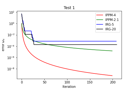
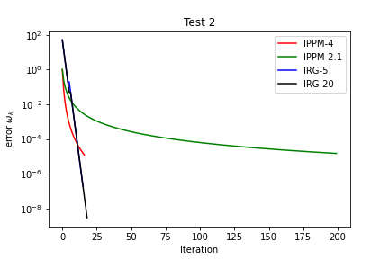
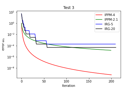
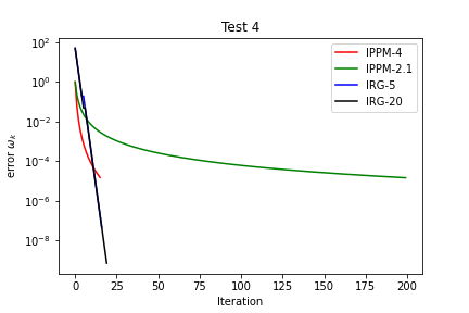
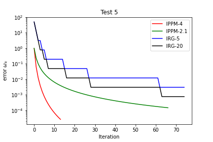
The numerical experiment is conducted on a computer with 10th Gen Intel(R) Core(TM) i5-10400 (6-Core 12M Cache, 2.9GHz to 4.3GHz) and 16GB RAM memory. The codes are written in MATLAB R2021a. The detail information for the results are presented in Table 2, where ’Test #’, ’iter’, ’fval’, ’time’ mean Test number, the number of iterations, value of the objective function at the last iteration and the computational time, respectively. The errors in the inexact proximal point calculations (6.7) and the function values obtained by the algorithms over the duration of time are also graphically illustrated in Figure 4 and Figure 5.
| Test # | m | n | IPPM-2.1 | IPPM-4 | IRG-5 | IRG-20 | ||||||||
|---|---|---|---|---|---|---|---|---|---|---|---|---|---|---|
| iter | fval | time | iter | fval | time | iter | fval | time | iter | fval | time | |||
| 1 | 300 | 300 | 200 | 3.44 | 11.79 | 200 | 3.44 | 100.63 | 209 | 3.44 | 5.51 | 210 | 3.43 | 7.91 |
| 2 | 300 | 600 | 200 | 0.00 | 1.56 | 17 | 0.00 | 0.38 | 16 | 0.00 | 0.33 | 19 | 0.00 | 0.44 |
| 3 | 600 | 600 | 200 | 0.44 | 140.35 | 201 | 0.44 | 863.39 | 210 | 0.44 | 78.09 | 211 | 0.44 | 119.78 |
| 4 | 600 | 1200 | 200 | 0.00 | 5.26 | 16 | 0.00 | 1.72 | 17 | 0.00 | 1.42 | 20 | 0.00 | 1.77 |
| 5 | 1200 | 1200 | 67 | 8.00 | 4000 | 14 | 14.76 | 4000 | 75 | 7.98 | 949.46 | 75 | 8.00 | 1672.52 |


It can be seen from Table 2 that IRG-5 has the best performance in this numerical experiment. IRG-20 is the second fastest algorithm in Tests 1, 3, 5 while it is slightly slower than IPPM-4 in Tests 2, 4. In Test 5 with the largest dimensions IRG-5 is around 4 times faster than IPPM-2.1 while IPPM-4 even cannot reach the value obtained by IPPM-2.1 within the time limit. In this test, IRG-20 is also around 2.5 times faster than IPPM-2.1.
The graphs in Figure 4 and Figure 5 show that the errors (in inexact proximal point calculations) of IRG are automatically adjusted to be suitable for different problems:
- •
In Tests 1, 3, 5 with , it can be seen from Figure 5 that IPPM-2.1 is faster than IPPM-4, which means that the use of larger errors is preferred in this case. Then Figure 4 shows that the errors used in IRG stagnate at most of the iterations. As a result, the IRG methods use the errors larger than that of the IPPM methods and thus achieve better performances.
- •
In Tests 2, 4 with , IPPM-4 with smaller errors performs better than IPPM-2.1. In this cases, the IRG methods decrease in almost every iteration and achieve smaller errors in comparison with IPPM-4.
6.2 Comparison with the exact gradient descent methods
In the numerical experiments presented in this subsection, we show that our IRG method with backtracking stepsize, based on the usage of inexact gradients, performs well compared with the famous methods employing the exact gradient calculation, which are the reduced gradient (RG) method method and gradient descent (GD) method in the following setting:
- 1.
The accuracy of the inexact gradient is low, i.e., , where is not too small relative to .
- 2.
The accuracy required for the solution is increasing.
To demonstrate this, we choose the following two well-known smooth benchmark functions in global optimization taken from the survey paper [28].
- •
The Dixon Price function defined by
The global minimum of this function is , and the two solutions are
and by for all .
- •
The Rosenbrock 1 function defined by
The global minimum of this function is , and the unique solution is .
Since the information about the convexity and the Lipschitz continuity of gradients of the chosen objective functions is unknown, our experiments are conducted by algorithms, where stepsizes are obtained from the corresponding line searches. We use the following abbreviations:
- •
GD: Gradient descent method with the backtracking linesearch.
- •
RGB & IRGB: Reduced gradient method with the backtracking linesearch Inexact reduced gradient method with the backtracking linesearch; see (5.1).
To generate the inexactness for testing purposes, given the gradient error as in (4.10), we create an inexact gradient by adding a random vector with the norm to the exact gradient . To ensure manually controlled errors between the exact gradients and inexact ones that do not decrease so fast, we choose . For all the methods in our experiments, the linesearch parameters are chosen as and . The initial radii and the radius reduction factors are also used for the RG and IRG methods. To avoid the initial points from being identical with the solutions, we choose on tests using the Rosenbrock 1 function. In the tests using the Dixon & Price functions, we choose to avoid the algorithms from going to different solutions. The condition
is used as the stopping criterion for all the tests. The detailed information of the numerical experiments and the achieved numerical results are presented in Table 3. The problem names are given in the forms Dn and Rn, where D stands for Dixon & Price, R stands for Rosenbrock 1, and is the dimension of the tested problem. In these tables, “Iter”, “fval” stand for the number of iterations and the function value at the last iteration.
| Name | GD | IRGB | RGB | |||||||
|---|---|---|---|---|---|---|---|---|---|---|
| Iter | fval | Iter | fval | Iter | fval | |||||
| D200 | 0.01 | 1928 | 2.8E-05 | 1110 | 2.6E-05 | 4.0E-03 | 2.0E-03 | 998 | 2.76E-05 | 4.0E-03 |
| D500 | 0.01 | 3831 | 2.8E-05 | 4782 | 2.7E-05 | 4.0E-03 | 2.0E-03 | 5012 | 2.43E-05 | 4.0E-03 |
| D1000 | 0.01 | 7655 | 2.8E-05 | 9347 | 2.6E-05 | 4.0E-03 | 2.0E-03 | 9271 | 2.58E-05 | 4.0E-03 |
| R200 | 0.01 | 20357 | 9.5E-05 | 24966 | 9.2E-05 | 4.0E-03 | 2.0E-03 | 25162 | 8.65E-05 | 4.0E-03 |
| R500 | 0.01 | 46135 | 9.3E-05 | 59768 | 7.3E-05 | 4.0E-03 | 2.0E-03 | 59604 | 9.20E-05 | 4.0E-03 |
| R1000 | 0.01 | 89130 | 9.4E-05 | 117754 | 8.8E-05 | 4.0E-03 | 2.0E-03 | 117845 | 9.09E-05 | 4.0E-03 |
| D200 | 0.001 | 3294 | 2.7E-07 | 1870 | 2.7E-07 | 4.7E-04 | 2.3E-04 | 1704 | 2.8E-07 | 4.7E-04 |
| D500 | 0.001 | 6543 | 2.8E-07 | 8151 | 2.4E-07 | 4.7E-04 | 2.3E-04 | 7933 | 2.2E-07 | 4.7E-04 |
| D1000 | 0.001 | 13078 | 2.8E-07 | 15946 | 2.7E-07 | 4.7E-04 | 2.3E-04 | 15598 | 2.3E-07 | 4.7E-04 |
| R200 | 0.001 | 22664 | 9.6E-07 | 26958 | 8.9E-07 | 4.7E-04 | 2.3E-04 | 27395 | 9.7E-07 | 4.7E-04 |
| R500 | 0.001 | 48442 | 9.5E-07 | 61998 | 7.8E-07 | 4.7E-04 | 2.3E-04 | 61875 | 9.6E-07 | 4.7E-04 |
| R1000 | 0.001 | 91431 | 9.6E-07 | 119687 | 9.0E-07 | 4.7E-04 | 2.3E-04 | 120321 | 9.6E-07 | 4.7E-04 |
It can be seen that the performance of the IRG and RG methods in Tests D200 with and is better than that of the GD method, while the latter is more efficient in the other tests. It is reasonable that GD usually performs better since it uses the exact gradient while RGB uses the reduced gradient and IRGB uses even the inexact one. In the worst case in Test R1000 with the number of iterations of IRGB is equal around 1.3 times that of GD. It shows that IRGB does not suffer much from the use of inexact gradient compared with the performance of GD using the exact gradient. Table 3 also shows that the decrease of in times results in the increase of the number of iterations in IRGB with the rate at most , where the worst case corresponds with the tests D500. This rate is similar to the rate obtained by the GD method in these tests, which confirms that our IRG method with the backtracking stepsize does not suffer from error accumulation.
The graphs below show that the errors of the inexact gradient used in IRGB is automatically adjusted to be not too small or too large compared with . This confirms the intuitive conclusion on the IRG methods discussed in Remark 4.2(ii). Figure 6 shows that the selections of errors in the existing methods [10, 22, 25] do not fit the unexpected fluctuations in the norm of the exact gradient given in the tests using the Rosenbrock function, which may lead to the over approximation and under approximation issues discussed in Section 1.


7 Conclusions and Further Research
In this paper, we propose and develop the inexact reduced gradient methods with different stepsize selections to solve problems of nonconvex optimization. These methods achieve stationary accumulation points and, under additional assumptions on the KL property of the objective functions, the global linear convergence. The convergence analysis of the developed algorithms is based on novel convergence results established for general linesearch methods. The theoretical and numerical comparisons show that our methods do not suffer much from the error accumulation and are able to automatically adjust the errors in the exact gradient approximations to get a better performance than the existing methods using common selections of errors.
In our future research, we aim at developing the IRG methods in different directions, which include designing zeroth-order algorithms by using practical methods for approximating gradients, designing inexact versions of methods frequently used in nonconvex nonsmooth optimization, e.g., the proximal point and proximal gradient methods, and also designing appropriate IRG methods for problems of constrained optimization. The obtained results would allow us to develop new applications to important classes of models in machine learning, statistics, and related disciplines.
References
- [1] P.-A. Absil, R. Mahony and B. Andrews, Convergence of the iterates of descent methods for analytic cost functions, SIAM J. Optim. 16 (2005), 531–547.
- [2] A. Addis, A. Cassioli, M. Locatelli and F. Schoen, A global optimization method for the design of space trajectories, Comput. Optim. Appl. 48 (2011), 635–652.
- [3] F. J. Aragón Artacho, R. M. T. Fleming and P. T. Vuong, Accelerating the DC algorithm for smooth functions, Math. Program. 169 (2018), 95–118.
- [4] H. Attouch and J. Bolte, On the convergence of the proximal algorithm for nonsmooth functions involving analytic features, Math. Program. 116 (2009), 5–16.
- [5] H. Attouch, J. Bolte, P. Redont and A. Soubeyran, Proximal alternating minimization and projection methods for nonconvex problems. An approach based on the Kurdyka-Łojasiewicz property, Math. Oper. Res. 35 (2010), 438–457.
- [6] H. H. Bauschke, J. Bolte and M. Teboulle, A descent lemma beyond Lipschitz gradient continuity: First-order methods revisited and applications, Math. Oper. Res. 42 (2017), 330–348.
- [7] H. H. Bauschke and P. L. Combettes, Convex Analysis and Monotone Operator Theory in Hilbert Spaces, 2nd edition, Springer. Cham, Switzerland, 2017.
- [8] A. Beck, First-Order Methods in Optimization, SIAM, Philadelphia, PA, 2017.
- [9] A. Beck and M. Teboulle, A fast iterative shrinkage-thresholding algorithm for linear inverse problems, SIAM J. Imaging Sci. 2 (2009), 183–202.
- [10] D. P. Bertsekas, Nonlinear Programming, 3rd edition, Athena Scientific, Belmont, MA, 2016.
- [11] P. Bloomfield and W. Steiger, Least absolute deviations curve fitting, SIAM J. Sci. Stat. Comput. 1 (1980), 290–301.
- [12] J. Bolte, A. Daniilidis and A. Lewis, The Łojasiewicz inequality for nonsmooth subanalytic functions with applications to subgradient dynamical systems, SIAM J. Optim. 17 (2006), 1205–1223.
- [13] J. Bolte, S. Sabach and M. Teboulle, Proximal alternating linearized minimization for nonconvex and nonsmooth problems, Math. Program. 146 (2014), 459–494.
- [14] L. Bottou, F. E. Curtis and J. Nocedal, Optimization methods for large-scale machine learning, SIAM Rev. 60 (2018), 223–311.
- [15] L. M. Bregman, The relaxation method of finding the common point of convex sets and its application to the solution of problems in convex programming, USSR Comput. Math. & Math. Phys. 7 (1967), 200–217.
- [16] J. V. Burke, A. S. Lewis and M. L. Overton, Two numerical methods for optimizing matrix stability, Linear Algebra Appl. 351–352 (2002), 147–184.
- [17] J. V. Burke and Q. Lin, Convergence of the gradient sampling algorithm on directionally Lipschitz functions, Set-Valued Var. Anal. 29 (2021), 949–966.
- [18] F. H. Clarke, Optimization and Nonsmooth Analysis, Wiley, New York, 1983.
- [19] J. B. Crockett and H. Chernoff, Gradient methods of maximization, Pac. J. Math. 5 (1955), 33–50.
- [20] H. B. Curry, The method of steepest descent for non-linear minimization problems, Q. Appl. Math. 2 (1944), 258–261.
- [21] H. Dan, N. Yamashita and M. Fukushima, Convergence properties of the inexact Levenberg-Marquardt method under local error bound conditions, Optim. Meth. Softw. 17 (2002), 605–626
- [22] O. Devolder, F. Glineur and Yu. Nesterov, First-order methods of smooth convex optimization with inexact oracle, Math. Program. 146 (2014), 37–75.
- [23] F. Facchinei, On the convergence to a unique point of minimization algorithms, Technical Report 06-95, Dipartimento di Informacica e Sisemistica, Università di Roma ”La Sapienza”, Rome, Italy, 1995.
- [24] F. Facchinei and J.-S. Pang, Finite-Dimensional Variational Inequalities and Complementarity Problems, Vol. II, Springer, New York, 2003.
- [25] P. Gilmore and C. T. Kelley, An implicit filtering algorithm for optimization of functions with many local minima, SIAM J. Optim. 5 (1995), 269–285.
- [26] A. A. Goldstein, Optimization of Lipschitz continuous functions, Math. Program. 13 (1977), 14–22.
- [27] A. F. Izmailov and M. V. Solodov, Newton-Type Methods for Optimization and Variational Problems, Springer, New York, 2014.
- [28] M. Jamil, A literature survey of benchmark functions for global optimization problems, Int. J. Math. Model. Numer. Optim. 4 (2013), 150–194.
- [29] H. Karimi, J. Nutini and M. Schmidt, Linear convergence of gradient and proximal-gradient methods under the Polyak-Łojasiewicz condition, in Joint European Conference on Machine Learning and Knowledge Discovery in Databases, Lecture Notes in Computer Science, Part 1 (P. Frasconi et al., eds.), Springer, Cham, Switzerland, 2016, pp. 795–811.
- [30] P. D. Khanh, B. S. Mordukhovich, V. T. Phat and D. B. Tran, Generalized damped Newton algorithms in nonsmooth optimization via second-order subdifferentials, J. Global Optim. (2022), https://doi.org/10.1007/s10898-022-01248-7.
- [31] P. D. Khanh, B. S. Mordukhovich, V. T. Phat and D. B. Tran, Globally convergent coderivative-based generalized Newton methods in nonsmooth optimizations, DOI:10.48550/arXiv.2109.02093.
- [32] K. C. Kiwiel, Convergence of the gradient sampling algorithm for nonsmooth nonconvex optimization, SIAM J. Optim. 18 (2007), 379–388.
- [33] K. C. Kiwiel, A nonderivative version of the gradient sampling algorithm for nonsmooth nonconvex optimization, SIAM J. Optim. 20(4), 1983–1994 (2010)
- [34] K. Kurdyka, On gradients of functions definable in o-minimal structures, Ann. Inst. Fourier 48 (1998), 769–783.
- [35] A. S. Lewis, D. R. Luke and J. Malick, Local linear convergence for alternating and averaged nonconvex projections, Found. Comput. Math. 9 (2009), 485-–513.
- [36] H. A. Le Thi, V. N. Huynh and D. T. Pham, Convergence analysis of DC algorithm for DC programming with subanalytic data, J. Optim. Theory Appl. 179 (2018), 103–126.
- [37] S. Łojasiewicz, Ensembles semi-analytiques, Institut des Hautes Etudes Scientifiques, Bures-sur-Yvette (Seine-et-Oise), France, 1965.
- [38] H. Lu, R. M. Freund and Yu. Nesterov, Relatively smooth convex optimization by first-order methods, and applications, SIAM J. Optim. 28 (2018), 333–-354.
- [39] B. S. Mordukhovich, Variational Analysis and Generalized Differentiation, I: Basic Theory, II: Applications, Springer, Berlin, 2006.
- [40] B. S. Mordukhovich, Variational Analysis and Applications, Springer, Cham, Switzerland, 2018.
- [41] Yu. Nesterov, Universal gradient methods for convex optimization problems, Math. Program. 152 (2015), 381–404.
- [42] Yu. Nesterov, Lectures on Convex Optimization, 2nd edition, Springer, Cham, Switzerland, 2018
- [43] M. A. Nielsen, Neural Networks and Deep Learning. Determination Press, New York (2015)
- [44] J. Nocedal and S. J. Wright, Numerical Optimization, 2nd edition. New York, 2016.
- [45] A. Ostrowski, Solution of Equations and Systems of Equations, 2nd edition, Academic Press, New York, 1966.
- [46] B. T. Polyak, Gradient methods for minimizing functionals, USSR Comput. Math. & Math. Phys. 3 (1963), 864–878.
- [47] B. T. Polyak, Introduction to Optimization, Optimization Software, New York, 1987.
- [48] R. T. Rockafellar, Monotone operators and the proximal point algorithm, SIAM J. Control Optim. 14 (1976), 877–898.
- [49] R. T. Rockafellar and R. J-B. Wets, Variational Analysis, Springer, Berlin, 1998.
- [50] T. Rotaru, F. Glineur and P. Patrinos, Tight convergence rates of the gradient method on hypoconvex functions, DOI:10.48550/arXiv.2203.00775
- [51] S. Ruder, An overview of gradient descent optimization algorithms, DOI: 10.48550/arXiv:1609.04747.
- [52] A. Themelis, L. Stella and P. Patrinos, Forward–backward quasi-Newton methods for nonsmooth optimization problems. Comput. Optim. Appl.67 (2017), 443–487.
- [53] Z. Xingyu, On the Fenchel duality between strong convexity and Lipschitz continuous gradient, DOI:10.48550/arXiv.1803.06573.