跳到论文正文
W Papers独立论文阅读器 arXiv:2204.01674 论文正文 计算阅读时间 · 0%
引用这篇论文根据当前论文元数据生成,正式投稿前建议核对。


License: CC BY 4.0
arXiv:2204.01674v2 [math.PR] 15 Jun 2022

Fractal geometry of the space-time difference profile in the directed landscape via construction of geodesic local times

Shirshendu Ganguly Thanks: Department of Statistics, UC Berkeley, Berkeley, CA, USA. e-mail: sganguly@berkeley.edu    Lingfu Zhang Thanks: Department of Mathematics, Princeton University, NJ, USA. e-mail: lingfuz@math.princeton.edu
Abstract

The Directed Landscape, ℒ\mathcal{L}, a random four parameter energy field, was constructed in the breakthrough work of Dauvergne, Ortmann, and Virág [DOV18], and has since been shown in [DV21] to be the scaling limit of various integrable models of Last Passage percolation, a central member of the Kardar-Parisi-Zhang universality class, where one considers the maximum passage time between points attained by weight maximizing paths termed as geodesics. Here ℒ⁡(x,s,y,t)\mathcal{L}(x,s;y,t) denotes the scaled passage time between the points (x,s)(x,s) and (y,t).(y,t). ℒ\mathcal{L} exhibits several scale invariance properties making it a natural source of rich fractal behavior, a topic that has been of constant investigation since its construction. This was initiated in [BGH21], where a novel object called the difference profile: 𝒟⁡(y,t)=ℒ⁡(−1,0,y,t)−ℒ⁡(−1,0,y,t)\mathcal{D}(y,t)=\mathcal{L}(-1,0;y,t)-\mathcal{L}(-1,0;y,t), the difference of passage times from (−1,0)(-1,0) and (1,0)(1,0) to (y,t)(y,t) was introduced. Owing to geodesic geometry, it turns out that this process is almost surely locally constant and the set of non-constancy inherits remarkable fractal properties. In particular, for any fixed t,t, the “spatial process” 𝒟⁡(⋅,t)\mathcal{D}(\cdot,t) is a monotone function, which can be interpreted as the distribution function of a random fractal measure. Across the articles [BGH21, BGH19, GH21, Dau21], it has been established that this random measure is supported on a fractal set of Hausdorff dimension 1/21/2, connected to disjointness of geodesics and bears a rather strong resemblance to Brownian local time. However, the arguments in the above works crucially rely on the aforementioned monotonicity property which is absent when the temporal structure of 𝒟⁡(⋅,⋅)\mathcal{D}(\cdot,\cdot) is probed, necessitating the development of new methods.

In this paper, we put forth several new ideas en-route to computing new fractal exponents governing the same. More precisely, we show that the set of non-constancy of the two dimensional process 𝒟⁡(⋅,⋅)\mathcal{D}(\cdot,\cdot) and the one dimensional temporal process 𝒟⁡(0,⋅)\mathcal{D}(0,\cdot) (a mean zero process owing to symmetry) have Hausdorff dimensions 5/35/3 and 2/32/3 respectively.

Beyond the construction of infinite geodesics, Busemann functions, competition interfaces for ℒ\mathcal{L} (also constructed independently and simultaneously in [RV21] and [BSS22]), all objects of much broader interest, a particularly crucial ingredient in our analysis is the novel construction of a local time process for the geodesic akin to Brownian local time, supported on the “zero set” of the geodesic. Further, we show that the latter has Hausdorff dimension 1/31/3 in contrast to the zero set of Brownian motion which has dimension 1/2.1/2.

Refer to caption
Figure 1: Simulation of the difference profile for the discrete model of Exponential LPP on the positive quadrant ℤ+2\mathbb{Z}^{2}_{+}, rooted at the points (0,50)(0,50) and (50,0)(50,0) and hence defined on the cone emanating from (50,50) (rotated by 45∘45^{\circ}). Colors denote the level sets. (Courtesy of Milind Hegde.)

Contents

1 Introduction

The Kardar-Parisi-Zhang (KPZ) universality class encompasses a broad family of models of one-dimensional random growth which are believed to exhibit certain common features, such as local growth driven by white noise and a smoothing effect from some notion of surface tension and a slope dependent non-linear growth. It is expected that the fluctuation theories of such models are dictated by universal scaling exponents and limiting distributions, exhibited by solutions to a stochastic PDE known as the KPZ equation [Cor12, Cor16, HQ18]. The models known or believed to belong to this collection, include asymmetric exclusion processes, first and last passage percolation, and directed polymers in random media. For these (1+1)(1+1)-dimensional models, the resulting evolution of the growth interface h⁡(t,x)h(t,x) is described by the characteristic triple (1,13,23)(1,\frac{1}{3},\frac{2}{3}) of exponents: at time tt, the value of h⁡(t,x)h(t,x) is of order t1t^{1}, with order t1/3t^{1/3} deviations from its mean, and further, non-trivial correlations are observed when xx is varied on the scale of t2/3t^{2/3}. Furthermore, h⁡(t,x)h(t,x) on proper centering and scaling according to these exponents, is expected to converge to a universal limit t→∞t\to\infty [QR14, MQR16].

Nonetheless, in spite of the breadth of models thought to lie in the class, only a handful have been rigorously shown to do so.An important subclass of models believed to be members of the KPZ universality class is known as last passage percolation (LPP). Ignoring microscopic specifications, in general terms they all consist of an environment of random noise through which directed paths travel, accruing the integral of the noise along it—a quantity known as energy or weight. Given two endpoints, a maximization is done over the weights of all paths with these endpoints with the optimizing path called a geodesic, although, traditionally, the latter is used to denote shortest paths in a metric space.

While most of the above picture is conjectural, recent developments have confirmed the convergence of several exactly solvable models to a well-defined scaling limit. This object was introduced in [DOV18] and named the directed landscape which possesses interesting fractal properties which has been the subject of intense recent study since its construction (see e.g., [Gan21] for an account of such and related advances).

This paper continues this program and makes several novel contributions. Before elaborating on this further, let us introduce the key object of study formally.

1.1 Directed landscape

The directed landscape ℒ\mathcal{L} is a random continuous function from the parameter space

ℝ↑4={u=(p;q)=(x,s,y,t)∈ℝ4:s<t}\mathbb{R}^{4}_{\uparrow}=\{u=(p;q)=(x,s;y,t)\in\mathbb{R}^{4}:s<t\}

to ℝ\mathbb{R} constructed in the breakthrough work [DOV18]. It satisfies the following composition law

ℒ⁡(x,r,z,t)=maxy∈ℝ⁡ℒ⁡(x,r,y,s)+ℒ⁡(y,s,z,t)\mathcal{L}(x,r;z,t)=\max_{y\in\mathbb{R}}\mathcal{L}(x,r;y,s)+\mathcal{L}(y,s;z,t) (1.1)

for any x,z∈ℝx,z\in\mathbb{R} and r<s<tr<s<t. For a continuous path π:[s,t]→ℝ\pi:[s,t]\to\mathbb{R}, its weight under the metric ℒ\mathcal{L} is given by

‖π‖ℒ=infk∈ℕinfs=t0<t1<⋯<tk=t∑i=1kℒ⁡(π⁡(ti−1),ti−1,π⁡(ti),ti).\|\pi\|_{\mathcal{L}}=\inf_{k\in\mathbb{N}}\inf_{s=t_{0}<t_{1}<\cdots<t_{k}=t}\sum_{i=1}^{k}\mathcal{L}(\pi(t_{i-1}),t_{i-1};\pi(t_{i}),t_{i}).

Such a path π\pi is said to be a geodesic from (π⁡(s),s)(\pi(s),s) to (π⁡(t),t)(\pi(t),t) if ‖π‖ℒ=ℒ⁡(π⁡(s),s,π⁡(t),t)\|\pi\|_{\mathcal{L}}=\mathcal{L}(\pi(s),s;\pi(t),t). It is shown in [DOV18] that almost surely, there exists at least one geodesic from pp to qq for any u=(p;q)=(x,s,y,t)∈ℝ↑4u=(p;q)=(x,s;y,t)\in\mathbb{R}^{4}_{\uparrow}. We let πu=π(p;q)=π(x,s,y,t)\pi_{u}=\pi_{(p;q)}=\pi_{(x,s;y,t)} denote any such geodesic from pp to qq. Further, for any fixed u∈ℝ↑4u\in\mathbb{R}^{4}_{\uparrow}, almost surely the geodesic πu\pi_{u} is unique.
Semi-infinite geodesics: Going beyond finite geodesics, for each p=(x,s)∈ℝ2p=(x,s)\in\mathbb{R}^{2} and r∈ℝr\in\mathbb{R}, we denote by πpr:[s,∞)→ℝ\pi_{p}^{r}:[s,\infty)\to\mathbb{R} a semi-infinite geodesic started from pp in the rr direction; i.e. we have t−1​πpr​(t)→rt^{-1}\pi_{p}^{r}(t)\to r as t→∞t\to\infty, and for any s≤s1<s2<∞s\leq s_{1}<s_{2}<\infty, the restriction of πpr\pi_{p}^{r} on [s1,s2][s_{1},s_{2}] is a geodesic (from (πpr​(s1),s1)(\pi_{p}^{r}(s_{1}),s_{1}) to (πpr​(s2),s2)(\pi_{p}^{r}(s_{2}),s_{2})). When r=0r=0, we will drop the rr dependence and simply use πp=πp0\pi_{p}=\pi_{p}^{0}. The issues regarding the existence and uniqueness of such semi-infinite geodesics are not straightforward and will be addressed in Section 4.

The landscape admits invariance under appropriate scalings guided by the exponent triple (1,1/3,2/3)(1,1/3,2/3), much like Brownian motion which is invariant under diffusive scaling. Hence, as in the case of the latter, ℒ\mathcal{L} is expected to exhibit various fractal or self-similar properties.

The present paper continues a recently initiated program devoted to studying such properties and makes several novel contributions.

While the main motivation of the paper lies in studying an object called the “difference profile”, to be defined shortly, en-route we introduce the geodesic local time (GLT), analogous to the classical Brownian local time (BLT), an object we expect to be independently interesting on its own, much akin to its Brownian counterpart which has witnessed intense investigation since its construction by Lévy (see the monograph [BC91] for a beautiful account of the remarkable properties of BLT, and [MP10, Section 6] for a comprehensive treatment).

Thus, one of the main contributions of this paper is to formally construct, for the semi-infinite geodesic π(0,0)\pi_{(0,0)}, its local time, a non-decreasing function L:ℝ≥0→ℝL:\mathbb{R}_{\geq 0}\to\mathbb{R} recording how much time π(0,0)\pi_{(0,0)} has spent at 00. Further, while much remains to be understood about LL, we do succeed in establishing some of its properties, tailored for our applications, such as Hölder regularity and the fractal dimension of its support.

We now move towards defining the aforementioned difference profile, an object introduced in [BGH21] and subsequently the subject of several recent works [BGH19, GH21, Dau21].

To motivate its origin, we begin by pointing out that another central object in the KPZ universality class which had been rigorously established much before ℒ\mathcal{L}, is known as the parabolic Airy2 process, 𝒫1:ℝ→ℝ\mathcal{P}_{1}:\mathbb{R}\to\mathbb{R} [PS02] obtained as the projection ℒ(0,0,⋅,1)\mathcal{L}(0,0,\cdot,1), i.e., when the second spatial coordinate is allowed to vary while the remaining space coordinate is fixed to be 00 and the two temporal coordinates are frozen to be 00 and 11 respectively. In words, the parabolic Airy2 process traces out the last passage time in ℒ\mathcal{L} from the origin to the points (⋅,1).(\cdot,1).

However, by natural translation invariant properties of ℒ,\mathcal{L}, we have the following equality in distribution (among many other symmetries, see e.g., Lemma 3.7) for any y∈ℝ,y\in\mathbb{R},

ℒ(0,0;⋅,1)=𝑑ℒ(y,0;y+⋅,1).\mathcal{L}(0,0;\cdot,1)\overset{d}{=}\mathcal{L}(y,0;y+\cdot,1).

Thus the landscape ℒ\mathcal{L} provides a natural coupling of infinitely many parabolic Airy2 processes “rooted” at different spatial points, making the coupling structure an intriguing object of study. Such a study was initiated in [BGH21], who introduced the following process, which, as we will soon see, encodes valuable information about the coupling.

Difference profile: Fix ya,yb∈ℝy_{a},y_{b}\in\mathbb{R} with ya<yby_{a}<y_{b}. Consider the random function 𝒟:ℍ→ℝ\mathcal{D}:\mathbb{H}\to\mathbb{R} (where ℍ=ℝ×ℝ+\mathbb{H}=\mathbb{R}\times\mathbb{R}_{+} denotes the upper half plane) given by

𝒟⁡(x,t)=ℒ⁡(ya,0,x,t)−ℒ⁡(yb,0,x,t).\mathcal{D}(x,t)=\mathcal{L}(y_{a},0,x,t)-\mathcal{L}(y_{b},0,x,t). (1.2)

We will call 𝒟\mathcal{D} the weight difference profile; it is the difference in the weights of two geodesics with differing but fixed starting points and a common ending point as the latter varies.

For concreteness, we will fix ya=−1y_{a}=-1 and yb=1y_{b}=1 respectively.

Much of this paper is devoted towards computing new fractal exponents associated to 𝒟\mathcal{D}. Since its introduction in [BGH21], several of its properties have already been recorded in the literature. We list some of them below.

Owing to certain key properties of geodesics, it turns out that 𝒟\mathcal{D} is almost everywhere locally constant, with probability one (while this is a consequence of known arguments, this has not been completely spelled out in the literature. One of our main results, Theorem 2.1, will in fact imply this). Further, the following is known.

Lemma 1.1.

Almost surely, for any fixed t,t, 𝒟⁡(⋅,t)\mathcal{D}(\cdot,t) is a continuous non-increasing function.

This has been proved several times in the literature, for example [DOV18, Lemma 9.1] or [BGH21, Theorem 1.1(2)]. Thus, in particular, Lemma 1.1 implies that, for any fixed t,t, at any given point xx, 𝒟⁡(x,t)\mathcal{D}(x,t) is either constant in a neighborhood of xx or decreasing at xx on at least one side.

Moreover, it is an easy argument that the non-constant points of a continuous non-increasing function must form a perfect set, i.e., be closed and have no isolated points. Perfect sets must necessarily be uncountable. In particular, −𝒟⁡(⋅,t)-\mathcal{D}(\cdot,t) can be interpreted as the distribution function of a random measure supported on the uncountable set 𝖭𝖢¯t\overline{\mathsf{NC}}_{t} (the notation 𝖭𝖢¯t\overline{\mathsf{NC}}_{t} is chosen to be in correspondence with the 2D and temporal counterparts 𝖭𝖢\mathsf{NC} and 𝖭𝖢^x\widehat{\mathsf{NC}}_{x}, to be defined shortly). Canonical examples of a similar nature include the Cantor function or the non-constant points of BLT. Associated to any such set is its fractal dimension, which quantifies how “sparse” the set is. With the dimension of the mentioned two examples being classically known, one is led to ask: what is the fractal dimension of 𝖭𝖢¯t\overline{\mathsf{NC}}_{t}?

This question was originally raised and answered in [BGH21], where it was shown that the Hausdorff dimension of 𝖭𝖢¯t\overline{\mathsf{NC}}_{t} is 12\frac{1}{2} almost surely. (The definition of the Hausdorff dimension of a set is recalled ahead in Definition 2.5 for the reader’s convenience.) Further, in [BGH19], it was shown that 𝖭𝖢¯t\overline{\mathsf{NC}}_{t} is precisely the set of points x,x, which admit geodesics to the points (−1,0)(-1,0) and (1,0)(1,0) respectively, which are disjoint except at their initial point (x,t).(x,t). Finally, more recently, in [GH21] (and subsequently [Dau21]), comparisons were made between 𝒟⁡(⋅,t)\mathcal{D}(\cdot,t) and BLT, showing, among other things, that the former is absolutely continuous with respect to the latter in a certain precise sense.

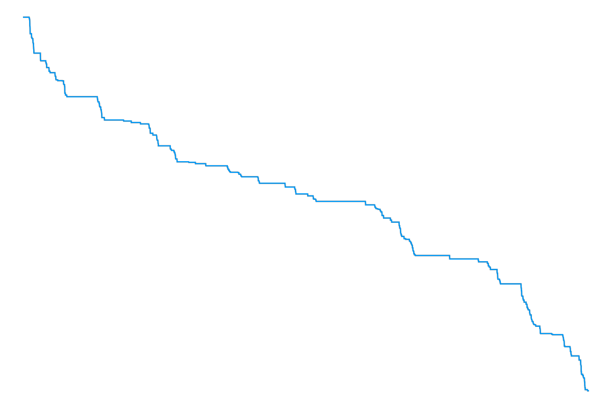
However, in all the above works, the monotonicity of 𝒟⁡(⋅,t)\mathcal{D}(\cdot,t) was crucially used with the arguments breaking down if the temporal coordinate was varied instead, in which case the process 𝒟⁡(x,⋅)\mathcal{D}(x,\cdot) is no longer monotone, necessitating the development of new ideas. (See Figure 2 for simulations of 𝒟\mathcal{D}.)

This is the main purpose of this article. Thus, to summarize, we will investigate the spatio-temporal behavior of the process 𝒟\mathcal{D} and compute new fractal dimensions associated to it. As a key ingredient, we introduce and study the notion of GLT, an object we anticipate to be of broader interest and applicability. The connection between the difference profile and GLT is established through a novel level set decomposition which is presented shortly, in Section 2.3.
Refer to caption
Refer to caption
Figure 2: Simulations of the difference profile 𝒟\mathcal{D}: the left panel is 𝒟⁡(⋅,1)\mathcal{D}(\cdot,1), and the right panel is 𝒟⁡(0,⋅)\mathcal{D}(0,\cdot). (Courtesy of Milind Hegde.)

We now proceed to stating our main results.

2 Main results

As indicated already, the key object of our investigation is the difference profile 𝒟⁡(x,t)=ℒ⁡(−1,0,x,t)−ℒ⁡(1,0,x,t).\mathcal{D}(x,t)=\mathcal{L}(-1,0;x,t)-\mathcal{L}(1,0;x,t).

2.1 Fractal properties of the difference profile

Our main results pertain to the fractal dimension of the support set of 𝒟\mathcal{D} which is almost surely locally constant. To this end, we define 𝖭𝖢⊂ℍ\mathsf{NC}\subset\mathbb{H} to be the set of all (x,t)(x,t) where the difference profile 𝒟\mathcal{D} is not constant in a neighborhood. A one dimensional variant is 𝖭𝖢^x⊂ℝ+\widehat{\mathsf{NC}}_{x}\subset\mathbb{R}_{+} consisting of all tt such that the function t↦𝒟⁡(x,t)t\mapsto\mathcal{D}(x,t) is not constant in a neighborhood of tt. We note that 𝖭𝖢^x⊂{t∈ℝ+:(x,t)∈𝖭𝖢}\widehat{\mathsf{NC}}_{x}\subset\{t\in\mathbb{R}_{+}:(x,t)\in\mathsf{NC}\}. The set 𝖭𝖢^x\widehat{\mathsf{NC}}_{x} is exactly the temporal analogue of the spatial set 𝖭𝖢¯t\overline{\mathsf{NC}}_{t} of all xx such that 𝒟⁡(x,t)\mathcal{D}(x,t) is not locally constant, considered in the papers [BGH21, BGH19, GH21, Dau21]. As we will mostly work with the temporal non-constant set at x=0x=0, we let 𝖭𝖢^=𝖭𝖢^0\widehat{\mathsf{NC}}=\widehat{\mathsf{NC}}_{0}.

With the above preparation, we can now state our two main results.

Theorem 2.1.

Almost surely, the set 𝖭𝖢\mathsf{NC} has Hausdorff dimension 5/35/3.

Theorem 2.2.

Almost surely, the set 𝖭𝖢^\widehat{\mathsf{NC}} has Hausdorff dimension 2/32/3.

As the reader will notice from the arguments presented in the paper, unlike the process 𝒟⁡(⋅,t)\mathcal{D}(\cdot,t) which is monotone and decreases from −∞-\infty to ∞\infty as xx varies on ℝ,\mathbb{R}, the temporal process 𝒟⁡(0,⋅)\mathcal{D}(0,\cdot) eventually becomes a constant owing to geodesic coalescence. Further, the process, almost surely, changes sign infinitely often as tt approaches 00 owing to symmetry, de-correlation across different values of tt as the latter converges to 00 suitably fast, and ergodicity of the directed landscape.

As already indicated in the introduction, the proofs of our main theorems rely on a key ingredient, namely, a novel construction of the geodesic local time (GLT), and analysis of its fractal properties which we include as our final main result. Recall that we use πpr\pi_{p}^{r} to denote the semi-infinite geodesic started from pp in the rr direction (the formal treatement will appear in Section 4), and write πp=πp0\pi_{p}=\pi_{p}^{0}.

2.2 The geodesic local time

Throughout this paper we let 𝟎\mathbf{0} denote the origin (0,0)(0,0). Consider the geodesic π𝟎\pi_{\mathbf{0}}, and its intersection with the line {(0,t):t≥0}\{(0,t):t\geq 0\}. Denote by

Z:={t≥0:π𝟎​(t)=0},Z:=\{t\geq 0:\pi_{\mathbf{0}}(t)=0\}, (2.1)

the geodesic zero set.

Theorem 2.3.

Almost surely, the set ZZ has Hausdorff dimension 1/31/3.

The proofs of all these three theorems rely on the construction of GLT, a non-decreasing function L:ℝ≥0→ℝL:\mathbb{R}_{\geq 0}\to\mathbb{R}, which records the time π𝟎\pi_{\mathbf{0}} has spent at 00. This induces a (random) measure μ\mu on ℝ≥0\mathbb{R}_{\geq 0}, supported on the set ZZ similar to how BLT is supported on the zero set of Brownian motion. An important step in the construction of LL is the construction of the geodesic occupation measure. We define the occupation measure νh\nu_{h} for the geodesic π𝟎\pi_{\mathbf{0}} at height hh, by setting for any measurable A⊂ℝA\subset\mathbb{R},

νh(A)=∫0h𝟙[π𝟎(t)∈A]dt.\nu_{h}(A)=\int_{0}^{h}\mathds{1}[\pi_{\mathbf{0}}(t)\in A]dt. (2.2)

Given the above, the construction of LL is completed by proving the existence of the density of νh\nu_{h} at 00.

Proposition 2.4.

For any height h>0,h>0, almost surely the limit limw↘0(2​w)−1​νh​([−w,w])\lim_{w\searrow 0}(2w)^{-1}\nu_{h}([-w,w]) exists and is finite.

Before proceeding further, it is worth pointing out some other recent advances around the theme of fractal properties of last passage percolation. While the works [JRA20, JRAS19, SS21a] focussed on pre-limiting models, [CHHM21, Dau22] worked with the evolution induced by the directed landscape started from rather general initial data (an object termed as the KPZ-fixed point, see [MQR16]). In another direction, fractal properties often manifests in remarkable behavior of the system pertaining to “chaos and noise-sensitivity”. Refer e.g. to the success story of the study of dynamical critical percolation summarized beautifully in [GS14]. In the KPZ universality paradigm, such a study was initiated recently in [GH20b].

2.3 Key ideas in the proofs

The arguments in this paper involve several new ideas, which we describe in some detail in this section.

We first setup some notations that will be used throughout this paper. For any set A,A, we use |A||A| to denote its cardinality. We use ℒ\mathscr{L} to denote the Lebesgue measure on ℝ\mathbb{R}. The notation ∥⋅∥\|\cdot\| denotes the l2l^{2} norm unless otherwise stated. Recall that we let 𝟎=(0,0)\mathbf{0}=(0,0). For any a≤ba\leq b, we let ⟦a,b⟧=[a,b]∩ℤ\llbracket a,b\rrbracket=[a,b]\cap\mathbb{Z}. We would need to consider the space of all non-empty compact subsets of ℝ2\mathbb{R}^{2} which equipped with the Hausdorff metric, becomes a complete metric space, with the induced topology referred to as the Hausdorff topology. We will also freely use the notation argmax\argmax even when there isn’t a unique maximum (but there must exist at least one) using it to denote an arbitrary one.

We next recall the definitions of the Hausdorff dimension and Hausdorff measure of a set.

Definition 2.5.

For any d≥0d\geq 0 and metric space XX, the dd-dimensional Hausdorff measure of XX is defined as

limδ↘0inf{∑idiam⁡(Ui)d:{Ui}​ is a countable cover of ​X​ with ​0<diam⁡(Ui)<δ}.\lim_{\delta\searrow 0}\inf\left\{\sum_{i}\diam(U_{i})^{d}:\{U_{i}\}\text{ is a countable cover of }X\text{ with }0<\diam(U_{i})<\delta\right\}.

The Hausdorff dimension of XX is inf{d>0: the d-dimensional Hausdorff measure of X is zero }\inf\{d>0:\text{ the $d$-dimensional Hausdorff measure of $X$ is zero }\}.

We start by stating two general strategies to obtain upper and lower bounds for the Hausdorff dimension for XX being a subset of ℝn\mathbb{R}^{n} (for some n∈ℕn\in\mathbb{N}).

  • •

    Upper bound: Show that for any U⊂ℝnU\subset\mathbb{R}^{n}, ℙ[X∩U≠∅]<diam(U)n−d\mathbb{P}[X\cap U\neq\emptyset]<\diam(U)^{n-d} (potentially with some extra logarithmic factors). Then for any compact S⊂ℝnS\subset\mathbb{R}^{n}, on dividing SS into roughly δ−n\delta^{-n} subsets, each with diameter ≤δ\leq\delta, XX is covered by the union of roughly δ−d\delta^{-d} of them. Thus for any ϵ>0\epsilon>0, the d+ϵd+\epsilon-dimensional Hausdorff measure of XX is zero. So the Hausdorff dimension of XX is at most dd.

  • •

    Lower bound: This is usually the harder direction and involves constructing a measure mm whose support is contained in XX, such that m⁡(X)>0m(X)>0, and for any measurable U⊂XU\subset X the Hölder estimate m⁡(U)<diam⁡(U)dm(U)<\diam(U)^{d} (potentially with extra sub-polynomial factors) holds. Then for any countable cover {Ui}\{U_{i}\} of XX, one must have ∑idiam⁡(Ui)d>m⁡(X)\sum_{i}\diam(U_{i})^{d}>m(X), implying that the Hausdorff dimension of XX is at least dd.

Before diving into our arguments, for contrast, let us first briefly sketch the nature of the arguments appearing in the analysis of 𝒟⁡(⋅,t)\mathcal{D}(\cdot,t) in [BGH21] (from here on we will fix t=1t=1) and why they fail in the case of 𝒟⁡(x,⋅)\mathcal{D}(x,\cdot) (we will fix x=0x=0). A key starting observation in [BGH21] is the following (also see Figure 3(a)): for two points x1<x2,x_{1}<x_{2}, 𝒟⁡(x,1)\mathcal{D}(x,1) is constant on [x1,x2][x_{1},x_{2}] if the geodesics π(−1,0,x1,1)\pi_{(-1,0;x_{1},1)} π(1,0,x2,1)\pi_{(1,0;x_{2},1)} coalesce.

(−1,0)(-1,0)(1,0)(1,0)(x1,1)(x_{1},1)(x2,1)(x_{2},1)
(a) If the geodesics π(−1,0,x1,1)\pi_{(-1,0;x_{1},1)} and π(1,0,x2,1)\pi_{(1,0;x_{2},1)} coalesce, any geodesic from (−1,0)(-1,0) or (1,0)(1,0) to any (x,1)(x,1) with x∈[x1,x2]x\in[x_{1},x_{2}] must stay with π(−1,0,x1,1)\pi_{(-1,0;x_{1},1)} or π(1,0,x2,1)\pi_{(1,0;x_{2},1)} up to the end of their intersection. This implies that 𝒟⁡(x,1)\mathcal{D}(x,1) is constant on [x1,x2][x_{1},x_{2}].
(−1,0)(-1,0)(1,0)(1,0)(0,t1)(0,t_{1})(z,t1)(z,t_{1})(0,t2)(0,t_{2})
(b) If all geodesics from (−1,0)(-1,0) and (1,0)(1,0) to (x,t1)(x,t_{1}) coalescence, for xx in an order (t2−t1)2/3(t_{2}-t_{1})^{2/3} neighborhood of 00, the process 𝒟⁡(0,⋅)\mathcal{D}(0,\cdot) is (likely to be) constant on [t1,t2][t_{1},t_{2}].
Figure 3: Illustrations for the arguments in [BGH21] (for upper bounding the Hausdorff dimension), and the same strategy in the temporal direction.

Thus to prove an upper bound on the Hausdorff dimension of 𝖭𝖢¯1,\overline{\mathsf{NC}}_{1}, [BGH21] uses as input the following estimate from [Ham20]: For any x1<x2x_{1}<x_{2}, y1<y2y_{1}<y_{2}, and s<ts<t, if we let Disj(x1,x2)→(y1,y2)[s,t]\Dist_{(x_{1},x_{2})\to(y_{1},y_{2})}^{[s,t]} be the event that π(x1,s,y1,t)\pi_{(x_{1},s;y_{1},t)} and π(x2,s,y2,t)\pi_{(x_{2},s;y_{2},t)} are unique and disjoint, then

Theorem 2.6.

There is a constant CC, such that for any ϵ>0\epsilon>0, we have

ℙ⁡[Disj(−1,1)→(−ϵ,ϵ)[0,1]]<C​ϵ1/2​eC​|log⁡(ϵ)|5/6.\mathbb{P}[\Dist_{(-1,1)\to(-\epsilon,\epsilon)}^{[0,1]}]<C\epsilon^{1/2}e^{C|\log(\epsilon)|^{5/6}}.

Thus, for any small ϵ,\epsilon, ignoring sub-polynomial factors, the probability that 𝖭𝖢¯1\overline{\mathsf{NC}}_{1} intersects any interval of size ϵ\epsilon is at most ϵ1/2\epsilon^{1/2}, which then leads to an upper bound of 1/21/2 on the Hausdorff dimension, according to the above general strategy.

For the lower bound, the argument relies on Hölder regularity of ℒ.\mathcal{L}. Namely that the Parabolic Airy2 process is locally 1/2−1/2- Hölder-regular (in fact it is globally parabolic and locally Brownian, see e.g., [CH14, Ham16, CHH19]) and so is 𝒟⁡(⋅,1)\mathcal{D}(\cdot,1) being the difference of two Airy2 processes rooted at ±1\pm 1. By interpreting −𝒟⁡(⋅,1)-\mathcal{D}(\cdot,1) as the distribution function of a measure and the above general strategy, we get a Hausdorff dimension lower bound of 1/21/2.

It is instructive to apply now the same strategy to analyze the process 𝒟⁡(0,⋅)\mathcal{D}(0,\cdot) instead (also see Figure 3(b)). For two points t1<t2t_{1}<t_{2}, consider the geodesics π(−1,0,0,t1)\pi_{(-1,0;0,t_{1})} and π(1,0,0,t2).\pi_{(1,0;0,t_{2})}. Let the latter intersect the line t=t1t=t_{1} at location z,z, then by a similar argument as before, one can essentially conclude (the precise conclusion is somewhat different which we will not spell out here) that 𝒟⁡(0,⋅)\mathcal{D}(0,\cdot) is constant on [t1,t2][t_{1},t_{2}] unless the geodesics π(−1,0,0,t1)\pi_{(-1,0;0,t_{1})} and π(1,0,z,t1)\pi_{(1,0;z,t_{1})} are disjoint. Now, it is known, and goes back to the work of Johansson [Joh00] (see also [BSS14, HS20, DSV20]), that the geodesics in LPP and hence ℒ\mathcal{L} are 2/3−2/3- Hölder-regular, which then implies that z≈|t2−t1|2/3.z\approx|t_{2}-t_{1}|^{2/3}. This in conjunction with the above estimate on existence of disjoint geodesics imply that the probability that 𝖭𝖢^\widehat{\mathsf{NC}} intersects [t1,t2][t_{1},t_{2}] is at most, up to sub-polynomial factors, |t2−t1|1/3|t_{2}-t_{1}|^{1/3} which translates into a Hausdorff dimension upper bound of 2/32/3 for 𝖭𝖢^.\widehat{\mathsf{NC}}.

On the other hand, applying the same reasoning as before, we now seek to use the fact that ℒ\mathcal{L} is 1/3−1/3- Hölder-regular in the temporal direction, implying at least as much regularity for 𝒟⁡(0,⋅)\mathcal{D}(0,\cdot). This then yields, again by the above general strategy, a lower bound of 1/31/3 for the Hausdorff dimension which unlike the spatial case, falls short of matching the upper bound.

The reason for the disparity is that the process 𝒟⁡(0,⋅)\mathcal{D}(0,\cdot) is a mean zero process and hence not monotone. In the spatial case, when applying the above general strategy, the process 𝒟⁡(⋅,1)\mathcal{D}(\cdot,1) was itself inducing a measure owing to monotonicity, whereas the process 𝒟⁡(0,⋅)\mathcal{D}(0,\cdot) induces a signed measure instead. Thus the argument which essentially works with the “absolute value” of the measure, or the “un-signed” measure fails to capture certain cancellations exhibited by 𝒟⁡(0,⋅),\mathcal{D}(0,\cdot), which we expect leads to a square-root fluctuation effect boosting the lower bound from 1/31/3 to 2/3.2/3.

Thus to obtain a sharp lower bound we will seek to construct new measures capturing the appropriate cancellation. This involves many new ideas and is quite technical. We will review the key steps in the sequel but first let us digress a bit allowing us to introduce a few new objects which will play central roles in our arguments.

GLT and the zero set: As is the case in Brownian motion, the zero set of the semi-infinite geodesic π𝟎\pi_{\mathbf{0}} (see the beginning of Section 2.2) denoted by ZZ, will turn out to be a particularly fundamental object. As indicated in Section 2.2, we will construct GLT LL and show that it is 1/31/3 Hölder-regular, and using that we will show that ZZ has Hausdorff dimension 1/31/3 (as stated in Theorem 2.3). This will follow from the following estimate, whose proof will be briefly reviewed at the end of this section:

Lemma 2.7.

There are universal constants C,c>0C,c>0 such that the following is true. For any closed interval I⊂ℝI\subset\mathbb{R} and J⊂ℝ≥0J\subset\mathbb{R}_{\geq 0}, we have

ℙ[ℒ({t∈J:π𝟎(t)∈I})>Mℒ(I)ℒ(J)1/3]<Ce−c​M\mathbb{P}[\mathscr{L}(\{t\in J:\pi_{\mathbf{0}}(t)\in I\})>M\mathscr{L}(I)\mathscr{L}(J)^{1/3}]<Ce^{-cM}

for any M>0M>0.

Competition interfaces: The next object that we need to consider pertains to level sets. As is perhaps not surprising from the fact that we are investigating the behavior of the difference profile 𝒟\mathcal{D}, it would be particularly convenient to consider level sets of the form

ϑℓ​(t)=inf{x∈ℝ:𝒟⁡(x,t)≤ℓ}.\vartheta_{\ell}(t)=\inf\{x\in\mathbb{R}:\mathcal{D}(x,t)\leq\ell\}. (2.3)

It turns out however that a remarkable identity holds if we were to take ℓ=0\ell=0 and consider the difference profile not rooted at ±1\pm 1, but with Brownian initial data instead. Namely, let ℬ\mathcal{B} be a standard two sided Brownian motion. For any x∈ℝ,t>0x\in\mathbb{R},t>0, we let

ℒL​(x,t)\displaystyle\mathcal{L}^{L}(x,t) =supy≤0ℒ⁡(y,0,x,t)+ℬ⁡(y),\displaystyle=\sup_{y\leq 0}\mathcal{L}(y,0;x,t)+\mathcal{B}(y),
ℒR​(x,t)\displaystyle\mathcal{L}^{R}(x,t) =supy≥0ℒ⁡(y,0,x,t)+ℬ⁡(y),\displaystyle=\sup_{y\geq 0}\mathcal{L}(y,0;x,t)+\mathcal{B}(y),

be the passage times induced by the Brownian initial data from the negative and positive parts of the x−x-axis respectively. One can show that the function x↦ℒL​(x,t)−ℒR​(x,t)x\mapsto\mathcal{L}^{L}(x,t)-\mathcal{L}^{R}(x,t) is non-increasing in xx (see the beginning of Section 5). We then let

ϑℬ​(t)=inf{x∈ℝ:ℒL​(x,t)−ℒR​(x,t)≤0}.\vartheta^{\mathcal{B}}(t)=\inf\{x\in\mathbb{R}:\mathcal{L}^{L}(x,t)-\mathcal{L}^{R}(x,t)\leq 0\}. (2.4)

One then has the remarkable duality result:

Proposition 2.8.

The processes ϑℬ\vartheta^{\mathcal{B}} and π𝟎\pi_{\mathbf{0}} are equal in distribution.

In the discrete setting (of exponential LPP), this goes back to [FP05, BCS06, FMP09], and we get the above directed landscape version using a limit transition from [DV21]. During the preparation of this paper, two articles [RV21, SS21b] were posted on the arXiv where this was independently developed. While [RV21] worked with the directed landscape as in the present paper, [SS21b] considered the prelimiting model of Brownian LPP instead.

Now, how does this help us? Suppose for the moment that the same were true for the level sets ϑℓ​(⋅)\vartheta_{\ell}(\cdot) for all ℓ\ell, in place of ϑℬ​(⋅).\vartheta^{\mathcal{B}}(\cdot). Recalling that we only seek to prove a lower bound of 2/32/3 for the Hausdorff dimension of 𝖭𝖢^,\widehat{\mathsf{NC}}, we will now construct a measure supported on 𝖭𝖢^\widehat{\mathsf{NC}} which will be 2/32/3 Hölder-regular. At a very high level, this is achieved by taking the average of the local time for each of the level sets. The construction proceeds as in the case of GLT. Now using the above assumed comparison between level sets and the geodesic, it follows that each of the individual level set local times are 1/31/3 Hölder-regular using Lemma 2.7. Given this, we obtain the desired 2/32/3 Hölder regularity, using Hölder regularity of ℒ\mathcal{L}.

To see this, consider an interval [t1,t2].[t_{1},t_{2}]. Now each ϑℓ\vartheta_{\ell} induces a 1/31/3 Hölder-regular measure κℓ\kappa_{\ell}. To define this we start by defining the corresponding occupation measures analogous to (2.2). For each h>0h>0, we denote by λℓ,h\lambda_{\ell,h} the measure on ℝ\mathbb{R}, such that

λℓ,h(A)=∫0h𝟙[ϑℓ(t)∈A]dt,\lambda_{\ell,h}(A)=\int_{0}^{h}\mathds{1}[\vartheta_{\ell}(t)\in A]dt, (2.5)

for any measurable A⊂ℝA\subset\mathbb{R}. Given this, κℓ\kappa_{\ell} on an interval (g,h)(g,h) is then defined to be the density of λℓ,h−λℓ,g\lambda_{\ell,h}-\lambda_{\ell,g} at 0,0, that is,

κℓ​((g,h))=limw↘0(2​w)−1​(λℓ,h​([−w,w])−λℓ,g​([−w,w])).\kappa_{\ell}((g,h))=\lim_{w\searrow 0}(2w)^{-1}(\lambda_{\ell,h}([-w,w])-\lambda_{\ell,g}([-w,w])). (2.6)

(The actual definition proceeds a bit differently owing to certain measure theoretic considerations which we will ignore in this discussion). Define now the measure κ\kappa by setting

κ⁡(A)=∫κℓ​(A)​𝑑ℓ.\kappa(A)=\int\kappa_{\ell}(A)d\ell. (2.7)
(0,0)(0,0)(0,t1)(0,t_{1})(0,t2)(0,t_{2})ϑℓ1\vartheta_{\ell_{1}}ϑℓ2\vartheta_{\ell_{2}}
(a) If both ϑℓ1\vartheta_{\ell_{1}} and ϑℓ2\vartheta_{\ell_{2}} intersect the interval {0}×[t1,t2]\{0\}\times[t_{1},t_{2}], it is likely that |ℓ2−ℓ1||\ell_{2}-\ell_{1}| is in the order of at most |t2−t1|1/3|t_{2}-t_{1}|^{1/3}.
𝟎\mathbf{0}ℬ\mathcal{B}
(b) An illustration of the event where the Brownian motion ℬ\mathcal{B} has a very spiky behavior with spikes near ±1\pm 1, and geodesic coalescence.
Figure 4:

This is the measure that we use to lower bound the Hausdorff dimension of 𝖭𝖢^\widehat{\mathsf{NC}} by showing that κ\kappa is supported in 𝖭𝖢^\widehat{\mathsf{NC}} and further for any interval [t1,t2],[t_{1},t_{2}], κ⁡([t1,t2])≈|t2−t1|2/3.\kappa([t_{1},t_{2}])\approx|t_{2}-t_{1}|^{2/3}. Very briefly, the latter holds because by definition κ⁡([t1,t2])=∫κℓ​([t1,t2])​𝑑ℓ.\kappa([t_{1},t_{2}])=\int\kappa_{\ell}([t_{1},t_{2}])d\ell. Now by the claimed 1/31/3 Hölder regularity of GLT and the assumed comparison between κℓ\kappa_{\ell} and the same, the integrand is at most |t2−t1|1/3.|t_{2}-t_{1}|^{1/3}. Now by the 1/31/3 Hölder regularity of the landscape in the temporal direction (a consequence of 1/31/3 being the universal exponent governing weight fluctuations in the KPZ universality class), for ϑℓ1\vartheta_{\ell_{1}} and ϑℓ2\vartheta_{\ell_{2}} to both intersect the interval {0}×[t1,t2]\{0\}\times[t_{1},t_{2}], we must have, again ignoring sub-polynomial factors, |ℓ2−ℓ1|≤|t2−t1|1/3|\ell_{2}-\ell_{1}|\leq|t_{2}-t_{1}|^{1/3} (see Figure 4(a)), which yields the desired estimate κ⁡([t1,t2])=∫κℓ​([t1,t2])=O⁡(|t2−t1|2/3)\kappa([t_{1},t_{2}])=\int\kappa_{\ell}([t_{1},t_{2}])=O(|t_{2}-t_{1}|^{2/3}) since the integrand is non-zero only on a interval of size at most |t2−t1|1/3.|t_{2}-t_{1}|^{1/3}.

Note that the above reasoning is contingent on the assumption that the measures κℓ\kappa_{\ell} are 1/31/3 Hölder-regular which was a consequence of the claim that the level curves ϑℓ\vartheta_{\ell} are “similar” to the geodesic π𝟎.\pi_{\mathbf{0}}. We rely on Proposition 2.8 to prove a result of this kind which suffices for our purpose. At a very high level, the arguments in this part is based on the observation that if the Brownian motion ℬ\mathcal{B} has a very spiky behavior with spikes near ±1\pm 1 respectively as in Figure 4(b) then this resembles the original situation of considering the difference profile rooted at ±1\pm 1 respectively. In particular, in presence of such spikes, owing to geodesic coalescence, ϑℬ\vartheta^{\mathcal{B}} is the same as ϑℓ\vartheta_{\ell} for some random ℓ\ell, where the law of the latter dominates a multiple of Lebesgue measure owing to the fluctuation of the difference in the height of the spikes at ±1\pm 1, which can be obtained by resampling suitable parts of ℬ\mathcal{B}.

Theorem 2.1 is proved in the same way as Theorem 2.2 and is in fact somewhat easier technically since instead of working with the “density” measures in (2.6), we work with the occupation measures in (2.5) instead and the “occupation” counterpart of κ\kappa by taking their integral over different values of ℓ\ell. The same set of arguments then concludes the proof. In this case the measure we work with is simply ζ\zeta, such that for any a<ba<b and 0≤g<h0\leq g<h, we let

ζ⁡([a,b]×(g,h))=∫gh[𝒟⁡(a,t)−𝒟⁡(b,t)]​𝑑t=∫ℓ[λℓ,h​([a,b])−λℓ,g​([a,b])]​𝑑ℓ.\zeta([a,b]\times(g,h))=\int_{g}^{h}[\mathcal{D}(a,t)-\mathcal{D}(b,t)]dt=\int_{\ell}[\lambda_{\ell,h}([a,b])-\lambda_{\ell,g}([a,b])]d\ell. (2.8)

Now when b−a=h−g≈ϵ,b-a=h-g\approx\epsilon, using the same argument as before one can conclude that ζ⁡([a,b]×(g,h))≈ϵ5/3\zeta([a,b]\times(g,h))\approx\epsilon^{5/3} leading to the desired lower bound on the dimension.

We end the above discussion by pointing out that while the difference profile 𝒟\mathcal{D} we consider is rooted at (±1,0),(\pm 1,0), one may generalize our argument to a rather general class of “rooting functions” where for functions f1,f2,f_{1},f_{2}, one considers

(x,t)↦supy[ℒ⁡(y,0,x,t)+f1​(y)]−supy[ℒ⁡(y,0,x,t)+f2​(y)].(x,t)\mapsto\sup_{y}[\mathcal{L}(y,0;x,t)+f_{1}(y)]-\sup_{y}[\mathcal{L}(y,0;x,t)+f_{2}(y)].

In particular, for the special case f1,f2:ℝ→ℝ∪{−∞}f_{1},f_{2}:\mathbb{R}\to\mathbb{R}\cup\{-\infty\}, such that (1) they are bounded from above on any compact interval, (2) there exists some x∗>0x_{*}>0 such that f1​(x)=−∞f_{1}(x)=-\infty for any x>−x∗x>-x_{*} and f2​(x)=−∞f_{2}(x)=-\infty for any x<x∗x<x_{*}, (3) lim sup|x|→∞f1​(x)/x2,f2​(x)/x2≤0\limsup_{|x|\to\infty}f_{1}(x)/x^{2},f_{2}(x)/x^{2}\leq 0, essentially our arguments can be carried out without any significant changes to prove the counterparts of Theorems 2.1 and 2.2 in this setting. However we do not pursue spelling out all the details which will be done in future work where more general f1f_{1} and f2f_{2} will be treated as well.

The remainder of the discussion is devoted to providing a brief overview of the ideas going into the other novel aspects of the paper. This includes the construction of the semi-infinite geodesic π𝟎\pi_{\mathbf{0}} as well as the proof of the duality relation with the competition interface (2.4), and finally the construction of GLT and the local times for the level curves (2.3). As already mentioned, these objects and similar ideas have recently appeared on the arXiv in the articles [RV21, SS21b, BSS22] during the preparation of this paper.

Construction of π𝟎\pi_{\mathbf{0}}: The construction relies on geodesic coalescence. To construct a semi-infinite geodesic we show that the finite geodesics π(p,zn,hn),\pi_{(p;z_{n},h_{n})}, for any sequences {zn}n=1∞\{z_{n}\}_{n=1}^{\infty} and {hn}n=1∞\{h_{n}\}_{n=1}^{\infty} satisfying that zn→∞z_{n}\to\infty as n→∞n\to\infty and |zn−hn​r|<hn2/3|z_{n}-h_{n}r|<h_{n}^{2/3} for each n∈ℕn\in\mathbb{N}, owing to geodesic coalescence, all share the same initial segment. Further, the length of the initial segment itself goes off to infinity as n→∞.n\to\infty. π𝟎\pi_{\mathbf{0}} is then defined to be the path made up of such initial segments.

While the construction is intuitive, it does involve some amount of work to show that it works. Namely it has the desired direction. We further show that there is a unique such semi-infinite geodesic.

We will not comment much on how the above is carried out except that we rely on a construction of the Busemann function in the vertical direction (again relying on geodesic coalescence). Busemann functions were originally used to study the large-scale geometry of geodesics in Riemannian manifolds, and was introduced to study general first passage percolation (FPP) models by Hoffman [Hof05, Hof08]. It has also been intensively studied and used in the exponential LPP setting; see e.g. [Sep17]. We then show that in our setting the Busemann function is a Brownian motion and that π𝟎​(t)\pi_{\mathbf{0}}(t), is the argmax of the sum of the Busemann function and an independent copy of an appropriately scale Parabolic Airy2 process. By the known Brownianity of both the functions and their independence, it follows that π𝟎​(t)\pi_{\mathbf{0}}(t) is unique, at least for rational tt and hence for all tt by continuity. Further, it follows by estimates of Brownian motion as well as the Parabolic Airy2 process, that π𝟎​(t)≈O⁡(t2/3)\pi_{\mathbf{0}}(t)\approx O(t^{2/3}) and thereby implying that π𝟎\pi_{\mathbf{0}} indeed has the desired direction.

Proof of duality: The duality is known to hold in the discrete model of Exponential LPP. To prove the directed landscape version, we rely on the recent convergence results proved in [DV21], which in particular implies that both the semi-infinite geodesic and the competition interfaces in the discrete setting converge to their counterparts π𝟎\pi_{\mathbf{0}} and ϑℬ\vartheta^{\mathcal{B}} which is enough to conclude the proof. To be completely precise, however, the results in [DV21] only can be used to deduce convergence of certain “compactified” versions of the above objects. To make use of this, we work with certain truncations of π𝟎\pi_{\mathbf{0}} and ϑℬ\vartheta^{\mathcal{B}}, and their discrete versions, show that with high probability the truncated versions agree with the untruncated ones, the discrete ones converge to the continuous counterparts and hence the discrete duality transfers to the desired continuous duality statement.

Construction of GLT: Akin to the construction of BLT, this proceeds by first constructing the occupation measure for π𝟎\pi_{\mathbf{0}} as defined in (2.2) at height hh, by setting for any measurable A⊂ℝA\subset\mathbb{R},

νh(A)=∫0h𝟙[π𝟎(t)∈A]dt.\nu_{h}(A)=\int_{0}^{h}\mathds{1}[\pi_{\mathbf{0}}(t)\in A]dt. (2.9)

All that remains is to show that νh\nu_{h} has a density at 0,0, (see the Proposition 2.4), i.e., almost surely, the limit limw↘0(2​w)−1​νh​([−w,w])\lim_{w\searrow 0}(2w)^{-1}\nu_{h}([-w,w]) exists and is finite. While the finiteness is a consequence of the estimate in Lemma 2.7, we briefly explain the idea behind the proof of the existence of a density. The starting point is the observation that, by Lebesgue’s theorem for the differentiability of monotone functions, for any measure on ℝ\mathbb{R} that is locally finite, almost every point is a point of density. However, a priori, this set of density points (which is a random set) could avoid 00. We now want to show that almost surely that is not the case. Now this would be immediate if the occupation measure νh\nu_{h} was translation invariant in law, i.e., for any real number x,x, νh(⋅)=𝑑νh(⋅+x),\nu_{h}(\cdot)\overset{d}{=}\nu_{h}(\cdot+x), since any translation invariant set must contain a given point, in this case 00, with probability one. The proof now proceeds by constructing νh′,\nu^{\prime}_{h}, a translation invariant “proxy” for νh,\nu_{h}, namely considering the occupation measure of a collection of semi-infinite geodesics started from a Poisson process of intensity one. The latter measure does admit a density at 00 almost surely given a sample of the Poisson process and the landscape ℒ.\mathcal{L}. Now owing to geodesic coalescence and that there is a positive probability that the Poisson process consists of a point quite close to the origin and no other points in the vicinity, it follows that the occupation measure of the two measures agree, (at least away from 00), i.e.,

νh′−νg′=νh−νg\nu^{\prime}_{h}-\nu^{\prime}_{g}=\nu_{h}-\nu_{g}

for any 0<g<h.0<g<h. This is enough to finish the proof once we show that νg\nu_{g} is negligible if gg is small enough.

We finish with a brief discussion on the proof of Lemma 2.7. A slightly more general statement in the discrete setting of Exponential LPP had already appeared previously in [SSZ21]. For completeness we include the arguments adapted to the setting of the Directed Landscape and describe some of the ideas here.

To begin, a simple argument shows that ℒ⁡(I)​ℒ​(J)1/3\mathscr{L}(I)\mathscr{L}(J)^{1/3} is the correct order of the random variable of interest, namely ℒ⁡({t∈J:π𝟎​(t)∈I})\mathscr{L}(\{t\in J:\pi_{\mathbf{0}}(t)\in I\}). This is because, by KPZ transversal fluctuation considerations, for any height t,t, π𝟎​(t)\pi_{\mathbf{0}}(t) is distributed roughly uniformly on an interval t2/3t^{2/3} and hence, if J=[a,b],J=[a,b],

𝔼⁡[ℒ⁡({t∈J:π𝟎​(t)∈I})]≈∫abℒ⁡(I)t2/3≲ℒ⁡(I)​ℒ​(J)1/3\mathbb{E}[\mathscr{L}(\{t\in J:\pi_{\mathbf{0}}(t)\in I\})]\approx\int_{a}^{b}\frac{\mathscr{L}(I)}{t^{2/3}}\lesssim\mathscr{L}(I)\mathscr{L}(J)^{1/3}

The proof of the lemma now relies on the above expectation bound for “all” II and JJ and dominating ℒ⁡({t∈J:π𝟎​(t)∈I}CLOSE\mathscr{L}(\{t\in J:\pi_{\mathbf{0}}(t)\in I\} by a sum of independent random variables and appealing to standard concentration of measure results. However the geodesic does not admit a decomposition into independent segments. To get around this, one uses the observation that a similar expectation bound as above holds when one considers the maximum occupation time, say among all geodesics with endpoints outside I×J.I\times J. Note that such a class of geodesics in particular includes segments of the geodesic π𝟎\pi_{\mathbf{0}} crossing such a box but crucially such a quantity across different boxes is independent.

Thus the occupation time in a box can be dominated by an independent sum of occupation times in smaller boxes with the same width, which by scale invariance, corresponds to the original box with a larger width. At this point we use induction, assuming the desired exponential tail for larger widths (which is straightforward to establish for a large enough width) and standard concentration bounds to conclude the same for a smaller width, going down in dyadic scales.

Organization of the remaining text. The rest of this paper is organized in the following manner. In Section 3 we set up formally the directed landscape and the related pre-limit model we will be analyzing, and recall some basic results from the literature. In Section 4 we construct the Busemann function and semi-infinite geodesics in the directed landscape. The duality between semi-infinite geodesics and competition interface is given in Section 5. The last three sections contain proofs of the main results concerning Hausdorff dimensions: Section 6 is for the 2D non-constant set (Theorem 2.1), Section 7 focusses on GLT (Theorem 2.3) while Section 8 is for the non-constant set in the temporal direction (Theorem 2.2). The appendices contain proofs of several useful intermediate results which could be of independent interest. They are either technical or resemble arguments appearing earlier in the literature.

Acknowledgements SG thanks Alan Hammond and Milind Hegde for useful discussions on the topic of fractal geometry of the directed landscape. He is partially supported by NSF grant DMS-1855688, NSF Career grant DMS-1945172, and a Sloan Fellowship. The authors also thank Milind Hegde for helping them with the simulations of the difference profile in Figures 1 and 2, and Evan Sorensen for helpful comments.

3 Preliminaries

As indicated in the previous section, our arguments will rely on various existing definitions and results in the last passage percolation literature which we collect in this section. This includes various results about the pre-limiting model of exponential LPP on the lattice (Section 3.1, a significant part of it will be devoted to reviewing the duality between competition interfaces and infinite geodesics as well as the recent results proving its convergence to the directed landscape), basic properties of the directed landscape (Section 3.2) and the Airy line ensemble (Section 3.3). The reader can skip this section on first read and come back to it later as needed.

3.1 Exponential LPP

We consider directed last passage percolation (LPP) on ℤ2\mathbb{Z}^{2} with i.i.d. exponential weights on the vertices, i.e., we have a random field {ωp:p∈ℤ2}\{\omega_{p}:p\in\mathbb{Z}^{2}\} where ωp\omega_{p} are i.i.d. Exp⁡(1)\Exp(1) random variables. For any up/right path γ\gamma from pp to qq where p⪯qp\preceq q (i.e., pp is co-ordinate wise smaller or equal than qq) the weight of γ\gamma, denoted T⁡(γ)T(\gamma) is defined by

T⁡(γ):=∑w∈γωw.T(\gamma):=\sum_{w\in\gamma}\omega_{w}.

For any two points pp and qq with p⪯qp\preceq q, we shall denote by Tp,qT_{p,q} the last passage time from pp to qq; i.e., the maximum weight among weights of all directed paths from pp to qq. The (almost surely unique) directed path with the maximum weight is the geodesic from pp to qq, denoted as Γp,q\Gamma_{p,q}. When p⋠qp\not\preceq q, we let Tp,q=−∞T_{p,q}=-\infty.

In the setting of exponential LPP, the existences and uniqueness of semi-infinite geodesics have been established (see [Cou11, FP05]), and we summarize the known facts here. For any p∈ℤ2p\in\mathbb{Z}^{2}, there is an almost surely unique upper-right path from it, denoted as

Γp={p=(x0,y0),(x1,y1),⋯},\Gamma_{p}=\{p=(x_{0},y_{0}),(x_{1},y_{1}),\cdots\},

such that for any 0≤i≤j0\leq i\leq j, the path (xi,yi),⋯,(xj,yj)(x_{i},y_{i}),\cdots,(x_{j},y_{j}) is Γ(xi,yi),(xj,yj)\Gamma_{(x_{i},y_{i}),(x_{j},y_{j})}, and limi→∞xiyi=1\lim_{i\to\infty}\frac{x_{i}}{y_{i}}=1. The path Γp\Gamma_{p} is also referred to as the (1,1)(1,1)-directional semi-infinite geodesic from pp. Almost surely, for any sequence qn∈ℤ2q_{n}\in\mathbb{Z}^{2} that goes to infinity in the (1,1)(1,1) direction, Γp,qn\Gamma_{p,q_{n}} converges to Γp\Gamma_{p}, in the sense that in any compact set Γp,qn\Gamma_{p,q_{n}} is the same as Γp\Gamma_{p} when nn is large enough. The collection of all the semi-infinite geodesics (in the (1,1)(1,1)-direction) exhibits a tree structure. In particular, for any p,q∈ℤ2p,q\in\mathbb{Z}^{2}, the paths Γp\Gamma_{p} and Γq\Gamma_{q} are the same except for finitely many initial points.

Below we shall always assume (the probability 11 event) that for any p⪯q∈ℤ2p\preceq q\in\mathbb{Z}^{2}, there is a unique geodesic Γp,q\Gamma_{p,q}, and a unique (1,1)(1,1)-direction semi-infinite geodesic Γp\Gamma_{p}.

For the rest of this paper, we let d,a​d:ℤ2→ℤd,ad:\mathbb{Z}^{2}\to\mathbb{Z} be the function where d⁡(x,y)=x+yd(x,y)=x+y and a​d​(x,y)=x−yad(x,y)=x-y. For each n∈ℤn\in\mathbb{Z} the anti-diagonal line 𝕃n={p∈ℤ2:d⁡(p)=2​n}\mathbb{L}_{n}=\{p\in\mathbb{Z}^{2}:d(p)=2n\} will be important.

3.1.1 Convergence to the directed landscape

In [DV21], it is proved that the exponential LPP converges to the directed landscape, in a sense that we record precisely next. Define a metric 𝒦n\mathcal{K}_{n} on ℝ2\mathbb{R}^{2} as follows. For any (x,s,y,t)∈ℝ4(x,s;y,t)\in\mathbb{R}^{4}, we let

𝒦n(x,s;y,t)=2−4/3n−1/3F(ns+25/3n2/3x,ns;nt+25/3n2/3y,nt),\mathcal{K}_{n}(x,s;y,t)=2^{-4/3}n^{-1/3}F(ns+2^{5/3}n^{2/3}x,ns;nt+2^{5/3}n^{2/3}y,nt),

where F⁡(p,q)=Tp,q−2​d​(q−p)−ωpF(p;q)=T_{p,q}-2d(q-p)-\omega_{p} for p,q∈ℤ2p,q\in\mathbb{Z}^{2}, and FF is extended to be a function on ℝ4\mathbb{R}^{4} using the following rounding from [DV21]. Let 𝗋:ℝ2→ℤ2\mathsf{r}:\mathbb{R}^{2}\to\mathbb{Z}^{2} be the function where

𝗋⁡(x,y)={(x,y)x,y∈ℤ;(⌊x⌋,y)x∉ℤ,y∈ℤ;(x,⌊y⌋)x∈ℤ,y∉ℤ;(⌈x⌉,⌊y⌋)x∉ℤ,y∉ℤ.\mathsf{r}(x,y)=\begin{cases}(x,y)&x,y\in\mathbb{Z};\\ (\lfloor x\rfloor,y)&x\not\in\mathbb{Z},y\in\mathbb{Z};\\ (x,\lfloor y\rfloor)&x\in\mathbb{Z},y\not\in\mathbb{Z};\\ (\lceil x\rceil,\lfloor y\rfloor)&x\not\in\mathbb{Z},y\not\in\mathbb{Z}.\end{cases}

We then let F⁡(x,y,z,w)=T(⌈x⌉,⌈y⌉),𝗋⁡(z,w)−2​d​(𝗋⁡(z,w)−𝗋⁡(x,y))−ω(x,y)​𝟙​[x,y∈ℤ]F(x,y;z,w)=T_{(\lceil x\rceil,\lceil y\rceil),\mathsf{r}(z,w)}-2d(\mathsf{r}(z,w)-\mathsf{r}(x,y))-\omega_{(x,y)}\mathds{1}[x,y\in\mathbb{Z}].

Given this, we define the geodesic sets in 𝒦n\mathcal{K}_{n} as follows. For any p,q∈ℝ2p,q\in\mathbb{R}^{2}, a set A⊂ℝ2A\subset\mathbb{R}^{2} is called a geodesic set in 𝒦n\mathcal{K}_{n} from pp to qq, if there is a total ordering ⪯A\preceq_{A} on AA, such that p⪯Ap′⪯Aqp\preceq_{A}p^{\prime}\preceq_{A}q for any p′∈Ap^{\prime}\in A; and for any p1⪯Ap2⪯Ap3∈Ap_{1}\preceq_{A}p_{2}\preceq_{A}p_{3}\in A, there is 𝒦n​(p1,p2)+𝒦n​(p2,p3)=𝒦n​(p1,p3)\mathcal{K}_{n}(p_{1};p_{2})+\mathcal{K}_{n}(p_{2};p_{3})=\mathcal{K}_{n}(p_{1};p_{3}). Such a set AA is called a maximal geodesic set in 𝒦n\mathcal{K}_{n} if it is not contained in any other geodesic set from pp to qq.

Definition 3.1.

For any p=(x,y)∈ℝ2p=(x,y)\in\mathbb{R}^{2}, let 𝖱n(p)=(2−5/3n−2/3(x−y),n−1y)\mathsf{R}_{n}(p)=(2^{-5/3}n^{-2/3}(x-y),n^{-1}y) and for any set A⊂ℝ2A\subset\mathbb{R}^{2} and n∈ℕn\in\mathbb{N}, let 𝖱n(A)={(𝖱n(p):p∈A}\mathsf{R}_{n}(A)=\{(\mathsf{R}_{n}(p):p\in A\}. Finally, for any continuous path π:I→ℝ\pi:I\to\mathbb{R}, where I⊂ℝI\subset\mathbb{R} is any subset, define its graph Graph⁡(π)\Graph(\pi) as the set {(π⁡(t),t):t∈I}\{(\pi(t),t):t\in I\}.

Given the above, it is straightforward to check that for any p,q∈ℤ2p,q\in\mathbb{Z}^{2}, the set 𝖱n​(Γp,q)\mathsf{R}_{n}(\Gamma_{p,q}) is a maximal geodesic set from 𝖱n​(p)\mathsf{R}_{n}(p) to 𝖱n​(q)\mathsf{R}_{n}(q). We end with the following recent convergence result.

Theorem 3.2 ([DV21, Theorem 13.8(2)]).

There is a coupling of ℒ\mathcal{L} with 𝒦n\mathcal{K}_{n} for all n∈ℕn\in\mathbb{N}, such that the following holds almost surely. First, for any compact K⊂ℝ↑4K\subset\mathbb{R}^{4}_{\uparrow}, we have 𝒦n→ℒ\mathcal{K}_{n}\to\mathcal{L} uniformly in KK. Second, for any (pn;qn)→(p;q)∈ℝ↑4(p_{n};q_{n})\to(p;q)\in\mathbb{R}^{4}_{\uparrow}, and any 𝒦n\mathcal{K}_{n} maximal geodesic set from pnp_{n} to qnq_{n}, denoted as πn\pi_{n}, they are pre-compact in Hausdorff topology, and any subsequential limit is Graph⁡(π)\Graph(\pi), for some ℒ\mathcal{L} geodesic π\pi from pp to qq.

3.1.2 Transversal fluctuation

Estimates on transversal fluctuation of geodesics have appeared and been used in several works recently (see e.g. [BGZ21, MSZ21, BSS14, BSS19, GH20a, BGHH20]. In this paper we would use the following estimate for semi-infinite geodesics.

Lemma 3.3 ([MSZ21, Corollary 2.11]).

There exist constants C,c>0C,c>0 such that the following is true. Take any n∈ℕn\in\mathbb{N} large enough and any x>0x>0, and denote mn,x=x​n2/3m_{n,x}=xn^{2/3}. Consider the rectangle whose four vertices are (−mn,x,mn,x)(-m_{n,x},m_{n,x}), (mn,x,−mn,x)(m_{n,x},-m_{n,x}), and (n−mn,x,n+mn,x)(n-m_{n,x},n+m_{n,x}), (n+mn,x,n−mn,x)(n+m_{n,x},n-m_{n,x}). Then with probability 1−C​e−c​x31-Ce^{-cx^{3}}, the part of the geodesic Γ𝟎\Gamma_{\mathbf{0}} below 𝕃n\mathbb{L}_{n} is contained in that rectangle.

We also use the following verison in this paper, where the rectangle is replaced by a parallelogram.

Lemma 3.4.

There exist constants C,c>0C,c>0 such that the following is true. Take any n∈ℕn\in\mathbb{N} large enough and any x>0x>0, and denote mn,x=x​n2/3m_{n,x}=xn^{2/3}. Consider the parallelogram whose four vertices are (−mn,x,0)(-m_{n,x},0), (mn,x,0)(m_{n,x},0), and (n−mn,x,n)(n-m_{n,x},n), (n+mn,x,n)(n+m_{n,x},n). Then with probability 1−C​e−c⁡(x3∧n2/3​x)1-Ce^{-c(x^{3}\wedge n^{2/3}x)}, we have Γ𝟎∩(ℤ×⟦0,n⟧)\Gamma_{\mathbf{0}}\cap(\mathbb{Z}\times\llbracket 0,n\rrbracket) is contained in this parallelogram.

Proof.

We consider the rectangle whose four vertices are (−mn,x/2,mn,x/2)(-m_{n,x}/2,m_{n,x}/2) and (mn,x/2,−mn,x/2)(m_{n,x}/2,-m_{n,x}/2), and (n+mn,x,n)(n+m_{n,x},n) and (n+mn,x,n)(n+m_{n,x},n). If the part of the geodesic Γ𝟎\Gamma_{\mathbf{0}} below 𝕃n\mathbb{L}_{n} is contained in this rectangle, then Γ𝟎∩(ℤ×⟦0,n⟧)\Gamma_{\mathbf{0}}\cap(\mathbb{Z}\times\llbracket 0,n\rrbracket) is contained in the parallelogram. Thus by Lemma 3.3, the probability is at least 1−C′​e−c′​mn,x3​(n+mn,x)−21-C^{\prime}e^{-c^{\prime}m_{n,x}^{3}(n+m_{n,x})^{-2}} for some constants C,c>0C,c>0; and this implies the conclusion. ∎

3.1.3 Duality

We next state the already alluded to duality between semi-infinite geodesics and competition interfaces in exponential LPP. Towards this we begin by setting up the appropriate Busemann function (recall that we had indicated how this will serve as a valuable device in our constructions in Section 2.3) in exponential LPP.

Definition 3.5.

By the already stated tree structure of semi-infinite geodesics, for each p∈ℤ2p\in\mathbb{Z}^{2} we let G⁡(p)=Tp,𝐜−T𝟎,𝐜G(p)=T_{p,\mathbf{c}}-T_{\mathbf{0},\mathbf{c}}, where 𝐜∈ℤ2\mathbf{c}\in\mathbb{Z}^{2} is the coalescing point of Γp\Gamma_{p} and Γ𝟎\Gamma_{\mathbf{0}}; i.e. 𝐜\mathbf{c} is the vertex in Γp∩Γ𝟎\Gamma_{p}\cap\Gamma_{\mathbf{0}} with the smallest d⁡(𝐜)d(\mathbf{c}).

Then GG satisfies the following properties.

  1. 1.

    For any p=(x,y)∈ℤ2p=(x,y)\in\mathbb{Z}^{2} and n>yn>y, if we take m∗=argmaxm≥x⁡Tp,(m,n)+G⁡(m,n+1)m_{*}=\argmax_{m\geq x}T_{p,(m,n)}+G(m,n+1), then Γp=Γp,(m∗,n)∪Γ(m∗,n+1)\Gamma_{p}=\Gamma_{p,(m_{*},n)}\cup\Gamma_{(m_{*},n+1)}, and G⁡(p)=Tp,(m∗,n)+G⁡((,,,))G(p)=T_{p,(m_{*},n)}+G((m_{*},n+1)).

  2. 2.

    For any down-right path 𝒰={uk}k∈ℤ\mathcal{U}=\{u_{k}\}_{k\in\mathbb{Z}}, the random variables G⁡(uk)−G⁡(uk−1)G(u_{k})-G(u_{k-1}) are independent. The law of G⁡(uk)−G⁡(uk−1)G(u_{k})-G(u_{k-1}) is Exp⁡(1/2)\Exp(1/2) if uk=uk−1−(0,1)u_{k}=u_{k-1}-(0,1), and is −Exp⁡(1/2)-\Exp(1/2) if uk=uk−1+(1,0)u_{k}=u_{k-1}+(1,0). They are also independent of ω⁡(p)\omega(p) for all p∈𝒰−p\in\mathcal{U}_{-}, where 𝒰−\mathcal{U}_{-} is the lower part of ℤ2∖𝒰\mathbb{Z}^{2}\setminus\mathcal{U},

The first property is a consequence of the definition, and a proof of the second property can be found in [Sep20].

Now, for each p∈ℤ2p\in\mathbb{Z}^{2}, let Γp∨\Gamma_{p}^{\vee} be the semi-infinite geodesic in the (−1,−1)(-1,-1) direction. We shall always assume the almost sure event where Γp∨\Gamma_{p}^{\vee} exists and is unique for every p∈ℤ2p\in\mathbb{Z}^{2}.

We let G∨G^{\vee} be the (−1,−1)(-1,-1) direction Busemann function; i.e. for any p∈ℤ2p\in\mathbb{Z}^{2} we let G∨​(p)=T𝐜,p−T𝐜,𝟎G^{\vee}(p)=T_{\mathbf{c},p}-T_{\mathbf{c},\mathbf{0}}, where 𝐜∈ℤ2\mathbf{c}\in\mathbb{Z}^{2} is the coalescing point of Γp∨\Gamma_{p}^{\vee} and Γ𝟎∨\Gamma_{\mathbf{0}}^{\vee}. By symmetry, G∨G^{\vee} has the same distribution and hence similar properties as GG.

We next split ℤ≥02∖{𝟎}\mathbb{Z}_{\geq 0}^{2}\setminus\{\mathbf{0}\} into two parts: let P1P_{1} consist of p∈ℤ≥02∖{𝟎}p\in\mathbb{Z}_{\geq 0}^{2}\setminus\{\mathbf{0}\} such that Γp∨∩{(x,0):x∈ℕ}≠∅\Gamma_{p}^{\vee}\cap\{(x,0):x\in\mathbb{N}\}\neq\emptyset, and P2P_{2} consist of p∈ℤ≥02∖{𝟎}p\in\mathbb{Z}_{\geq 0}^{2}\setminus\{\mathbf{0}\} such that Γp∨∩{(0,x):x∈ℕ}≠∅\Gamma_{p}^{\vee}\cap\{(0,x):x\in\mathbb{N}\}\neq\emptyset. Equivalently, let ℕ×{0}⊂P1\mathbb{N}\times\{0\}\subset P_{1}, and for any p∈ℤ≥0×ℕp\in\mathbb{Z}_{\geq 0}\times\mathbb{N}, if we let m∗=argmaxm∈ℤ⁡G∨​(m,0)+T(m,1),pm_{*}=\argmax_{m\in\mathbb{Z}}G^{\vee}(m,0)+T_{(m,1),p}, then p∈P1p\in P_{1} if and only if m∗>0m_{*}>0.

One can think of the boundary of P1P_{1} and P2P_{2} as a path in the dual lattice ℤ2+(1/2,1/2)\mathbb{Z}^{2}+(1/2,1/2), Let Δ⊂ℤ2\Delta\subset\mathbb{Z}^{2} be the boundary shifted by (−1/2,−1/2)(-1/2,-1/2); or equivalently, let Δ\Delta consist of all p∈ℤ≥02p\in\mathbb{Z}_{\geq 0}^{2}, such that p+(1,0)∈P1p+(1,0)\in P_{1}, and p+(0,1)∈P2p+(0,1)\in P_{2}. See the left panel in Figure 9 below for an illustration.

As developed in [FP05, FMP09] and also [BCS06], the following remarkable duality between competition interfaces and semi-infinite geodesics holds.

Lemma 3.6 ([FMP09, Lemma 4.3]).

Δ\Delta and Γ𝟎\Gamma_{\mathbf{0}} have the same distribution.

While we have already introduced and defined the Directed Landscape, in this section we record many of its properties that we will be using throughout the article.

3.2 Directed landscape

3.2.1 Basic properties

There are several symmetries of the directed landscape.

Lemma 3.7 ([DOV18, Lemma 10.2], [DV21, Proposition 1.23]).

As continuous functions on ℝ↑4\mathbb{R}^{4}_{\uparrow}, ℒ\mathcal{L} is equal in distribution as

(x,s,y,t)↦ℒ⁡(−y,−t,−x,−s),(x,s,y,t)↦ℒ⁡(−x,s,−y,t);(x,s;y,t)\mapsto\mathcal{L}(-y,-t;-x,-s),\quad(x,s;y,t)\mapsto\mathcal{L}(-x,s,-y,t);

and

(x,s,y,t)↦ℒ⁡(x+c​s+z,s+r,y+c​t+z,t+r)+(t−s)−1​((x−y−c⁡(t−s))2−(x−y)2)(x,s;y,t)\mapsto\mathcal{L}(x+cs+z,s+r;y+ct+z,t+r)+(t-s)^{-1}((x-y-c(t-s))^{2}-(x-y)^{2})

for any c,z,r∈ℝc,z,r\in\mathbb{R}; and

(x,s,y,t)↦w​ℒ​(w−2​x,w−3​s,w−2​y,w−3​t);(x,s;y,t)\mapsto w\mathcal{L}(w^{-2}x,w^{-3}s;w^{-2}y,w^{-3}t);

for any w>0w>0. We shall refer to these invariances as flip invariance, skew-shift invariance (or translation invariance when c=0c=0), and scaling invariance, respectively.

A basic property of the directed landscape is the following quadrangle inequality, which is equivalent to Lemma 1.1. This and versions of it in different settings has been proved and widely used in many previous studies [DOV18, DZ21, DV21, BGH21].

Lemma 3.8 ([DOV18, Lemma 9.1]).

For any s<ts<t, x1<x2x_{1}<x_{2}, y1<y2y_{1}<y_{2}, we have

ℒ⁡(x1,s,y1,t)+ℒ⁡(x2,s,y2,t)≥ℒ⁡(x1,s,y2,t)+ℒ⁡(x2,s,y1,t).\mathcal{L}(x_{1},s;y_{1},t)+\mathcal{L}(x_{2},s;y_{2},t)\geq\mathcal{L}(x_{1},s;y_{2},t)+\mathcal{L}(x_{2},s;y_{1},t).

We next state the following basic regularity estimates on ℒ\mathcal{L}. Recall (from Section 2.3) that ∥⋅∥\|\cdot\| denotes the usual l2l^{2} norm.

Lemma 3.9 ([DOV18, Corollary 10.7]).

There is a random number RR such that the following is true. First, for any M>0M>0 we have ℙ[R>M]<Ce−c​M3/2\mathbb{P}[R>M]<Ce^{-cM^{3/2}} for some universal constants c,C>0c,C>0. Second, for any u=(x,s,y,t)∈ℝ↑4u=(x,s;y,t)\in\mathbb{R}_{\uparrow}^{4}, we have

|ℒ⁡(x,s,y,t)+(x−y)2t−s|≤R​(t−s)1/3​log4/3⁡(2​(‖u‖+2)3/2/(t−s))​log2/3⁡(‖u‖+2).\left|\mathcal{L}(x,s;y,t)+\frac{(x-y)^{2}}{t-s}\right|\leq R(t-s)^{1/3}\log^{4/3}(2(\|u\|+2)^{3/2}/(t-s))\log^{2/3}(\|u\|+2).

We remark that the logarithmic factors come from the exponential tails of ℒ⁡(u)\mathcal{L}(u) for any fixed u∈ℝ↑4u\in\mathbb{R}_{\uparrow}^{4}, continuity estimates of ℒ\mathcal{L}, and a union bound and one cannot hope to obtain a uniform estimate without such factors due to the translation invariance and space-time decorrelation of ℒ\mathcal{L}. We will also use the following continuity estimate of ℒ\mathcal{L}.

Lemma 3.10 ([DOV18, Proposition 1.6]).

Let KK be a compact subset of ℝ↑4\mathbb{R}_{\uparrow}^{4}. There is a random number RR depending only on KK, such that the following is true. First, for any M>0M>0 we have ℙ[R>M]<Ce−c​M3/2\mathbb{P}[R>M]<Ce^{-cM^{3/2}} for some universal constants c,C>0c,C>0. Second, for any (x,s,y,t),(x′,s′,y′,t′)∈K(x,s;y,t),(x^{\prime},s^{\prime};y^{\prime},t^{\prime})\in K, we have

|(ℒ⁡(x,s,y,t)+(x−y)2t−s)−(ℒ⁡(x′,s′,y′,t′)+(x′−y′)2t′−s′)|≤R⁡(τ1/3​log2/3⁡(1+τ−1)+ξ1/2​log1/2⁡(1+ξ−1)),\left|\left(\mathcal{L}(x,s;y,t)+\frac{(x-y)^{2}}{t-s}\right)-\left(\mathcal{L}(x^{\prime},s^{\prime};y^{\prime},t^{\prime})+\frac{(x^{\prime}-y^{\prime})^{2}}{t^{\prime}-s^{\prime}}\right)\right|\\ \leq R\left(\tau^{1/3}\log^{2/3}(1+\tau^{-1})+\xi^{1/2}\log^{1/2}(1+\xi^{-1})\right),

where τ=|s−s′|∨|t−t′|\tau=|s-s^{\prime}|\vee|t-t^{\prime}| and τ=|x−x′|∨|y−y′|\tau=|x-x^{\prime}|\vee|y-y^{\prime}|.

Like in the exponential LPP setting, (using these regularity estimates above) in the directed landscape we get the following estimates on transversal fluctuation of geodesics, which is uniform in the endpoints.

Lemma 3.11.

There is a random number RR such that the following is true. First, for any M>0M>0 we have ℙ[R>M]<Ce−c​M9/4​log⁡(M)−4\mathbb{P}[R>M]<Ce^{-cM^{9/4}\log(M)^{-4}} for some constants c,C>0c,C>0. Second, for any u=(x,s,y,t)∈ℝ↑4u=(x,s;y,t)\in\mathbb{R}_{\uparrow}^{4}, any geodesic πu\pi_{u}, and (s+t)/2≤r<t(s+t)/2\leq r<t, we have

|πu​(r)−x⁡(t−r)+y⁡(r−s)t−s|<R​(t−r)2/3​log3⁡(1+‖u‖/(t−r)).\left|\pi_{u}(r)-\frac{x(t-r)+y(r-s)}{t-s}\right|<R(t-r)^{2/3}\log^{3}(1+\|u\|/(t-r)). (3.1)

Similar bound holds when s<r<(s+t)/2s<r<(s+t)/2 by symmetry.

Estimates similar to this have appeared in the literature, see e.g. [DOV18, Proposition 12.3], and [GH20a, Theorem 1.4] for a uniform in endpoints estimate (in the Brownian LPP setting). The proof of Lemma 3.11 does not contain particularly new ideas, and relies on computations using Lemma 3.9 and Lemma 3.10. For completeness, we give the details in Appendix A.

The next subsection records several estimates concerning the geometry of geodesics in ℒ.\mathcal{L}.

3.2.2 Intersections of geodesics

We begin with an estimate on the number of intersections that geodesics can have with a line.

Lemma 3.12.

For any α∈(0,1),\alpha\in(0,1), there are constants c,C>0c,C>0 such that the following is true. For any M>ℓ3M>\ell^{3}, we have ℙ[|{π(x,0,y,1)(α):|x|,|y|≤ℓ,π(x,0,y,1)is unique}|>M]<Ce−c​M1/384\mathbb{P}[|\{\pi_{(x,0;y,1)}(\alpha):|x|,|y|\leq\ell,\pi_{(x,0;y,1)}\text{is unique}\}|>M]<Ce^{-cM^{1/384}}.

This can be deduced from a similar result in the exponential LPP setting, proved in [BHS18]. The condition “π(x,0,y,1)\pi_{(x,0;y,1)} is unique” is assumed due to technical reasons, and is used in passing the geodesics in exponential LPP to the limit. In fact, while adapting the arguments of [BHS18] to the directed landscape setting, we can prove a stronger version of Lemma 3.12 by removing this extra condition, we choose to not pursue this for the simplicity of the proof. The current formulation would suffice for applications in this paper.

Proposition 3.13 ([BHS18, Proposition 3.10]).

Let AnA_{n} and BnB_{n} be line segment along the lines 𝕃0\mathbb{L}_{0} and 𝕃n\mathbb{L}_{n}, with midpoints (x​n2/3,−x​n2/3)(xn^{2/3},-xn^{2/3}) and (n,n)(n,n), respectively, and each has length 2​n2/32n^{2/3}. Let Fn,m=(⋃u∈An,v∈BnΓu,v)∩𝕃mF_{n,m}=\left(\bigcup_{u\in A_{n},v\in B_{n}}\Gamma_{u,v}\right)\cap\mathbb{L}_{m}, for 0<m<n0<m<n. For any ψ∈(0,1)\psi\in(0,1), α∈(0,1/2)\alpha\in(0,1/2), there is a constant c>0c>0, such that when |x|<ψ​n1/3|x|<\psi n^{1/3} and α​n<m<(1−α)​n\alpha n<m<(1-\alpha)n, we have

ℙ[|Fn,m|>M]<e−c​M1/128\mathbb{P}[|F_{n,m}|>M]<e^{-cM^{1/128}}

for any sufficiently large M<n0.01M<n^{0.01} and sufficiently large nn.

We remark that while the statement of [BHS18, Proposition 3.10] is for α=1/3\alpha=1/3, the proof therein goes through essentially verbatim for a general α∈(0,1)\alpha\in(0,1).

Using this and the limit transition from Theorem 3.2, we can prove Lemma 3.12.

Proof of Lemma 3.12.

Below we let C,c>0C,c>0 be constants depending on α\alpha, whose values may change from line to line.

Let An,ℓA_{n,\ell} and Bn,ℓB_{n,\ell} be the line segments along the lines 𝕃0\mathbb{L}_{0} and 𝕃n\mathbb{L}_{n}, with midpoints 𝟎\mathbf{0} and (n,n)(n,n), respectively, and length 25/3​ℓ​n2/32^{5/3}\ell n^{2/3}. Let Fn,m,ℓ=(⋃u∈An,ℓ,v∈Bn,ℓΓu,v)∩𝕃mF_{n,m,\ell}=\left(\bigcup_{u\in A_{n,\ell},v\in B_{n,\ell}}\Gamma_{u,v}\right)\cap\mathbb{L}_{m}, for 0<m<n0<m<n. Then by splitting An,ℓA_{n,\ell} and Bn,ℓB_{n,\ell} into segments of length 2​n2/32n^{2/3}, and applying Proposition 3.13 to each pair, we get the following result. For any M>0M>0, and any nn large enough (depending on ℓ\ell and MM), we have

ℙ[|Fn,⌊α​n⌋,ℓ|>ℓ2M]<Cℓ2e−c​M1/128.\mathbb{P}[|F_{n,\lfloor\alpha n\rfloor,\ell}|>\ell^{2}M]<C\ell^{2}e^{-cM^{1/128}}.

Thus, when M>ℓ3M>\ell^{3}, we have

ℙ[|Fn,⌊α​n⌋,ℓ|>M]<Ce−c​M1/384.\mathbb{P}[|F_{n,\lfloor\alpha n\rfloor,\ell}|>M]<Ce^{-cM^{1/384}}.

Finally, consider the coupling from Theorem 3.2. Suppose that in the directed landscape, we have |{π(x,0,y,1)(α):|x|,|y|≤ℓ,π(x,0,y,1)is unique}|>M|\{\pi_{(x,0;y,1)}(\alpha):|x|,|y|\leq\ell,\pi_{(x,0;y,1)}\text{is unique}\}|>M for some M>ℓ3M>\ell^{3}. Then for any nn large enough, one would have |Fn,⌊α​n⌋,ℓ|>M|F_{n,\lfloor\alpha n\rfloor,\ell}|>M, since any unique geodesic π(x,0,y,1),\pi_{(x,0;y,1)}, is the Hausdorff limit of a sequence of pre-limiting geodesics. Thus the conclusion follows. ∎

3.2.3 Ordering of geodesics

We recall the notion of leftmost geodesics from [DOV18]: for any (x,s,y,t)∈ℝ↑4(x,s;y,t)\in\mathbb{R}^{4}_{\uparrow}, a geodesic π\pi from (x,s)(x,s) to (y,t)(y,t) is called the leftmost geodesic, if for any other geodesic τ\tau from (x,s)(x,s) to (y,t)(y,t), there is τ⁡(t′)≥π⁡(t′)\tau(t^{\prime})\geq\pi(t^{\prime}) for any t′∈[s,t]t^{\prime}\in[s,t]. By [DOV18, Lemma 13.2], almost surely, for any (x,s,y,t)∈ℝ↑4(x,s;y,t)\in\mathbb{R}^{4}_{\uparrow} there is a leftmost geodesic from (x,s)(x,s) to (y,t)(y,t). We also have the following ordering property.

(x2,s2)(x_{2},s_{2})(x1,s1)(x_{1},s_{1})(x2,s2)(x_{2},s_{2})(x1,s1)(x_{1},s_{1})(y1,t1)(y_{1},t_{1})(y2,t2)(y_{2},t_{2})(y1,t1)(y_{1},t_{1})(y2,t2)(y_{2},t_{2})s∗s_{*}t∗t_{*}
Figure 5: An illustration of the proof of Lemma 3.14: the left figure depicts π(x1,s1,y1,t1)\pi_{(x_{1},s_{1};y_{1},t_{1})} and π(x2,s2,y2,t2)\pi_{(x_{2},s_{2};y_{2},t_{2})}, and the right figure depicts π1′\pi_{1}^{\prime} (the red path) and π2′\pi_{2}^{\prime} (the blue path), which are alternative candidates for the geodesics from (x1,s1)(x_{1},s_{1}) to (y1,t1)(y_{1},t_{1}) and from (x2,s2)(x_{2},s_{2}) to (y2,t2)(y_{2},t_{2}), respectively.
Lemma 3.14.

Almost surely the following is true. For any (x1,s1,y1,t1),(x2,s2,y2,t2)∈ℝ↑4(x_{1},s_{1};y_{1},t_{1}),(x_{2},s_{2};y_{2},t_{2})\in\mathbb{R}^{4}_{\uparrow} with s1∨s2≤t1∧t2s_{1}\vee s_{2}\leq t_{1}\wedge t_{2}, the set O={t′∈ℝ:π(x1,s1,y1,t1)​(t′)=π(x2,s2,y2,t2)​(t′)}O=\{t^{\prime}\in\mathbb{R}:\pi_{(x_{1},s_{1};y_{1},t_{1})}(t^{\prime})=\pi_{(x_{2},s_{2};y_{2},t_{2})}(t^{\prime})\} is either empty or a closed interval, if one of the following two conditions hold:

  1. 1.

    both π(x1,s1,y1,t1)\pi_{(x_{1},s_{1};y_{1},t_{1})} and π(x2,s2,y2,t2)\pi_{(x_{2},s_{2};y_{2},t_{2})} are the leftmost geodesics;

  2. 2.

    at least one of π(x1,s1,y1,t1)\pi_{(x_{1},s_{1};y_{1},t_{1})} and π(x2,s2,y2,t2)\pi_{(x_{2},s_{2};y_{2},t_{2})} is the unique geodesic (between its endpoints).

Proof.

We assume that O≠∅O\neq\emptyset. The denote s∗=infOs_{*}=\inf O and t∗=supOt_{*}=\sup O. As the geodesics are continuous, we have that s∗,t∗∈Os_{*},t_{*}\in O. Now we define π1′:[s1,t1]→ℝ\pi_{1}^{\prime}:[s_{1},t_{1}]\to\mathbb{R} and π2′:[s2,t2]→ℝ\pi_{2}^{\prime}:[s_{2},t_{2}]\to\mathbb{R} as follows: for any t′∈[s1,t1]∖[s∗,t∗]t^{\prime}\in[s_{1},t_{1}]\setminus[s_{*},t_{*}], we let π1′​(t′)=π(x1,s1,y1,t1)​(t′)\pi_{1}^{\prime}(t^{\prime})=\pi_{(x_{1},s_{1};y_{1},t_{1})}(t^{\prime}), and for any t′∈[s2,t2]∖[s∗,t∗]t^{\prime}\in[s_{2},t_{2}]\setminus[s_{*},t_{*}] we let π2′​(t′)=π(x2,s2,y2,t2)​(t′)\pi_{2}^{\prime}(t^{\prime})=\pi_{(x_{2},s_{2};y_{2},t_{2})}(t^{\prime}). For any t′∈(s∗,t∗)t^{\prime}\in(s_{*},t_{*}) we let π1′​(t′)=π(x2,s2,y2,t2)​(t′)\pi_{1}^{\prime}(t^{\prime})=\pi_{(x_{2},s_{2};y_{2},t_{2})}(t^{\prime}) and π2′​(t′)=π(x1,s1,y1,t1)​(t′)\pi_{2}^{\prime}(t^{\prime})=\pi_{(x_{1},s_{1};y_{1},t_{1})}(t^{\prime}). See Figure 5 for an illustration. Then it is straightforward to check that

‖π1′‖ℒ+‖π2′‖ℒ=‖π(x1,s1,y1,t1)‖ℒ+‖π(x2,s2,y2,t2)‖ℒ=ℒ⁡(x1,s1,y1,t1)+ℒ⁡(x2,s2,y2,t2).\|\pi_{1}^{\prime}\|_{\mathcal{L}}+\|\pi_{2}^{\prime}\|_{\mathcal{L}}=\|\pi_{(x_{1},s_{1};y_{1},t_{1})}\|_{\mathcal{L}}+\|\pi_{(x_{2},s_{2};y_{2},t_{2})}\|_{\mathcal{L}}=\mathcal{L}(x_{1},s_{1};y_{1},t_{1})+\mathcal{L}(x_{2},s_{2};y_{2},t_{2}).

This implies that π1′\pi_{1}^{\prime} and π2′\pi_{2}^{\prime} are also geodesics.

In the case where both π(x1,s1,y1,t1)\pi_{(x_{1},s_{1};y_{1},t_{1})} and π(x2,s2,y2,t2)\pi_{(x_{2},s_{2};y_{2},t_{2})} are the leftmost geodesics, for any t′∈(s∗,t∗)t^{\prime}\in(s_{*},t_{*}) we must have that π1′​(t′)≥π(x1,s1,y1,t1)​(t′)\pi_{1}^{\prime}(t^{\prime})\geq\pi_{(x_{1},s_{1};y_{1},t_{1})}(t^{\prime}), which implies that π(x2,s2,y2,t2)​(t′)≥π(x1,s1,y1,t1)​(t′)\pi_{(x_{2},s_{2};y_{2},t_{2})}(t^{\prime})\geq\pi_{(x_{1},s_{1};y_{1},t_{1})}(t^{\prime}). By a symmetric argument we have that π(x2,s2,y2,t2)​(t′)≤π(x1,s1,y1,t1)​(t′)\pi_{(x_{2},s_{2};y_{2},t_{2})}(t^{\prime})\leq\pi_{(x_{1},s_{1};y_{1},t_{1})}(t^{\prime}), so we must have that t′∈Ot^{\prime}\in O, and O=[s∗,t∗]O=[s_{*},t_{*}].

We next consider the case where π(x1,s1,y1,t1)\pi_{(x_{1},s_{1};y_{1},t_{1})} is the unique geodesic. Then by uniqueness we must have π1′=π(x1,s1,y1,t1)\pi_{1}^{\prime}=\pi_{(x_{1},s_{1};y_{1},t_{1})}, so we conclude that π(x2,s2,y2,t2)​(t′)=π(x1,s1,y1,t1)​(t′)\pi_{(x_{2},s_{2};y_{2},t_{2})}(t^{\prime})=\pi_{(x_{1},s_{1};y_{1},t_{1})}(t^{\prime}) for any t′∈(s∗,t∗)t^{\prime}\in(s_{*},t_{*}), and O=[s∗,t∗]O=[s_{*},t_{*}]. By symmetry the case where π(x2,s2,y2,t2)\pi_{(x_{2},s_{2};y_{2},t_{2})} is the unique geodesic also follows. ∎

3.2.4 Disjointness of geodesics

Recall that for any x1<x2x_{1}<x_{2}, y1<y2y_{1}<y_{2}, and s<ts<t, Disj(x1,x2)→(y1,y2)[s,t]\Dist_{(x_{1},x_{2})\to(y_{1},y_{2})}^{[s,t]} is the event where π(x1,s,y1,t)\pi_{(x_{1},s;y_{1},t)} and π(x2,s,y2,t)\pi_{(x_{2},s;y_{2},t)} are unique and disjoint. This disjointness would be equivalent to strict inequality of the quadrangle inequality (Lemma 3.8).

Lemma 3.15.

For any x1<x2x_{1}<x_{2}, y1<y2y_{1}<y_{2}, and s<ts<t, the event Disj(x1,x2)→(y1,y2)[s,t]\Dist_{(x_{1},x_{2})\to(y_{1},y_{2})}^{[s,t]} is equivalent to that the geodesics π(x1,s,y1,t)\pi_{(x_{1},s;y_{1},t)} and π(x2,s,y2,t)\pi_{(x_{2},s;y_{2},t)} are both unique, and

ℒ⁡(x1,s,y1,t)+ℒ⁡(x2,s,y2,t)>ℒ⁡(x1,s,y2,t)+ℒ⁡(x2,s,y1,t).\mathcal{L}(x_{1},s;y_{1},t)+\mathcal{L}(x_{2},s;y_{2},t)>\mathcal{L}(x_{1},s;y_{2},t)+\mathcal{L}(x_{2},s;y_{1},t). (3.2)

Statements similar to this have also appeared in the proof of [BGH19, Proposition 4.1].

Proof.

Whenever π(x1,s,y1,t)\pi_{(x_{1},s;y_{1},t)} and π(x2,s,y2,t)\pi_{(x_{2},s;y_{2},t)} are not disjoint, we can take x∗,t∗x_{*},t_{*} with

π(x1,s,y1,t)​(t∗)=π(x2,s,y2,t)​(t∗)=x∗,\pi_{(x_{1},s;y_{1},t)}(t_{*})=\pi_{(x_{2},s;y_{2},t)}(t_{*})=x_{*},

and construct π1′\pi_{1}^{\prime} from (x1,s)(x_{1},s) to (y2,t)(y_{2},t) and π2′\pi_{2}^{\prime} from (x2,s)(x_{2},s) to (y1,t)(y_{1},t), by switching the paths after t∗t_{*}. Then ‖π1′‖ℒ+‖π2′‖ℒ=ℒ⁡(x1,s,y1,t)+ℒ⁡(x2,s,y2,t)\|\pi_{1}^{\prime}\|_{\mathcal{L}}+\|\pi_{2}^{\prime}\|_{\mathcal{L}}=\mathcal{L}(x_{1},s;y_{1},t)+\mathcal{L}(x_{2},s;y_{2},t), and (3.2) cannot hold.

Now we assume that (3.2) does not hold; then by the quadrangle inequality (Lemma 3.8), we must have that the left hand side equals the right hand side. We then consider any geodesic π(x1,s,y2,t)\pi_{(x_{1},s;y_{2},t)} and π(x2,s,y1,t)\pi_{(x_{2},s;y_{1},t)}. Take x∗,t∗x_{*},t_{*} with

π(x1,s,y2,t)​(t∗)=π(x1,s,y2,t)​(t∗)=x∗,\pi_{(x_{1},s;y_{2},t)}(t_{*})=\pi_{(x_{1},s;y_{2},t)}(t_{*})=x_{*},

then we construct π1′\pi_{1}^{\prime} from (x1,s)(x_{1},s) to (y1,t)(y_{1},t) and π2′\pi_{2}^{\prime} from (x2,s)(x_{2},s) to (y2,t)(y_{2},t), by switching the paths after t∗t_{*}. Now we have

‖π1′‖ℒ+‖π2′‖ℒ=ℒ⁡(x1,s,y2,t)+ℒ⁡(x1,s,y2,t)=ℒ⁡(x1,s,y1,t)+ℒ⁡(x2,s,y2,t),\|\pi_{1}^{\prime}\|_{\mathcal{L}}+\|\pi_{2}^{\prime}\|_{\mathcal{L}}=\mathcal{L}(x_{1},s;y_{2},t)+\mathcal{L}(x_{1},s;y_{2},t)=\mathcal{L}(x_{1},s;y_{1},t)+\mathcal{L}(x_{2},s;y_{2},t),

so π1′\pi_{1}^{\prime} and π2′\pi_{2}^{\prime} must be geodesics. By uniqueness we have π1′=π(x1,s,y1,t)\pi_{1}^{\prime}=\pi_{(x_{1},s;y_{1},t)} and π2′=π(x2,s,y2,t)\pi_{2}^{\prime}=\pi_{(x_{2},s;y_{2},t)}, and they are not disjoint. ∎

We recall the following estimate on the disjoint probability. This is a limiting version of [Ham20, Theorem 1.1], and is slightly more general than Theorem 2.6.

Theorem 3.16.

There is a constant CC depending on g,hg,h, such that for any g≤t≤hg\leq t\leq h, and ϵ>0\epsilon>0, l>1l>1 we have

ℙ⁡[Disj(−l,l)→(−ϵ,ϵ)[0,t]]<C​l​ϵ1/2​eC​|log⁡(ϵ)|5/6.\mathbb{P}[\Dist_{(-l,l)\to(-\epsilon,\epsilon)}^{[0,t]}]<Cl\epsilon^{1/2}e^{C|\log(\epsilon)|^{5/6}}.
Proof.

By Lemma 3.15, Disj(−l,l)→(−ϵ,ϵ)[0,t]\Dist_{(-l,l)\to(-\epsilon,\epsilon)}^{[0,t]} implies that

ℒ⁡(−1,0,−ϵ,t)−ℒ⁡(−1,0,ϵ,t)>ℒ⁡(1,0,−ϵ,t)−ℒ⁡(1,0,ϵ,t);\mathcal{L}(-1,0;-\epsilon,t)-\mathcal{L}(-1,0;\epsilon,t)>\mathcal{L}(1,0;-\epsilon,t)-\mathcal{L}(1,0;\epsilon,t);

thus for some k∈⟦0,⌈l⌉k\in\llbracket 0,\lceil l\rceil, we have

ℒ⁡(−⌈l⌉+2​k,0,−ϵ,t)−ℒ⁡(−⌈l⌉+2​k,0,ϵ,t)>ℒ⁡(−⌈l⌉+2​k+2,0,−ϵ,t)−ℒ⁡(−⌈l⌉+2​k+2,0,ϵ,t).\mathcal{L}(-\lceil l\rceil+2k,0;-\epsilon,t)-\mathcal{L}(-\lceil l\rceil+2k,0;\epsilon,t)>\mathcal{L}(-\lceil l\rceil+2k+2,0;-\epsilon,t)-\mathcal{L}(-\lceil l\rceil+2k+2,0;\epsilon,t).

Assuming (the probability 11 event) that these geodesics are unique, this implies

⋃k=0⌈l⌉Disj(−⌈l⌉+2​k,−⌈l⌉+2​k+2)→(−ϵ,ϵ)[0,t],\bigcup_{k=0}^{\lceil l\rceil}\Dist_{(-\lceil l\rceil+2k,-\lceil l\rceil+2k+2)\to(-\epsilon,\epsilon)}^{[0,t]},

by Lemma 3.15. Then by the skew-shift invariance of the directed landscape, we have

ℙ⁡[Disj(−l,l)→(−ϵ,ϵ)[0,t]]≤⌈l⌉​ℙ​[Disj(−1,1)→(−ϵ,ϵ)[0,t]].\mathbb{P}[\Dist_{(-l,l)\to(-\epsilon,\epsilon)}^{[0,t]}]\leq\lceil l\rceil\mathbb{P}[\Dist_{(-1,1)\to(-\epsilon,\epsilon)}^{[0,t]}].

We now claim that

ℙ⁡[Disj(−1,1)→(−ϵ,ϵ)[0,t]]<C​ϵ1/2​eC​|log⁡(ϵ)|5/6.\mathbb{P}[\Dist_{(-1,1)\to(-\epsilon,\epsilon)}^{[0,t]}]<C\epsilon^{1/2}e^{C|\log(\epsilon)|^{5/6}}.

for some constant CC depending on g,hg,h. Such a disjointness probability estimate is proved in the setting of Brownian LPP, as [Ham20, Theorem 1.1]; and we pass it to the directed landscape limit using [DOV18, Theorem 1.8], which states that (under an appropriate coupling) any unique geodesic in the directed landscape is the limit (under uniform convergence) of the corresponding ones in Brownian LPP. The above two inequalities imply the conclusion. ∎

3.3 Airy line ensemble and properties

The parabolic Airy line ensemble 𝒫={𝒫n}n=1∞\mathcal{P}=\{\mathcal{P}_{n}\}_{n=1}^{\infty} is an ordered family of random processes on ℝ\mathbb{R}, constructed in [CH14]. We summarize some crucial properties of it that we will make use of. Define 𝒫¯n​(x):=𝒫n​(x)+x2\overline{\mathcal{P}}_{n}(x):=\mathcal{P}_{n}(x)+x^{2} for any x∈ℝx\in\mathbb{R}, n∈ℕn\in\mathbb{N}.

  1. 1.

    Stationarity: 𝒫¯={𝒫¯n}n=1∞\overline{\mathcal{P}}=\{\overline{\mathcal{P}}_{n}\}_{n=1}^{\infty} is stationary with respect to horizontal shift.

  2. 2.

    Ergodicity: 𝒫¯={𝒫¯n}n=1∞\overline{\mathcal{P}}=\{\overline{\mathcal{P}}_{n}\}_{n=1}^{\infty} is ergodic with respect to horizontal shift.

  3. 3.

    Brownian Gibbs property: for any m≤n∈ℕm\leq n\in\mathbb{N} and x≤yx\leq y, let S=⟦m,n⟧×[x,y]S=\llbracket m,n\rrbracket\times[x,y]. We can think of 𝒫\mathcal{P} as a (random) function on ℕ×ℝ\mathbb{N}\times\mathbb{R}, then the process 𝒫|S\mathcal{P}|_{S} given 𝒫|Sc\mathcal{P}|_{S^{c}} is just n−m+1n-m+1 Brownian bridges connecting up the points 𝒫i​(x)\mathcal{P}_{i}(x) and 𝒫i​(y)\mathcal{P}_{i}(y), for m≤i≤nm\leq i\leq n, conditioned on that 𝒫i​(z)>𝒫i+1​(z)\mathcal{P}_{i}(z)>\mathcal{P}_{i+1}(z) for any 1∨(m−1)≤i≤n1\vee(m-1)\leq i\leq n and z∈[x,y]z\in[x,y].

The first property is from its construction, and the third property is proved in [CH14]. The second property is proved in [CS14]. We note that here and throughout this paper, all Brownian motions and Brownian bridges have diffusive coefficients equal to 22.

The first line 𝒫1\mathcal{P}_{1} (of 𝒫\mathcal{P}) is the parabolic Airy2 process on ℝ\mathbb{R}, and it has the same distribution as the function x↦ℒ⁡(𝟎,x,1)x\mapsto\mathcal{L}(\mathbf{0};x,1). This process also has the following Brownian property. For K∈ℝ,d>0K\in\mathbb{R},d>0, let ℬ[K,K+d]\mathcal{B}^{[K,K+d]} denote a Brownian motion on [K,K+d][K,K+d], taking value 00 at KK. Let 𝒫1[K,K+d]\mathcal{P}_{1}^{[K,K+d]} denote the random function on [K,K+d][K,K+d] defined by

𝒫1[K,K+d]​(x):=𝒫1​(x)−𝒫1​(K),∀x∈[K,K+d].\mathcal{P}_{1}^{[K,K+d]}(x):=\mathcal{P}_{1}(x)-\mathcal{P}_{1}(K),\penalty\ \forall x\in[K,K+d].
Theorem 3.17 ([CHH19, Theorem 1.1]).

There exists an universal constant G>0G>0 such that the following holds. For any fixed M>0,M>0, there exists a0=a⁡(M)a_{0}=a(M) such that for all intervals [K,K+d]⊂[−M,M][K,K+d]\subset[-M,M] and for all measurable A⊂C0​([K,K+d])A\subset C^{0}([K,K+d]) with 0<ℙ[ℬ[K,K+d]∈A]=a≤a0,0<\mathbb{P}[\mathcal{B}^{[K,K+d]}\in A]=a\leq a_{0},

ℙ⁡(𝒫1[K,K+d]∈A)≤a​eG​M​(log⁡a−1)5/6.\mathbb{P}\left(\mathcal{P}_{1}^{[K,K+d]}\in A\right)\leq ae^{G{M}(\log a^{-1})^{5/6}}.

Here C0​([K,K+d])C^{0}([K,K+d]) is the space of all continuous functions on [K,K+d][K,K+d].

We will also need the Brownian absolute continuity for the evolution induced by the directed landscape, with some general initial conditions. Namely, take any t>0t>0 and any function f0:ℝ→ℝ∪{−∞}f_{0}:\mathbb{R}\to\mathbb{R}\cup\{-\infty\}, such that f⁡(x)≠−∞f(x)\neq-\infty for some xx, and f0​(x)−x2/t|x|→−∞\frac{f_{0}(x)-x^{2}/t}{|x|}\to-\infty as |x|→∞|x|\to\infty. Define

ft​(y):=supx∈ℝf0​(x)+ℒ⁡(x,0,y,t).f_{t}(y):=\sup_{x\in\mathbb{R}}f_{0}(x)+\mathcal{L}(x,0;y,t).

Such evolution of functions is also called the KPZ fixed point (see [MQR16]).

Theorem 3.18 ([SV21, Theorem 1.2]).

For any fixed t>0t>0 and f0f_{0} satisfying the above conditions, and any y1<y2y_{1}<y_{2}, the law of y↦ft​(y+y1)−f⁡(y1)y\mapsto f_{t}(y+y_{1})-f(y_{1}) for y∈[0,y2−y1]y\in[0,y_{2}-y_{1}] is absolutely continuous with respect to the law of a Brownian motion on [0,y2−y1][0,y_{2}-y_{1}].

4 Busemann function and semi-infinite geodesics

In this section we construct semi-infinite geodesics in the directed landscape. As stated in Section 2.3, we shall first construct the Busemann function, and use it to define the semi-infinite geodesics. We will further deduce various useful properties of these constructed objects.

4.1 Construction of Busemann function

For each l>0,l>0, let

Ul=[−2​l2/3,2​l2/3]×[l,2​l].U_{l}=[-2l^{2/3},2l^{2/3}]\times[l,2l]. (4.1)

For any compact set B⊂ℝ2B\subset\mathbb{R}^{2}, we denote as 𝒞B,l\mathcal{C}_{B,l} the following coalescence event: there exists (x∗,t∗)(x_{*},t_{*}) such that for any p∈Bp\in B and q∈Ulq\in U_{l}, any geodesic π(p;q)\pi_{(p;q)} contains t∗t_{*} in its range, and π(p;q)​(t∗)=x∗\pi_{(p;q)}(t_{*})=x_{*}. The following shows that this is rather likely.

Lemma 4.1.

For any compact B⊂ℝ2B\subset\mathbb{R}^{2}, there is a constant C>0C>0, such that ℙ[𝒞B,l]>1−Cl−1/3eC​|log⁡(l)|5/6\mathbb{P}[\mathcal{C}_{B,l}]>1-Cl^{-1/3}e^{C|\log(l)|^{5/6}} for any l>0l>0.

(−log(l)5l−2/3,l−1)(-\log(l)^{5}l^{-2/3},l^{-1})(log(l)5l−2/3,l−1)(\log(l)^{5}l^{-2/3},l^{-1})[−l−2/3,l−2/3]×[−l−1,l−1][-l^{-2/3},l^{-2/3}]\times[-l^{-1},l^{-1}]U1=[−2,2]×[1,2]U_{1}=[-2,2]\times[1,2](−log⁡(l)5,1)(-\log(l)^{5},1)(log⁡(l)5,1)(\log(l)^{5},1)(x,t)(x,t)qq
Figure 6: An illustration of the proof of Lemma 4.1.

The above is a general version of statements that have already appeared in the literature before (see e.g., [BSS19, BGZ21, Zha20] which works in the exponential LPP setting). We follow a similar proof relying on the bound given by Theorem 3.16 (which accounts for the extra factor of eC​|log⁡(l)|5/6e^{C|\log(l)|^{5/6}}), combined with transversal fluctuation estimates and the ordering of geodesics.

Proof.

By scale invariance, we can assume that B=[−1,1]×[−1,1]B=[-1,1]\times[-1,1] without loss of generality. We also assume that ll is large enough (since otherwise the conclusion holds obviously by taking CC large enough). Let the event 𝒞l′\mathcal{C}_{l}^{\prime} be the scaled version of 𝒞B,l,\mathcal{C}_{B,l}, i.e., there exists (x∗,t∗)(x_{*},t_{*}) such that l−1≤t∗≤1l^{-1}\leq t_{*}\leq 1, and π(x,t,q)​(x∗)=t∗\pi_{(x,t;q)}(x_{*})=t_{*} for any |x|≤l−2/3|x|\leq l^{-2/3}, |t|≤l−1|t|\leq l^{-1}, and q∈U1q\in U_{1}, and any geodesic π(x,t,q)\pi_{(x,t;q)}. Hence ℙ⁡[𝒞B,l]=ℙ⁡[𝒞l′]\mathbb{P}[\mathcal{C}_{B,l}]=\mathbb{P}[\mathcal{C}_{l}^{\prime}],

Below we let C,c>0C,c>0 denote large and small constants, whose values may change from line to line. Let RR be the random varialbe given by Lemma 3.11. We now consider the following events.

  1. 1.

    Let ℰ1\mathcal{E}_{1} be the event that R>log⁡(l)R>\log(l).

  2. 2.

    Let ℰ2\mathcal{E}_{2} be the event Disj(−log(l)5l−2/3,log(l)5l−2/3)→(−log(l)5,log(l)5)[l−1,1]\Dist_{(-\log(l)^{5}l^{-2/3},\log(l)^{5}l^{-2/3})\to(-\log(l)^{5},\log(l)^{5})}^{[l^{-1},1]}; recall that this is the event where the geodesics π(−log(l)5l−2/3,l−1;−log(l)5,1)\pi_{(-\log(l)^{5}l^{-2/3},l^{-1};-\log(l)^{5},1)} and π(log(l)5l−2/3,l−1;log(l)5,1)\pi_{(\log(l)^{5}l^{-2/3},l^{-1};\log(l)^{5},1)} are unique and disjoint (while the coordinates are somewhat technical looking, we hope Figure 6 would convey the basic setup).

We next show that (up to a probability zero event) ℰ1c∩ℰ2c⊂𝒞l′\mathcal{E}_{1}^{c}\cap\mathcal{E}_{2}^{c}\subset\mathcal{C}_{l}^{\prime} (see Figure 6 for an illustration). Using Lemma 3.11, for any |x|≤l−2/3|x|\leq l^{-2/3}, |t|≤l−1|t|\leq l^{-1}, and q∈U1q\in U_{1}, we have |π(x,t,q)​(1)|≤log⁡(l)5|\pi_{(x,t;q)}(1)|\leq\log(l)^{5} and |π(x,t,q)(l−1)|≤log(l)5l−2/3|\pi_{(x,t;q)}(l^{-1})|\leq\log(l)^{5}l^{-2/3} under ℰ1c\mathcal{E}_{1}^{c}. Now on ℰ2c\mathcal{E}_{2}^{c} and hence on ℰ1c∩ℰ2c\mathcal{E}_{1}^{c}\cap\mathcal{E}_{2}^{c}, we can find (x∗,t∗)(x_{*},t_{*}) such that

π(−log(l)5l−2/3,l−1;−log(l)5,1)(t∗)=π(log(l)5l−2/3,l−1;log(l)5,1)(t∗)=x∗.\pi_{(-\log(l)^{5}l^{-2/3},l^{-1};-\log(l)^{5},1)}(t_{*})=\pi_{(\log(l)^{5}l^{-2/3},l^{-1};\log(l)^{5},1)}(t_{*})=x_{*}.

We assume (the probability 11 event) that π(−log(l)5l−2/3,l−1;−log(l)5,1)\pi_{(-\log(l)^{5}l^{-2/3},l^{-1};-\log(l)^{5},1)} and π(log(l)5l−2/3,l−1;log(l)5,1)\pi_{(\log(l)^{5}l^{-2/3},l^{-1};\log(l)^{5},1)} are unique. By the ordering of finite geodesics (Lemma 3.14), for any |x|≤l−2/3|x|\leq l^{-2/3}, |t|≤l−1|t|\leq l^{-1}, and q∈U1q\in U_{1}, one also has π(x,t,q)​(t∗)=x∗\pi_{(x,t;q)}(t_{*})=x_{*}.

By Lemma 3.11, we have ℙ⁡[ℰ1]<C​e−c​(log⁡(l))9/4​log⁡(log⁡(l))−4\mathbb{P}[\mathcal{E}_{1}]<Ce^{-c(\log(l))^{9/4}\log(\log(l))^{-4}}, by Theorem 3.16 we have

ℙ[ℰ2]<Clog(l)15/2l−1/3eC​|log⁡(l)|5/6.\mathbb{P}[\mathcal{E}_{2}]<C\log(l)^{15/2}l^{-1/3}e^{C|\log(l)|^{5/6}}.

Adding these bounds together yields the conclusion. ∎

We then immediately get the following convergence of difference of passage times.

Corollary 4.2.

For any compact B⊂ℝ2B\subset\mathbb{R}^{2} and any r∈ℝr\in\mathbb{R}, almost surely there is a (random) number h0h_{0} such that the following is true. For any p,q∈Bp,q\in B, h≥h0h\geq h_{0}, and z∈ℝz\in\mathbb{R} with |z−h​r|<h2/3|z-hr|<h^{2/3}, we have that ℒ⁡(p,z,h)−ℒ⁡(q,z,h)=ℒ⁡(p,h0​r,h0)−ℒ⁡(q,h0​r,h0)\mathcal{L}(p;z,h)-\mathcal{L}(q;z,h)=\mathcal{L}(p;h_{0}r,h_{0})-\mathcal{L}(q;h_{0}r,h_{0}).

Proof.

By skew-shift invariance of the directed landscape (Lemma 3.7), we can assume that r=0r=0 without loss of generality. By Lemma 4.1 and the Borel-Cantelli lemma, there is a random k0∈ℕk_{0}\in\mathbb{N}, such that 𝒞B,2k\mathcal{C}_{B,2^{k}} holds for any k≥k0k\geq k_{0}. Then for any p,q∈Bp,q\in B, k≥k0k\geq k_{0} and p′∈U2kp^{\prime}\in U_{2^{k}}, we have ℒ⁡(p,0,2k)−ℒ⁡(q,0,2k)=ℒ⁡(p,p′)−ℒ⁡(q,p′)\mathcal{L}(p;0,2^{k})-\mathcal{L}(q;0,2^{k})=\mathcal{L}(p;p^{\prime})-\mathcal{L}(q;p^{\prime}); in particular ℒ⁡(p,0,2k)−ℒ⁡(q,0,2k)=ℒ⁡(p,0,2k+1)−ℒ⁡(q,0,2k+1)\mathcal{L}(p;0,2^{k})-\mathcal{L}(q;0,2^{k})=\mathcal{L}(p;0,2^{k+1})-\mathcal{L}(q;0,2^{k+1}). This implies that for any h≥2k0h\geq 2^{k_{0}} and |z|<h2/3|z|<h^{2/3}, we have ℒ⁡(p,0,2k0)−ℒ⁡(q,0,2k0)=ℒ⁡(p,z,h)−ℒ⁡(q,z,h)\mathcal{L}(p;0,2^{k_{0}})-\mathcal{L}(q;0,2^{k_{0}})=\mathcal{L}(p;z,h)-\mathcal{L}(q;z,h), since (z,h)∈∪k≥k0U2k(z,h)\in\cup_{k\geq k_{0}}U_{2^{k}}. Thus the conclusion follows by taking h0=2k0h_{0}=2^{k_{0}}. ∎

As in the Exponential LPP setting, the above coalescence results allow us to define the Busemann function in the directed landscape.

Definition 4.3.

We define the Busemann function as

ℳr​(x,s,y,t):=limn→∞ℒ⁡(x,s,zn,hn)−ℒ⁡(y,t,zn,hn)\mathcal{M}^{r}(x,s;y,t):=\lim_{n\to\infty}\mathcal{L}(x,s;z_{n},h_{n})-\mathcal{L}(y,t;z_{n},h_{n})

for any (x,s,y,t)∈ℝ4(x,s;y,t)\in\mathbb{R}^{4} and r∈ℝr\in\mathbb{R}, where {zn}n=1∞\{z_{n}\}_{n=1}^{\infty} and {hn}n=1∞\{h_{n}\}_{n=1}^{\infty} are any sequences such that zn→∞z_{n}\to\infty as n→∞n\to\infty, and |zn−hn​r|<hn2/3|z_{n}-h_{n}r|<h_{n}^{2/3} for each n∈ℕn\in\mathbb{N}. By Corollary 4.2 we see that for any fixed r∈ℝr\in\mathbb{R}, almost surely this limit exists for any (x,s,y,t)∈ℝ4(x,s;y,t)\in\mathbb{R}^{4}, and is independent of the choice of the sequences. Also, ℳr\mathcal{M}^{r} is almost surely continuous as a function on ℝ4\mathbb{R}^{4}. For simplicity of notations, we would often write ℳ\mathcal{M} for ℳ0\mathcal{M}^{0}.

The next lemma asserts Brownianity of the Busemann functions.

Lemma 4.4.

For any r,t∈ℝr,t\in\mathbb{R}, the process of x↦ℳr​(x,t,0,t)−2​x​rx\mapsto\mathcal{M}^{r}(x,t;0,t)-2xr is a Brownian motion.

Proof.

By skew-shift invariance (Lemma 3.7) it suffices to assume r=t=0r=t=0. For any h>0h>0, by scaling invariance, the process x↦ℒ⁡(x,0,0,h)−ℒ⁡(𝟎,0,h)x\mapsto\mathcal{L}(x,0;0,h)-\mathcal{L}(\mathbf{0};0,h) has the same law as x↦h−1/3ℒ(xh−2/3,0;0,1)−ℒ(𝟎;0,1)x\mapsto h^{-1/3}\mathcal{L}(xh^{-2/3},0;0,1)-\mathcal{L}(\mathbf{0};0,1), which is the same as x↦h−1/3(𝒫1(h−2/3x)−𝒫1(0))x\mapsto h^{-1/3}(\mathcal{P}_{1}(h^{-2/3}x)-\mathcal{P}_{1}(0)), where 𝒫1\mathcal{P}_{1} is the parabolic Airy2 process. By [MQR16, Theorem 4.14], as h→∞h\to\infty it converges to Brownian motion, in finite dimensional distributions. Also by Corollary 4.2, x↦ℒ⁡(x,0,0,h)−ℒ⁡(𝟎,0,h)x\mapsto\mathcal{L}(x,0;0,h)-\mathcal{L}(\mathbf{0};0,h) converges to x↦ℳ⁡(x,t,0,t)x\mapsto\mathcal{M}(x,t;0,t) uniformly in compact sets, so x↦ℳ⁡(x,0,𝟎)x\mapsto\mathcal{M}(x,0;\mathbf{0}) has the same finite dimensional distributions as a Brownian motion. Since ℳ\mathcal{M} is continuous, the conclusion follows. ∎

Lemma 4.5.

For any r1<r2r_{1}<r_{2}, the following is true almost surely. For any x1<x2x_{1}<x_{2} and t∈ℝt\in\mathbb{R}, there is

ℳr1​(x1,t,x2,t)≥ℳr2​(x1,t,x2,t).\mathcal{M}^{r_{1}}(x_{1},t;x_{2},t)\geq\mathcal{M}^{r_{2}}(x_{1},t;x_{2},t). (4.2)
Proof.

It suffices to prove this for fixed (thus all rational) x1<x2x_{1}<x_{2} and t∈ℝt\in\mathbb{R} since then by continuity of ℳr1\mathcal{M}^{r_{1}} and ℳr2\mathcal{M}^{r_{2}} we can get (4.2) to hold for all x1<x2x_{1}<x_{2} and t∈ℝt\in\mathbb{R} simultaneously.

From the construction, we can find some rational h0>th_{0}>t, such that ℳr1​(x1,t,x2,t)=ℒ⁡(x1,t,h0​r1,h0)−ℒ⁡(x2,t,h0​r1,h0)\mathcal{M}^{r_{1}}(x_{1},t;x_{2},t)=\mathcal{L}(x_{1},t;h_{0}r_{1},h_{0})-\mathcal{L}(x_{2},t;h_{0}r_{1},h_{0}), and ℳr2​(x1,t,x2,t)=ℒ⁡(x1,t,h0​r2,h0)−ℒ⁡(x2,t,h0​r2,h0)\mathcal{M}^{r_{2}}(x_{1},t;x_{2},t)=\mathcal{L}(x_{1},t;h_{0}r_{2},h_{0})-\mathcal{L}(x_{2},t;h_{0}r_{2},h_{0}). Then by the quadrangle inequality (Lemma 3.8), the conclusion follows. ∎

We now move on to the formal construction of semi-infinite geodesics.

4.2 Construction of semi-infinite geodesics

Lemma 4.6.

For any r∈ℝr\in\mathbb{R}, almost surely the following is true. For any p=(x,s)∈ℝ2p=(x,s)\in\mathbb{R}^{2}, there exists a continuous path πpr:[s,∞)→ℝ\pi_{p}^{r}:[s,\infty)\to\mathbb{R} satisfying the following condition.

Consider any compact B⊂ℝ2B\subset\mathbb{R}^{2}, and any sequences {zn}n=1∞\{z_{n}\}_{n=1}^{\infty} and {hn}n=1∞\{h_{n}\}_{n=1}^{\infty} satisfying zn→∞z_{n}\to\infty as n→∞n\to\infty and |zn−hn​r|<hn2/3|z_{n}-h_{n}r|<h_{n}^{2/3} for each n∈ℕn\in\mathbb{N}, and t∈ℝt\in\mathbb{R}. Then there is some n0∈ℕn_{0}\in\mathbb{N} such that π(p,zn,hn)​(t′)=πpr​(t′)\pi_{(p;z_{n},h_{n})}(t^{\prime})=\pi_{p}^{r}(t^{\prime}) for any n≥n0n\geq n_{0}, any p=(x,s)∈Bp=(x,s)\in B with s≤ts\leq t, and any s≤t′≤ts\leq t^{\prime}\leq t. Here π(p,zn,hn)\pi_{(p;z_{n},h_{n})} is taken as the leftmost geodesic.

Proof.

The finite geodesics in this proof are taken to be the leftmost one. We also just prove for the case where r=0r=0, since the argument for general rr follows from the skew-shift invariance.

By Lemma 4.1 and using the Borel-Cantelli lemma, almost surely, for each m∈ℕm\in\mathbb{N} there is a random km∈ℕk_{m}\in\mathbb{N}, such that the coalescence event 𝒞[−m,m]×[−m,m],2k\mathcal{C}_{[-m,m]\times[-m,m],2^{k}} (recall the definition from the beginning of Section 4.1) holds for any k≥kmk\geq k_{m}. Then for any p=(x,s)∈[−m,m]×[−m,m]p=(x,s)\in[-m,m]\times[-m,m], k≥kmk\geq k_{m}, s≤t≤ms\leq t\leq m, and p′∈U2kp^{\prime}\in U_{2^{k}} (defined in (4.1)), we have π(p,0,2k)​(t)=π(p;p′)​(t)\pi_{(p;0,2^{k})}(t)=\pi_{(p;p^{\prime})}(t) by Lemma 3.14; in particular π(p,0,2k)​(m)=π(p,0,2k+1)​(m)\pi_{(p;0,2^{k})}(m)=\pi_{(p;0,2^{k+1})}(m). This implies that for any h≥2kmh\geq 2^{k_{m}} and |z|<h2/3|z|<h^{2/3}, and s≤t≤ms\leq t\leq m, we have π(p,0,2km)​(t)=π(p,z,h)​(t)\pi_{(p;0,2^{k_{m}})}(t)=\pi_{(p;z,h)}(t), since (z,h)∈∪k≥kmU2k(z,h)\in\cup_{k\geq k_{m}}U_{2^{k}}.

For any p=(x,s)∈[−m,m]×[−m,m],p=(x,s)\in[-m,m]\times[-m,m], we just define πp0​(t)=π(p,0,2km)​(t)\pi_{p}^{0}(t)=\pi_{(p;0,2^{k_{m}})}(t) for any s≤t≤ms\leq t\leq m. Since π(p,0,2km)​(t)=π(p,0,2km+1)​(t)\pi_{(p;0,2^{k_{m}})}(t)=\pi_{(p;0,2^{k_{m+1}})}(t) (for any s≤t≤ms\leq t\leq m) we would have that this definition is consistent for different mm. Now for a general compact set B⊂ℝ2B\subset\mathbb{R}^{2} and t∈ℝt\in\mathbb{R}, the lemma follows by taking mm large enough so that B⊂[−m,m]×[−m,m]B\subset[-m,m]\times[-m,m] and m>tm>t. ∎

As already indicated in the introduction, given r∈ℝr\in\mathbb{R}, unless otherwise noted, for any p∈ℝ2,p\in\mathbb{R}^{2}, we will use πpr\pi_{p}^{r} to denote the path constructed in Lemma 4.6 and πp=πp0\pi_{p}=\pi_{p}^{0} for simplicity of notations.

Just like the composition law (1.1) satisfied by finite geodesics, the number πpr​(t)\pi_{p}^{r}(t) would be the maximizer of the sum of two profiles: the passage time from pp, and the Busemann function in the rr-direction.

Lemma 4.7.

For any fixed r,t∈ℝr,t\in\mathbb{R}, almost surely the following is true. For any p=(x,s)∈ℝ2p=(x,s)\in\mathbb{R}^{2} with s<ts<t, we have

ℒ⁡(p,πpr​(t),t)+ℳr​(πpr​(t),t,0,t)=maxx⁡ℒ⁡(p,x,t)+ℳr​(x,t,0,t).\mathcal{L}(p;\pi_{p}^{r}(t),t)+\mathcal{M}^{r}(\pi_{p}^{r}(t),t;0,t)=\max_{x}\mathcal{L}(p;x,t)+\mathcal{M}^{r}(x,t;0,t).
Proof.

By Corollary 4.2 and Lemma 4.6, for any n∈ℕn\in\mathbb{N}, we can find hnh_{n} large enough such that ℳr​(x,t,0,t)=ℒ⁡(x,t,hn​r,hn)−ℒ⁡(0,t,hn​r,hn)\mathcal{M}^{r}(x,t;0,t)=\mathcal{L}(x,t;h_{n}r,h_{n})-\mathcal{L}(0,t;h_{n}r,h_{n}) for any |x|≤n|x|\leq n, and πpr​(t)=π(p,hn​r,hn)​(t)\pi_{p}^{r}(t)=\pi_{(p;h_{n}r,h_{n})}(t) for any p∈[−n,n]×[−n,t)p\in[-n,n]\times[-n,t).

Then for any p=(x,s)∈ℝ2p=(x,s)\in\mathbb{R}^{2} with s<ts<t, and any n∈ℕn\in\mathbb{N} with n>2​|πpr​(t)|n>2|\pi_{p}^{r}(t)| and p∈[−n,n]×[−n,n]p\in[-n,n]\times[-n,n], by the composition law (1.1) we have that

ℒ⁡(p,πpr​(t),t)+ℳr​(πpr​(t),t,0,t)=max|x|≤n⁡ℒ⁡(p,x,t)+ℳr​(x,t,0,t).\mathcal{L}(p;\pi_{p}^{r}(t),t)+\mathcal{M}^{r}(\pi_{p}^{r}(t),t;0,t)=\max_{|x|\leq n}\mathcal{L}(p;x,t)+\mathcal{M}^{r}(x,t;0,t).

By sending n→∞n\to\infty the conclusion follows. ∎

We next verify that the constructed paths πpr\pi_{p}^{r} are semi-infinite geodesics.

It is straight forward to see that the paths are locally geodesics. Fix any r∈ℝr\in\mathbb{R}. By Lemma 4.6, for each p=(x,s)∈ℝ2p=(x,s)\in\mathbb{R}^{2}, and any s≤t1<t2s\leq t_{1}<t_{2}, the restriction of πpr\pi_{p}^{r} to [t1,t2][t_{1},t_{2}] is a subpath of π(p,h​r,h)\pi_{(p;hr,h)} for some large enough hh; so it is also a geodesic.

It remains to show that πpr\pi_{p}^{r} have the desired asymptotic directions. For that, we need the following transversal fluctuation estimate on semi-infinite geodesics. It will also be used in several other places in the rest of this paper, and can be viewed as a limiting version of Lemmas 3.3 and 3.4. While we do not prove this, up to the constants, this is also the best upper bound one can hope for, as a matching lower bound can be obtained by analyzing the location of the argmax\argmax of the parabolic Airy2 process plus a Brownian motion, and using the Brownian Gibbs property of the Airy line ensemble (the latter is an invariance property which is crucially used in Appendix C).

Lemma 4.8.

There exist constants C,c>0C,c>0 such that the following is true. For any r,t∈ℝr,t\in\mathbb{R} and p=(x,s)∈ℝ2p=(x,s)\in\mathbb{R}^{2} satisfying s<ts<t, we have ℙ[|πpr(t)−(x+r(t−s))|>w(t−s)2/3]<Ce−c​w3\mathbb{P}[|\pi_{p}^{r}(t)-(x+r(t-s))|>w(t-s)^{2/3}]<Ce^{-cw^{3}}.

Proof.

In this proof, we let C,c>0C,c>0 be universal constants, whose value can change from line to line. By translation and skew-shift invariance of the directed landscape (thus of semi-infinite geodesics), we just need to prove this for p=𝟎p=\mathbf{0}, r=0r=0, and t=1t=1. By Lemma 4.7, the event |π𝟎​(1)|>w|\pi_{\mathbf{0}}(1)|>w implies that

max|y|>w⁡ℒ⁡(𝟎,y,1)+ℳ⁡(y,1,0,1)≥ℒ⁡(𝟎,0,1).\max_{|y|>w}\mathcal{L}(\mathbf{0};y,1)+\mathcal{M}(y,1;0,1)\geq\mathcal{L}(\mathbf{0};0,1).

Denote this event as ℰ\mathcal{E}. For any n∈ℤn\in\mathbb{Z} we let ℰn\mathcal{E}_{n} be the event where

maxy∈[n,n+1]⁡ℒ⁡(𝟎,y,1)+ℳr​(y,1,0,1)≥ℒ⁡(𝟎,0,1).\max_{y\in[n,n+1]}\mathcal{L}(\mathbf{0};y,1)+\mathcal{M}^{r}(y,1;0,1)\geq\mathcal{L}(\mathbf{0};0,1).

Then we have ℙ⁡[ℰ]≤∑n≥wℙ⁡[ℰn]+∑n≤w−1ℙ⁡[ℰn]\mathbb{P}[\mathcal{E}]\leq\sum_{n\geq w}\mathbb{P}[\mathcal{E}_{n}]+\sum_{n\leq w-1}\mathbb{P}[\mathcal{E}_{n}].

Next, note that ℰn\mathcal{E}_{n} implies one of the following three events:

  1. 1.

    maxy∈[n,n+1]ℒ(𝟎;y,1)>−2n2/3\max_{y\in[n,n+1]}\mathcal{L}(\mathbf{0};y,1)>-2n^{2}/3.

  2. 2.

    ℒ(𝟎;0,1)<−n2/3\mathcal{L}(\mathbf{0};0,1)<-n^{2}/3.

  3. 3.

    maxy∈[n,n+1]⁡ℳr​(y,1,0,1)>n2/3\max_{y\in[n,n+1]}\mathcal{M}^{r}(y,1;0,1)>n^{2}/3.

For the first event, by skew-shift invariance of the directed landscape, it has the same probability as the follow event:

maxy∈[0,1]ℒ(𝟎;y,1)−(y+n)2+y2>−2n2/3.\max_{y\in[0,1]}\mathcal{L}(\mathbf{0};y,1)-(y+n)^{2}+y^{2}>-2n^{2}/3.

By Lemma 3.9, its probability is bounded by C​e−c​n3Ce^{-cn^{3}}. Also, the probabilities of the second and third event above are also bounded by C​e−c​n3Ce^{-cn^{3}}, using Lemma 3.9 and estimates on Brownian motions, respectively. Thus we have ℙ⁡[ℰn]<C​e−c​n3\mathbb{P}[\mathcal{E}_{n}]<Ce^{-cn^{3}}. By summing over n≥wn\geq w and n≤w−1n\leq w-1, the conclusion follows. ∎

We also need the following result which is on the overlaps between the constructed paths, and essentially says that the paths are “ordered”. It is a consequence of the construction and Lemma 3.14. It will be improved later (Lemma 4.14) for the case of paths in the same direction.

Lemma 4.9.

For any r1,r2∈ℝr_{1},r_{2}\in\mathbb{R}, almost surely the following is true. For any p2=(x1,s1),p2=(x2,s2)∈ℝ2p_{2}=(x_{1},s_{1}),p_{2}=(x_{2},s_{2})\in\mathbb{R}^{2}, let O={t≥s1∨s2:πp1r1​(t)=πp2r2​(t)}O=\{t\geq s_{1}\vee s_{2}:\pi_{p_{1}}^{r_{1}}(t)=\pi_{p_{2}}^{r_{2}}(t)\} be the set of “overlap times”. If r1≠r2r_{1}\neq r_{2}, then OO is either empty or a closed interval. If r1=r2r_{1}=r_{2}, then OO is either empty, or O=[t∗,∞)O=[t_{*},\infty) for some t∗≥s1∨s2t_{*}\geq s_{1}\vee s_{2}.

Proof.

We first consider the case where r1≠r2r_{1}\neq r_{2}. In this case we must have that OO is contained in a compact set, since the asymptotic directions of πp1r1\pi_{p_{1}}^{r_{1}} and πp2r2\pi_{p_{2}}^{r_{2}} are different. For any t>s1∨s2t>s_{1}\vee s_{2}, by Lemma 4.6 there is some (random) hh large enough (depending on p1p_{1}, p2p_{2}, r1r_{1}, r2r_{2} and tt) such that πp1r1​(t′)=π(p1,h​r1,h)​(t′)\pi_{p_{1}}^{r_{1}}(t^{\prime})=\pi_{(p_{1};hr_{1},h)}(t^{\prime}) for any s1≤t′≤ts_{1}\leq t^{\prime}\leq t, and πp2r2​(t′)=π(p2,h​r2,h)​(t′)\pi_{p_{2}}^{r_{2}}(t^{\prime})=\pi_{(p_{2};hr_{2},h)}(t^{\prime}) for any s2≤t′≤ts_{2}\leq t^{\prime}\leq t. Thus by Lemma 3.14, the set O∩(−∞,t]O\cap(-\infty,t] is either empty, or a closed interval. By sending t→∞t\to\infty we get the conclusion.

We next consider the case where r1=r2r_{1}=r_{2}. Again we take any t>s1∨s2t>s_{1}\vee s_{2}, and by Lemma 4.6 there is some (random) hh large enough (depending on p1p_{1}, p2p_{2}, r1=r2r_{1}=r_{2} and tt) such that πp1r1​(t′)=π(p1,h​r1,h)​(t′)\pi_{p_{1}}^{r_{1}}(t^{\prime})=\pi_{(p_{1};hr_{1},h)}(t^{\prime}) for any s1≤t′≤ts_{1}\leq t^{\prime}\leq t, and πp2r2​(t′)=π(p2,h​r1,h)​(t′)\pi_{p_{2}}^{r_{2}}(t^{\prime})=\pi_{(p_{2};hr_{1},h)}(t^{\prime}) for any s2≤t′≤ts_{2}\leq t^{\prime}\leq t. By Lemma 3.14, the set {s1∨s2≤t′≤h:π(p1,h​r1,h)​(t′)=π(p2,h​r1,h)​(t′)}\{s_{1}\vee s_{2}\leq t^{\prime}\leq h:\pi_{(p_{1};hr_{1},h)}(t^{\prime})=\pi_{(p_{2};hr_{1},h)}(t^{\prime})\} is a closed interval with right endpoint being hh; so the set O∩(−∞,t]O\cap(-\infty,t] is either empty, or a closed interval with right endpoint being tt. Again by sending t→∞t\to\infty we get the conclusion. ∎

Now we finish proving that the constructed paths are semi-infinite geodesics.

Lemma 4.10.

For any fixed r∈ℝr\in\mathbb{R}, almost surely the constructed path πpr\pi_{p}^{r} is a semi-infinite geodesic, for each p∈ℝ2p\in\mathbb{R}^{2}.

Proof.

Using skew-shift invariance, it suffice to prove for the case where r=0r=0.

We start with a fixed p∈ℝ2p\in\mathbb{R}^{2}. Above we have stated that any segment of πp\pi_{p} is a geodesic, and it remains to show that it has the desired asymptotic direction. By Lemma 4.8, and the Borel-Cantelli lemma, almost surely there exists some random k0>0k_{0}>0, such that for any k>k0k>k_{0}, k∈ℕk\in\mathbb{N}, we have |πp​(2k)|<22​k/3+0.1​k|\pi_{p}(2^{k})|<2^{2k/3+0.1k}. For any k>k0k>k_{0}, since πp\pi_{p} between (πp​(2k),2k)(\pi_{p}(2^{k}),2^{k}) and (πp​(2k+1),2k+1)(\pi_{p}(2^{k+1}),2^{k+1}) is a geodesic, using Lemma 3.11 we can bound supt∈[2k,2k+1]|πp​(t)|\sup_{t\in[2^{k},2^{k+1}]}|\pi_{p}(t)|. Thus we conclude that limt→∞t−1​πp​(t)=0\lim_{t\to\infty}t^{-1}\pi_{p}(t)=0.

Now we have that almost surely, for any p∈ℚ2p\in\mathbb{Q}^{2}, we have limt→∞t−1​πp​(t)=0\lim_{t\to\infty}t^{-1}\pi_{p}(t)=0. Assuming this event, and consider some p=(x,s)∉ℚ2p=(x,s)\not\in\mathbb{Q}^{2}. Then we can find some t,x−,x+∈ℚt,x_{-},x_{+}\in\mathbb{Q}, such that t>st>s and x−<πp​(s)<x+x_{-}<\pi_{p}(s)<x_{+}. By Lemma 4.9, we must have that π(x−,t)​(t′)≤πp​(t′)≤π(x+,t)​(t′)\pi_{(x_{-},t)}(t^{\prime})\leq\pi_{p}(t^{\prime})\leq\pi_{(x_{+},t)}(t^{\prime}) for any t′≥tt^{\prime}\geq t. Since limt→∞t−1​π(x−,t)​(t)=limt→∞t−1​π(x+,t)​(t)=0\lim_{t\to\infty}t^{-1}\pi_{(x_{-},t)}(t)=\lim_{t\to\infty}t^{-1}\pi_{(x_{+},t)}(t)=0, we must have limt→∞t−1​πp​(t)=0\lim_{t\to\infty}t^{-1}\pi_{p}(t)=0. ∎

4.3 Properties of semi-infinite geodesics

The first property is about the overlap of semi-infinite geodesics for starting points around a fixed point. For any continuous path πn:[sn,tn]→ℝ\pi_{n}:[s_{n},t_{n}]\to\mathbb{R}, n∈ℕn\in\mathbb{N}, and π:[s,t]→ℝ\pi:[s,t]\to\mathbb{R}, we say that πn→π\pi_{n}\to\pi in the overlap topology, if for all large enough nn, On={t′∈[s,t]∩[sn,tn]:πn​(t′)=π⁡(t′)}O_{n}=\{t^{\prime}\in[s,t]\cap[s_{n},t_{n}]:\pi_{n}(t^{\prime})=\pi(t^{\prime})\} is an interval, and the endpoints of OnO_{n} converge to ss and tt. We quote the following result on convergence in the overlap topology for finite geodesics.

Lemma 4.11 ([DSV20, Lemma 3.1, Lemma 3.3]).

Almost surely the following is true. Let (pn;qn)→(p;q)∈ℝ↑4(p_{n};q_{n})\to(p;q)\in\mathbb{R}^{4}_{\uparrow}, and let πn\pi_{n} be any sequence of geodesics from pnp_{n} to qnq_{n}. Suppose that there is a unique geodesic π\pi from pp to qq. Then πn→π\pi_{n}\to\pi in the overlap topology.

From this, we can get overlap of semi-infinite geodesics.

Lemma 4.12.

For any r∈ℝr\in\mathbb{R}, p=(x,s)∈ℝp=(x,s)\in\mathbb{R} and t>st>s, almost surely there is an open neighborhood B^\hat{B} of pp, such that πpr​(t′)=πp′r​(t′)\pi_{p}^{r}(t^{\prime})=\pi_{p^{\prime}}^{r}(t^{\prime}) for any p′∈B^p^{\prime}\in\hat{B} and t′≥tt^{\prime}\geq t.

Proof.

Take a compact set BB containing an open neighborhood of pp. We assume (the probability 11 event) that for any h∈ℕh\in\mathbb{N}, h>sh>s, there is a unique geodesic π(p,h​r,h)\pi_{(p;hr,h)} from pp to (h​r,h)(hr,h).

By Lemma 4.6, we can find some large enough (random) h∈ℕh\in\mathbb{N} with h>th>t, such that π(p′,h​r,h)​(t)=πp′r​(t)\pi_{(p^{\prime};hr,h)}(t)=\pi_{p^{\prime}}^{r}(t) for any p′=(x′,s′)∈Bp^{\prime}=(x^{\prime},s^{\prime})\in B with s′≤ts^{\prime}\leq t. By Lemma 4.11, there is an open neighborhood B^\hat{B} of pp, such that B^⊂B\hat{B}\subset B, and for any p′∈B^p^{\prime}\in\hat{B} there is π(p′,h​r,h)​(t)=π(p,h​r,h)​(t)\pi_{(p^{\prime};hr,h)}(t)=\pi_{(p;hr,h)}(t). We then have that πpr​(t)=πp′r​(t)\pi_{p}^{r}(t)=\pi_{p^{\prime}}^{r}(t) for any p′∈B^p^{\prime}\in\hat{B}. By Lemma 4.9 we have πpr​(t′)=πp′r​(t′)\pi_{p}^{r}(t^{\prime})=\pi_{p^{\prime}}^{r}(t^{\prime}) for any p′∈B^p^{\prime}\in\hat{B} and t′≥tt^{\prime}\geq t. ∎

𝟎\mathbf{0}π𝟎−1/n\pi_{\mathbf{0}}^{-1/n}π𝟎\pi_{\mathbf{0}}π𝟎1/n\pi_{\mathbf{0}}^{1/n}tt
(a) Lemma 4.13: both π𝟎−1/n(t)\pi_{\mathbf{0}}^{-1/n}(t) and π𝟎1/n​(t)\pi_{\mathbf{0}}^{1/n}(t) converge to π𝟎​(t)\pi_{\mathbf{0}}(t).
ttp1p_{1}p2p_{2}−t2/3+0.01-t^{2/3+0.01}t2/3+0.01t^{2/3+0.01}
(b) Lemma 4.14: under ℰ1c\mathcal{E}_{1}^{c} where |πp1​(t)|∨|πp2​(t)|≤t2/3+0.01|\pi_{p_{1}}(t)|\vee|\pi_{p_{2}}(t)|\leq t^{2/3+0.01} and ℰ2c\mathcal{E}_{2}^{c} where x↦ℒ⁡(p1,x,t)−ℒ⁡(p2,x,t)x\mapsto\mathcal{L}(p_{1};x,t)-\mathcal{L}(p_{2};x,t) is constant in [−t2/3+0.01,t2/3+0.01][-t^{2/3+0.01},t^{2/3+0.01}], πp1\pi_{p_{1}} and πp2\pi_{p_{2}} would coalesce before tt.
Figure 7: Illustrations for the proofs of Lemma 4.13 and 4.14.

If we fix both the starting point and the direction, then almost surely the semi-infinite geodesic is unique.

Lemma 4.13.

For fixed r∈ℝr\in\mathbb{R} and p∈ℝ2p\in\mathbb{R}^{2}, almost surely there is a unique semi-infinite geodesic from pp in the rr direction.

The proof uses the ordering of semi-infinite geodesics to sandwich any semi-infinite geodesic between two other semi-infinite geodesics with the same starting point but slightly different directions. We will also use the maximizer formulation of semi-infinite geodesics (Lemma 4.7), and monotonicity of Busemann functions (Lemma 4.5).

Proof.

It suffices to prove uniqueness. By skew-shift invariance of the directed landscape (Lemma 3.7), without loss of generality we can assume that r=0r=0 and p=𝟎p=\mathbf{0}. We will work on the almost sure event that for any m,n∈ℕm,n\in\mathbb{N}, there is a unique geodesic from 𝟎\mathbf{0} to (m/n,m)(m/n,m), and a unique geodesic from 𝟎\mathbf{0} to (−m/n,m)(-m/n,m).

Let π:ℝ≥0→ℝ\pi:\mathbb{R}_{\geq 0}\to\mathbb{R} be a semi-infinite geodesic in the 00 direction. Take any fixed t>0t>0, and n,n′∈ℕn,n^{\prime}\in\mathbb{N} with n<n′n<n^{\prime}. By the asymptotic directions and Lemma 4.6, we can find some m∈ℕm\in\mathbb{N} such that π𝟎r​(t)=π(𝟎,m​r,m)​(t)\pi_{\mathbf{0}}^{r}(t)=\pi_{(\mathbf{0};mr,m)}(t), for each r∈{−1/n,1/n,−1/n′,1/n′}r\in\{-1/n,1/n,-1/n^{\prime},1/n^{\prime}\}, and |π⁡(m)|<m/n′|\pi(m)|<m/n^{\prime}. Thus by Lemma 3.14 we have

π𝟎−1/n(t)≤π𝟎−1/n′(t)≤π(t)≤π𝟎1/n′(t)≤π𝟎1/n(t).\pi_{\mathbf{0}}^{-1/n}(t)\leq\pi_{\mathbf{0}}^{-1/n^{\prime}}(t)\leq\pi(t)\leq\pi_{\mathbf{0}}^{1/n^{\prime}}(t)\leq\pi_{\mathbf{0}}^{1/n}(t).

Then the limits x−:=limn→∞π𝟎−1/n(t)x_{-}:=\lim_{n\to\infty}\pi_{\mathbf{0}}^{-1/n}(t) and x+:=limn→∞π𝟎1/n​(t)x_{+}:=\lim_{n\to\infty}\pi_{\mathbf{0}}^{1/n}(t) exist, and x−≤π⁡(t)≤x+x_{-}\leq\pi(t)\leq x_{+}. We would next show that x−=x+x_{-}=x_{+}, and then π⁡(t)\pi(t) must equal x−=x+x_{-}=x_{+}. See Figure 7(a) for an illustration.

Before proceeding further, we explain how to prove that x−=x+x_{-}=x_{+}. Recall (from Lemma 4.7) that the function ℒ(𝟎;⋅,t)+ℳ−1/n(⋅,t;0,t)\mathcal{L}(\mathbf{0};\cdot,t)+\mathcal{M}^{-1/n}(\cdot,t;0,t) takes its maximum value at π𝟎−1/n(t)\pi_{\mathbf{0}}^{-1/n}(t). Then we prove uniform convergence of ℳ−1/n(⋅,t;0,t)\mathcal{M}^{-1/n}(\cdot,t;0,t) to ℳ⁡(⋅,t,0,t)\mathcal{M}(\cdot,t;0,t), in a compact interval. By passing to the n→∞n\to\infty limit, we get that x−x_{-} is the argmax\argmax of the function ℒ⁡(𝟎,⋅,t)+ℳ⁡(⋅,t,0,t)\mathcal{L}(\mathbf{0};\cdot,t)+\mathcal{M}(\cdot,t;0,t); and similarly this is also true for x+x_{+}. By uniqueness of the argmax\argmax we conclude that x−=x+x_{-}=x_{+}.

By Lemma 4.7, for any y∈ℝy\in\mathbb{R} we have

ℒ(𝟎;π𝟎−1/n(t),t)+ℳ−1/n(π𝟎−1/n(t),t;x−,t)≥ℒ(𝟎;y,t)+ℳ−1/n(y,t;x−,t).\mathcal{L}(\mathbf{0};\pi_{\mathbf{0}}^{-1/n}(t),t)+\mathcal{M}^{-1/n}(\pi_{\mathbf{0}}^{-1/n}(t),t;x_{-},t)\geq\mathcal{L}(\mathbf{0};y,t)+\mathcal{M}^{-1/n}(y,t;x_{-},t). (4.3)

We would next send n→∞n\to\infty for this equation. By continuity of ℒ\mathcal{L} and limn→∞π𝟎−1/n(t)=x−\lim_{n\to\infty}\pi_{\mathbf{0}}^{-1/n}(t)=x_{-}, we have that

limn→∞ℒ(𝟎;π𝟎−1/n(t),t)=ℒ(𝟎;x−,t).\lim_{n\to\infty}\mathcal{L}(\mathbf{0};\pi_{\mathbf{0}}^{-1/n}(t),t)=\mathcal{L}(\mathbf{0};x_{-},t).

By Lemma 4.5, we have that

ℳ(π𝟎−1/n(t),t;x−,t)≤ℳ−1/n(π𝟎−1/n(t),t;x−,t)≤ℳ−1(π𝟎−1/n(t),t;x−,t).\mathcal{M}(\pi_{\mathbf{0}}^{-1/n}(t),t;x_{-},t)\leq\mathcal{M}^{-1/n}(\pi_{\mathbf{0}}^{-1/n}(t),t;x_{-},t)\leq\mathcal{M}^{-1}(\pi_{\mathbf{0}}^{-1/n}(t),t;x_{-},t).

By continuity of ℳ\mathcal{M} and ℳ−1\mathcal{M}^{-1}, we have ℳ(π𝟎−1/n(t),t;x−,t)→0\mathcal{M}(\pi_{\mathbf{0}}^{-1/n}(t),t;x_{-},t)\to 0 and ℳ−1(π𝟎−1/n(t),t;x−,t)→0\mathcal{M}^{-1}(\pi_{\mathbf{0}}^{-1/n}(t),t;x_{-},t)\to 0 as n→∞n\to\infty; so

limn→∞ℳ−1/n(π𝟎−1/n(t),t;x−,t)=0.\lim_{n\to\infty}\mathcal{M}^{-1/n}(\pi_{\mathbf{0}}^{-1/n}(t),t;x_{-},t)=0.

For ℳ−1/n(y,t;x−,t)\mathcal{M}^{-1/n}(y,t;x_{-},t), by Lemma 4.5 it is non-decreasing as n→∞n\to\infty, and ℳ−1/n(y,t;x−,t)≤ℳ(y,t;x−,t)\mathcal{M}^{-1/n}(y,t;x_{-},t)\leq\mathcal{M}(y,t;x_{-},t). We claim that almost surely, for any y∈ℝy\in\mathbb{R},

limn→∞ℳ−1/n(y,t;x−,t)=ℳ(y,t;x−,t).\lim_{n\to\infty}\mathcal{M}^{-1/n}(y,t;x_{-},t)=\mathcal{M}(y,t;x_{-},t). (4.4)

It suffices to show that for any N∈ℕN\in\mathbb{N}, almost surely this convergence holds for all y∈[−N,N]y\in[-N,N], conditional on that |x−|<N|x_{-}|<N. We note that when |x−|,|y|<N|x_{-}|,|y|<N, by Lemma 4.5 there is

ℳ−1/n(−N,t;N,t)−ℳ−1/n(y,t;x−,t)\displaystyle\mathcal{M}^{-1/n}(-N,t;N,t)-\mathcal{M}^{-1/n}(y,t;x_{-},t)
=\displaystyle= ℳ−1/n(−N,t;y,t)+ℳ−1/n(x−,t;N,t)\displaystyle\mathcal{M}^{-1/n}(-N,t;y,t)+\mathcal{M}^{-1/n}(x_{-},t;N,t)
≥\displaystyle\geq ℳ⁡(−N,t,y,t)+ℳ⁡(x−,t,N,t)\displaystyle\mathcal{M}(-N,t;y,t)+\mathcal{M}(x_{-},t;N,t)
=\displaystyle= ℳ⁡(−N,t,N,t)−ℳ⁡(y,t,x−,t),\displaystyle\mathcal{M}(-N,t;N,t)-\mathcal{M}(y,t;x_{-},t),

i.e.,

ℳ−1/n(y,t;x−,t)−ℳ(y,t;x−,t)≤ℳ−1/n(−N,t;N,t)−ℳ(−N,t;N,t).\mathcal{M}^{-1/n}(y,t;x_{-},t)-\mathcal{M}(y,t;x_{-},t)\leq\mathcal{M}^{-1/n}(-N,t;N,t)-\mathcal{M}(-N,t;N,t).

The right hand side is almost surely positive, while the expectation equals 4​N/n4N/n; it is also non-increasing as n→∞n\to\infty. Thus by sending n→∞n\to\infty we have that ℳ−1/n(−N,t;N,t)−ℳ(−N,t;N,t)→0\mathcal{M}^{-1/n}(-N,t;N,t)-\mathcal{M}(-N,t;N,t)\to 0 almost surely. Hence, conditional on |x−|<N|x_{-}|<N, we must have that

lim supn→∞ℳ−1/n(y,t;x−,t)≤ℳ(y,t;x−,t).\limsup_{n\to\infty}\mathcal{M}^{-1/n}(y,t;x_{-},t)\leq\mathcal{M}(y,t;x_{-},t).

Similarly we have lim infn→∞ℳ−1/n(y,t;x−,t)≥ℳ(y,t;x−,t)\liminf_{n\to\infty}\mathcal{M}^{-1/n}(y,t;x_{-},t)\geq\mathcal{M}(y,t;x_{-},t). So conditional on |x−|<N|x_{-}|<N, (4.4) holds for all y∈[−N,N]y\in[-N,N]. Then (4.4) almost surely holds for all y∈ℝy\in\mathbb{R}.

Then by sending n→∞n\to\infty for (4.3), we conclude that almost surely, ℒ⁡(𝟎,x−,t)≥ℒ⁡(𝟎,y,t)+ℳ⁡(y,t,x−,t)\mathcal{L}(\mathbf{0};x_{-},t)\geq\mathcal{L}(\mathbf{0};y,t)+\mathcal{M}(y,t;x_{-},t) for any y∈ℝy\in\mathbb{R}; by symmetry we also have ℒ⁡(𝟎,x+,t)≥ℒ⁡(𝟎,y,t)+ℳ⁡(y,t,x+,t)\mathcal{L}(\mathbf{0};x_{+},t)\geq\mathcal{L}(\mathbf{0};y,t)+\mathcal{M}(y,t;x_{+},t) for any y∈ℝy\in\mathbb{R}. Thus we have that the function x↦ℒ⁡(𝟎,x,t)+ℳ⁡(x,t,0,t)x\mapsto\mathcal{L}(\mathbf{0};x,t)+\mathcal{M}(x,t;0,t) achieves its maximum at both x−x_{-} and x+x_{+}. However, x↦ℒ⁡(𝟎,x,t)x\mapsto\mathcal{L}(\mathbf{0};x,t) is a scaled Airy2 process, so it is absolutely continuous with respect to Brownian motion (by [CH14] or Theorem 3.17) in any compact interval; also x↦ℳ⁡(x,t,0,t)x\mapsto\mathcal{M}(x,t;0,t) is a Brownian motion by Lemma 4.4. These imply that x↦ℒ⁡(𝟎,x,t)+ℳ⁡(x,t,0,t)x\mapsto\mathcal{L}(\mathbf{0};x,t)+\mathcal{M}(x,t;0,t) is also absolutely continuous with respect to Brownian motion in any compact interval. As Brownian motion almost surely has a unique maximum in any compact interval, we conclude that x−=x+x_{-}=x_{+} almost surely.

Thus the above implies that for a given t>0t>0, almost surely π⁡(t)\pi(t) is uniquely determined, which then by considering all rational t>0t>0 along with continuity of π\pi, implies the uniqueness of π\pi. ∎

Finally, we state an improvement of Lemma 4.9 for semi-infinite geodesics in a fixed direction; namely, for fixed two points, the semi-infinite geodesics to this direction coalesce almost surely.

Lemma 4.14.

For any fixed r∈ℝr\in\mathbb{R} and p1=(x1,s1),p2=(x2,s2)∈ℝ2p_{1}=(x_{1},s_{1}),p_{2}=(x_{2},s_{2})\in\mathbb{R}^{2}, almost surely the following is true. Let O={t≥s1∨s2:πp1r​(t)=πp2r​(t)}O=\{t\geq s_{1}\vee s_{2}:\pi_{p_{1}}^{r}(t)=\pi_{p_{2}}^{r}(t)\}, then O=[t∗,∞)O=[t_{*},\infty) for some t∗≥s1∨s2t_{*}\geq s_{1}\vee s_{2}.

Proof.

By Lemma 3.7, without loss of generality we will only consider the case r=0r=0. It suffices to show that ℙ[πp1(t)=πp2(t)]→1\mathbb{P}[\pi_{p_{1}}(t)=\pi_{p_{2}}(t)]\to 1 as t→∞t\to\infty; then we have that almost surely O≠∅O\neq\emptyset, and by Lemma 4.9 the conclusion follows.

For fixed t>s1∨s2t>s_{1}\vee s_{2}, we consider the following events.

  1. 1.

    Let ℰ1\mathcal{E}_{1} be the event where |πp1​(t)|∨|πp2​(t)|>t2/3+0.01|\pi_{p_{1}}(t)|\vee|\pi_{p_{2}}(t)|>t^{2/3+0.01}.

  2. 2.

    Let ℰ2\mathcal{E}_{2} be the event where the function x↦ℒ⁡(p1,x,t)−ℒ⁡(p2,x,t)x\mapsto\mathcal{L}(p_{1};x,t)-\mathcal{L}(p_{2};x,t) is not constant for x∈[−t2/3+0.01,t2/3+0.01]x\in[-t^{2/3+0.01},t^{2/3+0.01}].

By Lemma 4.7, the functions x↦ℒ⁡(p1,x,t)+ℳ⁡(x,t,0,t)x\mapsto\mathcal{L}(p_{1};x,t)+\mathcal{M}(x,t;0,t) and x↦ℒ⁡(p2,x,t)+ℳ⁡(x,t,0,t)x\mapsto\mathcal{L}(p_{2};x,t)+\mathcal{M}(x,t;0,t) take their maximum values at πp1​(t)\pi_{p_{1}}(t) and πp2​(t)\pi_{p_{2}}(t), respectively. Under ℰ2c\mathcal{E}_{2}^{c}, these two functions differ by a constant in the interval [−t2/3+0.01,t2/3+0.01][-t^{2/3+0.01},t^{2/3+0.01}]. As argued in the proof of Lemma 4.13, these two functions are absolutely continuous with respect to a Brownian motion in any compact interval, so almost surely they have a unique argmax\argmax in the interval [−t2/3+0.01,t2/3+0.01][-t^{2/3+0.01},t^{2/3+0.01}]. Thus (up to a probability zero event) ℰ1c∩ℰ2c\mathcal{E}_{1}^{c}\cap\mathcal{E}_{2}^{c} implies that πp1​(t)=πp2​(t)\pi_{p_{1}}(t)=\pi_{p_{2}}(t). See Figure 7(b) for an illustration.

As t→∞t\to\infty, by Lemma 4.8 we have that ℙ⁡[ℰ1]→0\mathbb{P}[\mathcal{E}_{1}]\to 0. We net show that ℙ⁡[ℰ2]→0\mathbb{P}[\mathcal{E}_{2}]\to 0. For each i∈ℤi\in\mathbb{Z}, |i|<⌈t0.01⌉|i|<\lceil t^{0.01}\rceil, let ℰ2,i\mathcal{E}_{2,i} be the event where x↦ℒ⁡(p1,x,t)−ℒ⁡(p2,x,t)x\mapsto\mathcal{L}(p_{1};x,t)-\mathcal{L}(p_{2};x,t) is not constant for x∈[i​t2/3,(i+1)​t2/3]x\in[it^{2/3},(i+1)t^{2/3}]. Then ℰ2⊂∪|i|<⌈t0.01⌉ℰ2,i\mathcal{E}_{2}\subset\cup_{|i|<\lceil t^{0.01}\rceil}\mathcal{E}_{2,i}, and we need to bound each ℙ⁡[ℰ2,i]\mathbb{P}[\mathcal{E}_{2,i}]. Using scaling and skew-shift invariance of the directed landscape, we get that ℙ⁡[ℰ2,i]=ℙ⁡[ℰ2,i′]\mathbb{P}[\mathcal{E}_{2,i}]=\mathbb{P}[\mathcal{E}_{2,i}^{\prime}], with ℰ2,i′\mathcal{E}_{2,i}^{\prime} being the event where

x↦ℒ(t−1/6x1−it−1/2s1,t−1/4s1;x,t3/4)−ℒ(t−1/6x2−it−1/2s2,t−1/4s2;x,t3/4)x\mapsto\mathcal{L}(t^{-1/6}x_{1}-it^{-1/2}s_{1},t^{-1/4}s_{1};x,t^{3/4})-\mathcal{L}(t^{-1/6}x_{2}-it^{-1/2}s_{2},t^{-1/4}s_{2};x,t^{3/4})

is not constant for x∈[0,t1/2]x\in[0,t^{1/2}]. Let B=[−1,1]×[−1,1]B=[-1,1]\times[-1,1]. Then for tt large enough, we would have (t−1/6x1−it−1/2s1,t−1/4s1)(t^{-1/6}x_{1}-it^{-1/2}s_{1},t^{-1/4}s_{1}), (t−1/6x2−it−1/2s2,t−1/4s2)∈B(t^{-1/6}x_{2}-it^{-1/2}s_{2},t^{-1/4}s_{2})\in B for any |i|<⌈t0.01⌉|i|<\lceil t^{0.01}\rceil. So by Lemma 4.1, we conclude that there is a constant C>0C>0 such that

ℙ[ℰ2,i′]<Ct−1/4eC​|log⁡(t)|5/6,\mathbb{P}[\mathcal{E}_{2,i}^{\prime}]<Ct^{-1/4}e^{C|\log(t)|^{5/6}},

for each |i|<⌈t0.01⌉|i|<\lceil t^{0.01}\rceil. Thus we have ℙ[ℰ2]≤∑|i|<⌈t0.01⌉ℙ[ℰ2,i′]<Ct−1/4eC​|log⁡(t)|5/6(2⌈t0.01⌉+1)\mathbb{P}[\mathcal{E}_{2}]\leq\sum_{|i|<\lceil t^{0.01}\rceil}\mathbb{P}[\mathcal{E}_{2,i}^{\prime}]<Ct^{-1/4}e^{C|\log(t)|^{5/6}}(2\lceil t^{0.01}\rceil+1) when tt is large enough. We then have that ℙ⁡[ℰ2]→0\mathbb{P}[\mathcal{E}_{2}]\to 0 as t→∞t\to\infty, and hence ℙ[πp1(t)=πp2(t)]→1\mathbb{P}[\pi_{p_{1}}(t)=\pi_{p_{2}}(t)]\to 1 as t→∞t\to\infty, and the conclusion follows. ∎

Remark 4.15.

We choose to state Lemma 4.14 in the current form as it will be convenient for a later application. In fact, via the ordering of geodesics and bounds on transversal fluctuations, one can prove that almost surely, the statement holds simultaneously for any starting points in ℝ2\mathbb{R}^{2}.

5 Duality in the limit

In this section we prepare the necessary framework of competition interfaces in the directed landscape. We will start from Lemma 3.6, i.e., the equality of law of the competition interface starting from the stationary initial condition and the semi-infinite geodesic in the prelimiting model of exponential LPP, and use Theorem 3.2 from [DV21] to pass to the limit and conclude the same for the directed landscape.

Let ℬ\mathcal{B} be a standard two sided Brownian motion. Recall from Section 2.3 that

ℒL​(x,t)\displaystyle\mathcal{L}^{L}(x,t) =supy≤0ℒ⁡(y,0,x,t)+ℬ⁡(y),\displaystyle=\sup_{y\leq 0}\mathcal{L}(y,0;x,t)+\mathcal{B}(y), (5.1)
ℒR​(x,t)\displaystyle\mathcal{L}^{R}(x,t) =supy≥0ℒ⁡(y,0,x,t)+ℬ⁡(y),\displaystyle=\sup_{y\geq 0}\mathcal{L}(y,0;x,t)+\mathcal{B}(y), (5.2)

for any x∈ℝ,t>0x\in\mathbb{R},t>0. Using the quadrangle inequality (Lemma 3.8), we can show that the function x↦ℒL​(x,t)−ℒR​(x,t)x\mapsto\mathcal{L}^{L}(x,t)-\mathcal{L}^{R}(x,t) is non-increasing in xx. Indeed, for any x1<x2x_{1}<x_{2} and y1≤0≤y2y_{1}\leq 0\leq y_{2}, by Lemma 3.8 we have

(ℒ⁡(y1,0,x1,t)+ℬ⁡(y1))+(ℒ⁡(y2,0,x2,t)+ℬ⁡(y2))≥(ℒ⁡(y1,0,x2,t)+ℬ⁡(y1))+(ℒ⁡(y2,0,x1,t)+ℬ⁡(y2)).(\mathcal{L}(y_{1},0;x_{1},t)+\mathcal{B}(y_{1}))+(\mathcal{L}(y_{2},0;x_{2},t)+\mathcal{B}(y_{2}))\geq(\mathcal{L}(y_{1},0;x_{2},t)+\mathcal{B}(y_{1}))+(\mathcal{L}(y_{2},0;x_{1},t)+\mathcal{B}(y_{2})).

By taking the supremum over y1≤0≤y2y_{1}\leq 0\leq y_{2} in the right hand side, we have

ℒL​(x1,t)+ℒR​(x2,t)≥ℒL​(x2,t)+ℒR​(x1,t).\mathcal{L}^{L}(x_{1},t)+\mathcal{L}^{R}(x_{2},t)\geq\mathcal{L}^{L}(x_{2},t)+\mathcal{L}^{R}(x_{1},t).

We then let

ϑℬ​(t)=inf{x∈ℝ:ℒL​(x,t)−ℒR​(x,t)≤0},\vartheta^{\mathcal{B}}(t)=\inf\{x\in\mathbb{R}:\mathcal{L}^{L}(x,t)-\mathcal{L}^{R}(x,t)\leq 0\},

as given in (2.4).

The goal of this section is to establish Propositon 2.8, i.e., ϑℬ\vartheta^{\mathcal{B}} and π𝟎\pi_{\mathbf{0}} are equal in distribution. Relying on the same statement for exponential LPP (Lemma 3.6), the Proposition 2.8 follows immediately from the following convergence in distribution. Recall the maps 𝖱n\mathsf{R}_{n} and Graph\Graph from Definition 3.1.

Proposition 5.1.

For any 0<h0<h, 𝖱n​(Γ𝟎)∩(ℝ×[0,h])→Graph⁡(π𝟎)∩(ℝ×[0,h])\mathsf{R}_{n}(\Gamma_{\mathbf{0}})\cap(\mathbb{R}\times[0,h])\to\Graph(\pi_{\mathbf{0}})\cap(\mathbb{R}\times[0,h]) in distribution in the Hausdorff topology, as n→∞n\to\infty.

Proposition 5.2.

For any 0<g<h0<g<h, 𝖱n​(Δ)∩(ℝ×[g,h])→Graph⁡(ϑℬ)∩(ℝ×[g,h])\mathsf{R}_{n}(\Delta)\cap(\mathbb{R}\times[g,h])\to\Graph(\vartheta^{\mathcal{B}})\cap(\mathbb{R}\times[g,h]) in distribution in the Hausdorff topology, as n→∞n\to\infty.

In Proposition 5.2 we need g>0g>0 due to using Theorem 3.2, where a compact set needs to be taken for uniform convergence.

It remains to prove Proposition 5.1 and 5.2, in the following two subsections respectively.

5.1 Weak convergence of semi-infinite geodesics

Let us reiterate from Section 2.3, the general strategy to prove Proposition 5.1. For simplicity and by scaling invariance, it suffices to prove the result for h=1h=1.

Our proof would rely on the convergence of the exponential LPP to the directed landscape. However, a technical issue arises since the convergence stated in Theorem 3.2 is only for compact sets. Thus to use the latter, we will define a “truncated” version of the geodesic Γ𝟎\Gamma_{\mathbf{0}}, parameterized by some H>0H>0. Theorem 3.2 then allows us to deduce a scaling convergence to a “truncated” version of π𝟎\pi_{\mathbf{0}}. The final step would be to show that the truncated versions agree with the original versions of the geodesics with probabilities increasing to 11 as H→∞H\to\infty. For the pre-limiting semi-infinite geodesics, this needs to be done uniformly in nn. This last step can also be understood as proving tightness for the pre-limiting semi-infinite geodesics, i.e., to give a uniform bound on the transversal fluctuations.

We first truncate the semi-infinite geodesic π𝟎\pi_{\mathbf{0}} in ℒ\mathcal{L}, and the idea is to force π𝟎​(1)\pi_{\mathbf{0}}(1) to stay in a compact interval [−H,H][-H,H]. Recall the Busemann function ℳ\mathcal{M} from Definition 4.3. For each H>0H>0, we define the H−H-geodesic in ℒ\mathcal{L} as follows. We take x∗=argmaxx∈[−H,H]⁡ℒ⁡(𝟎,x,1)+ℳ⁡(x,1,0,1)x_{*}=\argmax_{x\in[-H,H]}\mathcal{L}(\mathbf{0};x,1)+\mathcal{M}(x,1;0,1), and let π𝟎,H=π(𝟎,x∗,1)\pi_{\mathbf{0},H}=\pi_{(\mathbf{0};x_{*},1)}.

Lemma 5.3.

Almost surely the HH-geodesic π𝟎,H\pi_{\mathbf{0},H} is unique.

This is by the uniqueness of the argmax\argmax of the sum of two weight profiles, at each rational time. Similar arguments have been used to prove uniqueness of finite geodesics in [DOV18].

Proof.

By Theorem 3.18 and Lemma 4.4, for any 0<t<10<t<1 the function

y↦supx∈[−H,H]ℒ⁡(y,t,x,1)+ℳ⁡(x,1,0,1)y\mapsto\sup_{x\in[-H,H]}\mathcal{L}(y,t;x,1)+\mathcal{M}(x,1;0,1)

is absolutely continuous with respect to a Brownian motion, on any compact set. Moreover, on account of being a scaled parabolic Airy2 process, the function y↦ℒ⁡(𝟎,y,t)y\mapsto\mathcal{L}(\mathbf{0};y,t) is also absolutely continuous with respect to a Brownian motion on any compact set. Thus, almost surely, the function

y↦ℒ⁡(𝟎,y,t)+supx∈[−H,H]ℒ⁡(y,t,x,1)+ℳ⁡(x,1,0,1)y\mapsto\mathcal{L}(\mathbf{0};y,t)+\sup_{x\in[-H,H]}\mathcal{L}(y,t;x,1)+\mathcal{M}(x,1;0,1)

has a unique maximum in any compact interval. Since this function also has parabolic decay as |y|→∞|y|\to\infty (by Lemma 3.9), it has a unique global maximum, which we denote as yt,∗y_{t,*}. Then we must have π𝟎,H​(t)=yt,∗\pi_{\mathbf{0},H}(t)=y_{t,*} and hence almost surely the uniqueness of π𝟎,H​(t)\pi_{\mathbf{0},H}(t) holds for all rational 0<t<10<t<1. By continuity of π𝟎,H\pi_{\mathbf{0},H} the conclusion follows. ∎

We next carry out the counterpart truncation for the pre-limiting semi-infinite geodesics. Similarly as above, we define the exponential LPP (n,H)(n,H)-geodesic Γ𝟎,H,n\Gamma_{\mathbf{0},H,n} as follows. Recalling the Busemann function G⁡(⋅,⋅)G(\cdot,\cdot) from Definition 3.5, let

m∗​[n]=argmaxm∈ℤ,|m−n|≤25/3​H​n2/3⁡T𝟎,(m,n)+G⁡((,,,)),m_{*}[n]=\argmax_{m\in\mathbb{Z},|m-n|\leq{2^{5/3}Hn^{2/3}}}T_{\mathbf{0},(m,n)}+G((m,n+1)),

which is almost surely unique (due to continuity of the distribution functions). Let Γ𝟎,H,n=Γ𝟎,(m∗​[n],n)\Gamma_{\mathbf{0},H,n}=\Gamma_{\mathbf{0},(m_{*}[n],n)}. Noting that the constant 25/32^{5/3} is a result of the scaling function in Section 3.1.1, we have the following convergence result.

Lemma 5.4.

For any H>0H>0, we have 𝖱n​(Γ𝟎,H,n)→Graph⁡(π𝟎,H)\mathsf{R}_{n}(\Gamma_{\mathbf{0},H,n})\to\Graph(\pi_{\mathbf{0},H}) in distribution in the Hausdorff topology.

Proof.

We take the coupling from Theorem 3.2 of all 𝒦n\mathcal{K}_{n} and ℒ\mathcal{L}, on the set {(x,s,y,t)∈ℝ4:s<t≤1}⊂ℝ↑4\{(x,s;y,t)\in\mathbb{R}^{4}:s<t\leq 1\}\subset\mathbb{R}^{4}_{\uparrow}. We also consider the function ℳn:ℝ→ℝ\mathcal{M}_{n}:\mathbb{R}\to\mathbb{R}, where

ℳn(x)=2−4/3n−1/3(G((⌊n+25/3n2/3x⌋,n+1))−G((n,n+1))+2(⌊n+25/3n2/3x⌋−n)).\mathcal{M}_{n}(x)=2^{-4/3}n^{-1/3}(G((\lfloor n+2^{5/3}n^{2/3}x\rfloor,n+1))-G((n,n+1))+2(\lfloor n+2^{5/3}n^{2/3}x\rfloor-n)).

This is in the same scale as and converges to the function x↦ℳ⁡(x,1,0,1)x\mapsto\mathcal{M}(x,1;0,1). As stated in Section 3.1.3, along any down-right path, GG is a random walk with i.i.d. steps. Thus ℳn\mathcal{M}_{n} is a (rescaled) random walk with i.i.d. steps, and (using Skorokhod’s representation theorem) we couple ℳn\mathcal{M}_{n} with x↦ℳ⁡(x,1,0,1)x\mapsto\mathcal{M}(x,1;0,1) such that ℳn\mathcal{M}_{n} converges to the latter almost surely uniformly in each compact set. We show that 𝖱n​(Γ𝟎,H,n)→Graph⁡(π𝟎,H)\mathsf{R}_{n}(\Gamma_{\mathbf{0},H,n})\to\Graph(\pi_{\mathbf{0},H}) almost surely under this coupling.

We work under the probability one event where π𝟎,H\pi_{\mathbf{0},H} is unique. In particular, this implies that π𝟎,H​(1)\pi_{\mathbf{0},H}(1) is the unique maximum of the function x↦ℒ⁡(𝟎,x,1)+ℳ⁡(x,1,0,1)x\mapsto\mathcal{L}(\mathbf{0};x,1)+\mathcal{M}(x,1;0,1) in [−H,H][-H,H], and π𝟎,H\pi_{\mathbf{0},H} is the unique geodesic from 𝟎\mathbf{0} to (π𝟎,H​(1),1)(\pi_{\mathbf{0},H}(1),1).

Using previous notations, 𝖱n​((m∗​[n],n))\mathsf{R}_{n}((m_{*}[n],n)) is a maximum of the function x↦𝒦n​(𝟎,x,1)+ℳn​(x)x\mapsto\mathcal{K}_{n}(\mathbf{0};x,1)+\mathcal{M}_{n}(x) 𝖱n​((m∗​[n],n))\mathsf{R}_{n}((m_{*}[n],n)) in [−H,H][-H,H]. Since x↦𝒦n​(𝟎,x,1)+ℳn​(x)x\mapsto\mathcal{K}_{n}(\mathbf{0};x,1)+\mathcal{M}_{n}(x) uniformly converges to x↦ℒ⁡(𝟎,x,1)+ℳ⁡(x,1,0,1)x\mapsto\mathcal{L}(\mathbf{0};x,1)+\mathcal{M}(x,1;0,1) in [−H,H][-H,H], we have that 𝖱n​((m∗​[n],n))→π𝟎,H​(1)\mathsf{R}_{n}((m_{*}[n],n))\to\pi_{\mathbf{0},H}(1). Since Γ𝟎,H,n\Gamma_{\mathbf{0},H,n} is the geodesic from 𝟎\mathbf{0} to (m∗​[n],n)(m_{*}[n],n), 𝖱n​(Γ𝟎,H,n)\mathsf{R}_{n}(\Gamma_{\mathbf{0},H,n}) is a maximal geodesic set of 𝒦n\mathcal{K}_{n} from 𝟎\mathbf{0} to 𝖱n​((m∗​[n],n))\mathsf{R}_{n}((m_{*}[n],n)). Thus we conclude that any subsequential limit of 𝖱n​(Γ𝟎,H,n)\mathsf{R}_{n}(\Gamma_{\mathbf{0},H,n}) would be Graph⁡(π)\Graph(\pi) for some ℒ\mathcal{L} geodesic π\pi from 𝟎\mathbf{0} to (π𝟎,H​(1),1)(\pi_{\mathbf{0},H}(1),1) (by Theorem 3.2), thus we must have π=π𝟎,H\pi=\pi_{\mathbf{0},H}, and the conclusion follows. ∎

We next prove tightness, which says that in the pre-limiting setting, the truncated semi-infinite geodesics are the same as the original semi-infinite geodesics with high probability. This is achieved via estimates on the transversal fluctuations of semi-infinite geodesics, given by Lemma 3.4.

Lemma 5.5.

There are constants c,C>0c,C>0, such that for any H>0H>0 and any nn large enough (depending on HH), we have ℙ[𝖱n(Γ𝟎,H,n)≠𝖱n(Γ𝟎)∩(ℝ×[0,1])]<Ce−c​H\mathbb{P}[\mathsf{R}_{n}(\Gamma_{\mathbf{0},H,n})\neq\mathsf{R}_{n}(\Gamma_{\mathbf{0}})\cap(\mathbb{R}\times[0,1])]<Ce^{-cH}.

Proof.

Let m∗∈ℤm_{*}\in\mathbb{Z} such that (m∗,n),(m∗,n+1)∈Γ𝟎(m_{*},n),(m_{*},n+1)\in\Gamma_{\mathbf{0}}. Then for any m∈ℤm\in\mathbb{Z}, m≠m∗m\neq m_{*}, we must have

T𝟎,(m∗,n)+G⁡((,,,))>T𝟎,(m,n)+G⁡((,,,))T_{\mathbf{0},(m_{*},n)}+G((m_{*},n+1))>T_{\mathbf{0},(m,n)}+G((m,n+1))

since otherwise we would have T𝟎,(m∗,n)+T(m∗,n+1),𝐜≤T𝟎,(m,n)+T(m,n+1),𝐜T_{\mathbf{0},(m_{*},n)}+T_{(m_{*},n+1),\mathbf{c}}\leq T_{\mathbf{0},(m,n)}+T_{(m,n+1),\mathbf{c}} where 𝐜\mathbf{c} is any point in Γ(m∗,n+1)∩Γ(m,n+1)\Gamma_{(m_{*},n+1)}\cap\Gamma_{(m,n+1)}. This implies that the path obtained by concatenating Γ𝟎,(m,n)\Gamma_{\mathbf{0},(m,n)} and Γ(m,n+1),𝐜\Gamma_{(m,n+1),\mathbf{c}} has a total weight no less than the total weight of the part of Γ𝟎\Gamma_{\mathbf{0}} up to 𝐜\mathbf{c}. However, from the definition of Γ𝟎\Gamma_{\mathbf{0}} we have that the part of Γ𝟎\Gamma_{\mathbf{0}} up to 𝐜\mathbf{c} is the geodesic Γ𝟎,𝐜\Gamma_{\mathbf{0},\mathbf{c}}. Thus we get a contradiction with the assumption that there is a unique geodesic between 𝟎\mathbf{0} and 𝐜\mathbf{c}.

Then the event where 𝖱n​(Γ𝟎,H,n)≠𝖱n​(Γ𝟎)∩(ℝ×[0,1])\mathsf{R}_{n}(\Gamma_{\mathbf{0},H,n})\neq\mathsf{R}_{n}(\Gamma_{\mathbf{0}})\cap(\mathbb{R}\times[0,1]) is equivalent to the event |m∗−n|>25/3​H​n2/3|m_{*}-n|>2^{5/3}Hn^{2/3}. By Lemma 3.4 its probability is upper bounded by C​e−c​HCe^{-cH} for some constants c,C>0c,C>0, so the conclusion follows. ∎

The relation between π𝟎\pi_{\mathbf{0}} and π𝟎,H\pi_{\mathbf{0},H} is more obvious, since we have that π𝟎,H\pi_{\mathbf{0},H} is the same as π𝟎\pi_{\mathbf{0}} on [0,1][0,1], when H>|π𝟎​(1)|H>|\pi_{\mathbf{0}}(1)|. Now we can finish the proof of Proposition 5.1.

Proof of Proposition 5.1.

We just prove for the case where h=1h=1, and the case of general h>0h>0 follows similar arguments. For any continuous function ff on the space of all compact subsets of ℝ2\mathbb{R}^{2} with 0≤f≤10\leq f\leq 1, by Lemma 5.4 we have 𝔼⁡[f⁡(𝖱n​(Γ𝟎,H,n))]→𝔼⁡[f⁡(Graph⁡(π𝟎,H))]\mathbb{E}[f(\mathsf{R}_{n}(\Gamma_{\mathbf{0},H,n}))]\to\mathbb{E}[f(\Graph(\pi_{\mathbf{0},H}))] as n→∞n\to\infty for any H>0H>0. Then we have

lim supn→∞|𝔼⁡[f⁡(𝖱n​(Γ𝟎)∩(ℝ×[0,1]))]−𝔼⁡[f⁡(Graph⁡(π𝟎)∩(ℝ×[0,1]))]|≤lim supn→∞ℙ[𝖱n(Γ𝟎,H,n)≠𝖱n(Γ𝟎)∩(ℝ×[0,1])]+ℙ[Graph(π𝟎,H)≠Graph(π𝟎)∩(ℝ×[0,1])]≤Ce−c​H+ℙ[Graph(π𝟎,H)≠Graph(π𝟎)∩(ℝ×[0,1])],\limsup_{n\to\infty}\big|\mathbb{E}[f(\mathsf{R}_{n}(\Gamma_{\mathbf{0}})\cap(\mathbb{R}\times[0,1]))]-\mathbb{E}[f(\Graph(\pi_{\mathbf{0}})\cap(\mathbb{R}\times[0,1]))]\big|\\ \leq\limsup_{n\to\infty}\mathbb{P}[\mathsf{R}_{n}(\Gamma_{\mathbf{0},H,n})\neq\mathsf{R}_{n}(\Gamma_{\mathbf{0}})\cap(\mathbb{R}\times[0,1])]+\mathbb{P}[\Graph(\pi_{\mathbf{0},H})\neq\Graph(\pi_{\mathbf{0}})\cap(\mathbb{R}\times[0,1])]\\ \leq Ce^{-cH}+\mathbb{P}[\Graph(\pi_{\mathbf{0},H})\neq\Graph(\pi_{\mathbf{0}})\cap(\mathbb{R}\times[0,1])],

where the last inequality is by Lemma 5.5. As H→∞H\to\infty, we have C​e−c​H→0Ce^{-cH}\to 0 and ℙ[Graph(π𝟎,H)≠Graph(π𝟎)∩(ℝ×[0,1])]≤ℙ[|π𝟎(1)|<H]→0\mathbb{P}[\Graph(\pi_{\mathbf{0},H})\neq\Graph(\pi_{\mathbf{0}})\cap(\mathbb{R}\times[0,1])]\leq\mathbb{P}[|\pi_{\mathbf{0}}(1)|<H]\to 0, by Lemma 4.8. So as H→∞H\to\infty the last line decays to zero. Thus we have 𝔼⁡[f⁡(𝖱n​(Γ𝟎)∩(ℝ×[0,1]))]→𝔼⁡[f⁡(Graph⁡(π𝟎)∩(ℝ×[0,1]))]\mathbb{E}[f(\mathsf{R}_{n}(\Gamma_{\mathbf{0}})\cap(\mathbb{R}\times[0,1]))]\to\mathbb{E}[f(\Graph(\pi_{\mathbf{0}})\cap(\mathbb{R}\times[0,1]))], and the conclusion follows. ∎

We next carry out the counterpart convergence arguments for the competition interface.

5.2 Weak convergence of the competition interface

For Proposition 5.2, we again just prove it for h=1h=1, without loss of generality. The proof follows a similar general framework as the proof of Proposition 5.1, since one encounters the same technical difficulty that the convergence stated in Theorem 3.2 only applies to compact sets. We similarly define a “truncated” version of Δ\Delta, and use Theorem 3.2 to deduce that its scaling limit is a “truncated” version of ϑℬ\vartheta^{\mathcal{B}}. As before, the last step entails showing that the truncated versions of Δ\Delta are the same as the original version with high probability. However, compared to the geodesics setting in the last subsection, now it is not immediate the truncated versions of ϑℬ\vartheta^{\mathcal{B}} are close (in total variation distance) to ϑℬ\vartheta^{\mathcal{B}}, and this requires some further argument.

We first truncate ϑℬ\vartheta^{\mathcal{B}}. The idea is to only use the boundary condition ℬ\mathcal{B} only in a compact interval. For each H>0H>0, we define the HH-competition interface in ℒ\mathcal{L} as follows. For any x∈ℝ,t>0x\in\mathbb{R},t>0, we let

ℒHL​(x,t)=sup−H≤y≤0ℒ⁡(y,0,x,t)+ℬ⁡(y),\mathcal{L}^{L}_{H}(x,t)=\sup_{-H\leq y\leq 0}\mathcal{L}(y,0;x,t)+\mathcal{B}(y),

and

ℒHR​(x,t)=sup0≤y≤Hℒ⁡(y,0,x,t)+ℬ⁡(y).\mathcal{L}^{R}_{H}(x,t)=\sup_{0\leq y\leq H}\mathcal{L}(y,0;x,t)+\mathcal{B}(y).

By arguments similar to the proof of the quadrangle inequality (Lemma 3.8), or the arguments before Propositoin 5.1, we have that the function x↦ℒHL​(x,t)−ℒHR​(x,t)x\mapsto\mathcal{L}^{L}_{H}(x,t)-\mathcal{L}^{R}_{H}(x,t) is non-increasing in xx. So we can let

ϑHℬ​(t)=inf{x∈ℝ:ℒHL​(x,t)−ℒHR​(x,t)≤0}.\vartheta^{\mathcal{B}}_{H}(t)=\inf\{x\in\mathbb{R}:\mathcal{L}^{L}_{H}(x,t)-\mathcal{L}^{R}_{H}(x,t)\leq 0\}.

We can show that actually, almost surely, for each t>0t>0 there is exactly one x∈ℝx\in\mathbb{R} with ℒHL​(x,t)=ℒHR​(x,t)\mathcal{L}^{L}_{H}(x,t)=\mathcal{L}^{R}_{H}(x,t).

Lemma 5.6.

For any H>0H>0, almost surely the following is true. For any t>0t>0, |{x∈ℝ:ℒHL​(x,t)−ℒHR​(x,t)=0}|=1|\{x\in\mathbb{R}:\mathcal{L}^{L}_{H}(x,t)-\mathcal{L}^{R}_{H}(x,t)=0\}|=1. Thus via continuity of ℒ\mathcal{L} and ℬ\mathcal{B}, ϑHℬ\vartheta^{\mathcal{B}}_{H} must be continuous.

The proof proceeds as follows: first we show that ℒHL​(x,t)≠ℒHR​(x,t)\mathcal{L}^{L}_{H}(x,t)\neq\mathcal{L}^{R}_{H}(x,t), for any xx and t>0t>0, when they are both rational. Then if there is some t>0t>0 and x1<x2x_{1}<x_{2} such that ℒHL​(x1,t)−ℒHR​(x1,t)=ℒHL​(x2,t)−ℒHR​(x2,t)=0\mathcal{L}^{L}_{H}(x_{1},t)-\mathcal{L}^{R}_{H}(x_{1},t)=\mathcal{L}^{L}_{H}(x_{2},t)-\mathcal{L}^{R}_{H}(x_{2},t)=0, the difference ℒHL−ℒHR\mathcal{L}^{L}_{H}-\mathcal{L}^{R}_{H} would be zero in the segment connecting (x1,t)(x_{1},t) and (x2,t)(x_{2},t). We then show that one can find a rational point (x∗,t∗)(x_{*},t_{*}) where ℒHL−ℒHR\mathcal{L}^{L}_{H}-\mathcal{L}^{R}_{H} equals zero, which is already ruled out by the previous line. Finally, using continuity of ℒHL−ℒHR\mathcal{L}^{L}_{H}-\mathcal{L}^{R}_{H}, and that (for any t>0t>0) ℒHL​(x,t)−ℒHR​(x,t)\mathcal{L}^{L}_{H}(x,t)-\mathcal{L}^{R}_{H}(x,t) tends to ∞\infty (resp. −∞-\infty) as x→−∞x\to-\infty (resp. x→∞x\to\infty), we conclude that there must exist some xx, and hence exactly one such, with ℒHL​(x,t)=ℒHR​(x,t)\mathcal{L}^{L}_{H}(x,t)=\mathcal{L}^{R}_{H}(x,t).

Proof.

We first show that for any fixed x∈ℝ,t>0x\in\mathbb{R},t>0, almost surely we have ℒHL​(x,t)≠ℒHR​(x,t)\mathcal{L}^{L}_{H}(x,t)\neq\mathcal{L}^{R}_{H}(x,t). Indeed, this would imply that the function y↦ℒ⁡(y,0,x,t)+ℬ⁡(y)y\mapsto\mathcal{L}(y,0;x,t)+\mathcal{B}(y) has the same maximum in [−H,0][-H,0] and [0,H][0,H], and almost surely this cannot happen since y↦ℒ⁡(y,0,x∗,t)+ℬ⁡(y)y\mapsto\mathcal{L}(y,0;x_{*},t)+\mathcal{B}(y) in [−H,H][-H,H] is absolutely continuous with respect to a Brownian motion, by [CH14] or Theorem 3.17. Thus, almost surely ℒHL​(x,t)≠ℒHR​(x,t)\mathcal{L}^{L}_{H}(x,t)\neq\mathcal{L}^{R}_{H}(x,t), for any rational xx and t>0t>0.

We next show that |{x∈ℝ:ℒHL​(x,t)−ℒHR​(x,t)=0}|≤1|\{x\in\mathbb{R}:\mathcal{L}^{L}_{H}(x,t)-\mathcal{L}^{R}_{H}(x,t)=0\}|\leq 1 for any (not necessarily rational) t>0t>0. For this, we use continuity of ℒ\mathcal{L} and geodesics, and basic inequalities of the directed landscape.

(y2,0)(y_{2},0)(y1,0)(y_{1},0)𝟎\mathbf{0}(x1,t)(x_{1},t)(x2,t)(x_{2},t)(x∗,t∗)(x_{*},t_{*})(x1,∗,t∗)(x_{1,*},t_{*})(x2,∗,t∗)(x_{2,*},t_{*})
Figure 8: An illustration of the arguments for |{x∈ℝ:ℒHL​(x,t)−ℒHR​(x,t)=0}|≤1|\{x\in\mathbb{R}:\mathcal{L}^{L}_{H}(x,t)-\mathcal{L}^{R}_{H}(x,t)=0\}|\leq 1 in the proof of Lemma 5.6: suppose that ℒHL​(x1,t)−ℒHR​(x1,t)=ℒHL​(x2,t)−ℒHR​(x2,t)=0\mathcal{L}^{L}_{H}(x_{1},t)-\mathcal{L}^{R}_{H}(x_{1},t)=\mathcal{L}^{L}_{H}(x_{2},t)-\mathcal{L}^{R}_{H}(x_{2},t)=0, the difference ℒHL−ℒHR\mathcal{L}^{L}_{H}-\mathcal{L}^{R}_{H} would be zero in the whole blue region, which must include a rational point (x∗,t∗)(x_{*},t_{*}).

We argue by contradiction (see Figure 8 for an illustration). Suppose that there is some t>0t>0 and x1<x2x_{1}<x_{2} such that ℒHL​(x1,t)−ℒHR​(x1,t)=ℒHL​(x2,t)−ℒHR​(x2,t)=0\mathcal{L}^{L}_{H}(x_{1},t)-\mathcal{L}^{R}_{H}(x_{1},t)=\mathcal{L}^{L}_{H}(x_{2},t)-\mathcal{L}^{R}_{H}(x_{2},t)=0. Take any y1=argmaxy∈[0,H]⁡ℒ⁡(y,0,x1,t)+ℬ⁡(y)y_{1}=\argmax_{y\in[0,H]}\mathcal{L}(y,0;x_{1},t)+\mathcal{B}(y). Take any geodesic π(y1,0,x1,t)\pi_{(y_{1},0;x_{1},t)}. Similarly, take any y2=argmaxy∈[−H,0]⁡ℒ⁡(y,0,x2,t)+ℬ⁡(y)y_{2}=\argmax_{y\in[-H,0]}\mathcal{L}(y,0;x_{2},t)+\mathcal{B}(y), and any geodesic π(y2,0,x2,t)\pi_{(y_{2},0;x_{2},t)}. Then we can find a rational 0<t∗<t0<t_{*}<t such that x1,∗<x2,∗x_{1,*}<x_{2,*}, where x1,∗=π(y1,0,x1,t)​(t∗)x_{1,*}=\pi_{(y_{1},0;x_{1},t)}(t_{*}) and x2,∗=π(y2,0,x2,t)​(t∗)x_{2,*}=\pi_{(y_{2},0;x_{2},t)}(t_{*}). We then have that

ℒHL​(x1,∗,t∗)\displaystyle\mathcal{L}^{L}_{H}(x_{1,*},t_{*}) =sup−H≤y≤0ℒ⁡(y,0,x1,∗,t∗)+ℬ⁡(y)\displaystyle=\sup_{-H\leq y\leq 0}\mathcal{L}(y,0;x_{1,*},t_{*})+\mathcal{B}(y)
≤sup−H≤y≤0ℒ⁡(y,0,x1,t∗)−ℒ⁡(x1,∗,t∗,x1,t)+ℬ⁡(y)\displaystyle\leq\sup_{-H\leq y\leq 0}\mathcal{L}(y,0;x_{1},t_{*})-\mathcal{L}(x_{1,*},t_{*};x_{1},t)+\mathcal{B}(y)
=ℒHL​(x1,t)−ℒ⁡(x1,∗,t∗,x1,t)\displaystyle=\mathcal{L}^{L}_{H}(x_{1},t)-\mathcal{L}(x_{1,*},t_{*};x_{1},t)
=ℒHR​(x1,t)−ℒ⁡(x1,∗,t∗,x1,t)\displaystyle=\mathcal{L}^{R}_{H}(x_{1},t)-\mathcal{L}(x_{1,*},t_{*};x_{1},t)
=ℒHR​(x1,∗,t∗),\displaystyle=\mathcal{L}^{R}_{H}(x_{1,*},t_{*}),

where the inequality is by the reverse triangle inequality of the directed landscape, or the composition law (1.1). Thus we have ℒHL​(x1,∗,t∗)−ℒHR​(x1,∗,t∗)≤0\mathcal{L}^{L}_{H}(x_{1,*},t_{*})-\mathcal{L}^{R}_{H}(x_{1,*},t_{*})\leq 0. Similarly we have ℒHL​(x2,∗,t∗)−ℒHR​(x2,∗,t∗)≥0\mathcal{L}^{L}_{H}(x_{2,*},t_{*})-\mathcal{L}^{R}_{H}(x_{2,*},t_{*})\geq 0.

As above mentioned, by arguments similar to Lemma 3.8, or those at the beginning of this section, we have that the function x↦ℒHL​(x,t∗)−ℒHR​(x,t∗)x\mapsto\mathcal{L}^{L}_{H}(x,t_{*})-\mathcal{L}^{R}_{H}(x,t_{*}) is non-increasing. Now we take any rational x∗x_{*} such that x1,∗≤x∗≤x2,∗x_{1,*}\leq x_{*}\leq x_{2,*}. Then we have

0≤ℒHL​(x2,∗,t∗)−ℒHR​(x2,∗,t∗)≤ℒHL​(x∗,t∗)−ℒHR​(x∗,t∗)≤ℒHL​(x1,∗,t∗)−ℒHR​(x1,∗,t∗)≤0.0\leq\mathcal{L}^{L}_{H}(x_{2,*},t_{*})-\mathcal{L}^{R}_{H}(x_{2,*},t_{*})\leq\mathcal{L}^{L}_{H}(x_{*},t_{*})-\mathcal{L}^{R}_{H}(x_{*},t_{*})\leq\mathcal{L}^{L}_{H}(x_{1,*},t_{*})-\mathcal{L}^{R}_{H}(x_{1,*},t_{*})\leq 0.

This implies that ℒHL​(x∗,t∗)=ℒHR​(x∗,t∗)\mathcal{L}^{L}_{H}(x_{*},t_{*})=\mathcal{L}^{R}_{H}(x_{*},t_{*}). As we’ve shown that this almost surely cannot happen, we get a contradiction. We thus conclude that |{x∈ℝ:ℒHL​(x,t)−ℒHR​(x,t)=0}|≤1|\{x\in\mathbb{R}:\mathcal{L}^{L}_{H}(x,t)-\mathcal{L}^{R}_{H}(x,t)=0\}|\leq 1 for any t>0t>0.

Finally, by Lemma 3.9 and growth estimates of ℬ\mathcal{B}, we have that for any t>0t>0, ℒHL​(x,t)\mathcal{L}^{L}_{H}(x,t) has parabolic decay as x→∞x\to\infty. Also, for x≤0x\leq 0 we have

ℒHL​(x,t)≥ℬ⁡(x)+ℒ⁡(x,0,x,t),\mathcal{L}^{L}_{H}(x,t)\geq\mathcal{B}(x)+\mathcal{L}(x,0;x,t),

so by Lemma 3.9 and growth estimates of ℬ\mathcal{B} we have that ℒHL​(x,t)≥−|x|1/2​log3⁡(|x|)\mathcal{L}^{L}_{H}(x,t)\geq-|x|^{1/2}\log^{3}(|x|) for all xx small enough. Similalry, ℒHR​(x,t)\mathcal{L}^{R}_{H}(x,t) has parabolic decay as x→−∞x\to-\infty, and ℒHR​(x,t)≥−|x|1/2​log3⁡(|x|)\mathcal{L}^{R}_{H}(x,t)\geq-|x|^{1/2}\log^{3}(|x|) for all xx large enough. Thus we conclude that limx→∞ℒHL​(x,t)−ℒHR​(x,t)=−∞\lim_{x\to\infty}\mathcal{L}^{L}_{H}(x,t)-\mathcal{L}^{R}_{H}(x,t)=-\infty and limx→−∞ℒHL​(x,t)−ℒHR​(x,t)=∞\lim_{x\to-\infty}\mathcal{L}^{L}_{H}(x,t)-\mathcal{L}^{R}_{H}(x,t)=\infty. With continuity of ℒHL−ℒHR\mathcal{L}^{L}_{H}-\mathcal{L}^{R}_{H} we get that |{x∈ℝ:ℒHL​(x,t)−ℒHR​(x,t)=0}|≥1|\{x\in\mathbb{R}:\mathcal{L}^{L}_{H}(x,t)-\mathcal{L}^{R}_{H}(x,t)=0\}|\geq 1, so the conclusion follows. ∎

We also define the exponential LPP (n,H)(n,H)-competition interface ΔH,n\Delta_{H,n} as follows. Recall that G∨G^{\vee} is the (−1,−1)(-1,-1) direction Busemann function in exponential LPP, defined in Section 3.1.3. Analogous to the un-truncated definitions, we split ℤ≥02∖{𝟎}\mathbb{Z}_{\geq 0}^{2}\setminus\{\mathbf{0}\} into two parts PH,n,1P_{H,n,1} and PH,n,2P_{H,n,2}, as follows. Let ℕ×{0}⊂PH,n,1\mathbb{N}\times\{0\}\subset P_{H,n,1}; and for any p∈ℤ≥0×ℕp\in\mathbb{Z}_{\geq 0}\times\mathbb{N}, if we let

m∗=argmaxm∈ℤ,|m|≤25/3​H​n2/3⁡G∨​(m,0)+T(m,1),pm_{*}=\argmax_{m\in\mathbb{Z},|m|\leq 2^{5/3}Hn^{2/3}}G^{\vee}(m,0)+T_{(m,1),p}

(which is almost surely unique), then p∈PH,n,1p\in P_{H,n,1} if and only if m∗>0m_{*}>0. We again note that the constant 25/32^{5/3} is a result of the scaling in Section 3.1.1. Let ΔH,n\Delta_{H,n} be the boundary of PH,n,1P_{H,n,1} and PH,n,2P_{H,n,2}: for any p∈ℤ≥02p\in\mathbb{Z}_{\geq 0}^{2}, we let p∈ΔH,np\in\Delta_{H,n} if and only if p+(1,0)∈PH,n,1p+(1,0)\in P_{H,n,1}, and p+(0,1)∈PH,n,2p+(0,1)\in P_{H,n,2}. See the right panel in Figure 9 for an illustration.

𝟎\mathbf{0}Δ\DeltappΓp∨\Gamma_{p}^{\vee}
𝟎\mathbf{0}ΔH,n\Delta_{H,n}25/3​H​n2/32^{5/3}Hn^{2/3}−25/3​H​n2/3-2^{5/3}Hn^{2/3}
Figure 9: A comparison between the competition interfaces Δ\Delta and ΔH,n\Delta_{H,n}: for Δ\Delta we consider semi-infinite geodesics in the (−1,−1)(-1,-1)-direction; while for ΔH,n\Delta_{H,n}, we consider the optimal paths in the (−1,−1)(-1,-1)-direction passing through [−25/3​H​n2/3,25/3​H​n2/3]×{0}[-2^{5/3}Hn^{2/3},2^{5/3}Hn^{2/3}]\times\{0\}.

We next prove convergence of these (n,H)(n,H)-competition interfaces to the truncated competition interface in the directed landscape.

Lemma 5.7.

For any H>0H>0 and 0<g<10<g<1, we have 𝖱n​(ΔH,n)∩([−H,H]×[g,1])→Graph⁡(ϑHℬ)∩([−H,H]×[g,1])\mathsf{R}_{n}(\Delta_{H,n})\cap([-H,H]\times[g,1])\to\Graph(\vartheta^{\mathcal{B}}_{H})\cap([-H,H]\times[g,1]) in distribution in the Hausdorff topology.

We note that this where the requirement of g>0g>0 in Proposition 5.2 comes from.

In the proof we work under the coupling from Theorem 3.2, and show almost sure convergence. Note that (compared to Lemma 5.4), here we only consider the sets 𝖱n​(ΔH,n)\mathsf{R}_{n}(\Delta_{H,n}) and Graph⁡(ϑHℬ)\Graph(\vartheta^{\mathcal{B}}_{H}) in [−H,H]×[0,1][-H,H]\times[0,1] rather than ℝ×[0,1]\mathbb{R}\times[0,1]. This can be viewed as a further truncation, and is also due to the compactness limitation of Theorem 3.2.

Proof.

We take the coupling from Theorem 3.2 of all 𝒦n\mathcal{K}_{n} and ℒ\mathcal{L} on the set {(x,s,y,t)∈ℝ4:0<s<t}⊂ℝ↑4\{(x,s;y,t)\in\mathbb{R}^{4}:0<s<t\}\subset\mathbb{R}^{4}_{\uparrow}. We also consider the function ℬn:ℝ→ℝ\mathcal{B}_{n}:\mathbb{R}\to\mathbb{R}, where

ℬn(x)=2−4/3n−1/3(G∨((⌈25/3n2/3x⌉,0))−2⌈25/3n2/3x⌉).\mathcal{B}_{n}(x)=2^{-4/3}n^{-1/3}(G^{\vee}((\lceil 2^{5/3}n^{2/3}x\rceil,0))-2\lceil 2^{5/3}n^{2/3}x\rceil).

This is a discrete version of the Brownian motion ℬ\mathcal{B}. Using the properties of G∨G^{\vee} stated in Section 3.1.3, ℬn\mathcal{B}_{n} is a rescaled random walk with i.i.d. steps, and is independent of 𝒦n\mathcal{K}_{n} on {(x,s,y,t)∈ℝ4:0<s<t}\{(x,s;y,t)\in\mathbb{R}^{4}:0<s<t\}. We can couple ℬn\mathcal{B}_{n} with ℬ\mathcal{B} such that ℬn→ℬ\mathcal{B}_{n}\to\mathcal{B} almost surely, uniformly on each compact set, by Skorokhod’s representation theorem.

We show that under this coupling, almost surely, we have 𝖱n​(ΔH,n)∩([−H,H]×[g,1])→Graph⁡(ϑHℬ)∩([−H,H]×[g,1])\mathsf{R}_{n}(\Delta_{H,n})\cap([-H,H]\times[g,1])\to\Graph(\vartheta^{\mathcal{B}}_{H})\cap([-H,H]\times[g,1]).

For each x∈ℝx\in\mathbb{R} and t>0t>0, we let

ℒH,nL​(x,t)=sup−H≤y≤0lims↘0𝒦n​(y,s,x,t)+ℬn​(y),\mathcal{L}^{L}_{H,n}(x,t)=\sup_{-H\leq y\leq 0}\lim_{s\searrow 0}\mathcal{K}_{n}(y,s;x,t)+\mathcal{B}_{n}(y),

and

ℒH,nR​(x,t)=sup0≤y≤Hlims↘0𝒦n​(y,s,x,t)+ℬn​(y).\mathcal{L}^{R}_{H,n}(x,t)=\sup_{0\leq y\leq H}\lim_{s\searrow 0}\mathcal{K}_{n}(y,s;x,t)+\mathcal{B}_{n}(y).

We use the limit lims↘0𝒦n​(y,s,x,t)\lim_{s\searrow 0}\mathcal{K}_{n}(y,s;x,t) (instead of 𝒦n​(y,0,x,t)\mathcal{K}_{n}(y,0;x,t)) due to the rounding setup in Section 3.1.1: under the rouding setup, the limit depends on the values of 𝒦n\mathcal{K}_{n} on {(x,s,y,t)∈ℝ4:0<s<t}\{(x,s;y,t)\in\mathbb{R}^{4}:0<s<t\}, thus is independent of ℬn\mathcal{B}_{n}.

From the convergence of 𝒦n\mathcal{K}_{n} to ℒ\mathcal{L} (Theorem 3.2) and the convergence of ℬn\mathcal{B}_{n} to ℬ\mathcal{B}, we have ℒH,nL→ℒHL\mathcal{L}^{L}_{H,n}\to\mathcal{L}^{L}_{H} and ℒH,nR→ℒHR\mathcal{L}^{R}_{H,n}\to\mathcal{L}^{R}_{H}, both uniformly in the set [−2​H,2​H]×[g/2,2][-2H,2H]\times[g/2,2]. From the above constructions and the definitons of PH,n,1P_{H,n,1} and PH,n,1P_{H,n,1}, we have that

PH,n,1={p∈ℤ≥02∖{𝟎}:ℒH,nL​(𝖱n​(p))−ℒH,nR​(𝖱n​(p))<0},P_{H,n,1}=\{p\in\mathbb{Z}_{\geq 0}^{2}\setminus\{\mathbf{0}\}:\mathcal{L}^{L}_{H,n}(\mathsf{R}_{n}(p))-\mathcal{L}^{R}_{H,n}(\mathsf{R}_{n}(p))<0\},

and

PH,n,2={p∈ℤ≥02∖{𝟎}:ℒH,nL​(𝖱n​(p))−ℒH,nR​(𝖱n​(p))>0}.P_{H,n,2}=\{p\in\mathbb{Z}_{\geq 0}^{2}\setminus\{\mathbf{0}\}:\mathcal{L}^{L}_{H,n}(\mathsf{R}_{n}(p))-\mathcal{L}^{R}_{H,n}(\mathsf{R}_{n}(p))>0\}.

Further, from the definition of Graph\Graph, for any (x,t)∈(−H,H)×(g,1)(x,t)\in(-H,H)\times(g,1), we have that ϑHℬ​(t)=x\vartheta^{\mathcal{B}}_{H}(t)=x if (x,t)∈Graph⁡(ϑHℬ)(x,t)\in\Graph(\vartheta^{\mathcal{B}}_{H}). Take any δ>0\delta>0 small enough (depending on gg, HH, and (x,t)(x,t)). By Lemma 5.6 we have ℒHL​(x−δ/2,t)>ℒHR​(x−δ/2,t)\mathcal{L}^{L}_{H}(x-\delta/2,t)>\mathcal{L}^{R}_{H}(x-\delta/2,t) and ℒHL​(x+δ/2,t)<ℒHR​(x+δ/2,t)\mathcal{L}^{L}_{H}(x+\delta/2,t)<\mathcal{L}^{R}_{H}(x+\delta/2,t). By continuity of ℒ\mathcal{L}, thus of ℒHL\mathcal{L}^{L}_{H} and ℒHR\mathcal{L}^{R}_{H}, and uniform convergence, we have that for any nn large enough, we can find (xL,n,tn)∈𝖱n​(PH,n,2)(x_{L,n},t_{n})\in\mathsf{R}_{n}(P_{H,n,2}) and (xR,n,tn)∈𝖱n​(PH,n,1)(x_{R,n},t_{n})\in\mathsf{R}_{n}(P_{H,n,1}), in the δ/3\delta/3 neighborhood of (x−δ/2,t)(x-\delta/2,t) and (x+δ/2,t)(x+\delta/2,t) respectively. Now consider the δ\delta neighborhood of (x,t)(x,t): its pre-image under 𝖱n\mathsf{R}_{n} must contain a lattice path from 𝖱n−1​((xL,n,tn))\mathsf{R}_{n}^{-1}((x_{L,n},t_{n})) and 𝖱n−1​((xL,n,tn))\mathsf{R}_{n}^{-1}((x_{L,n},t_{n})). Since ΔH,n\Delta_{H,n} is the boundary of PH,n,1P_{H,n,1} and PH,n,2P_{H,n,2}, the lattice path must intersect ΔH,n\Delta_{H,n}, so there must be a vertex of 𝖱n​(ΔH,n)\mathsf{R}_{n}(\Delta_{H,n}) in the δ\delta neighborhood of (x,t)(x,t). Thus we conclude that (x,t)(x,t) is in any subsequential limit of 𝖱n​(ΔH,n)∩([−H,H]×[g,1])\mathsf{R}_{n}(\Delta_{H,n})\cap([-H,H]\times[g,1]).

If (x,t)∉Graph⁡(ϑHℬ)(x,t)\not\in\Graph(\vartheta^{\mathcal{B}}_{H}), by Lemma 5.6, we have ℒHL​(x,t)≠ℒHR​(x,t)\mathcal{L}^{L}_{H}(x,t)\neq\mathcal{L}^{R}_{H}(x,t) and without loss of generality we assume that ℒHL​(x,t)<ℒHR​(x,t)\mathcal{L}^{L}_{H}(x,t)<\mathcal{L}^{R}_{H}(x,t). Then by continuity of ℒHL\mathcal{L}^{L}_{H} and ℒHR\mathcal{L}^{R}_{H}, and uniform convergence, there is a neighborhood of (x,t)(x,t), that is disjoint from 𝖱n​(PH,n,1)\mathsf{R}_{n}(P_{H,n,1}) for any nn large enough. Thus (x,t)(x,t) cannot be in any subsequential limit of 𝖱n​(ΔH,n)∩([−H,H]×[g,1])\mathsf{R}_{n}(\Delta_{H,n})\cap([-H,H]\times[g,1]). This completes the proof. ∎

We next prove that the competition interfaces are with high probability the same as the truncated versions. We start with the pre-limiting ones, and the arguements are via estimates on transversal fluctuations of semi-infinite geodesics in the (−1,−1)(-1,-1) direction.

Lemma 5.8.

There are constants c,C>0c,C>0, such that for any H>0H>0 and any nn large enough (depending on HH), we have ℙ[𝖱n(ΔH,n)∩([−H,H]×[0,1])≠𝖱n(Δ)∩(ℝ×[0,1])]<Ce−c​H\mathbb{P}[\mathsf{R}_{n}(\Delta_{H,n})\cap([-H,H]\times[0,1])\neq\mathsf{R}_{n}(\Delta)\cap(\mathbb{R}\times[0,1])]<Ce^{-cH}.

Proof.

Let p1=(n−⌊n2/3​H⌋,n)p_{1}=(n-\lfloor n^{2/3}H\rfloor,n) and p2=(n+⌊n2/3​H⌋,n)p_{2}=(n+\lfloor n^{2/3}H\rfloor,n), and U1U_{1} be the parallelogram whose vertices are (−25/3​n2/3​H,0)(-2^{5/3}n^{2/3}H,0), 𝟎\mathbf{0}, and (n−25/3​n2/3​H,n)(n-2^{5/3}n^{2/3}H,n), (n,n)(n,n), and U2=U1+(25/3​n2/3​H,0)U_{2}=U_{1}+(2^{5/3}n^{2/3}H,0). See Figure 10 for an illustration of these objects.

We now consider the events where Γp1∨∩(ℤ×⟦0,n⟧)⊂U1\Gamma^{\vee}_{p_{1}}\cap(\mathbb{Z}\times\llbracket 0,n\rrbracket)\subset U_{1} and Γp2∨∩(ℤ×⟦0,n⟧)⊂U2\Gamma^{\vee}_{p_{2}}\cap(\mathbb{Z}\times\llbracket 0,n\rrbracket)\subset U_{2}. By Lemma 3.4 these happen with probability at least 1−C​e−c​H1-Ce^{-cH}, for some constants c,C>0c,C>0.

It now suffices to show that these events imply that 𝖱n​(ΔH,n)∩([−H,H]×[0,1])=𝖱n​(Δ)∩(ℝ×[0,1])\mathsf{R}_{n}(\Delta_{H,n})\cap([-H,H]\times[0,1])=\mathsf{R}_{n}(\Delta)\cap(\mathbb{R}\times[0,1]). Assuming that the events occur, let m1,∗,m2,∗∈ℤm_{1,*},m_{2,*}\in\mathbb{Z} such that (m1,∗,0),(m1,∗,1)∈Γp1∨(m_{1,*},0),(m_{1,*},1)\in\Gamma^{\vee}_{p_{1}}, and (m2,∗,0),(m2,∗,1)∈Γp2∨(m_{2,*},0),(m_{2,*},1)\in\Gamma^{\vee}_{p_{2}}. Then we have

m1,∗=argmaxm∈ℤ⁡G∨​((m,0))+T(m,1),p1,m2,∗=argmaxm∈ℤ⁡G∨​((m,0))+T(m,1),p2.m_{1,*}=\argmax_{m\in\mathbb{Z}}G^{\vee}((m,0))+T_{(m,1),p_{1}},\quad m_{2,*}=\argmax_{m\in\mathbb{Z}}G^{\vee}((m,0))+T_{(m,1),p_{2}}.

Then we would have that −25/3​n2/3​H≤m1,∗≤0-2^{5/3}n^{2/3}H\leq m_{1,*}\leq 0 and 0<m2,∗≤25/3​n2/3​H0<m_{2,*}\leq 2^{5/3}n^{2/3}H. We now take p=(x,y)∈ℤ≥0×⟦0,n⟧∖{𝟎}p=(x,y)\in\mathbb{Z}_{\geq 0}\times\llbracket 0,n\rrbracket\setminus\{\mathbf{0}\} that is between Γp1∨\Gamma^{\vee}_{p_{1}} and Γp2∨\Gamma^{\vee}_{p_{2}}; i.e. there are x1≤x≤x2x_{1}\leq x\leq x_{2} such that (x1,y)∈Γp1∨(x_{1},y)\in\Gamma^{\vee}_{p_{1}} and (x2,y)∈Γp2∨(x_{2},y)\in\Gamma^{\vee}_{p_{2}}.

Let m∗∈ℤm_{*}\in\mathbb{Z} such that (m∗,0),(m∗,1)∈Γp∨(m_{*},0),(m_{*},1)\in\Gamma^{\vee}_{p}. Due to the tree structure of the (−1,−1)(-1,-1)-direction semi-infinite geodesics, we must have that m1,∗≤m∗≤m2,∗m_{1,*}\leq m_{*}\leq m_{2,*}, and thus m∗∈[−25/3​H​n2/3,25/3​H​n2/3]m_{*}\in[-2^{5/3}Hn^{2/3},2^{5/3}Hn^{2/3}]. This implies that p∈PH,n,1p\in P_{H,n,1} if and only if p∈P1p\in P_{1}, and that p∈PH,n,2p\in P_{H,n,2} if and only if p∈P2p\in P_{2}. Since Γp1∨∩ℤ≥02∖{𝟎}⊂P1∩U1\Gamma^{\vee}_{p_{1}}\cap\mathbb{Z}_{\geq 0}^{2}\setminus\{\mathbf{0}\}\subset P_{1}\cap U_{1} and Γp2∨∩ℤ≥02∖{𝟎}⊂P2∩U2\Gamma^{\vee}_{p_{2}}\cap\mathbb{Z}_{\geq 0}^{2}\setminus\{\mathbf{0}\}\subset P_{2}\cap U_{2}, we conclude that ΔH,n=Δ∩(ℤ×⟦0,n⟧)⊂U1∪U2\Delta_{H,n}=\Delta\cap(\mathbb{Z}\times\llbracket 0,n\rrbracket)\subset U_{1}\cup U_{2}, which implies that 𝖱n​(ΔH,n)∩([−H,H]×[0,1])=𝖱n​(Δ)∩(ℝ×[0,1])\mathsf{R}_{n}(\Delta_{H,n})\cap([-H,H]\times[0,1])=\mathsf{R}_{n}(\Delta)\cap(\mathbb{R}\times[0,1]). ∎

𝟎\mathbf{0}p1p_{1}p2p_{2}U1U_{1}U2U_{2}Γp1∨\Gamma^{\vee}_{p_{1}}Γp2∨\Gamma^{\vee}_{p_{2}}Δ\Delta
Figure 10: An illustration of the proof of Lemma 5.8: if Γp1∨\Gamma^{\vee}_{p_{1}} and Γp2∨\Gamma^{\vee}_{p_{2}} in ℤ×⟦0,n⟧\mathbb{Z}\times\llbracket 0,n\rrbracket are contained in the parallelograms U1U_{1} and U2U_{2}, respectively, the competition interface Δ\Delta (in ℤ×⟦0,n⟧\mathbb{Z}\times\llbracket 0,n\rrbracket) should be between them and equal ΔH,n\Delta_{H,n}.

As we have pointed out, unlike for semi-infinite geodesics, it is not immediate that ϑHℬ\vartheta^{\mathcal{B}}_{H} becomes ϑℬ\vartheta^{\mathcal{B}} when HH is large enough. We prove this result now.

Lemma 5.9.

Almost surely there is a (random) H0>0H_{0}>0, such that Graph⁡(ϑHℬ)∩([−H,H]×[0,1])=Graph⁡(ϑℬ)∩(ℝ×[0,1])\Graph(\vartheta^{\mathcal{B}}_{H})\cap([-H,H]\times[0,1])=\Graph(\vartheta^{\mathcal{B}})\cap(\mathbb{R}\times[0,1]) for any H>H0H>H_{0}.

Proof.

We let CC denote a large constant in this proof, whose value may change from line to line. Let R1R_{1} be given by Lemma 3.9, and let R2=supx|ℬ⁡(x)|−|x|R_{2}=\sup_{x}|\mathcal{B}(x)|-|x|. Let R=R1∨R2∨CR=R_{1}\vee R_{2}\vee C. For any x,y∈ℝx,y\in\mathbb{R} and 0<t≤10<t\leq 1, suppose that |y|>10​|x|∨10|y|>10|x|\vee 10, then we have

ℒ⁡(0,0,x,t)−ℒ⁡(y,0,x,t)−ℬ⁡(y)>\displaystyle\mathcal{L}(0,0;x,t)-\mathcal{L}(y,0;x,t)-\mathcal{B}(y)> −x2t+(x−y)2t−|y|−R\displaystyle-\frac{x^{2}}{t}+\frac{(x-y)^{2}}{t}-|y|-R
−2​R​t1/3​log4/3⁡(2​(|x|+|y|+3)3/2/t)​log2/3⁡(|x|+|y|+3)\displaystyle-2Rt^{1/3}\log^{4/3}(2(|x|+|y|+3)^{3/2}/t)\log^{2/3}(|x|+|y|+3)
≥\displaystyle\geq y2−2​x​yt−|y|−R−2​R​log2⁡(2​(|x|+|y|+3)3/2)\displaystyle\frac{y^{2}-2xy}{t}-|y|-R-2R\log^{2}(2(|x|+|y|+3)^{3/2})
>\displaystyle> y22−5​R​log2⁡(10​(|y|+1)).\displaystyle\frac{y^{2}}{2}-5R\log^{2}(10(|y|+1)).

Since the last line is positive if yy is large enough, this implies that we can find some (random) H1>0H_{1}>0, such that for any H>10​H1H>10H_{1}, |x|<H1|x|<H_{1} and 0<t≤10<t\leq 1, we have ℒHL​(x,t)=ℒL​(x,t)\mathcal{L}^{L}_{H}(x,t)=\mathcal{L}^{L}(x,t) and ℒHR​(x,t)=ℒR​(x,t)\mathcal{L}^{R}_{H}(x,t)=\mathcal{L}^{R}(x,t). We also have that for any x,y∈ℝx,y\in\mathbb{R} and 0<t≤10<t\leq 1,

ℒ⁡(x,0,x,t)+ℬ⁡(x)−ℒ⁡(y,0,x,t)−ℬ⁡(y)>\displaystyle\mathcal{L}(x,0;x,t)+\mathcal{B}(x)-\mathcal{L}(y,0;x,t)-\mathcal{B}(y)> (x−y)2t−|x|−|y|−2​R\displaystyle\frac{(x-y)^{2}}{t}-|x|-|y|-2R
−2​R​t1/3​log4/3⁡(2​(2​|x|+|y|+3)3/2/t)​log2/3⁡(2​|x|+|y|+3)\displaystyle-2Rt^{1/3}\log^{4/3}(2(2|x|+|y|+3)^{3/2}/t)\log^{2/3}(2|x|+|y|+3)
≥\displaystyle\geq (x−y)2t−|x|−|y|−2​R−2​R​log2⁡(2​(2​|x|+|y|+3)3/2)\displaystyle\frac{(x-y)^{2}}{t}-|x|-|y|-2R-2R\log^{2}(2(2|x|+|y|+3)^{3/2})
>\displaystyle> (x−y)2t−|x|−|y|−5​R​log2⁡(10​(|x|+|y|+1)).\displaystyle\frac{(x-y)^{2}}{t}-|x|-|y|-5R\log^{2}(10(|x|+|y|+1)).

This implies that we can find some (random) H2>0H_{2}>0, such that ℒL​(x,t)<ℒR​(x,t)\mathcal{L}^{L}(x,t)<\mathcal{L}^{R}(x,t) for any x>H2x>H_{2}, 0<t≤10<t\leq 1; and ℒL​(x,t)>ℒR​(x,t)\mathcal{L}^{L}(x,t)>\mathcal{L}^{R}(x,t) for any x<−H2x<-H_{2}, 0<t≤10<t\leq 1. By taking H0=10​H1∨H2H_{0}=10H_{1}\vee H_{2} the conclusion follows. ∎

Now we can deduce Proposition 5.2, and its proof is similar to the proof of Proposition 5.1.

Proof of Proposition 5.2.

Again we just prove for the case where h=1h=1, and the case of general h>0h>0 follows similar arguments. For any continuous function ff on the space of all compact subsets of ℝ2\mathbb{R}^{2} with 0≤f≤10\leq f\leq 1, by Lemma 5.7 we have

𝔼⁡[f⁡(𝖱n​(ΔH,n)∩([−H,H]×[g,1]))]→𝔼⁡[f⁡(Graph⁡(ϑHℬ)∩([−H,H]×[g,1]))]\mathbb{E}[f(\mathsf{R}_{n}(\Delta_{H,n})\cap([-H,H]\times[g,1]))]\to\mathbb{E}[f(\Graph(\vartheta^{\mathcal{B}}_{H})\cap([-H,H]\times[g,1]))]

as n→∞n\to\infty for any H>0H>0. Then by Lemma 5.8 we have

lim supn→∞|𝔼⁡[f⁡(𝖱n​(Δ)∩(ℝ×[g,1]))]−𝔼⁡[f⁡(Graph⁡(ϑℬ)∩(ℝ×[g,1]))]|≤Ce−c​H+ℙ[Graph(ϑℬH)∩([−H,H]×[g,1])≠Graph(ϑℬ)∩(ℝ×[g,1])].\limsup_{n\to\infty}|\mathbb{E}[f(\mathsf{R}_{n}(\Delta)\cap(\mathbb{R}\times[g,1]))]-\mathbb{E}[f(\Graph(\vartheta^{\mathcal{B}})\cap(\mathbb{R}\times[g,1]))]|\\ \leq Ce^{-cH}+\mathbb{P}[\Graph(\vartheta^{\mathcal{B}}_{H})\cap([-H,H]\times[g,1])\neq\Graph(\vartheta^{\mathcal{B}})\cap(\mathbb{R}\times[g,1])].

As H→∞H\to\infty the right hand side decays to zero, by Lemma 5.9. Thus we have 𝔼⁡[f⁡(𝖱n​(Δ)∩(ℝ×[g,1]))]→𝔼⁡[f⁡(Graph⁡(ϑℬ)∩(ℝ×[g,1]))]\mathbb{E}[f(\mathsf{R}_{n}(\Delta)\cap(\mathbb{R}\times[g,1]))]\to\mathbb{E}[f(\Graph(\vartheta^{\mathcal{B}})\cap(\mathbb{R}\times[g,1]))], and the conclusion follows. ∎

With the above, somewhat long, sequence of preparatory results, we can finally delve in to the proof of Theorem 2.1.

6 Hausdorff dimension of 𝖭𝖢\mathsf{NC}: Proof of Theorem 2.1

Our first observation is that for the difference profile 𝒟\mathcal{D}, being constant in a 2D neighborhood is equivalent to being constant in the space direction. Recall the sets 𝖭𝖢¯t\overline{\mathsf{NC}}_{t} and 𝖭𝖢\mathsf{NC} from the statement of Theorem 2.1.

Lemma 6.1.

Almost surely, we have 𝖭𝖢∩(ℝ×{t})=𝖭𝖢¯t\mathsf{NC}\cap(\mathbb{R}\times\{t\})=\overline{\mathsf{NC}}_{t} for any t>0t>0.

(−1,0)(-1,0)(1,0)(1,0)(x−,t)(x_{-},t)(x+,t)(x_{+},t)(x,t)(x,t)π−\pi_{-}π+\pi_{+}(x−δ,x+δ)×(t,t+δ)(x-\delta,x+\delta)\times(t,t+\delta)
Figure 11: An illustration of the proof of Lemma 6.1: we prove that 𝒟\mathcal{D} is flat in the blue region.

The idea is to show that, if 𝒟\mathcal{D} is constant on a segment (x−,x+)×{t}(x_{-},x_{+})\times\{t\}, it would also be constant in a 2D open neighborhood of it, using monotonicity of 𝒟\mathcal{D} and transversal fluctuation estimates of geodesics.

Proof.

The inclusion of 𝖭𝖢¯t⊂𝖭𝖢∩(ℝ×{t})\overline{\mathsf{NC}}_{t}\subset\mathsf{NC}\cap(\mathbb{R}\times\{t\}) is obvious, and we prove the other inclusion now. Take any (x,t)∈ℍ(x,t)\in\mathbb{H} such that (x,t)∉𝖭𝖢¯t(x,t)\not\in\overline{\mathsf{NC}}_{t}, i.e., 𝒟⁡(⋅,t)\mathcal{D}(\cdot,t) is constant in a neighborhood of xx. Denote X=𝒟⁡(x,t)X=\mathcal{D}(x,t). We can find x−<x<x+x_{-}<x<x_{+} such that

𝒟⁡(x−,t)=𝒟⁡(x+,t)=X.\mathcal{D}(x_{-},t)=\mathcal{D}(x_{+},t)=X.

We will show that the difference profile is constant in a 2D neighborhood of (x,t)(x,t). Although the proof below mainly consists of equations, there is a geometric heuristic behind this, as illustrated by Figure 11. From the equality, we would expect that the geodesics π(−1,0,x−,t)\pi_{(-1,0;x_{-},t)} and π(1,0,x+,t)\pi_{(1,0;x_{+},t)} coalesce, assuming their uniqueness (by Lemma 3.15). This then implies that for all pp and p′p^{\prime} in a neighborhood of (x,t)(x,t), π(−1,0,p)\pi_{(-1,0;p)} and π(1,0,p′)\pi_{(1,0;p^{\prime})} coalesce, due to transversal fluctuation estimates and the ordering of the geodesics, and this would imply that the difference profile is constant in the neighborhood of (x,t)(x,t), whose generic point is, say, (z,s).(z,s).

We argue separately for (z,s)(z,s) with s<ts<t (case (1)) or s>ts>t (case (2)).

Case 1. We let π−\pi_{-} and π+\pi_{+} be any geodesics from (1,0)(1,0) to (x−,t)(x_{-},t), and (−1,0)(-1,0) to (x+,t)(x_{+},t) respectively. Take any 0<s<t0<s<t with π−​(s)<π+​(s)\pi_{-}(s)<\pi_{+}(s). We then have

𝒟⁡(π−​(s),s)=ℒ⁡(−1,0,π−​(s),s)−ℒ⁡(1,0,x−,t)+ℒ⁡(π−​(s),s,x−,t)≤𝒟⁡(x−,t)=:X\mathcal{D}(\pi_{-}(s),s)=\mathcal{L}(-1,0;\pi_{-}(s),s)-\mathcal{L}(1,0;x_{-},t)+\mathcal{L}(\pi_{-}(s),s;x_{-},t)\leq\mathcal{D}(x_{-},t)=:X

and

𝒟⁡(π+​(s),s)=ℒ⁡(−1,0,x+,t)−ℒ⁡(1,0,π+​(s),s)−ℒ⁡(π+​(s),s,x+,t)≥𝒟⁡(x+,t)=X.\mathcal{D}(\pi_{+}(s),s)=\mathcal{L}(-1,0;x_{+},t)-\mathcal{L}(1,0;\pi_{+}(s),s)-\mathcal{L}(\pi_{+}(s),s;x_{+},t)\geq\mathcal{D}(x_{+},t)=X.

By monotonicity of 𝒟⁡(⋅,s)\mathcal{D}(\cdot,s), for any z∈(π−​(s),π+​(s))z\in(\pi_{-}(s),\pi_{+}(s)) we have

𝒟⁡(x−​(s),s)≥𝒟⁡(z,s)≥𝒟⁡(x+​(s),s),\mathcal{D}(x_{-}(s),s)\geq\mathcal{D}(z,s)\geq\mathcal{D}(x_{+}(s),s),

so 𝒟⁡(z,s)=X\mathcal{D}(z,s)=X. Since the geodesics π−\pi_{-} and π+\pi_{+} are continuous, we conclude that there exists some δ>0\delta>0, such that for any t−δ<s≤tt-\delta<s\leq t and |z−x|<δ|z-x|<\delta, we have 𝒟⁡(z,s)=X\mathcal{D}(z,s)=X.

Case 2: Take any s≥ts\geq t and z∈ℝz\in\mathbb{R}. Consider any geodesics π−′\pi_{-}^{\prime} from (−1,0)(-1,0) to (z,s)(z,s), and π+′\pi_{+}^{\prime} from (1,0)(1,0) to (z,s)(z,s). We claim that if π−′​(t),π+′​(t)∈[x−,x+]\pi_{-}^{\prime}(t),\pi_{+}^{\prime}(t)\in[x_{-},x_{+}], we must have 𝒟⁡(z,s)=X\mathcal{D}(z,s)=X. Indeed, assuming that π−′​(t),π+′​(t)∈[x−,x+]\pi_{-}^{\prime}(t),\pi_{+}^{\prime}(t)\in[x_{-},x_{+}], we have

𝒟⁡(z,s)≤𝒟⁡(π−′​(t),t)≤𝒟⁡(x−,t)=X,\mathcal{D}(z,s)\leq\mathcal{D}(\pi_{-}^{\prime}(t),t)\leq\mathcal{D}(x_{-},t)=X,

where the first inequality is by ℒ⁡(−1,0,z,s)=ℒ⁡(−1,0,π−′​(t),t)+ℒ⁡(π−′​(t),t,z,s)\mathcal{L}(-1,0;z,s)=\mathcal{L}(-1,0;\pi_{-}^{\prime}(t),t)+\mathcal{L}(\pi_{-}^{\prime}(t),t;z,s) and ℒ⁡(1,0,z,s)≥ℒ⁡(1,0,π−′​(t),t)+ℒ⁡(π−′​(t),t,z,s)\mathcal{L}(1,0;z,s)\geq\mathcal{L}(1,0;\pi_{-}^{\prime}(t),t)+\mathcal{L}(\pi_{-}^{\prime}(t),t;z,s), and the second inequality is by Lemma 3.8. Similarly we have

𝒟⁡(z,s)≥𝒟⁡(π+′​(t),t)≥𝒟⁡(x+,t)=X,\mathcal{D}(z,s)\geq\mathcal{D}(\pi_{+}^{\prime}(t),t)\geq\mathcal{D}(x_{+},t)=X,

so the claim follows.

By Lemma 3.11, (almost surely) we can find some δ>0\delta>0, such that for any t≤s≤t+δt\leq s\leq t+\delta and |z−x|<δ|z-x|<\delta, and any geodesic π′\pi^{\prime} from (−1,0)(-1,0) to (z,s)(z,s) or from (1,0)(1,0) to (z,s)(z,s), there is π′​(t)∈[x−,x+]\pi^{\prime}(t)\in[x_{-},x_{+}]. Thus by the above claim we have 𝒟⁡(z,s)=X\mathcal{D}(z,s)=X (for each (z,s)∈[t,t+δ]×(x−δ,x+δ)(z,s)\in[t,t+\delta]\times(x-\delta,x+\delta)) and hence the proof is complete. ∎

We now are in a position to embark on proving Theorem 2.1. The upper bound is straightforward, and the arguments are similar to those in [BGH21]. The lower bound is significantly more delicate, and we now briefly reiterate our strategy from Section 2.3.

We define a measure ζ\zeta on ℍ\mathbb{H}, such that for any a<ba<b and 0≤g<h0\leq g<h,

ζ⁡([a,b]×(g,h))=∫gh[𝒟⁡(a,t)−𝒟⁡(b,t)]​𝑑t.\zeta([a,b]\times(g,h))=\int_{g}^{h}[\mathcal{D}(a,t)-\mathcal{D}(b,t)]dt. (6.1)

We first observe that the support of ζ\zeta is contained in 𝖭𝖢\mathsf{NC}, since for any (x,t)∈ℍ∖𝖭𝖢(x,t)\in\mathbb{H}\setminus\mathsf{NC}, there is an open neighborhood of (x,t)(x,t) with zero measure under ζ\zeta. We further prove that ζ\zeta is not degenerate, i.e., ζ⁡(ℍ)>0\zeta(\mathbb{H})>0. In fact, by Lemma 3.9, as a→∞a\to\infty we have

𝒟⁡(−a,t)−𝒟⁡(a,t)→∞\mathcal{D}(-a,t)-\mathcal{D}(a,t)\to\infty

uniformly for t∈[g,h]t\in[g,h], for any 0<g<h0<g<h. Thus we conclude that

ζ⁡(ℍ)≥lima→∞ζ⁡([−a,a]×[g,h])=∞.\zeta(\mathbb{H})\geq\lim_{a\to\infty}\zeta([-a,a]\times[g,h])=\infty. (6.2)

Given the above no-degeneracy of the measure, to show that 𝖭𝖢\mathsf{NC} has Hausdorff dimension at least 5/35/3, it now suffices to prove the following “2D Hölder” bound.

Proposition 6.2.

For any 0<g<h0<g<h and N,ϵ>0N,\epsilon>0, almost surely

supA⊂[−N,N]×[g,h]ζ⁡(A)diam⁡(A)5/3−ϵ<∞.\sup_{A\subset[-N,N]\times[g,h]}\frac{\zeta(A)}{\diam(A)^{5/3-\epsilon}}<\infty.

As indicated in Section 2.3, to prove such bound on the measure ζ\zeta, we will obtain a “level set decomposition” of it.

6.1 Level set decomposition

We consider “level functions” of the difference profile, as given in (2.3); i.e., for each ℓ∈ℝ\ell\in\mathbb{R} and t∈ℝ+t\in\mathbb{R}_{+}, we take

ϑℓ​(t)=inf{x∈ℝ:𝒟⁡(x,t)≤ℓ}.\vartheta_{\ell}(t)=\inf\{x\in\mathbb{R}:\mathcal{D}(x,t)\leq\ell\}.

Then by continuity of ℒ\mathcal{L} we have 𝒟⁡(ϑℓ​(t),t)=ℓ\mathcal{D}(\vartheta_{\ell}(t),t)=\ell. Actually, for all but countably many ℓ\ell, the infimum in the above definition is not needed.

Lemma 6.3.

For each ℓ∈ℝ,\ell\in\mathbb{R}, except for countably many of them, there is a unique x∈ℝx\in\mathbb{R} with 𝒟⁡(x,t)=ℓ\mathcal{D}(x,t)=\ell for every t∈ℝ+t\in\mathbb{R}_{+}.

Proof.

Suppose that for some ℓ∈ℝ\ell\in\mathbb{R} there are t∈ℝ+t\in\mathbb{R}_{+} and x1<x2x_{1}<x_{2}, such that 𝒟⁡(x1,t)=𝒟⁡(x2,t)=ℓ\mathcal{D}(x_{1},t)=\mathcal{D}(x_{2},t)=\ell. By monotonicity of 𝒟⁡(⋅,t)\mathcal{D}(\cdot,t), we have 𝒟⁡(x,t)=ℓ\mathcal{D}(x,t)=\ell for any x1≤x≤x2x_{1}\leq x\leq x_{2}. Then by Lemma 6.1, one can find some rational x′x^{\prime} and t′>0t^{\prime}>0 with 𝒟⁡(x′,t′)=ℓ\mathcal{D}(x^{\prime},t^{\prime})=\ell. Thus the conclusion follows. ∎

Another basic property of ϑℓ\vartheta_{\ell} is its continuity.

Lemma 6.4.

For each ℓ∈ℝ\ell\in\mathbb{R}, ϑℓ\vartheta_{\ell} is a continuous function on ℝ+\mathbb{R}_{+}.

As a standard exercise in measure theory, using Lemma 6.4 and the fact that ℓ↦ϑℓ​(t)\ell\mapsto\vartheta_{\ell}(t) is right continuous for each tt, one can show that (ℓ,t)↦ϑℓ​(t)(\ell,t)\mapsto\vartheta_{\ell}(t) is a measurable function on ℍ\mathbb{H}. Now, for each ℓ∈ℝ\ell\in\mathbb{R}, we define the occupation measure of ϑℓ​(⋅)\vartheta_{\ell}(\cdot) to be denoted ζℓ\zeta_{\ell} on ℍ\mathbb{H}, such that for any 0≤g<h0\leq g<h and a<ba<b, we have

ζℓ([a,b]×(g,h))=∫gh𝟙[ϑℓ(t)∈[a,b]]dt.\zeta_{\ell}([a,b]\times(g,h))=\int_{g}^{h}\mathds{1}[\vartheta_{\ell}(t)\in[a,b]]dt. (6.3)

Recalling (6.1), observing that 𝒟(a,t)−𝒟(b,t)=∫𝟙[ϑℓ(t)∈[a,b]]dℓ,\mathcal{D}(a,t)-\mathcal{D}(b,t)=\int\mathds{1}[\vartheta_{\ell}(t)\in[a,b]]d\ell, using Fubini’s theorem, we have that

ζ([a,b]×(g,h))=∫gh∫𝟙[ϑℓ(t)∈[a,b]]dℓdt=∫∫gh𝟙[ϑℓ(t)∈[a,b]]dtdℓ=∫ζℓ([a,b]×(g,h))dℓ.\zeta([a,b]\times(g,h))=\int_{g}^{h}\int\mathds{1}[\vartheta_{\ell}(t)\in[a,b]]d\ell dt=\int\int_{g}^{h}\mathds{1}[\vartheta_{\ell}(t)\in[a,b]]dtd\ell=\int\zeta_{\ell}([a,b]\times(g,h))d\ell.

Thus (by standard measurable theory arguments)

ζ⁡(A)=∫ζℓ​(A)​𝑑ℓ\zeta(A)=\int\zeta_{\ell}(A)d\ell (6.4)

for any measurable A⊂ℍA\subset\mathbb{H}. Then to bound ζ⁡(A)\zeta(A), we shall bound an average of ζℓ​(A)\zeta_{\ell}(A) over ℓ\ell.

Before proceeding further we prove the continuity of each ϑℓ\vartheta_{\ell}.

Proof of Lemma 6.4.

We argue by contradiction. Suppose that ϑℓ\vartheta_{\ell} is not continuous at some t>0t>0. Denote x=ϑℓ​(t)x=\vartheta_{\ell}(t). Then there is a sequence {tk}k=1∞\{t_{k}\}_{k=1}^{\infty}, such that tk→tt_{k}\to t while ϑℓ​(tk)\vartheta_{\ell}(t_{k}) does not converge to xx, as k→∞k\to\infty. By Lemma 3.9, |ϑℓ​(tk)||\vartheta_{\ell}(t_{k})| are bounded as k→∞k\to\infty, so by taking a subsequence we can assume that limk→∞ϑℓ​(tk)=y\lim_{k\to\infty}\vartheta_{\ell}(t_{k})=y for some y≠xy\neq x. Since 𝒟⁡(ϑℓ​(tk),tk)=ℓ\mathcal{D}(\vartheta_{\ell}(t_{k}),t_{k})=\ell for each kk, by continuity of ℒ\mathcal{L} we have 𝒟⁡(y,t)=ℓ\mathcal{D}(y,t)=\ell. Thus we have y>xy>x. We take some x<z<yx<z<y. By Lemma 6.1, there is some δ>0\delta>0, such that for any s∈(t−δ,t+δ)s\in(t-\delta,t+\delta), 𝒟⁡(z,s)=ℓ\mathcal{D}(z,s)=\ell. In particular, we can find some large enough kk, such that tk∈(t−δ,t+δ)t_{k}\in(t-\delta,t+\delta), and z<ϑℓ​(tk)z<\vartheta_{\ell}(t_{k}), whereas 𝒟⁡(z,tk)=ℓ\mathcal{D}(z,t_{k})=\ell. This contradicts the definition of ϑℓ​(tk)\vartheta_{\ell}(t_{k}). ∎

6.2 Comparison to competition interface

To analyze the measures ζℓ\zeta_{\ell}, we study the level functions ϑℓ\vartheta_{\ell}, by connecting them with the competition interface starting from the stationary initial condition.

We start by recalling certain objects. Namely, recall that we let ℬ\mathcal{B} be a standard two sided Brownian motion, ℒL​(x,t)\mathcal{L}^{L}(x,t) and ℒR​(x,t)\mathcal{L}^{R}(x,t) be the left and right weight profiles from ℬ\mathcal{B}, and that ϑℬ\vartheta^{\mathcal{B}} denotes the competition interface (from (2.4)). Recall also the equality in law statement in Proposition 2.8. We define ζℬ\zeta^{\mathcal{B}} as the occupation measure for ϑℬ\vartheta^{\mathcal{B}} on ℍ,\mathbb{H}, i.e., for any a<ba<b and 0≤g<h0\leq g<h,

ζℬ([a,b]×(g,h))=∫gh𝟙[ϑℬ(t)∈[a,b]]dt.\zeta^{\mathcal{B}}([a,b]\times(g,h))=\int_{g}^{h}\mathds{1}[\vartheta^{\mathcal{B}}(t)\in[a,b]]dt. (6.5)

As indicated in Section 2.3, the main idea is to show that, on an event with positive probability, ϑℬ\vartheta^{\mathcal{B}} equals ϑℓ\vartheta_{\ell} for some random ℓ\ell; thus bounds on ζℬ\zeta^{\mathcal{B}} would imply bounds on ζℓ\zeta_{\ell} averaged over ℓ\ell. The former would be obtained by comparison with the semi-infinite geodesic π𝟎\pi_{\mathbf{0}}.

The following is a crucial estimate on the occupation measure ζℬ\zeta^{\mathcal{B}} (and is equivalent to Lemma 2.7).

Lemma 6.5.

There are universal constants C,c>0C,c>0 such that the following is true. For any closed interval I⊂ℝI\subset\mathbb{R} and J⊂ℝ≥0J\subset\mathbb{R}_{\geq 0}, we have

ℙ[ζℬ(I×J)>Mℒ(I)ℒ(J)1/3]<Ce−c​M\mathbb{P}[\zeta^{\mathcal{B}}(I\times J)>M\mathscr{L}(I)\mathscr{L}(J)^{1/3}]<Ce^{-cM}

for any M>0M>0.

However, it turns out that for later applications, we will need a stronger version (see Lemma 7.5) of the above. As already mentioned, the proofs are adaptations of arguments appearing previously in [SSZ21]. For completeness we include the proofs in the Appendix B.

In the remainder of this section we finish the proof of Theorem 2.1. In Section 6.3 we set up the events where ϑℬ\vartheta^{\mathcal{B}} equals ϑℓ\vartheta_{\ell} for some random ℓ\ell. We prove Proposition 6.2 in Section 6.4, using Lemma 6.5, and the relations between ϑℬ\vartheta^{\mathcal{B}} and the level functions. In Section 6.5 we prove the upper bound on the Hausdorff dimension.

Before proceeding to establish the comparison estimates between ϑℓ\vartheta_{\ell} and the competition interface ϑℬ\vartheta^{\mathcal{B}} in the next section, it might be instructive to point out that such results only hold in a compact set (i.e. away from zero and infinity). In fact, it is not too difficult to pin down the behaviors near zero (short times) and infinity (large times) respectively. It turns out that for tt near zero, ϑℓ​(t)\vartheta_{\ell}(t) is roughly −ℓt/4-\ell t/4 plus an order t4/3t^{4/3} fluctuation, while as t→∞t\to\infty, ϑℓ​(t)\vartheta_{\ell}(t) is linear in tt with a random slope, as evident from Figure 1. See Remark 8.4 below for more details regarding this.

6.3 Spiky boundary behavior

−1−δ-1-\delta−1+δ-1+\delta1−δ1-\delta1+δ1+\deltaUg,h,NU_{g,h,N}(x−,t−)(x_{-},t_{-})(x+,t+)(x_{+},t_{+})ℬ\mathcal{B}
Figure 12: The top half of this figure illustrates the event Goodg,h,N,δ\Good_{g,h,N,\delta}, and the bottom half of this figure illustrates the event where ℬ\mathcal{B} has spikes around −1-1 and 11. These two events imply that for any pp in the box Ug,h,NU_{g,h,N}, the optimal paths would land near −1-1 or 11.

We will first establish how one can relate ϑℬ\vartheta^{\mathcal{B}}, and ϑℓ\vartheta_{\ell} for different ℓ\ell. For each 0<g<h0<g<h, N>0N>0, and δ>0\delta>0, let Ug,h,NU_{g,h,N} denote the box [−N,N]×[g/2,2​h][-N,N]\times[g/2,2h]. We consider the event Goodg,h,N,δ\Good_{g,h,N,\delta}, where the following natural conditions (with somewhat technical looking quantifiers which the reader could without hesitation pay no attention to on first read) hold.

  1. 1.

    Coalescence of geodesics to Ug,h,NU_{g,h,N}: there exist some t−,t+>0t_{-},t_{+}>0, x−,x+∈ℝx_{-},x_{+}\in\mathbb{R}, such that for any x∈(−1−δ,−1+δ)x\in(-1-\delta,-1+\delta) and q∈Ug,h,Nq\in U_{g,h,N}, there is π(x,0,q)​(t−)=x−\pi_{(x,0;q)}(t_{-})=x_{-}; and for any x∈(1−δ,1+δ)x\in(1-\delta,1+\delta) and q∈Ug,h,Nq\in U_{g,h,N}, there is π(x,0,q)​(t+)=x+\pi_{(x,0;q)}(t_{+})=x_{+}. See the top half of Figure 12 for an illustration of the event.

  2. 2.

    Regularity of the directed landscape: R<δ−0.01R<\delta^{-0.01}, where RR is the maximum of the random variables given by Lemma 3.9, Lemma 3.10 for K=([−4​N,4​N]×[−1,g/6])×([−4​N,4​N]×[g/3,2​h])K=([-4N,4N]\times[-1,g/6])\times([-4N,4N]\times[g/3,2h]), and Lemma 3.11.

The next result says that the above event holds with high probability as δ\delta tends to 0.0.

Lemma 6.6.

For any 0<g<h0<g<h, N>0N>0, we have limδ↘0ℙ⁡[Goodg,h,N,δ]=1\lim_{\delta\searrow 0}\mathbb{P}[\Good_{g,h,N,\delta}]=1.

Proof.

We denote the two events as ℰ1,ℰ2\mathcal{E}_{1},\mathcal{E}_{2} respectively.

By Lemmas 3.9, 3.10, and 3.11, we have ℙ⁡[ℰ2]→1\mathbb{P}[\mathcal{E}_{2}]\to 1 as δ↘0\delta\searrow 0. Thus it remains to analyze ℰ1\mathcal{E}_{1}. Assuming that ℰ2\mathcal{E}_{2} holds, by Lemma 3.11, there exists some Q∈ℕQ\in\mathbb{N}, determined by gg, hh, δ\delta, NN (which are the parameters appearing in the definition of the good event), such that

π(−1−δ,0,Q,2​h)​(t)>N,π(1+δ,0,−Q,2​h)​(t)<−N\pi_{(-1-\delta,0;Q,2h)}(t)>N,\;\pi_{(1+\delta,0;-Q,2h)}(t)<-N

for any g/2≤t≤2​hg/2\leq t\leq 2h. By Theorem 3.16, almost surely there is some random δ′>0\delta^{\prime}>0, such that π(−1−δ′,0,−Q,2​h)\pi_{(-1-\delta^{\prime},0;-Q,2h)} intersects π(−1+δ′,0,Q,2​h)\pi_{(-1+\delta^{\prime},0;Q,2h)}, and π(1−δ′,0,−Q,2​h)\pi_{(1-\delta^{\prime},0;-Q,2h)} intersects π(1+δ′,0,Q,2​h)\pi_{(1+\delta^{\prime},0;Q,2h)}, and all of these geodesics are unique. Then we just take t−,x−t_{-},x_{-} such that π(−1−δ′,0,−Q,2​h)​(t−)=π(−1+δ′,0,Q,2​h)​(t−)=x−\pi_{(-1-\delta^{\prime},0;-Q,2h)}(t_{-})=\pi_{(-1+\delta^{\prime},0;Q,2h)}(t_{-})=x_{-}, and t+,x+t_{+},x_{+} such that π(1−δ′,0,−Q,2​h)​(t+)=π(1+δ′,0,Q,2​h)​(t+)=x+\pi_{(1-\delta^{\prime},0;-Q,2h)}(t_{+})=\pi_{(1+\delta^{\prime},0;Q,2h)}(t_{+})=x_{+}. Thus by the ordering of geodesics (Lemma 3.14), we have that for any x∈(−1−δ′,−1+δ′)x\in(-1-\delta^{\prime},-1+\delta^{\prime}) and q∈Ug,h,Nq\in U_{g,h,N}, there is π(x,0,q)​(t−)=x−\pi_{(x,0;q)}(t_{-})=x_{-}; and for any x∈(1−δ′,1+δ′)x\in(1-\delta^{\prime},1+\delta^{\prime}) and q∈Ug,h,Nq\in U_{g,h,N}, there is π(x,0,q)​(t+)=x+\pi_{(x,0;q)}(t_{+})=x_{+}. This implies that ℙ⁡[ℰ2∖ℰ1]→0\mathbb{P}[\mathcal{E}_{2}\setminus\mathcal{E}_{1}]\to 0 as δ↘0\delta\searrow 0. Thus the conclusion follows. ∎

We next consider the key event ConstDiffg,h,N\ConsDiff_{g,h,N} which allows us to relate the difference profile rooted at (±1,0)(\pm 1,0) to the one corresponding to Brownian initial data. This is defined as follows: there exists a (random) number α\alpha, such that for any p∈Ug,h,Np\in U_{g,h,N}, there is

α=𝒟⁡(p)−(ℒL​(p)−ℒR​(p)),\alpha=\mathcal{D}(p)-(\mathcal{L}^{L}(p)-\mathcal{L}^{R}(p)),

i.e., the two difference profiles are a shift of each other when restricted to Ug,h,N.U_{g,h,N}. As an useful consequence, we have that under ConstDiffg,h,N\ConsDiff_{g,h,N},

{(ϑα​(t),t):t≥0}∩Ug,h,N={(ϑℬ​(t),t):t≥0}∩Ug,h,N.\{(\vartheta_{\alpha}(t),t):t\geq 0\}\cap U_{g,h,N}=\{(\vartheta^{\mathcal{B}}(t),t):t\geq 0\}\cap U_{g,h,N}.

We next come to the crucial result which allows us to go between the level sets of 𝒟\mathcal{D} and ϑℬ\vartheta^{\mathcal{B}}.

Lemma 6.7.

For any 0<g<h0<g<h, N>0N>0, and any δ>0\delta>0, H>0H>0, there is some δ′>0\delta^{\prime}>0, such that for any interval I⊂[−H,H]I\subset[-H,H], and any sampling of ℒ\mathcal{L} such that Goodg,h,N,δ\Good_{g,h,N,\delta} holds, we have

ℙ[ConstDiffg,h,N,α∈I∣ℒ]>δ′ℒ(I).\mathbb{P}[\ConsDiff_{g,h,N},\alpha\in I\mid\mathcal{L}]>\delta^{\prime}\mathscr{L}(I).

where ℒ⁡(⋅)\mathscr{L}(\cdot) denotes the Lebesgue measure.

Re-iterating from Section 2.3, the proof of this lemma is to force ℬ\mathcal{B} to have spikes around −1-1 and 11. Thus for any pp in a box Ug,h,NU_{g,h,N}, the optimal path to the left half boundary (i.e. the path corresponding to ℒL​(p)\mathcal{L}^{L}(p)) would land near −1-1; and the optimal path to the right half boundary (i.e. the path corresponding to ℒR​(p)\mathcal{L}^{R}(p)) would land near 11, respectively. See Figure 12 for an illustration. Further, we will show that on the coalescence event Goodg,h,N,δ\Good_{g,h,N,\delta}, the event ConstDiffg,h,N\ConsDiff_{g,h,N} would hold. Finally, by a simple argument involving resampling ℬ,\mathcal{B}, we will also establish that the random difference α\alpha is independent of the events Goodg,h,N,δ\Good_{g,h,N,\delta} and ℬ\mathcal{B} being spiky and has a smooth distribution.

−1−δ-1-\delta−1+δ-1+\delta1−δ1-\delta1+δ1+\deltaA/2A/2−A/2-A/2ℬ\mathcal{B}ℬ⁡(−1+δ)+A\mathcal{B}(-1+\delta)+Aℬ⁡(−1+δ)+A+1\mathcal{B}(-1+\delta)+A+1ℬ⁡(1−δ)+A\mathcal{B}(1-\delta)+Aℬ⁡(1−δ)+A+1\mathcal{B}(1-\delta)+A+1ℬ⁡(−1+δ)+1−x/A\mathcal{B}(-1+\delta)+1-x/Aℬ⁡(1−δ)+1+x/A\mathcal{B}(1-\delta)+1+x/A00
Figure 13: An illustration of the events in the proof of Lemma 6.7: the blue curves are the processes ℬ⁡(1−δ+x)−ℬ⁡(1−δ)\mathcal{B}(1-\delta+x)-\mathcal{B}(1-\delta) and ℬ⁡(−1+δ−x)−ℬ⁡(−1+δ)\mathcal{B}(-1+\delta-x)-\mathcal{B}(-1+\delta) for x>0x>0, which determine the event ℰ\mathcal{E}. Conditional on these two processes, ℬ\mathcal{B} within [−1−δ,−1+δ][-1-\delta,-1+\delta] is still a two-sided Brownian motion, and determines ℰ′\mathcal{E}^{\prime}.
Proof.

Since ℒ\mathcal{L} is conditioned on, the only randomness is from the Brownian motion ℬ\mathcal{B}. The general idea is to make ℬ\mathcal{B} “spiky” in the intervals [−1−δ,−1+δ][-1-\delta,-1+\delta] and [1−δ,1+δ][1-\delta,1+\delta], such that for any p∈Ug,h,Np\in U_{g,h,N}, we have

ℒL​(p)=sup|y+1|≤δℒ⁡(y,0,p)+ℬ⁡(y),ℒR​(p)=sup|y−1|≤δℒ⁡(y,0,p)+ℬ⁡(y).\mathcal{L}^{L}(p)=\sup_{|y+1|\leq\delta}\mathcal{L}(y,0;p)+\mathcal{B}(y),\quad\mathcal{L}^{R}(p)=\sup_{|y-1|\leq\delta}\mathcal{L}(y,0;p)+\mathcal{B}(y). (6.6)

Assuming Goodg,h,N,δ\Good_{g,h,N,\delta}, we have that (6.6) implies ConstDiffg,h,N\ConsDiff_{g,h,N}. Indeed, by the coalecence condition of the event Goodg,h,N,δ\Good_{g,h,N,\delta} (as illustrated by Figure 12, and recall the points (x−,t−)(x_{-},t_{-}) and (x+,t+)(x_{+},t_{+}) there), we have for any p1,p2∈Ug,h,Np_{1},p_{2}\in U_{g,h,N},

ℒL​(p1)−ℒL​(p2)\displaystyle\mathcal{L}^{L}(p_{1})-\mathcal{L}^{L}(p_{2}) =ℒ⁡(x−,t−,p1)−ℒ⁡(x−,t−,p2)=ℒ⁡(−1,0,p1)−ℒ⁡(−1,0,p2),\displaystyle=\mathcal{L}(x_{-},t_{-};p_{1})-\mathcal{L}(x_{-},t_{-};p_{2})=\mathcal{L}(-1,0;p_{1})-\mathcal{L}(-1,0;p_{2}),
ℒR​(p1)−ℒR​(p2)\displaystyle\mathcal{L}^{R}(p_{1})-\mathcal{L}^{R}(p_{2}) =ℒ⁡(x+,t+,p1)−ℒ⁡(x+,t+,p2)=ℒ⁡(1,0,p1)−ℒ⁡(1,0,p2).\displaystyle=\mathcal{L}(x_{+},t_{+};p_{1})-\mathcal{L}(x_{+},t_{+};p_{2})=\mathcal{L}(1,0;p_{1})-\mathcal{L}(1,0;p_{2}).

These imply that 𝒟⁡(p1)−(ℒL​(p1)−ℒR​(p1))=𝒟⁡(p2)−(ℒL​(p2)−ℒR​(p2))\mathcal{D}(p_{1})-(\mathcal{L}^{L}(p_{1})-\mathcal{L}^{R}(p_{1}))=\mathcal{D}(p_{2})-(\mathcal{L}^{L}(p_{2})-\mathcal{L}^{R}(p_{2})), so ConstDiffg,h,N\ConsDiff_{g,h,N} holds. The value of α\alpha (from the definition of the event ConstDiffg,h,N\ConsDiff_{g,h,N}), can be altered by “adjusting the difference in the heights of the spikes”, i.e., by adding different constants to ℬ\mathcal{B} in [−1−δ,−1+δ][-1-\delta,-1+\delta] and [1−δ,1+δ][1-\delta,1+\delta]. This is done by decomposing the process ℬ\mathcal{B} into three independent parts: the processes ℬ⁡(1−δ+x)−ℬ⁡(1−δ)\mathcal{B}(1-\delta+x)-\mathcal{B}(1-\delta) and ℬ⁡(−1+δ−x)−ℬ⁡(−1+δ)\mathcal{B}(-1+\delta-x)-\mathcal{B}(-1+\delta) for x>0x>0, and ℬ\mathcal{B} in [−1+δ,1−δ][-1+\delta,1-\delta], and modifying the last part while fixing the first two. See Figure 13 for an illustration of some of the events we define next.

Take AA to be a large enough number depending on gg, hh, δ\delta, NN (which are parameters in the definition of the good event) and HH. We consider the event ℰ\mathcal{E}, given by the following conditions:

  • •

    supx<−1−δℬ⁡(x)−ℬ⁡(−1+δ)+x/A<1\sup_{x<-1-\delta}\mathcal{B}(x)-\mathcal{B}(-1+\delta)+x/A<1,

  • •

    supx>1+δℬ⁡(x)−ℬ⁡(1−δ)−x/A<1\sup_{x>1+\delta}\mathcal{B}(x)-\mathcal{B}(1-\delta)-x/A<1,

  • •

    supx∈(−1−δ,−1+δ)ℬ⁡(x)−ℬ⁡(−1+δ)∈[A,A+1]\sup_{x\in(-1-\delta,-1+\delta)}\mathcal{B}(x)-\mathcal{B}(-1+\delta)\in[A,A+1],

  • •

    supx∈(1−δ,1+δ)ℬ⁡(x)−ℬ⁡(1−δ)∈[A,A+1]\sup_{x\in(1-\delta,1+\delta)}\mathcal{B}(x)-\mathcal{B}(1-\delta)\in[A,A+1].

In words, the first two conditions stipulate a bound for the processes ℬ⁡(1−δ+x)−ℬ⁡(1−δ)\mathcal{B}(1-\delta+x)-\mathcal{B}(1-\delta) and ℬ⁡(−1+δ−x)−ℬ⁡(−1+δ)\mathcal{B}(-1+\delta-x)-\mathcal{B}(-1+\delta)for x>2​δx>2\delta that force them to be essentially bounded by 11 for an interval of size AA (a large number) while beyond that, not growing faster than the linear function |x|/A.|x|/A. Note that the last part can be ensured in fact by any function that grows faster than x\sqrt{x}.

The third and fourth conditions say that the processes ℬ⁡(1−δ+x)−ℬ⁡(1−δ)\mathcal{B}(1-\delta+x)-\mathcal{B}(1-\delta) and ℬ⁡(−1+δ−x)−ℬ⁡(−1+δ)\mathcal{B}(-1+\delta-x)-\mathcal{B}(-1+\delta) attain the value AA in [0,2​δ][0,2\delta]. Thus together, the above ensures the spiky behavior we desire.

As indicated above, we also want to adjust the difference in the spike heights and to be able to do that we define for any x∈ℝ,t>0x\in\mathbb{R},t>0, the following proxies for ℒL​(x,t)\mathcal{L}^{L}(x,t) and ℒR​(x,t)\mathcal{L}^{R}(x,t), by restricting the range of yy and shifting by the value ℬ\mathcal{B} at the endpoint. Namely,

ℒ^L​(x,t)=supy≤−1+δℒ⁡(y,0,x,t)+ℬ⁡(y)−ℬ⁡(−1+δ),\hat{\mathcal{L}}^{L}(x,t)=\sup_{y\leq-1+\delta}\mathcal{L}(y,0;x,t)+\mathcal{B}(y)-\mathcal{B}(-1+\delta),

and

ℒ^R​(x,t)=supy≥1−δℒ⁡(y,0,x,t)+ℬ⁡(y)−ℬ⁡(1−δ).\hat{\mathcal{L}}^{R}(x,t)=\sup_{y\geq 1-\delta}\mathcal{L}(y,0;x,t)+\mathcal{B}(y)-\mathcal{B}(1-\delta).

Observe that ℒ^L\hat{\mathcal{L}}^{L} and ℒ^R\hat{\mathcal{L}}^{R} are independent of ℬ\mathcal{B} in [−1+δ,1−δ][-1+\delta,1-\delta] and we will use the randomness in the latter to alter the heights of the spikes. Recalling the parameter gg appearing in the definition of Goodg,h,N,δ,\Good_{g,h,N,\delta}, let p0=(0,g)p_{0}=(0,g), and define α′\alpha^{\prime} via

α′=𝒟⁡(p0)−(ℒ^L​(p0)−ℒ^R​(p0)).\alpha^{\prime}=\mathcal{D}(p_{0})-(\hat{\mathcal{L}}^{L}(p_{0})-\hat{\mathcal{L}}^{R}(p_{0})).

Recalling that II is the interval in the statement of Lemma 6.7, we next consider the event ℰ′\mathcal{E}^{\prime}, where

  • •

    ℬ⁡(−1+δ)−ℬ⁡(1−δ)∈α′−I\mathcal{B}(-1+\delta)-\mathcal{B}(1-\delta)\in\alpha^{\prime}-I;

  • •

    sup|x|≤1−δ|ℬ⁡(x)|<A/2\sup_{|x|\leq 1-\delta}|\mathcal{B}(x)|<A/2.

Note that for a given α′\alpha^{\prime}, the event ℰ′\mathcal{E}^{\prime} is independent of ℰ\mathcal{E}. Using basic properties of Brownian motions, we can find some δ′>0\delta^{\prime}>0, depending on all parameters, such that ℙ⁡[ℰ]>δ′\mathbb{P}[\mathcal{E}]>\sqrt{\delta^{\prime}}; and conditional on ℰ\mathcal{E}, and any ℒ\mathcal{L} such that Goodg,h,N,δ\Good_{g,h,N,\delta} holds, we have ℙ[ℰ′∣ℰ,ℒ]>δ′ℒ(I)\mathbb{P}[\mathcal{E}^{\prime}\mid\mathcal{E},\mathcal{L}]>\sqrt{\delta^{\prime}}\mathscr{L}(I). Here for the second part, we use that ℙ[ℰ′∣ℰ,ℒ,α′]=ℙ[ℰ′∣ℒ,α′]=ℙ[ℰ′∣Goodg,h,N,δ,α′]\mathbb{P}[\mathcal{E}^{\prime}\mid\mathcal{E},\mathcal{L},\alpha^{\prime}]=\mathbb{P}[\mathcal{E}^{\prime}\mid\mathcal{L},\alpha^{\prime}]=\mathbb{P}[\mathcal{E}^{\prime}\mid\Good_{g,h,N,\delta},\alpha^{\prime}], and that under the event Goodg,h,N,δ\Good_{g,h,N,\delta}, α′−I⊂[−A/2,A/2]\alpha^{\prime}-I\subset[-A/2,A/2] by taking AA large enough.

Thus we have

ℙ[ℰ∩ℰ′∣ℒ]=ℙ[ℰ′∣ℰ,ℒ]ℙ[ℰ]>δ′ℒ(I),\mathbb{P}[\mathcal{E}\cap\mathcal{E}^{\prime}\mid\mathcal{L}]=\mathbb{P}[\mathcal{E}^{\prime}\mid\mathcal{E},\mathcal{L}]\mathbb{P}[\mathcal{E}]>\delta^{\prime}\mathscr{L}(I),

for any ℒ\mathcal{L} such that Goodg,h,N,δ\Good_{g,h,N,\delta} holds.

It remains to show that ℰ∩ℰ′∩Goodg,h,N,δ⊂ConstDiffg,h,N∩{α∈I}\mathcal{E}\cap\mathcal{E}^{\prime}\cap\Good_{g,h,N,\delta}\subset\ConsDiff_{g,h,N}\cap\{\alpha\in I\}. Under the event ℰ∩ℰ′∩Goodg,h,N,δ\mathcal{E}\cap\mathcal{E}^{\prime}\cap\Good_{g,h,N,\delta}, since AA is taken large enough, we have that (6.6) holds for any p∈Ug,h,Np\in U_{g,h,N}. Indeed, for this, we just use the event ℰ∩ℰ′\mathcal{E}\cap\mathcal{E}^{\prime} to lower bound sup|y+1|≤δℬ⁡(y)\sup_{|y+1|\leq\delta}\mathcal{B}(y) and sup|y−1|≤δℬ⁡(y)\sup_{|y-1|\leq\delta}\mathcal{B}(y), and upper bound ℬ⁡(y)\mathcal{B}(y) for y∉[−1−δ,−1+δ]∪[1−δ,1+δ]y\not\in[-1-\delta,-1+\delta]\cup[1-\delta,1+\delta]; and we use R<δ−0.01R<\delta^{-0.01} (where RR is the random variable given by Lemma 3.9) from the event Goodg,h,N,δ\Good_{g,h,N,\delta} to bound ℒ⁡(y,0,p)\mathcal{L}(y,0;p) for any y∈ℝy\in\mathbb{R}. Then (6.6) implies ConstDiffg,h,N\ConsDiff_{g,h,N}, as argued at the beginning of this proof. Under ConstDiffg,h,N\ConsDiff_{g,h,N}, the event ℰ′\mathcal{E}^{\prime} implies that α′−α=ℬ⁡(−1+δ)−ℬ⁡(1−δ)\alpha^{\prime}-\alpha=\mathcal{B}(-1+\delta)-\mathcal{B}(1-\delta), so α∈I\alpha\in I. Thus we conclude that ℰ∩ℰ′∩Goodg,h,N,δ⊂ConstDiffg,h,N∩{α∈I}\mathcal{E}\cap\mathcal{E}^{\prime}\cap\Good_{g,h,N,\delta}\subset\ConsDiff_{g,h,N}\cap\{\alpha\in I\}. ∎

6.4 Proof of the lower bound

Proposition 6.2 is an immediate consequence of the following result.

Lemma 6.8.

For any 0<g<h0<g<h and N,ϵ>0N,\epsilon>0, there is a random number QQ such that the following is true. For any k∈ℕk\in\mathbb{N} and i∈⟦−2k,2k−1⟧i\in\llbracket-2^{k},2^{k}-1\rrbracket, j∈⟦0,2k−1⟧j\in\llbracket 0,2^{k}-1\rrbracket we have

ζ⁡([i​2−k​N,(i+1)​2−k​N]×[j​2−k​(h−g)+g,(j+1)​2−k​(h−g)+g])<Q​2−(5/3−ϵ)​k.\zeta([i2^{-k}N,(i+1)2^{-k}N]\times[j2^{-k}(h-g)+g,(j+1)2^{-k}(h-g)+g])<Q2^{-(5/3-\epsilon)k}.

Let us iterate from Section 2.3 the source of the exponent 5/35/3 in the right hand side. By the regularity condition of the directed landscape under the event Goodg,h,N,δ\Good_{g,h,N,\delta}, the measure ζℓ\zeta_{\ell} on a set of size 2−k×2−k2^{-k}\times 2^{-k} is nonzero only for ℓ\ell in an interval of length (in the order of) 2−k/32^{-k/3}. Thus to bound ζ\zeta on a set of size 2−k×2−k2^{-k}\times 2^{-k}, we just bound an integral of ζℓ\zeta_{\ell} (on the set) for ℓ\ell in an interval of length 2−k/32^{-k/3}, and take the maximum over all such intervals. By Lemma 6.7, (under Goodg,h,N,δ\Good_{g,h,N,\delta}) such a quantity is bounded by 2−k/32^{-k/3} times ζℬ\zeta^{\mathcal{B}} (on the set of size 2−k×2−k2^{-k}\times 2^{-k}). Using Lemma 6.5, we can bound ζℬ\zeta^{\mathcal{B}} (on a set of size 2−k×2−k2^{-k}\times 2^{-k}) by the order of 2−4k/32^{-4k/3}, with exponential tails. These combined would give the power of 5/35/3.

Proof.

We let C,c>0C,c>0 denote large and small constants depending on g,h,N,ϵg,h,N,\epsilon, and their values may change from line to line. All other constants and parameters in this proof would also depend on g,h,N,ϵg,h,N,\epsilon.

For any δ>0\delta>0, it suffices to prove the result under the event Goodg,h,N,δ\Good_{g,h,N,\delta}. To control ζ\zeta on a dyadic box, for any ℓ,\ell, we let

Qℓ=supk∈ℕ,i∈⟦−2k,2k−1⟧,j∈⟦0,2k−1⟧2(4/3−ϵ/2)​kζℓ([i2−kN,(i+1)2−kN]×[j2−k(h−g)+g,(j+1)2−k(h−g)+g]).Q_{\ell}=\sup_{k\in\mathbb{N},i\in\llbracket-2^{k},2^{k}-1\rrbracket,j\in\llbracket 0,2^{k}-1\rrbracket}2^{(4/3-\epsilon/2)k}\zeta_{\ell}([i2^{-k}N,(i+1)2^{-k}N]\times[j2^{-k}(h-g)+g,(j+1)2^{-k}(h-g)+g]).

We note that, as we expect that ζℓ\zeta_{\ell} would assign mass of the order of 2−k/3×2−k=2−4k/32^{-k/3}\times 2^{-k}=2^{-4k/3} to any dyadic box of size 2−k×2−k2^{-k}\times 2^{-k}, we multiply by the factor of 2(4/3−ϵ/2)​k2^{(4/3-\epsilon/2)k} to make QℓQ_{\ell} to be of an order slightly smaller than 11. Now for any H>0H>0 large enough (depending on δ\delta), for any ε>0\varepsilon>0, we denote

Jε=supA⊂[−H,H],ℒ⁡(A)<δ−1​ε1/3​log2/3⁡(1+ε−1)∫AQℓ​𝑑ℓ,J_{\varepsilon}=\sup_{A\subset[-H,H],\mathscr{L}(A)<\delta^{-1}\varepsilon^{1/3}\log^{2/3}(1+\varepsilon^{-1})}\int_{A}Q_{\ell}d\ell,

and

J=supε∈(0,1)Jεε1/3​log⁡(1+ε−1).J=\sup_{\varepsilon\in(0,1)}\frac{J_{\varepsilon}}{\varepsilon^{1/3}\log(1+\varepsilon^{-1})}. (6.7)

The definition of JεJ_{\varepsilon} is motivated by the following (above mentioned) heuristic: by continuity estimates of ℒ\mathcal{L} (ensured by the second condition of Goodg,h,N,δ\Good_{g,h,N,\delta}), for any k∈ℕ,i∈⟦−2k,2k−1⟧,j∈⟦0,2k−1⟧k\in\mathbb{N},i\in\llbracket-2^{k},2^{k}-1\rrbracket,j\in\llbracket 0,2^{k}-1\rrbracket, the measure ζℓ​([i​2−k​N,(i+1)​2−k​N]×[j​2−k​(h−g)+g,(j+1)​2−k​(h−g)+g])\zeta_{\ell}([i2^{-k}N,(i+1)2^{-k}N]\times[j2^{-k}(h-g)+g,(j+1)2^{-k}(h-g)+g]) is non-zero only for ℓ\ell in an interval of length roughly in the order of 2−k/32^{-k/3}.

This number JJ is essentially (up to a constant factor) the desired QQ (in the statement of this lemma). This will be shown in two steps: (1) we bound the upper tail of 𝟙​[Goodg,h,N,δ]​J\mathds{1}[\Good_{g,h,N,\delta}]J; (2) we bound ζ\zeta on small rectangles, using JJ under the event Goodg,h,N,δ\Good_{g,h,N,\delta}.

Step 1. We carry out the first step next relying on the following input about the competition interface with stationary initial condition. Let the counterpart of QℓQ_{\ell} for the stationary initial condition be defined as

Qℬ=supk∈ℕ,i∈⟦−2k,2k−1⟧,j∈⟦0,2k−1⟧2(4/3−ϵ/2)​kζℬ([i2−kN,(i+1)2−kN]×[j2−k(h−g)+g,(j+1)2−k(h−g)+g]).Q^{\mathcal{B}}=\sup_{k\in\mathbb{N},i\in\llbracket-2^{k},2^{k}-1\rrbracket,j\in\llbracket 0,2^{k}-1\rrbracket}2^{(4/3-\epsilon/2)k}\zeta^{\mathcal{B}}([i2^{-k}N,(i+1)2^{-k}N]\times[j2^{-k}(h-g)+g,(j+1)2^{-k}(h-g)+g]).

By applying Lemma 6.5 to the boxes [i​2−k​N,(i+1)​2−k​N]×[j​2−k​(h−g)+g,(j+1)​2−k​(h−g)+g][i2^{-k}N,(i+1)2^{-k}N]\times[j2^{-k}(h-g)+g,(j+1)2^{-k}(h-g)+g], and a union bound over all k,i,jk,i,j, we have

ℙ[Qℬ>M]<C1e−c1​M,\mathbb{P}[Q^{\mathcal{B}}>M]<C_{1}e^{-c_{1}M},

for any M>0M>0, for some constants c1,C1>0c_{1},C_{1}>0. Thus by Lemma 6.7, we have

𝔼[𝟙[Goodg,h,N,δ]∫−HH𝟙[Qℓ>M]dℓ]≤δ′−1ℙ[Qℬ>M]<δ′−1C1e−c1​M.\mathbb{E}\left[\mathds{1}[\Good_{g,h,N,\delta}]\int_{-H}^{H}\mathds{1}[Q_{\ell}>M]d\ell\right]\leq{\delta^{\prime}}^{-1}\mathbb{P}[Q^{\mathcal{B}}>M]<{\delta^{\prime}}^{-1}C_{1}e^{-c_{1}M}. (6.8)

where δ′\delta^{\prime} appears in the statement of Lemma 6.7. We also assume that δ′≤δ\delta^{\prime}\leq\delta, since otherwise we can repalce δ′\delta^{\prime} by δ′∧δ\delta^{\prime}\wedge\delta.

The next few lines are technical and can be a bit hard to parse, but are used to spell out the algebra needed to translate this expectation bound (6.8) into bounds on the tail of 𝟙​[Goodg,h,N,δ]​J\mathds{1}[\Good_{g,h,N,\delta}]J. For any ε,M>0,\varepsilon,M>0, let

Jε,M=supA⊂[−H,H],ℒ⁡(A)<δ−1​ε1/3​log2/3⁡(1+ε−1)∫A𝟙[Qℓ>M]dℓ.J_{\varepsilon,M}=\sup_{A\subset[-H,H],\mathscr{L}(A)<\delta^{-1}\varepsilon^{1/3}\log^{2/3}(1+\varepsilon^{-1})}\int_{A}\mathds{1}[Q_{\ell}>M]d\ell.

By simply bounding the integrand by 11, we have

𝟙​[Goodg,h,N,δ]​Jε,M≤δ−1​ε1/3​log2/3⁡(1+ε−1).\mathds{1}[\Good_{g,h,N,\delta}]J_{\varepsilon,M}\leq\delta^{-1}\varepsilon^{1/3}\log^{2/3}(1+\varepsilon^{-1}). (6.9)

On the other hand, since Jε,M≤∫−HH𝟙[Qℓ>M]dℓJ_{\varepsilon,M}\leq\int_{-H}^{H}\mathds{1}[Q_{\ell}>M]d\ell, by (6.8) we have

𝔼⁡[𝟙​[Goodg,h,N,δ]​Jε,M]≤δ′−1​C1​e−c1​M.\mathbb{E}[\mathds{1}[\Good_{g,h,N,\delta}]J_{\varepsilon,M}]\leq{\delta^{\prime}}^{-1}C_{1}e^{-c_{1}M}. (6.10)

We take

Eε={supMc1−1​log⁡(C1−1​δ′​Jε,M)+M/2if ​Goodg,h,N,δ​ holds,0otherwise.E_{\varepsilon}=\begin{cases}\sup_{M}c_{1}^{-1}\log(C_{1}^{-1}\delta^{\prime}J_{\varepsilon,M})+M/2&\text{if }\Good_{g,h,N,\delta}\text{ holds,}\\ 0&\text{otherwise.}\end{cases}

which then rewritten yields

𝟙[Goodg,h,N,δ]Jε,M≤δ′−1C1e−c1M/2+c1Eε,∀M>0.\mathds{1}[\Good_{g,h,N,\delta}]J_{\varepsilon,M}\leq{\delta^{\prime}}^{-1}C_{1}e^{-c_{1}M/2+c_{1}E_{\varepsilon}},\;\;\forall M>0. (6.11)

We next bound the upper tail of EεE_{\varepsilon} (which in particular implies that almost surely it is finite). Assume that Goodg,h,N,δ\Good_{g,h,N,\delta} holds, then from (6.9) and the fact that δ′<δ\delta^{\prime}<\delta, we have c1−1​log⁡(C1−1​δ′​Jε,M)+M/2<Cc_{1}^{-1}\log(C_{1}^{-1}\delta^{\prime}J_{\varepsilon,M})+M/2<C for any M<1M<1. Also, by (6.10), and Markov’s inequality, for any i∈ℕi\in\mathbb{N} and M>0M>0, we have

ℙ[{c1−1log(C1−1δ′Jε,i)+(i+1)/2>M}∩Goodg,h,N,δ]<e−c1​((i−1)/2+M).\mathbb{P}[\{c_{1}^{-1}\log(C_{1}^{-1}\delta^{\prime}J_{\varepsilon,i})+(i+1)/2>M\}\cap\Good_{g,h,N,\delta}]<e^{-c_{1}((i-1)/2+M)}.

Thus by a union bound over i∈ℕi\in\mathbb{N}, and noting that Jε,MJ_{\varepsilon,M} is non-increasing in MM, we have ℙ[Eε>M]<Ce−c1​M\mathbb{P}[E_{\varepsilon}>M]<Ce^{-c_{1}M} for any M>0M>0.

Denote by MεM_{\varepsilon} the smallest non-negative number such that

δ′−1C1e−c1Mε/2+c1Eε≤δ−1ε1/3log2/3(1+ε−1).{\delta^{\prime}}^{-1}C_{1}e^{-c_{1}M_{\varepsilon}/2+c_{1}E_{\varepsilon}}\leq\delta^{-1}\varepsilon^{1/3}\log^{2/3}(1+\varepsilon^{-1}).

Then we have

𝟙​[Goodg,h,N,δ]​Jε\displaystyle\mathds{1}[\Good_{g,h,N,\delta}]J_{\varepsilon} ≤∫0∞𝟙​[Goodg,h,N,δ]​Jε,M​𝑑M\displaystyle\leq\int_{0}^{\infty}\mathds{1}[\Good_{g,h,N,\delta}]J_{\varepsilon,M}dM
≤δ−1​ε1/3​log2/3⁡(1+ε−1)​Mε+∫Mε∞𝟙​[Goodg,h,N,δ]​Jε,M​𝑑M\displaystyle\leq\delta^{-1}\varepsilon^{1/3}\log^{2/3}(1+\varepsilon^{-1})M_{\varepsilon}+\int_{M_{\varepsilon}}^{\infty}\mathds{1}[\Good_{g,h,N,\delta}]J_{\varepsilon,M}dM
≤δ−1ε1/3log2/3(1+ε−1)Mε+∫Mε∞δ′−1C1e−c1M/2+c1EεdM\displaystyle\leq\delta^{-1}\varepsilon^{1/3}\log^{2/3}(1+\varepsilon^{-1})M_{\varepsilon}+\int_{M_{\varepsilon}}^{\infty}{\delta^{\prime}}^{-1}C_{1}e^{-c_{1}M/2+c_{1}E_{\varepsilon}}dM
=δ−1ε1/3log2/3(1+ε−1)Mε+2c1−1δ′−1C1e−c1Mε/2+c1Eε\displaystyle=\delta^{-1}\varepsilon^{1/3}\log^{2/3}(1+\varepsilon^{-1})M_{\varepsilon}+2c_{1}^{-1}{\delta^{\prime}}^{-1}C_{1}e^{-c_{1}M_{\varepsilon}/2+c_{1}E_{\varepsilon}}
≤(δ−1​Mε+2​c1−1​δ−1)​ε1/3​log2/3⁡(1+ε−1).\displaystyle\leq(\delta^{-1}M_{\varepsilon}+2c_{1}^{-1}\delta^{-1})\varepsilon^{1/3}\log^{2/3}(1+\varepsilon^{-1}).

Here the first inequality is by the definition of JεJ_{\varepsilon} and Jε,MJ_{\varepsilon,M}, the second inequality is by splitting the integral at MεM_{\varepsilon} and (6.9), the third inequality is by (6.11), and the last inequality is by the definition of MεM_{\varepsilon}. From the tail of EεE_{\varepsilon} and the relation between EεE_{\varepsilon} and MεM_{\varepsilon}, we conclude that for any M>0M>0,

ℙ[𝟙[Goodg,h,N,δ]Jε>Mε1/3log2/3(1+ε−1)]<Cδ′e−cδ′​M,\mathbb{P}[\mathds{1}[\Good_{g,h,N,\delta}]J_{\varepsilon}>M\varepsilon^{1/3}\log^{2/3}(1+\varepsilon^{-1})]<C_{\delta}^{\prime}e^{-c_{\delta}^{\prime}M},

where Cδ′,cδ′C_{\delta}^{\prime},c_{\delta}^{\prime} are constants depending on δ\delta. Recall JJ from (6.7). By taking the union bound over an exponentially decreasing sequence of ε\varepsilon, and noting that JεJ_{\varepsilon} is monotone in ε\varepsilon (for ε\varepsilon small enough), we conclude that ℙ[𝟙[Goodg,h,N,δ]J>M]<Cδe−cδ​M\mathbb{P}[\mathds{1}[\Good_{g,h,N,\delta}]J>M]<C_{\delta}e^{-c_{\delta}M}, for any M>0M>0, where Cδ,cδC_{\delta},c_{\delta} are constants depending on δ\delta.

Step 2. We now implement the second step. Under the event Goodg,h,N,δ\Good_{g,h,N,\delta}, using its second condition and Lemma 3.9, we can bound |𝒟||\mathcal{D}| in [−N,N]×[g,h][-N,N]\times[g,h]. Then as HH is taken to be large enough depending on δ\delta, we have ζℓ​([−N,N]×[g,h])=0\zeta_{\ell}([-N,N]\times[g,h])=0 for any |ℓ|>H|\ell|>H. Thus for any measurable A⊂[−N,N]×[g,h]A\subset[-N,N]\times[g,h], we have ζ⁡(A)=∫−HHζℓ​(A)​𝑑ℓ\zeta(A)=\int_{-H}^{H}\zeta_{\ell}(A)d\ell. Hence, for any k∈ℕk\in\mathbb{N} large enough (depending on δ\delta) and i∈⟦−2k,2k−1⟧i\in\llbracket-2^{k},2^{k}-1\rrbracket, j∈⟦0,2k−1⟧j\in\llbracket 0,2^{k}-1\rrbracket we have

ζ⁡([i​2−k​N,(i+1)​2−k​N]×[j​2−k​(h−g)+g,(j+1)​2−k​(h−g)+g])\displaystyle\zeta([i2^{-k}N,(i+1)2^{-k}N]\times[j2^{-k}(h-g)+g,(j+1)2^{-k}(h-g)+g])
=\displaystyle= ∫−HHζℓ​([i​2−k​N,(i+1)​2−k​N]×[j​2−k​(h−g)+g,(j+1)​2−k​(h−g)+g])​𝑑ℓ\displaystyle\int_{-H}^{H}\zeta_{\ell}([i2^{-k}N,(i+1)2^{-k}N]\times[j2^{-k}(h-g)+g,(j+1)2^{-k}(h-g)+g])d\ell
<\displaystyle< 2−(4/3−ϵ/2)​k2−k/3log(1+2k)J\displaystyle 2^{-(4/3-\epsilon/2)k}2^{-k/3}\log(1+2^{k})J
<\displaystyle< C​J​2−(5/3−ϵ)​k.\displaystyle CJ2^{-(5/3-\epsilon)k}.

Here the first inequality is by the definition of JJ, and the following reasoning: under the second condition of Goodg,h,N,δ\Good_{g,h,N,\delta} and using Lemma 3.10, for any ℓ1,ℓ2\ell_{1},\ell_{2}, if ζℓ1​([i​2−k​N,(i+1)​2−k​N]×[j​2−k​(h−g)+g,(j+1)​2−k​(h−g)+g])\zeta_{\ell_{1}}([i2^{-k}N,(i+1)2^{-k}N]\times[j2^{-k}(h-g)+g,(j+1)2^{-k}(h-g)+g]) and ζℓ2​([i​2−k​N,(i+1)​2−k​N]×[j​2−k​(h−g)+g,(j+1)​2−k​(h−g)+g])\zeta_{\ell_{2}}([i2^{-k}N,(i+1)2^{-k}N]\times[j2^{-k}(h-g)+g,(j+1)2^{-k}(h-g)+g]) are both nonzero, we must have

|ℓ1−ℓ2|<Cδ−0.012−k/3log2/3(1+2k)<δ−12−k/3log2/3(1+2k),|\ell_{1}-\ell_{2}|<C\delta^{-0.01}2^{-k/3}\log^{2/3}(1+2^{k})<\delta^{-1}2^{-k/3}\log^{2/3}(1+2^{k}),

where the second inequality is by taking δ\delta small enough. Finally, by taking Q=C​JQ=CJ the conclusion follows. ∎

This lemma immediately implies Proposition 6.2. Recall from Section 2.3 the general strategy to prove lower bound for Hausdorff dimension, Proposition 6.2 and (6.2) imply that almost surely the Hausdorff dimension of 𝖭𝖢\mathsf{NC} is at least 5/35/3.

6.5 Proof of the upper bound

We next upper bound the Hausdorff dimension of the set 𝖭𝖢\mathsf{NC}. This is a more straightforward argument involving splitting ℍ\mathbb{H} into boxes, and computing the expected number of boxes intersecting 𝖭𝖢\mathsf{NC}.

Proposition 6.9.

For any 0<g<h0<g<h, N>0N>0, and any d>5/3d>5/3, almost surely the dd-dimensional Hausdorff measure of the set 𝖭𝖢∩([−N,N]×[g,h])\mathsf{NC}\cap([-N,N]\times[g,h]) is zero.

The following is the key estimate relying on non-coalescence of geodesics similar to the argument in [BGH21].

Proposition 6.10.

For any 0<g<h0<g<h and N>0N>0, there is a constant CC, such that for any g≤t<t+ϵ≤hg\leq t<t+\epsilon\leq h and −N≤x<x+ϵ≤N-N\leq x<x+\epsilon\leq N, we have

ℙ[𝖭𝖢∩((x,x+ϵ)×(t,t+ϵ))≠∅]<Cϵ1/3eC​|log⁡(ϵ)|5/6.\mathbb{P}[\mathsf{NC}\cap((x,x+\epsilon)\times(t,t+\epsilon))\neq\emptyset]<C\epsilon^{1/3}e^{C|\log(\epsilon)|^{5/6}}.

Before jumping into the proof we take a moment to explain the form of the above bound. For any geodesic from (−1,0)(-1,0) or (1,0)(1,0) to (x,x+ϵ)×(t,t+ϵ)(x,x+\epsilon)\times(t,t+\epsilon), the fluctuation of its intersection with the line ℝ×{t}\mathbb{R}\times\{t\} would be of the order of ϵ2/3\epsilon^{2/3}. Thus the event 𝖭𝖢∩((x,x+ϵ)×(t,t+ϵ))≠∅\mathsf{NC}\cap((x,x+\epsilon)\times(t,t+\epsilon))\neq\emptyset would roughly imply disjointness of geodesics from (−1,0)(-1,0) and (1,0)(1,0) to (x−ϵ2/3,t)(x-\epsilon^{2/3},t) and (x+ϵ2/3,t)(x+\epsilon^{2/3},t), respectively. Theorem 3.16 implies that the probability is of the order of ϵ1/3\epsilon^{1/3}, with the extra sub-polynomial factor.

Assuming Proposition 6.10, the proof of Proposition 6.9 is quick.

Proof of Proposition 6.9.

Take any large enough n∈ℕn\in\mathbb{N} and let

𝒮n={i,j∈ℤ:([i/n,(i+1)/n]×[j/n,(j+1)/n])∩𝖭𝖢∩([−N,N]×[g,h])≠∅}.\mathscr{S}_{n}=\{i,j\in\mathbb{Z}:([i/n,(i+1)/n]\times[j/n,(j+1)/n])\cap\mathsf{NC}\cap([-N,N]\times[g,h])\neq\emptyset\}.

By Proposition 6.10, we have that 𝔼⁡[|𝒮n|]<C​n5/3​eC​(log⁡(n))5/6\mathbb{E}[|\mathscr{S}_{n}|]<Cn^{5/3}e^{C(\log(n))^{5/6}}, where CC is a constant depending only on g,h,Ng,h,N. Taking 0<α<d−5/30<\alpha<d-5/3, we then have that

ℙ[n−d|𝒮n|>n−α]<Cn5/3−d+αeC​(log⁡(n))5/6.\mathbb{P}[n^{-d}|\mathscr{S}_{n}|>n^{-\alpha}]<Cn^{5/3-d+\alpha}e^{C(\log(n))^{5/6}}.

This implies by the Borel-Cantelli lemma, that almost surely, we can find a random k0k_{0}, such that for any integer k>k0k>k_{0},

2−d​k​|𝒮2k|≤2−α​k.2^{-dk}|\mathscr{S}_{2^{k}}|\leq 2^{-\alpha k}.

Since the right hand side converges to 00 as k→∞k\to\infty, and that 𝖭𝖢∩([−N,N]×[g,h])⊂∪i∈𝒮n[i/n,(i+1)/n]×[j/n,(j+1)/n]\mathsf{NC}\cap([-N,N]\times[g,h])\subset\cup_{i\in\mathscr{S}_{n}}[i/n,(i+1)/n]\times[j/n,(j+1)/n], the conclusion follows. ∎

We now finish the proof of Proposition 6.10. Recall that for any x1<x2x_{1}<x_{2}, y1<y2y_{1}<y_{2}, and s<ts<t, Disj(x1,x2)→(y1,y2)[s,t]\Dist_{(x_{1},x_{2})\to(y_{1},y_{2})}^{[s,t]} denotes the event where π(x1,s),(y1,t)\pi_{(x_{1},s),(y_{1},t)} and π(x2,s),(y2,t)\pi_{(x_{2},s),(y_{2},t)} are unique and disjoint.

(−1,0)(-1,0)(1,0)(1,0)(x−ϵ2/3​|log⁡(ϵ)|5,t)(x-\epsilon^{2/3}|\log(\epsilon)|^{5},t)(x+ϵ2/3​|log⁡(ϵ)|5,t)(x+\epsilon^{2/3}|\log(\epsilon)|^{5},t)[x,x+ϵ]×[t,t+ϵ][x,x+\epsilon]\times[t,t+\epsilon]
Figure 14: An illustration of the proof of Proposition 6.10: the events ℰ1c\mathcal{E}_{1}^{c} and ℰ2c\mathcal{E}_{2}^{c}.
Proof of Proposition 6.10.

We can assume that ϵ\epsilon is small enough since otherwise the inequality is obvious by taking the constant large enough.

We consider the following two events.

  1. 1.

    Let ℰ1\mathcal{E}_{1} be the event Disj(−1,1)→(x−ϵ2/3​|log⁡(ϵ)|5,x+ϵ2/3​|log⁡(ϵ)|5)[0,t]\Dist_{(-1,1)\to(x-\epsilon^{2/3}|\log(\epsilon)|^{5},x+\epsilon^{2/3}|\log(\epsilon)|^{5})}^{[0,t]}.

  2. 2.

    Let ℰ2\mathcal{E}_{2} be the event that there is some y∈[x,x+ϵ]y\in[x,x+\epsilon] and s∈[t,t+ϵ]s\in[t,t+\epsilon], such that

    |π(−1,0,y,s)​(t)−x|∨|π(1,0,y,s)​(t)−x|>ϵ2/3​|log⁡(ϵ)|5.|\pi_{(-1,0;y,s)}(t)-x|\vee|\pi_{(1,0;y,s)}(t)-x|>\epsilon^{2/3}|\log(\epsilon)|^{5}.

Under ℰ1c∩ℰ2c\mathcal{E}_{1}^{c}\cap\mathcal{E}_{2}^{c}, we have that (almost surely) the function (y,s)↦ℒ⁡(−1,0,y,s)−ℒ⁡(1,0,y,s)(y,s)\mapsto\mathcal{L}(-1,0;y,s)-\mathcal{L}(1,0;y,s) is constant on [x,x+ϵ]×[t,t+ϵ][x,x+\epsilon]\times[t,t+\epsilon] (see Figure 14 for an illustration). Indeed, by ℰ1c\mathcal{E}_{1}^{c} we can find some t∗∈(0,t)t_{*}\in(0,t) and x∗x_{*}, such that

π(−1,0,x−ϵ2/3​|log⁡(ϵ)|5,t)​(t∗)=π(1,0,x+ϵ2/3​|log⁡(ϵ)|5,t)​(t∗)=x∗.\pi_{(-1,0;x-\epsilon^{2/3}|\log(\epsilon)|^{5},t)}(t_{*})=\pi_{(1,0;x+\epsilon^{2/3}|\log(\epsilon)|^{5},t)}(t_{*})=x_{*}.

We also assume (the probability 11 event) that the geodesics π(−1,0,x−ϵ2/3​|log⁡(ϵ)|5,t)\pi_{(-1,0;x-\epsilon^{2/3}|\log(\epsilon)|^{5},t)} and π(1,0,x+ϵ2/3​|log⁡(ϵ)|5,t)\pi_{(1,0;x+\epsilon^{2/3}|\log(\epsilon)|^{5},t)} are unique. Then by ℰ2c\mathcal{E}_{2}^{c} and the ordering of geodesics (Lemma 3.14), we must have that

π(1,0,y,s)​(t∗)=π(−1,0,y,s)​(t∗)=x∗,\pi_{(1,0;y,s)}(t_{*})=\pi_{(-1,0;y,s)}(t_{*})=x_{*},

for any (y,s)∈[x,x+ϵ]×[t,t+ϵ](y,s)\in[x,x+\epsilon]\times[t,t+\epsilon]. We then have that

ℒ⁡(−1,0,y,s)−ℒ⁡(1,0,y,s)=ℒ⁡(−1,0,x∗,t∗)−ℒ⁡(1,0,x∗,t∗),\mathcal{L}(-1,0;y,s)-\mathcal{L}(1,0;y,s)=\mathcal{L}(-1,0;x_{*},t_{*})-\mathcal{L}(1,0;x_{*},t_{*}),

which implies that the left hand side is a constant (in [x,x+ϵ]×[t,t+ϵ][x,x+\epsilon]\times[t,t+\epsilon]). Thus we have that the event 𝖭𝖢∩((x,x+ϵ)×(t,t+ϵ))≠∅\mathsf{NC}\cap((x,x+\epsilon)\times(t,t+\epsilon))\neq\emptyset (almost surely) implies ℰ1∪ℰ2\mathcal{E}_{1}\cup\mathcal{E}_{2}.

We next bound the probabilities of these events. Below we let C,c>0C,c>0 denote large and small constants depending on g,h,Ng,h,N whose values may change from line to line. By Theorem 3.16 we have that ℙ⁡[ℰ1]<C​ϵ1/3​eC​|log⁡(ϵ)|5/6\mathbb{P}[\mathcal{E}_{1}]<C\epsilon^{1/3}e^{C|\log(\epsilon)|^{5/6}}. For ℙ⁡[ℰ2]\mathbb{P}[\mathcal{E}_{2}], we take RR to be the random varialbe given by Lemma 3.11. Then ℙ[R>|log(ϵ)|]<Ce−c|log(ϵ)|9/4/log(|log(ϵ)|)4\mathbb{P}[R>|\log(\epsilon)|]<Ce^{-c|\log(\epsilon)|^{9/4}/\log(|\log(\epsilon)|)^{4}}, and R≤|log⁡(ϵ)|R\leq|\log(\epsilon)| implies ℰ2c\mathcal{E}_{2}^{c}. So we have ℙ[ℰ2]<Ce−c|log(ϵ)|9/4/log(|log(ϵ)|)4\mathbb{P}[\mathcal{E}_{2}]<Ce^{-c|\log(\epsilon)|^{9/4}/\log(|\log(\epsilon)|)^{4}}. Thus ℙ⁡[ℰ1∪ℰ2]<C​ϵ1/3​eC​|log⁡(ϵ)|5/6\mathbb{P}[\mathcal{E}_{1}\cup\mathcal{E}_{2}]<C\epsilon^{1/3}e^{C|\log(\epsilon)|^{5/6}}, and the conclusion follows. ∎

Having completed our analysis of the two dimensional process 𝒟,\mathcal{D}, we now shift our focus on one dimensional objects for which, as outlined in Section 2.3, the arguments are more delicate. We start with GLT and the geodesic zero set.

7 Constructing GLT: Proof of Theorem 2.3

Recall from the discussion following the statement of the theorem that we construct a non-decreasing function L:ℝ≥0→ℝL:\mathbb{R}_{\geq 0}\to\mathbb{R}, which we call GLT, in analogue with the well known BLT. This LL induces a (random) measure μ\mu on ℝ≥0\mathbb{R}_{\geq 0}, supported on the set ZZ defined in (2.1). We show that almost surely, LL is 1/3−ϵ1/3-\epsilon Hölder for any ϵ>0\epsilon>0, and that it is almost surely non-degenerate, i.e., L>0L>0 on ℝ+\mathbb{R}_{+}. This implies that the set ZZ has Hausdorff dimension at least 1/31/3. The upper bound of the Hausdorff dimension is easier, by splitting the line {(0,t):t≥0}\{(0,t):t\geq 0\} into segments, and bounding the expected number of segments that intersect with π𝟎\pi_{\mathbf{0}}.

In Section 7.1 we construct LL. The Hölder property of LL is proved in Section 7.2. In Section 7.3 we show that LL is almost surely non-zero. Finally we prove the Hausdorff dimension upper bound in Section 7.4.

7.1 Construction: occupation measure and the limit

We recall from (2.2) the occupation measure νh\nu_{h} for the geodesic π𝟎\pi_{\mathbf{0}} at height hh, where for any measurable A⊂ℝA\subset\mathbb{R}

νh(A)=∫0h𝟙[π𝟎(t)∈A]dt.\nu_{h}(A)=\int_{0}^{h}\mathds{1}[\pi_{\mathbf{0}}(t)\in A]dt. (7.1)

The function LL will be constructed as in the classical case of Brownian motion by showing the existence of the density of νh\nu_{h} at 00. For this, we prove Proposition 2.4, which asserts that almost surely the limit limw↘0(2​w)−1​νh​([−w,w])\lim_{w\searrow 0}(2w)^{-1}\nu_{h}([-w,w]) exists and is finite. In fact, in the forthcoming work [GZ22], we will show that properly normalized counting measure on the zero set of the geodesic in the discrete prelimiting model of Exponential LPP converges to L,L, similar to how it is classically known that the random walk local time converges to BLT.

Reiterating the outline from Section 2.3, note that by Lebesgue’s theorem for the differentiability of monotone functions, for any (locally finite) measure on ℝ,\mathbb{R}, its density exists almost everywhere. However, for our purposes we would need it to exist at 0.0. To ensure this we will construct the occupation measure νh′\nu_{h}^{\prime} of semi-infinite geodesics starting from random points. The latter has the advantage of being translation invariant which is enough to imply that almost surely its density exists at a fixed point. We will then use coalescence of geodesics to compare νh\nu_{h} and νh′\nu_{h}^{\prime}, and deduce the same for νh\nu_{h}.

We start by recording the following bound on the number of intersections of semi-infinite geodesics with a line segment in the space direction.

Lemma 7.1.

For any t>0t>0, and interval A⊂ℝA\subset\mathbb{R}, we have

𝔼[|{π(x,0)(t):x∈ℝ,π(x,0) is unique}∩A|]<Cℒ(A)t−2/3,\mathbb{E}[|\{\pi_{(x,0)}(t):x\in\mathbb{R},\pi_{(x,0)}\text{ is unique}\}\cap A|]<C\mathscr{L}(A)t^{-2/3},

where CC is a universal constant.

We start by briefly explaining the occurrence of the factor of t−2/3t^{-2/3}: by the KPZ scaling (of the directed landscape ℒ\mathcal{L}), we expect π(x,0)\pi_{(x,0)} for xx varying in an interval of length (of the order of) t2/3t^{2/3} to coalesce before height tt. Thus there would be constant many points in {π(x,0)(t):x∈ℝ,π(x,0) is unique}\{\pi_{(x,0)}(t):x\in\mathbb{R},\pi_{(x,0)}\text{ is unique}\}, in an interval of length t2/3t^{2/3}.

Next we prove Proposition 2.4 assuming Lemma 7.1.

ξ\xi
(a) Semi-infinite geodesics starting from ξ×{0}\xi\times\{0\}.
ξ\xi−a-a𝟎\mathbf{0}aa−a−1-a^{-1}a−1a^{-1}
(b) π𝟎\pi_{\mathbf{0}} and semi-infinite geodesics starting from ξ×{0}\xi\times\{0\}, conditional on ℰa\mathcal{E}_{a}.
Figure 15: An illustration of the proof of Proposition 2.4.
Proof of Proposition 2.4.

The proof goes in two steps: in the first step we prove that the density of νh−νg\nu_{h}-\nu_{g} exists at 00 for any 0<g<h0<g<h, using a translation invariant argument; in the second step we bound lim supw↘0(2​w)−1​νg​([−w,w])\limsup_{w\searrow 0}(2w)^{-1}\nu_{g}([-w,w]), and show that it decays to zero as g↘0g\searrow 0.

Step 1. We start with the first step, which is illustrated by Figure 15. Let ξ⊂ℝ\xi\subset\mathbb{R} be a Poisson point process with rate 11. We consider the measure νh′\nu_{h}^{\prime} such that for any measurable A⊂ℝA\subset\mathbb{R},

νh′(A)=∫0h∑x∈ξ𝟙[π(x,0)(t)∈A]dt.\nu_{h}^{\prime}(A)=\int_{0}^{h}\sum_{x\in\xi}\mathds{1}[\pi_{(x,0)}(t)\in A]dt.

Recall that for any (locally finite) measure, the density exists and is finite Lebesgue almost everywhere, by Lebesgue’s theorem for the differentiability of monotone functions. We next show that νh′\nu_{h}^{\prime} is locally finite. Note that under the probability one event where π(x,0)\pi_{(x,0)} is unique for any x∈ξx\in\xi, we have νh′(A)≤∫0h|{π(x,0)(t):x∈ℝ,π(x,0) is unique}∩A|dt\nu_{h}^{\prime}(A)\leq\int_{0}^{h}|\{\pi_{(x,0)}(t):x\in\mathbb{R},\pi_{(x,0)}\text{ is unique}\}\cap A|dt. So by Lemma 7.1 we have that almost surely νh′​(A)<∞\nu_{h}^{\prime}(A)<\infty for any compact AA. Then if we let EE be the set where such limit limw↘0(2​w)−1​νh′​([x−w,x+w])\lim_{w\searrow 0}(2w)^{-1}\nu_{h}^{\prime}([x-w,x+w]) does not exist or is infinite, we would have that EE is Lebesgue measurable11 1 The fact that EE is measurable can be argued as follows: for each w>0w>0, the function x↦(2​w)−1​νh′​([x−w,x+w])x\mapsto(2w)^{-1}\nu_{h}^{\prime}([x-w,x+w]) is continuous except for countably many points, thus it is measurable. Then EE is measurable, since it is the set where a sequence of measurable functions does not converge or converges to infinity. with ℒ⁡(E)=0\mathscr{L}(E)=0. By translation invariance of the law of νh′\nu_{h}^{\prime} and Fubini’s theorem, we have ℙ[0∈E]=𝔼[ℒ(E∩[0,1])]=0\mathbb{P}[0\in E]=\mathbb{E}[\mathscr{L}(E\cap[0,1])]=0. Thus we have that almost surely the limit limw↘0(2​w)−1​νh′​([−w,w])\lim_{w\searrow 0}(2w)^{-1}\nu_{h}^{\prime}([-w,w]) exists and is finite.

We next compare ν′\nu^{\prime} and ν.\nu. Take 0<g<h0<g<h. For 0<a<10<a<1, consider the following event

ℰa:={|ξ∩[−a,a]|=|ξ∩[−a−1,a−1]|=1}.\mathcal{E}_{a}:=\{|\xi\cap[-a,a]|=|\xi\cap[-a^{-1},a^{-1}]|=1\}.

The idea being that on ℰa,\mathcal{E}_{a}, the presence of only a single point near the origin would allow us to carry out the desired comparison. Since ℙ⁡[ℰa]>0\mathbb{P}[\mathcal{E}_{a}]>0, conditional on ℰa\mathcal{E}_{a} we still have that almost surely the limit limw↘0(2​w)−1​(νh′​([−w,w])−νg′​([−w,w]))\lim_{w\searrow 0}(2w)^{-1}(\nu_{h}^{\prime}([-w,w])-\nu_{g}^{\prime}([-w,w])) exists and is finite.

We note that, almost surely, as x→0x\to 0, the geodesic π(x,0)→π𝟎\pi_{(x,0)}\to\pi_{\mathbf{0}} in the overlap topology (by Lemma 4.12). Also, by Lemma 4.8 and the Borel-Cantelli lemma, we have that almost surely |π(x,0)​(h)|→∞|\pi_{(x,0)}(h)|\to\infty as |x|→∞|x|\to\infty. Then by Lemma 3.11, and ordering of finite geodesics, we further have that almost surely mint∈[0,h]⁡|π(x,0)​(t)|→∞\min_{t\in[0,h]}|\pi_{(x,0)}(t)|\to\infty as |x|→∞|x|\to\infty. Hence, given 0<g<h0<g<h, almost surely for all small enough aa, on ℰa\mathcal{E}_{a},

νh​([−w,w])−νg​([−w,w]=νh′​([−w,w])−νg′​([−w,w]CLOSECLOSE.\nu_{h}([-w,w])-\nu_{g}([-w,w]=\nu^{\prime}_{h}([-w,w])-\nu^{\prime}_{g}([-w,w].

Thus we have that (almost surely for the directed landscape) the limit limw↘0(2​w)−1​(νh​([−w,w])−νg​([−w,w]))\lim_{w\searrow 0}(2w)^{-1}(\nu_{h}([-w,w])-\nu_{g}([-w,w])) exists and is finite.

Step 2. We next carry out the second step, i.e., to bound lim supw↘0(2​w)−1​νg​([−w,w])\limsup_{w\searrow 0}(2w)^{-1}\nu_{g}([-w,w]). The idea is to bound νg\nu_{g} by the occupation measure of the union of π(x,0)\pi_{(x,0)} for all x∈ℝx\in\mathbb{R}, and to apply Lemma 7.1. We begin by denoting by νg′′\nu_{g}^{\prime\prime} the measure such that for any Borel measurable set A,A,

νg′′(A)=∫0g|{π(x,0)(t):x∈ℝ,π(x,0) is unique}∩A|dt.\nu_{g}^{\prime\prime}(A)=\int_{0}^{g}|\{\pi_{(x,0)}(t):x\in\mathbb{R},\pi_{(x,0)}\text{ is unique}\}\cap A|dt.

From this definition, almost surely νg​(A)≤νg′′​(A)\nu_{g}(A)\leq\nu^{\prime\prime}_{g}(A) for any compact AA. Also, for compact AA, by Lemma 7.1 we have 𝔼⁡[νg′′​(A)]<∞\mathbb{E}[\nu_{g}^{\prime\prime}(A)]<\infty, so almost surely we have νg′′​(A)<∞\nu_{g}^{\prime\prime}(A)<\infty. Since the density of νg′′\nu_{g}^{\prime\prime} exists Lebesgue almost everywhere, by translation invariance of the law of νg′′\nu_{g}^{\prime\prime}, we have that almost surely limw↘0(2​w)−1​νg′′​([−w,w])\lim_{w\searrow 0}(2w)^{-1}\nu_{g}^{\prime\prime}([-w,w]) exists. Assuming this limit exists, we have

lim supw↘0(2​w)−1​νg​([−w,w])≤limw↘0(2​w)−1​νg′′​([−w,w]).\limsup_{w\searrow 0}(2w)^{-1}\nu_{g}([-w,w])\leq\lim_{w\searrow 0}(2w)^{-1}\nu_{g}^{\prime\prime}([-w,w]).

We next bound the upper tail of this limit. Let Ez⊂ℝE_{z}\subset\mathbb{R} consist of all xx, where limw↘0(2​w)−1​νg′′​([x−w,x+w])\lim_{w\searrow 0}(2w)^{-1}\nu_{g}^{\prime\prime}([x-w,x+w]) exists and is at least zz. Then EzE_{z} is measurable, by the same arguments as proving that EE is measurable (see the footnote above). Since the law of νg′′\nu_{g}^{\prime\prime} is translation invariant, we have ℙ[0∈Ez]=(2l)−1𝔼[ℒ(Ez∩[−l,l])]\mathbb{P}[0\in E_{z}]=(2l)^{-1}\mathbb{E}[\mathscr{L}(E_{z}\cap[-l,l])] for any l>0l>0. We also have22 2 The first inequality is by the following argument: for any w>0w>0, we have νg′′​([−l−w,l+w])≥∫−ll(2​w)−1​νg′′​([x−w,x+w])​𝑑x\nu_{g}^{\prime\prime}([-l-w,l+w])\geq\int_{-l}^{l}(2w)^{-1}\nu_{g}^{\prime\prime}([x-w,x+w])dx. Then the inequality follows by sending w→0w\to 0 and using Fatou’s lemma for the functions x↦(2​w)−1​νg′′​([x−w,x+w])x\mapsto(2w)^{-1}\nu_{g}^{\prime\prime}([x-w,x+w]).

νg′′​([−l,l])≥∫Ez∩[−l,l]limw↘0(2​w)−1​νg′′​([x−w,x+w])​𝑑x≥z​ℒ​(Ez∩[−l,l]),\nu_{g}^{\prime\prime}([-l,l])\geq\int_{E_{z}\cap[-l,l]}\lim_{w\searrow 0}(2w)^{-1}\nu_{g}^{\prime\prime}([x-w,x+w])dx\geq z\mathscr{L}(E_{z}\cap[-l,l]),

so

ℙ[0∈Ez]≤(2l)−1z−1𝔼[νg′′([−l,l])]<Cg1/3z−1\mathbb{P}[0\in E_{z}]\leq(2l)^{-1}z^{-1}\mathbb{E}[\nu_{g}^{\prime\prime}([-l,l])]<Cg^{1/3}z^{-1}

for some constant C>0C>0. Thus we conclude that

ℙ[lim supw↘0(2w)−1νg([−w,w])>z]<Cg1/3z−1.\mathbb{P}[\limsup_{w\searrow 0}(2w)^{-1}\nu_{g}([-w,w])>z]<Cg^{1/3}z^{-1}.

By the Borel-Cantelli lemma, this implies that as g↘0g\searrow 0, lim supw↘0(2​w)−1​νg​([−w,w])→0\limsup_{w\searrow 0}(2w)^{-1}\nu_{g}([-w,w])\to 0 almost surely. Thus we get Proposition 2.4. ∎

It remains to prove Lemma 7.1.

Proof of Lemma 7.1.

Recall that to justify the factor of t−2/3t^{-2/3}, we would need to prove coalescence of semi-infinite geodesics, and for that we rely on Lemma 3.12.

By scaling invariance it suffices to prove this result for t=1t=1; and by translation invariance it suffices to consider a fixed interval A=[−1,1]A=[-1,1]; i.e. we just need to show that 𝔼[|{π(x,0)(1):x∈ℝ,π(x,0) is unique}∩[−1,1]|]\mathbb{E}[|\{\pi_{(x,0)}(1):x\in\mathbb{R},\pi_{(x,0)}\text{ is unique}\}\cap[-1,1]|] is finite. As throughout the article, below we use C,c>0C,c>0 to denote large and small constants whose values may change from line to line.

Take m∈ℕm\in\mathbb{N} and we consider π(−m,0)\pi_{(-m,0)} and π(m,0)\pi_{(m,0)}. By passing Lemma 3.4 to the limit using Proposition 5.1, we have that

ℙ[sups∈[0,2]|π(−m,0)(s)+m|>m/2]=ℙ[sups∈[0,2]|π(m,0)(s)−m|>m/2]<Ce−c​m3.\mathbb{P}[\sup_{s\in[0,2]}|\pi_{(-m,0)}(s)+m|>m/2]=\mathbb{P}[\sup_{s\in[0,2]}|\pi_{(m,0)}(s)-m|>m/2]<Ce^{-cm^{3}}. (7.2)

By the ordering of semi-infinite geodesics (Lemma 4.9), when sups∈[0,2]|π(−m,0)​(s)+m|≤m/2\sup_{s\in[0,2]}|\pi_{(-m,0)}(s)+m|\leq m/2 and sups∈[0,2]|π(m,0)​(s)−m|≤m/2\sup_{s\in[0,2]}|\pi_{(m,0)}(s)-m|\leq m/2, we must have that sups∈[0,2],x∈[−m,m]|π(x,0)​(s)|≤3​m/2\sup_{s\in[0,2],x\in[-m,m]}|\pi_{(x,0)}(s)|\leq 3m/2, and hence

|{π(x,0)(1):x∈ℝ,π(x,0) is unique}∩[−1,1]|≤|{π(x,0),(y,2)(1):|x|,|y|≤3m/2,π(x,0),(y,2) is unique}∩[−1,1]|.|\{\pi_{(x,0)}(1):x\in\mathbb{R},\pi_{(x,0)}\text{ is unique}\}\cap[-1,1]|\\ \leq|\{\pi_{(x,0),(y,2)}(1):|x|,|y|\leq 3m/2,\pi_{(x,0),(y,2)}\text{ is unique}\}\cap[-1,1]|.

Then by (7.2) and Lemma 3.12, we have that |{π(x,0)(1):x∈ℝ,π(x,0) is unique}∩[−1,1]||\{\pi_{(x,0)}(1):x\in\mathbb{R},\pi_{(x,0)}\text{ is unique}\}\cap[-1,1]| has a stretched exponential tail, so the conclusion holds. ∎

We record the following useful immediate corollary.

Corollary 7.2.

For any t>0t>0 and interval A⊂ℝA\subset\mathbb{R}, we have ℙ[π𝟎(t)∈A]<Cℒ(A)t−2/3\mathbb{P}[\pi_{\mathbf{0}}(t)\in A]<C\mathscr{L}(A)t^{-2/3}, where CC is a universal constant.

Such an estimate in the pre-limit has appeared as [BB21, Theorem 2] where the proof also uses translation invariance of the models.

We finish this subsection by recording the following absolute continuity property of the occupation measure νh\nu_{h}, which will be used later.

Proposition 7.3.

Almost surely the measure νh\nu_{h} is absolutely continuous to the Lebesgue measure for any h>0h>0.

The proof is similar to the one showing absolute continuity for the Brownian occupation measure, in studying BLT (see e.g., [MP10, Theorem 3.25]).

Proof.

Since νh\nu_{h} is monotone in hh, it suffices to prove this for fixed h>0h>0. By an equivalent definition of absolute continuity, we need to show that almost surely, for νh\nu_{h}-almost every x∈ℝx\in\mathbb{R}, we have

lim infw↘0νh​([x−w,x+w])w<∞.\liminf_{w\searrow 0}\frac{\nu_{h}([x-w,x+w])}{w}<\infty.

We take arbitrary H>0H>0, and by Fatou’s lemma we have

𝔼​∫−HHlim infw↘0νh​([x−w,x+w])w​d​νh​(x)\displaystyle\mathbb{E}\int_{-H}^{H}\liminf_{w\searrow 0}\frac{\nu_{h}([x-w,x+w])}{w}d\nu_{h}(x)
≤\displaystyle\leq lim infw↘0w−1​𝔼​∫−HHνh​([x−w,x+w])​d​νh​(x)\displaystyle\liminf_{w\searrow 0}w^{-1}\mathbb{E}\int_{-H}^{H}\nu_{h}([x-w,x+w])d\nu_{h}(x)
=\displaystyle= lim infw↘0w−1​∫0h∫0hℙ⁡[|π𝟎​(t)|<H,|π𝟎​(t)−π𝟎​(s)|<w]​𝑑t​𝑑s.\displaystyle\liminf_{w\searrow 0}w^{-1}\int_{0}^{h}\int_{0}^{h}\mathbb{P}[|\pi_{\mathbf{0}}(t)|<H,|\pi_{\mathbf{0}}(t)-\pi_{\mathbf{0}}(s)|<w]dtds.

For each i∈ℤi\in\mathbb{Z}, we have

∫0h∫0hℙ⁡[π𝟎​(t),π𝟎​(s)∈[(i−1)​w,(i+1)​w]]​𝑑t​𝑑s=𝔼⁡[νh​([(i−1)​w,(i+1)​w])2]≤C​w2,\int_{0}^{h}\int_{0}^{h}\mathbb{P}[\pi_{\mathbf{0}}(t),\pi_{\mathbf{0}}(s)\in[(i-1)w,(i+1)w]]dtds=\mathbb{E}[\nu_{h}([(i-1)w,(i+1)w])^{2}]\leq Cw^{2},

where C>0C>0 is a constant depending on h,Hh,H, and the inequality is by Lemma 6.5. Then we have

∫0h∫0hℙ⁡[|π𝟎​(t)|<H,|π𝟎​(t)−π𝟎​(s)|<w]​𝑑t​𝑑s≤∑i∈ℤ:w⁡(|i|−1)≤H∫0h∫0hℙ[π𝟎(t),π𝟎(s)∈[(i−1)w,(i+1)w]]dtds≤(2⌊H/w⌋+3)Cw2<3CHw\int_{0}^{h}\int_{0}^{h}\mathbb{P}[|\pi_{\mathbf{0}}(t)|<H,|\pi_{\mathbf{0}}(t)-\pi_{\mathbf{0}}(s)|<w]dtds\\ \leq\sum_{i\in\mathbb{Z}:w(|i|-1)\leq H}\int_{0}^{h}\int_{0}^{h}\mathbb{P}[\pi_{\mathbf{0}}(t),\pi_{\mathbf{0}}(s)\in[(i-1)w,(i+1)w]]dtds\leq(2\lfloor H/w\rfloor+3)Cw^{2}<3CHw

when ww is small enough. Thus we conclude that νh\nu_{h} is absolutely continuous with respect to Lebesgue measure. ∎

7.2 1/31/3 Hölder regularity of GLT

By Proposition 2.4, almost surely we can define L⁡(h)=limw↘0(2​w)−1​νh​([−w,w])L(h)=\lim_{w\searrow 0}(2w)^{-1}\nu_{h}([-w,w]) for any non-negative rational hh. The following Hölder estimate of LL in particular implies continuity and will allow us to extend LL to ℝ≥0\mathbb{R}_{\geq 0}, and conclude that LL is almost surely 13−ϵ\frac{1}{3}-\epsilon Hölder for any ϵ>0\epsilon>0.

Proposition 7.4.

There exist constants c,C>0c,C>0 such that the following is true. For any g,h∈ℚg,h\in\mathbb{Q}, 0≤g<h0\leq g<h, and M>0M>0, we have

ℙ[L(h)−L(g)>M(h−g)1/3]<Ce−c​M.\mathbb{P}[L(h)-L(g)>M(h-g)^{1/3}]<Ce^{-cM}.

In fact, we will prove a more general estimate. Namely, for some intervals I,JI,J, we will obtain a uniform bound on the occupation measure in the set I×JI\times J, for any geodesic whose endpoints are at the boundary of I×JI\times J. It would imply both Proposition 7.4 and Lemma 6.5, and have many other applications in the remainder of this article.

For any u=(p;q)=(x,s,y,t)∈ℝ↑4u=(p;q)=(x,s;y,t)\in\mathbb{R}^{4}_{\uparrow}, recall that πu\pi_{u} denotes any geodesic from p=(x,s)p=(x,s) to q=(y,t)q=(y,t). For any interval II we define

W⁡[u,I]=∫st𝟙​[πu​(r)∈I,πu​ is unique]​𝑑r.W[u,I]=\int_{s}^{t}\mathds{1}[\pi_{u}(r)\in I,\pi_{u}\text{ is unique}]dr.

In words, W⁡[u,I]W[u,I] is the total amount of time πu\pi_{u} spends in II, if πu\pi_{u} is the unique geodesic; and W⁡[u,I]=0W[u,I]=0 otherwise.

For any intervals I,JI,J, we denote

ΦI,J={(p;q)∈ℝ↑4:p,q∈∂(I×J)},\Phi_{I,J}=\{(p;q)\in\mathbb{R}^{4}_{\uparrow}:p,q\in\partial(I\times J)\}, (7.3)

where ∂(I×J)\partial(I\times J) denotes the boundary of I×JI\times J, i.e., ∂(I×J)=({infI,supI}×J)∪(I×{infJ,supJ})\partial(I\times J)=(\{\inf I,\sup I\}\times J)\cup(I\times\{\inf J,\sup J\}), and

WI,J=supu∈ΦI,JW⁡[u,I].W_{I,J}=\sup_{u\in\Phi_{I,J}}W[u,I].

We note that WI,JW_{I,J} is also an upper bound for the occupation measure in I×JI\times J, for any unique geodesic πu\pi_{u}, where u=(p;q)=(x,s,y,t)∈ℝ↑4u=(p;q)=(x,s;y,t)\in\mathbb{R}^{4}_{\uparrow} with p,q∉I×Jp,q\not\in I\times J. Here this occupation measure is defined as

∫[s,t]∩J𝟙[πu(r)∈I]dr.\int_{[s,t]\cap J}\mathds{1}[\pi_{u}(r)\in I]dr.

Indeed, if the graph of πu\pi_{u} intersects I×JI\times J, the above expression equals W⁡[(p′;q′),I]W[(p^{\prime};q^{\prime}),I], for p′,q′p^{\prime},q^{\prime} being the first and last intersection of the graph of πu\pi_{u} with I×JI\times J. Since πu\pi_{u} is unique, π(p′;q′)\pi_{(p^{\prime};q^{\prime})} must also be unique, so W⁡[(p′;q′),I]≤WI,JW[(p^{\prime};q^{\prime}),I]\leq W_{I,J}. Similarly, for any p∉I×Jp\not\in I\times J, if πp\pi_{p} is unique, its occupation measure in I×JI\times J is also upper bounded by WI,JW_{I,J}. We now state the following uniform estimate.

Lemma 7.5.

There are universal constants C,c>0C,c>0, such that for any w,M>0w,M>0 we have

ℙ[W[−w,w],[0,1]>Mw]<Ce−c​M.\mathbb{P}[W_{[-w,w],[0,1]}>Mw]<Ce^{-cM}.

Its proof follows induction arguments that are essentially the same as those in [SSZ21, Section 3], where a version for exponential LPP is proved. We provide the proof adapted to the directed landscape setting in Appendix B.

7.3 Non-degeneracy of GLT

The goal of this section is to show that LL is strictly positive on ℝ+\mathbb{R}_{+}.

Proposition 7.6.

Almost surely, L⁡(h)>0L(h)>0 for any h>0h>0.

Before proving the above, we quickly prove the lower bound of the Hausdorff dimension.

Proof of Theorem 2.3: lower bound.

By Proposition 7.4 LL is continuous, and we can define a measure μ\mu on ℝ≥0\mathbb{R}_{\geq 0}, via μ⁡([g,h])=L⁡(h)−L⁡(g)\mu([g,h])=L(h)-L(g) for any 0≤g<h0\leq g<h. We next claim that μ\mu is supported on ZZ (although we believe that the support is exactly equal to Z,Z, the proof of this unfortunately still eludes us). Indeed, as π𝟎\pi_{\mathbf{0}} is continuous, for any t∈ℝ+∖Zt\in\mathbb{R}_{+}\setminus Z we can find some δ>0\delta>0 with |π𝟎​(s)|>δ|\pi_{\mathbf{0}}(s)|>\delta for any |s−t|≤δ|s-t|\leq\delta. Thus νt+δ​([−δ,δ])−νt−δ​([−δ,δ])=0\nu_{t+\delta}([-\delta,\delta])-\nu_{t-\delta}([-\delta,\delta])=0, and hence L⁡(t+δ)=L⁡(t−δ)L(t+\delta)=L(t-\delta), leading to μ⁡([t−δ,t+δ])=0\mu([t-\delta,t+\delta])=0.

Take any h,ϵ>0h,\epsilon>0. By Proposition 7.6 we have (almost surely) μ⁡([0,h])>0\mu([0,h])>0. By Proposition 7.4, (almost surely) there is a constant C>0C>0 such that L⁡([a,b])<C​(b−a)1/3−ϵL([a,b])<C(b-a)^{1/3-\epsilon} for any 0≤a<b≤h0\leq a<b\leq h. Hence by the general strategy from Section 2.3, the Hausdorff dimension of Z∩[0,h]Z\cap[0,h] is at least 1/3−ϵ1/3-\epsilon. Since h,ϵh,\epsilon are arbitrary, the Hausdorff dimension of ZZ is at least 1/31/3. ∎

The proof of Proposition 7.6 is via the monotonicity and scaling invariance of the function LL, and the following 0-1 law of the tail sigma algebra of the directed landscape.

For any r∈ℕ,r\in\mathbb{N}, we let ℱ≥r\mathcal{F}_{\geq r} be the sigma algebra generated by ℒ⁡(x,s,y,t)\mathcal{L}(x,s;y,t) for r≤s<tr\leq s<t, and let ℱ∞=∩r>0ℱ≥r\mathcal{F}_{\infty}=\cap_{r>0}\mathcal{F}_{\geq r}.

Lemma 7.7.

Any ℱ∞\mathcal{F}_{\infty}-measurable event has probability 00 or 11.

Proof.

This follows from the definition of ℱ∞\mathcal{F}_{\infty}. For any (x,s,y,t)∈ℝ↑4(x,s;y,t)\in\mathbb{R}^{4}_{\uparrow}, and r>tr>t, ℒ⁡(x,s,y,t)\mathcal{L}(x,s;y,t) is independent of ℱ≥r\mathcal{F}_{\geq r}. This implies that ℒ\mathcal{L} is independent of ℱ∞\mathcal{F}_{\infty}. So any ℱ∞\mathcal{F}_{\infty}-measurable event is independent of itself, thus has probability 00 or 11. ∎

Proof of Proposition 7.6.

By scaling invariance and monotonicity of the function LL, it suffices to show that ℙ[L(1)>0]=1\mathbb{P}[L(1)>0]=1. We first show that ℙ[L(1)>0]>0\mathbb{P}[L(1)>0]>0. For this it suffices to show that 𝔼⁡[L⁡(1)]>0\mathbb{E}[L(1)]>0. We note that by Lemma 7.5, the random variables (2​w)−1​ν1​([−w,w])(2w)^{-1}\nu_{1}([-w,w]) for all small enough ww are uniformly integrable. This implies that 𝔼⁡[(2​w)−1​ν1​([−w,w])]→𝔼⁡[L⁡(1)]\mathbb{E}[(2w)^{-1}\nu_{1}([-w,w])]\to\mathbb{E}[L(1)] as w↘0w\searrow 0; so it suffices to lower bound 𝔼⁡[(2​w)−1​ν1​([−w,w])]\mathbb{E}[(2w)^{-1}\nu_{1}([-w,w])].

By Lemma 7.8 below and scaling invariance, we have that ℙ[π𝟎(t)∈[−w,w]]>cw\mathbb{P}[\pi_{\mathbf{0}}(t)\in[-w,w]]>cw for any 0≤t≤10\leq t\leq 1; and by integrating over tt we get 𝔼⁡[(2​w)−1​ν1​([−w,w])]>c/2\mathbb{E}[(2w)^{-1}\nu_{1}([-w,w])]>c/2 for any 0<w<10<w<1. We thus conclude that 𝔼⁡[L⁡(1)]>0\mathbb{E}[L(1)]>0 and hence ℙ[L(1)>0]>0\mathbb{P}[L(1)>0]>0.

Now suppose that ℙ[L(1)>0]=α\mathbb{P}[L(1)>0]=\alpha for some 0<α<10<\alpha<1. We then claim that conditional on L⁡(1)>0L(1)>0, we have limh→∞L⁡(h)−L⁡(g)>0\lim_{h\to\infty}L(h)-L(g)>0 for any g>0g>0. Indeed, we take

g∗=inf{g>0:L(h)=L(g),∀h>g}∪{∞}.g_{*}=\inf\{g>0:L(h)=L(g),\forall h>g\}\cup\{\infty\}.

By scaling invariance of LL, the probability ℙ[g∗>g]\mathbb{P}[g_{*}>g] is same for any g>0g>0; thus we have ℙ[g<g∗≤h]=0\mathbb{P}[g<g_{*}\leq h]=0 for any 0<g<h0<g<h, so ℙ[0<g∗<∞]=0\mathbb{P}[0<g_{*}<\infty]=0. Then conditional on L⁡(1)>0L(1)>0 we have that g∗=∞g_{*}=\infty almost surely. Also by scaling invariance we have that ℙ[L(h)>0]=α\mathbb{P}[L(h)>0]=\alpha for any h>0h>0, so by monotonicity of LL we have that conditional on L⁡(1)>0L(1)>0, almost surely L⁡(h)>0L(h)>0 for any h>0h>0, and g∗=∞g_{*}=\infty. Then we conclude that the events L⁡(1)>0L(1)>0 and g∗=∞g_{*}=\infty are almost surely equivalent; i.e., the probability of exactly one of them happening equals zero.

We will now show g∗=∞g_{*}=\infty happens almost surely. Towards this for any r∈ℕr\in\mathbb{N} and h>0h>0, we denote νhr\nu_{h}^{r} as the occupation measure for π(0,r)\pi_{(0,r)} at height h+rh+r; i.e., for any measurable A⊂ℝA\subset\mathbb{R}, we let

νhr(A)=∫0h𝟙[π(0,r)(r+t)∈A]dt,\nu_{h}^{r}(A)=\int_{0}^{h}\mathds{1}[\pi_{(0,r)}(r+t)\in A]dt,

and we let Lr​(h)=limw↘0(2​w)−1​νhr​([−w,w])L^{r}(h)=\lim_{w\searrow 0}(2w)^{-1}\nu_{h}^{r}([-w,w]). Almost surely this limit exists and is finite, by Proposition 2.4 and translation invariance. Then we can define g∗r=inf{g>0:Lr(h)=Lr(g),∀h>g}∪{∞}g_{*}^{r}=\inf\{g>0:L^{r}(h)=L^{r}(g),\forall h>g\}\cup\{\infty\}. By the coalescence of semi-infinite geodesics (Lemma 4.14), we have that g∗=∞g_{*}=\infty is almost surely equivalent to g∗r=∞g_{*}^{r}=\infty, thus to Lr​(1)>0L^{r}(1)>0, for any r∈ℕr\in\mathbb{N}. Thus we can consider the ℱ∞\mathcal{F}_{\infty} measurable event |{r∈ℕ:Lr​(1)>0}|=∞|\{r\in\mathbb{N}:L^{r}(1)>0\}|=\infty. By the arguments above, this is almost surely equivalent to L⁡(1)>0L(1)>0. These imply that ℙ[|{r∈ℕ:Lr(1)>0}|=∞]=α\mathbb{P}[|\{r\in\mathbb{N}:L^{r}(1)>0\}|=\infty]=\alpha. By Lemma 7.7, this contradicts with the fact that 0<α<10<\alpha<1, so we must have that ℙ[L(1)>0]=1\mathbb{P}[L(1)>0]=1. ∎

It remains to prove the following technical result.

Lemma 7.8.

For any 0<w<10<w<1 we have ℙ[π𝟎(1)∈[−w,w]]>cw\mathbb{P}[\pi_{\mathbf{0}}(1)\in[-w,w]]>cw, where c>0c>0 is a universal constant.

The matching upper bound for this probability is already given by Corollary 7.2. A similar lower bound in the pre-limit is given by [BB21, Theorem 2] and our arguments are similar.

Unlike the upper bound, such a lower bound does not directly follow from translation invariance. In addition, we need to use the ordering of geodesics, and some additional geometric arguments.

𝟎\mathbf{0}(−a,0)(-a,0)(a,0)(a,0)(π(−a,0)​(1),1)(\pi_{(-a,0)}(1),1)(π(a,0)​(1),1)(\pi_{(a,0)}(1),1)
Figure 16: An illustration for the proof of Lemma 7.8: consider π(a​i/n,0)​(1)\pi_{(ai/n,0)}(1) for each i∈⟦−n,n⟧i\in\llbracket-n,n\rrbracket; assuming π(−a,0)​(1)>−a\pi_{(-a,0)}(1)>-a and π(a,0)​(1)<a\pi_{(a,0)}(1)<a, there must exist an ii with |π(a​i/n,0)​(1)−a​i/n|≤a/n|\pi_{(ai/n,0)}(1)-ai/n|\leq a/n (such semi-infinite geodesic π(a​i/n,0)\pi_{(ai/n,0)} is colored blue). Then ℙ⁡[π(−a,0)​(1)>−a,π(a,0)​(1)<a]>0\mathbb{P}[\pi_{(-a,0)}(1)>-a,\pi_{(a,0)}(1)<a]>0 implies that ℙ[π𝟎(1)∈[−a/n,a/n]]\mathbb{P}[\pi_{\mathbf{0}}(1)\in[-a/n,a/n]] is at least in the order of 1/n1/n.
Proof.

We claim that there is some a∈[1,2]a\in[1,2] such that

ℙ⁡[π(−a,0)​(1)>−a,π(a,0)​(1)<a]>0.\mathbb{P}[\pi_{(-a,0)}(1)>-a,\pi_{(a,0)}(1)<a]>0. (7.4)

We note that here [1,2][1,2] is chosen arbitrarily and can be replaced by any closed interval in ℝ+\mathbb{R}_{+}. We show this by contradiction. Using Corollary 7.2, and translation and scaling invariance of ℒ\mathcal{L}, we have that almost surely π(x,0)​(t)≠x\pi_{(x,0)}(t)\neq x for any x,t∈ℚx,t\in\mathbb{Q}. If the claim is not true, then by translation and scaling invariance, almost surely the following is true: for any x,y,t∈ℚx,y,t\in\mathbb{Q}, with t>0t>0 and y−x∈[2,4]y-x\in[2,4], we have (π(x,0)​(t)−x)​(π(y,0)​(t)−y)>0(\pi_{(x,0)}(t)-x)(\pi_{(y,0)}(t)-y)>0. By using this repeatedly, we have that almost surely, π𝟎​(t)​(π(x,0)​(t)−x)>0\pi_{\mathbf{0}}(t)(\pi_{(x,0)}(t)-x)>0 for any x,t∈ℚx,t\in\mathbb{Q}, t>0t>0. Consider π𝟎\pi_{\mathbf{0}} and π(1,0)\pi_{(1,0)}: there is some (random) t0>0t_{0}>0 such that π𝟎​(t)=π(1,0)​(t)\pi_{\mathbf{0}}(t)=\pi_{(1,0)}(t) for any t>t0t>t_{0}. Then either lim inft→∞π𝟎​(t)>1\liminf_{t\to\infty}\pi_{\mathbf{0}}(t)>1 or lim supt→∞π(1,0)​(t)<0\limsup_{t\to\infty}\pi_{(1,0)}(t)<0. By flip invariance, these two events have equal probability, so we have

0<ℙ[lim inft→∞π𝟎(t)>1]<1.0<\mathbb{P}[\liminf_{t\to\infty}\pi_{\mathbf{0}}(t)>1]<1. (7.5)

However, by coalescing of semi-infinite geodesics, the event lim inft→∞π𝟎​(t)>1\liminf_{t\to\infty}\pi_{\mathbf{0}}(t)>1 is (up to a probability zero event) equivalent to the event lim inft→∞π(0,r)​(t)>1\liminf_{t\to\infty}\pi_{(0,r)}(t)>1, for any r∈ℝr\in\mathbb{R}; thus it is (up to a probability zero event) equivalent to an event that is ℱ∞\mathcal{F}_{\infty} measurable. So (7.5) contradicts Lemma 7.7, and we can find an a∈[1,2]a\in[1,2] such that (7.4) holds.

Now we fix such an a∈[1,2]a\in[1,2]. It suffices to prove this lemma for w=anw=\frac{a}{n}, n∈ℕn\in\mathbb{N}. We claim that under π(−a,0)​(1)>−a,π(a,0)​(1)<a\pi_{(-a,0)}(1)>-a,\pi_{(a,0)}(1)<a, there exists some i∈⟦−n,n⟧i\in\llbracket-n,n\rrbracket, such that |π(a​i/n,0)​(1)−a​i/n|≤a/n|\pi_{(ai/n,0)}(1)-ai/n|\leq a/n (see Figure 16). Indeed, otherwise we denote

I−={i∈⟦−n,n⟧:π(a​i/n,0)(1)<a(i−1)/n}I_{-}=\{i\in\llbracket-n,n\rrbracket:\pi_{(ai/n,0)}(1)<a(i-1)/n\}

and

I+={i∈⟦−n,n⟧:π(a​i/n,0)(1)>a(i+1)/n}.I_{+}=\{i\in\llbracket-n,n\rrbracket:\pi_{(ai/n,0)}(1)>a(i+1)/n\}.

We have −n∈I+-n\in I_{+} and n∈I−n\in I_{-}, and ⟦−n,n⟧⊂I−∪I+\llbracket-n,n\rrbracket\subset I_{-}\cup I_{+}. Then we can find some i∈⟦−n,n−1⟧i\in\llbracket-n,n-1\rrbracket such that i∈I+i\in I_{+} and i+1∈I−i+1\in I_{-}. These would lead to a contradiction with the ordering of semi-infinite geodesics (Lemma 4.9). Then we conclude that |π(a​i/n,0)​(1)−a​i/n|≤a/n|\pi_{(ai/n,0)}(1)-ai/n|\leq a/n for some i∈⟦−n,n⟧i\in\llbracket-n,n\rrbracket; thus by translation invariance we have

ℙ[π𝟎(1)∈[−a/n,a/n]]>(2n+1)−1ℙ[π(−a,0)(1)>−a,π(a,0)(1)<a],\mathbb{P}[\pi_{\mathbf{0}}(1)\in[-a/n,a/n]]>(2n+1)^{-1}\mathbb{P}[\pi_{(-a,0)}(1)>-a,\pi_{(a,0)}(1)<a],

so our conclusion follows. ∎

7.4 Hausdorff dimension of the zero set: upper bound

To finish the proof of Theorem 2.3, it remains to prove the upper bound for the Hausdorff dimension of the set Z={t≥0:π𝟎​(t)=0}Z=\{t\geq 0:\pi_{\mathbf{0}}(t)=0\}. This is immediately implied by the following result.

Proposition 7.9.

For any 0<g<h0<g<h, and any d>1/3d>1/3, almost surely the dd-dimensional Hausdorff measure of the set Z∩[g,h]Z\cap[g,h] is zero.

Recall the formal definition of Hausdorff dimension in Definition 2.5. As indicated in Section 2.3, we would split [g,h][g,h] into segments, and bound the expected number of segments that intersect with ZZ. The key estimate is as follows.

Proposition 7.10.

There is a constant CC depending on g,hg,h, such that for any g≤t<t+ϵ≤hg\leq t<t+\epsilon\leq h, we have

ℙ[Z∩(t,t+ϵ)≠∅]<Cϵ2/3|log(ϵ)|5.\mathbb{P}[Z\cap(t,t+\epsilon)\neq\emptyset]<C\epsilon^{2/3}|\log(\epsilon)|^{5}.

There are two mechanisms for Z∩(t,t+ϵ)≠∅Z\cap(t,t+\epsilon)\neq\emptyset: either π𝟎​(t)\pi_{\mathbf{0}}(t) is in a neighborhood of 00 of size in the order of ϵ2/3\epsilon^{2/3}, or π𝟎\pi_{\mathbf{0}} has a transversal fluctuation in (t,t+ϵ)(t,t+\epsilon) larger than its typical order (of ϵ2/3\epsilon^{2/3}). We shall bound the probabilities of both events. The proof is similar in spirit to the proof of Proposition 6.10.

Proof.

We can assume that ϵ\epsilon is small enough since otherwise the inequality is obvious by taking the constant large enough.

We consider the following two events, corresponding to the above two mechanisms.

  • •

    Let ℰ1\mathcal{E}_{1} be the event where |π𝟎​(t)|≤ϵ2/3​|log⁡(ϵ)|5|\pi_{\mathbf{0}}(t)|\leq\epsilon^{2/3}|\log(\epsilon)|^{5}.

  • •

    Let ℰ2\mathcal{E}_{2} be the event where there is some s∈[t,t+ϵ]s\in[t,t+\epsilon], such that

    |π(𝟎,0,s)​(t)|>ϵ2/3​|log⁡(ϵ)|5.|\pi_{(\mathbf{0};0,s)}(t)|>\epsilon^{2/3}|\log(\epsilon)|^{5}.

Then we have that the event Z∩(t,t+ϵ)≠∅Z\cap(t,t+\epsilon)\neq\emptyset implies ℰ1∪ℰ2\mathcal{E}_{1}\cup\mathcal{E}_{2}. Indeed, suppose that there is some s∈Z∩(t,t+ϵ)s\in Z\cap(t,t+\epsilon), then π(𝟎,0,s)\pi_{(\mathbf{0};0,s)} is a part of π𝟎\pi_{\mathbf{0}}; i.e., for any s′∈[0,s]s^{\prime}\in[0,s] we have π(𝟎,0,s)​(s′)=π𝟎​(s′)\pi_{(\mathbf{0};0,s)}(s^{\prime})=\pi_{\mathbf{0}}(s^{\prime}). In particular, we would have either |π𝟎​(t)|≤ϵ2/3​|log⁡(ϵ)|5|\pi_{\mathbf{0}}(t)|\leq\epsilon^{2/3}|\log(\epsilon)|^{5}, or π(𝟎,0,s)​(t)|>ϵ2/3​|log⁡(ϵ)|5\pi_{(\mathbf{0};0,s)}(t)|>\epsilon^{2/3}|\log(\epsilon)|^{5}, implying that either ℰ1\mathcal{E}_{1} or ℰ2\mathcal{E}_{2} occurs.

It now suffices to bound the probabilities of these events by the order of ϵ2/3​|log⁡(ϵ)|5\epsilon^{2/3}|\log(\epsilon)|^{5}. The bound on ℙ⁡[ℰ1]\mathbb{P}[\mathcal{E}_{1}] is by Corollary 7.2. For ℙ⁡[ℰ2]\mathbb{P}[\mathcal{E}_{2}], we us Lemma 3.11, as bounding ℙ⁡[ℰ2]\mathbb{P}[\mathcal{E}_{2}] in the proof of Proposition 6.10. We omit the details here. ∎

Proof of Proposition 7.9.

For any large enough n∈ℕn\in\mathbb{N}, let

𝒵n={i∈ℤ:[i/n,(i+1)/n]∩Z∩[g,h]≠∅}.\mathscr{Z}_{n}=\{i\in\mathbb{Z}:[i/n,(i+1)/n]\cap Z\cap[g,h]\neq\emptyset\}.

By Proposition 7.10, 𝔼⁡[|𝒵n|]<C​n2/3​(log⁡(n))5\mathbb{E}[|\mathscr{Z}_{n}|]<Cn^{2/3}(\log(n))^{5}, where CC is a constant depending only on g,hg,h. For 0<α<d−1/30<\alpha<d-1/3, we then have

ℙ[n−d|𝒵n|>n−α]<Cn1/3−d+α(log(n))5.\mathbb{P}[n^{-d}|\mathscr{Z}_{n}|>n^{-\alpha}]<Cn^{1/3-d+\alpha}(\log(n))^{5}.

This implies that almost surely, we can find a random k0k_{0}, such that for any k>k0k>k_{0},

2−d​k​|𝒵2k|≤2−α​k.2^{-dk}|\mathscr{Z}_{2^{k}}|\leq 2^{-\alpha k}.

Since the right hand side →0\to 0 as k→∞k\to\infty, and Z∩[g,h]⊂∪i∈𝒵n[i/n,(i+1)/n]Z\cap[g,h]\subset\cup_{i\in\mathscr{Z}_{n}}[i/n,(i+1)/n], the conclusion follows. ∎

We have now spelled out all the key ingredients and ideas for us to be able to plunge in to the proof of Theorem 2.2.

8 Hausdorff dimension of 𝖭𝖢^\widehat{\mathsf{NC}}: Proof of Theorem 2.2

Our general strategy would be similar to that implemented in Section 6. However while the upper bound straight forwardly follows from Proposition 6.10, there are several key differences in the lower bounds, which we explain below.

8.1 Proof of the upper bound

The proof is similar to that of the proof of Proposition 7.9 with the application of Proposition 7.10 replaced by an application of Proposition 6.10. We provide the details below for completeness at the risk of being slightly repetitive. For any 0<g<h0<g<h, and any d>2/3d>2/3, we show that almost surely, the dd-dimensional Hausdorff measure of the set 𝖭𝖢^∩[g,h]\widehat{\mathsf{NC}}\cap[g,h] is zero. Take any large enough n∈ℕn\in\mathbb{N}, and let

𝒮n={i∈ℤ:[i/n,(i+1)/n]∩S∩[g,h]≠∅}.\mathscr{S}_{n}=\{i\in\mathbb{Z}:[i/n,(i+1)/n]\cap S\cap[g,h]\neq\emptyset\}.

By Proposition 6.10, we have that 𝔼⁡[|𝒮n|]<C​n2/3​eC​(log⁡(n))5/6\mathbb{E}[|\mathscr{S}_{n}|]<Cn^{2/3}e^{C(\log(n))^{5/6}}, where CC is a constant depending only on g,hg,h. Taking 0<α<d−2/30<\alpha<d-2/3, we then have

ℙ[n−d|𝒮n|>n−α]<Cn2/3−d+αeC​(log⁡(n))5/6.\mathbb{P}[n^{-d}|\mathscr{S}_{n}|>n^{-\alpha}]<Cn^{2/3-d+\alpha}e^{C(\log(n))^{5/6}}.

This implies that almost surely, we can find a random k0k_{0}, such that for any k>k0k>k_{0},

2−d​k​|𝒮2k|≤2−α​k.2^{-dk}|\mathscr{S}_{2^{k}}|\leq 2^{-\alpha k}.

The proof can then be finished as for Proposition 7.9. ∎

We next move on to the proof of the lower bound. For this, we need to construct a measure κ\kappa on ℝ+\mathbb{R}_{+}, which is the density of the measure ζ\zeta from Section 6, as described in Section 2.3 (see (2.7) and the ensuing discussion). We shall call it the measure induced by the difference profile density, and show that it is supported on 𝖭𝖢^\widehat{\mathsf{NC}}. We then prove a Hölder property of κ\kappa, and that κ\kappa is strictly positive. Recall the level functions ϑℓ\vartheta_{\ell} defined as

ϑℓ​(t)=inf{x∈ℝ:𝒟⁡(x,t)≤ℓ}.\vartheta_{\ell}(t)=\inf\{x\in\mathbb{R}:\mathcal{D}(x,t)\leq\ell\}.

The Hölder property of κ\kappa is proved by writing κ\kappa as local times of ϑℓ\vartheta_{\ell}, averaged over ℓ∈ℝ\ell\in\mathbb{R}. Via results in Section 6.3, this is reduced to analyzing the local time of the competition interface ϑℬ\vartheta^{\mathcal{B}}, which has the same law as the semi-infinite geodesic π𝟎\pi_{\mathbf{0}} (Proposition 2.8).

There are two main additional difficulties in the setting of 𝖭𝖢^\widehat{\mathsf{NC}} (compared to that of 𝖭𝖢\mathsf{NC} in Section 6). First, the construction of κ\kappa is not straightforward, and we need arguments similar to those in Section 7.1. In addition, there is some work needed to show that κ\kappa is an average of occupation measures of ϑℓ\vartheta_{\ell}. We resolve these difficulties in Section 8.2. Second, the fact that κ\kappa is non-degenerate is not obvious, and requires some work using estimates about the Airy line ensemble. We conduct these analyses in Section 8.4. The desired Hölder regularity of κ\kappa is proved in Section 8.3.

Recall the notations Ug,h,NU_{g,h,N} and Goodg,h,N,δ\Good_{g,h,N,\delta} from Section 6.3. For this section, we shall usually take N=1/2N=1/2, and use the abbreviations Ug,h=Ug,h,1/2U_{g,h}=U_{g,h,1/2} and Goodg,h,δ=Goodg,h,1/2,δ\Good_{g,h,\delta}=\Good_{g,h,1/2,\delta}, for simplicity of notations.

8.2 Construction and average of occupation measures

Recall ζℬ\zeta^{\mathcal{B}}, ζℓ\zeta_{\ell} for each ℓ∈ℝ\ell\in\mathbb{R}, and ζ\zeta on ℍ\mathbb{H}, which are defined in (6.5), (6.3), and (6.1) respectively, and are given by

ζℬ([a,b]×(g,h))=∫gh𝟙[ϑℬ(t)∈[a,b]]dt,\zeta^{\mathcal{B}}([a,b]\times(g,h))=\int_{g}^{h}\mathds{1}[\vartheta^{\mathcal{B}}(t)\in[a,b]]dt,

and

ζℓ([a,b]×(g,h))=∫gh𝟙[ϑℓ(t)∈[a,b]]dt,\zeta_{\ell}([a,b]\times(g,h))=\int_{g}^{h}\mathds{1}[\vartheta_{\ell}(t)\in[a,b]]dt,
ζ⁡([a,b]×(g,h))=∫gh[𝒟⁡(a,t)−𝒟⁡(b,t)]​𝑑t,\zeta([a,b]\times(g,h))=\int_{g}^{h}[\mathcal{D}(a,t)-\mathcal{D}(b,t)]dt,

for any a<ba<b and 0≤g<h0\leq g<h. In this section, we will mostly consider these measures on rectangles. To ease notations, for each h≥0h\geq 0, we denote by λhℬ\lambda^{\mathcal{B}}_{h} and λℓ,h\lambda_{\ell,h} the measures on ℝ\mathbb{R}, such that

λhℬ(A)=ζℬ(A×(0,h])=∫0h𝟙[ϑℬ(t)∈A]dt,\lambda^{\mathcal{B}}_{h}(A)=\zeta^{\mathcal{B}}(A\times(0,h])=\int_{0}^{h}\mathds{1}[\vartheta^{\mathcal{B}}(t)\in A]dt,

and

λℓ,h(A)=ζℓ(A×(0,h])=∫0h𝟙[ϑℓ(t)∈A]dt,\lambda_{\ell,h}(A)=\zeta_{\ell}(A\times(0,h])=\int_{0}^{h}\mathds{1}[\vartheta_{\ell}(t)\in A]dt,

for any measurable A⊂ℝA\subset\mathbb{R}. Thus λhℬ\lambda^{\mathcal{B}}_{h} and λℓ,h\lambda_{\ell,h} can be viewed as the occupation measure for ϑℬ\vartheta^{\mathcal{B}} and ϑℓ\vartheta_{\ell}, respectively, for the time interval [0,h][0,h]. Also for each 0≤g<h0\leq g<h, we denote by λ(g,h]\lambda_{(g,h]} the measures on ℝ\mathbb{R}, such that

λ(g,h]​(A)=ζ⁡(A×(g,h])\lambda_{(g,h]}(A)=\zeta(A\times(g,h]) (8.1)

for any measurable A⊂ℝA\subset\mathbb{R}.

Remark 8.1.

For λ(g,h]\lambda_{(g,h]}, we shall usually take g>0g>0, because λ(0,h]\lambda_{(0,h]} is infinite. Indeed, by symmetry of the directed landscape, for any a<ba<b and t>0t>0 we have 𝔼⁡[𝒟⁡(a,t)−𝒟⁡(b,t)]=4​(b−a)/t\mathbb{E}[\mathcal{D}(a,t)-\mathcal{D}(b,t)]=4(b-a)/t, and the fluctuation of 𝒟⁡(a,t)−𝒟⁡(b,t)\mathcal{D}(a,t)-\mathcal{D}(b,t) is O⁡(t1/3)O(t^{1/3}) (by Lemma 3.9). Thus when g=0g=0, we have λ(0,h]​([a,b])=∫0h[𝒟⁡(a,t)−𝒟⁡(b,t)]​𝑑t=∞\lambda_{(0,h]}([a,b])=\int_{0}^{h}[\mathcal{D}(a,t)-\mathcal{D}(b,t)]dt=\infty. On the other hand, when g>0g>0, we have 𝔼⁡[λ(g,h]​([a,b])]<∞\mathbb{E}[\lambda_{(g,h]}([a,b])]<\infty, so almost surely we have λ(g,h]​([a,b])<∞\lambda_{(g,h]}([a,b])<\infty.

The relation (6.4) for the set A×(g,h]A\times(g,h] can be written as

λ(g,h]​(A)=∫[λℓ,h​(A)−λℓ,g​(A)]​𝑑ℓ.\lambda_{(g,h]}(A)=\int[\lambda_{\ell,h}(A)-\lambda_{\ell,g}(A)]d\ell. (8.2)

For the remainder of this section, we will use λ(g,h]\lambda_{(g,h]}, λhℬ\lambda^{\mathcal{B}}_{h}, λℓ,h\lambda_{\ell,h}, instead of ζ\zeta, ζℬ\zeta^{\mathcal{B}}, ζℓ\zeta_{\ell}, at the risk of introducing new notation. This is because we will mostly consider sets of the form of A×(g,h]A\times(g,h], and λhℬ\lambda^{\mathcal{B}}_{h} has the same law as νh\nu_{h} (defined in Section 7.1) by Proposition 2.8.

We next consider the densities of these measures at zero, by defining, for any 0≤g<h0\leq g<h,

Kg,h:=limw↘0(2​w)−1​λ(g,h]​([−w,w]),K_{g,h}:=\lim_{w\searrow 0}(2w)^{-1}\lambda_{(g,h]}([-w,w]), (8.3)
Kg,hℬ:=limw↘0(2​w)−1​(λhℬ​([−w,w])−λgℬ​([−w,w])),K^{\mathcal{B}}_{g,h}:=\lim_{w\searrow 0}(2w)^{-1}(\lambda^{\mathcal{B}}_{h}([-w,w])-\lambda^{\mathcal{B}}_{g}([-w,w])),

and

Kℓ,g,h:=limw↘0(2​w)−1​(λℓ,h​([−w,w])−λℓ,g​([−w,w])).K_{\ell,g,h}:=\lim_{w\searrow 0}(2w)^{-1}(\lambda_{\ell,h}([-w,w])-\lambda_{\ell,g}([-w,w])).

We now show that these limits are (in some sense) well-defined and finite.

For the stationary initial setting, as λhℬ\lambda^{\mathcal{B}}_{h} has the same law as νh\nu_{h}, almost surely Kg,hℬK^{\mathcal{B}}_{g,h} is well defined and finite by Proposition 2.4, and λhℬ\lambda^{\mathcal{B}}_{h} is absolutely continuous with respect to Lebesgue measure by Proposition 7.3.

We next study the limits in defining Kg,hK_{g,h} and Kℓ,g,hK_{\ell,g,h}.

Lemma 8.2.

For any 0<g<h0<g<h, almost surely Kg,hK_{g,h} is well defined, i.e., the limit exists and is finite.

Proof.

This proof is similar to the proof of Proposition 2.4. We construct a translation invariant version of the difference profile. Let ξ⊂ℝ\xi\subset\mathbb{R} be a Poisson point process with rate 11. For each 0≤g<h,0\leq g<h, we consider a measure λ(g,h]′\lambda_{(g,h]}^{\prime} such that for any a<ba<b, we have

λ(g,h]′​([a,b])=∫gh∑x∈ξ(ℒ⁡(x−1,0,a∨(x−1),t)−ℒ⁡(x+1,0,a∨(x−1),t))−(ℒ⁡(x−1,0,b∧(x+1),t)−ℒ⁡(x+1,0,b∧(x+1),t))​d​t.\lambda_{(g,h]}^{\prime}([a,b])=\int_{g}^{h}\sum_{x\in\xi}(\mathcal{L}(x-1,0;a\vee(x-1),t)-\mathcal{L}(x+1,0;a\vee(x-1),t))\\ -(\mathcal{L}(x-1,0;b\wedge(x+1),t)-\mathcal{L}(x+1,0;b\wedge(x+1),t))dt.

Basically this is just the sum of λ(g,h]\lambda_{(g,h]} centered at each x∈ξx\in\xi and truncated by [x−1,x+1][x-1,x+1]. The truncation is taken so that at any point yy, the measure only depends on passage times of finitely many starting points, and each is on the segment [y−2,y+2]×{0}[y-2,y+2]\times\{0\}. Crucially however, even with this truncation the law of the measure λ(g,h]′\lambda_{(g,h]}^{\prime} is translation invariant.

Via the translation invariance, we have that when g>0g>0, limw↘0(2​w)−1​λ(g,h]′​([−w,w])\lim_{w\searrow 0}(2w)^{-1}\lambda_{(g,h]}^{\prime}([-w,w]) exists and is finite almost surely, using the same arguments as in the proof of Proposition 2.4 and the fact that λ(g,h]\lambda_{(g,h]} is finite in any compact interval (as mentioned in Remark 8.1).

Next, for small enough δ\delta, we consider the event ℰδ\mathcal{E}_{\delta}, where |ξ∩[−δ,δ]|=|ξ∩[−3,3]|=1|\xi\cap[-\delta,\delta]|=|\xi\cap[-3,3]|=1. Then, given 0<g<h0<g<h and recalling the event Goodg,h,δ\Good_{g,h,\delta} from Section 6.3, we notice that under the latter, we have

(ℒ⁡(x1−1,0,p1)−ℒ⁡(x1+1,0,p1))−(ℒ⁡(x1−1,0,p2)−ℒ⁡(x1+1,0,p2))=(ℒ⁡(x2−1,0,p1)−ℒ⁡(x2+1,0,p1))−(ℒ⁡(x2−1,0,p2)−ℒ⁡(x2+1,0,p2))(\mathcal{L}(x_{1}-1,0;p_{1})-\mathcal{L}(x_{1}+1,0;p_{1}))-(\mathcal{L}(x_{1}-1,0;p_{2})-\mathcal{L}(x_{1}+1,0;p_{2}))\\ =(\mathcal{L}(x_{2}-1,0;p_{1})-\mathcal{L}(x_{2}+1,0;p_{1}))-(\mathcal{L}(x_{2}-1,0;p_{2})-\mathcal{L}(x_{2}+1,0;p_{2}))

for any |x1|,|x2|<δ|x_{1}|,|x_{2}|<\delta and p1,p2∈Ug,h=[−1/2,1/2]×[g/2,2h]p_{1},p_{2}\in U_{g,h}=[-1/2,1/2]\times[g/2,2h]. In words, for any |x1|,|x2|<δ|x_{1}|,|x_{2}|<\delta, the difference profiles centered at x1x_{1} and x2x_{2} are the same inside the box Ug,hU_{g,h}, up to adding a (random) constant.

From the above arguments, we have that

(2​w)−1​(λ(g,h]​([−w,w])=(2​w)−1​(λ(g,h]′​([−w,w])CLOSECLOSE(2w)^{-1}(\lambda_{(g,h]}([-w,w])=(2w)^{-1}(\lambda_{(g,h]}^{\prime}([-w,w])

for any 0<w<1/20<w<1/2, assuming the event ℰδ∩Goodg,h,δ\mathcal{E}_{\delta}\cap\Good_{g,h,\delta}. By Lemma 6.6 we have that ℙ⁡[Goodg,h,δ]→1\mathbb{P}[\Good_{g,h,\delta}]\to 1 as δ↘0\delta\searrow 0. So by the independence of ℰδ\mathcal{E}_{\delta} and Goodg,h,δ\Good_{g,h,\delta}, we have ℙ⁡[ℰδ∩Goodg,h,δ]=ℙ⁡[ℰδ]​ℙ​[Goodg,h,δ]>0\mathbb{P}[\mathcal{E}_{\delta}\cap\Good_{g,h,\delta}]=\mathbb{P}[\mathcal{E}_{\delta}]\mathbb{P}[\Good_{g,h,\delta}]>0 when δ\delta is small enough. These imply that conditional on the event ℰδ∩Goodg,h,δ\mathcal{E}_{\delta}\cap\Good_{g,h,\delta}, we still have the (almost sure) existence and finiteness of the limit limw↘0(2​w)−1​(λ(g,h]′​([−w,w]))\lim_{w\searrow 0}(2w)^{-1}(\lambda_{(g,h]}^{\prime}([-w,w])), thus we have the (almost sure) existence and finiteness of the limit limw↘0(2​w)−1​(λ(g,h]​([−w,w]))\lim_{w\searrow 0}(2w)^{-1}(\lambda_{(g,h]}([-w,w])). Since ℙ⁡[Goodg,h,δ]→1\mathbb{P}[\Good_{g,h,\delta}]\to 1 as δ↘0\delta\searrow 0, and ℰδ\mathcal{E}_{\delta} is independent of λ(g,h]\lambda_{(g,h]}, the existence and finiteness of the limit hold almost surely. ∎

Lemma 8.3.

For any 0<g<h0<g<h, almost surely, for almost every ℓ∈ℝ\ell\in\mathbb{R}, Kℓ,g,hK_{\ell,g,h} is well defined (i.e., the limit exists and is finite), and λℓ,h−λℓ,g\lambda_{\ell,h}-\lambda_{\ell,g} is absolutely continuous with respect to Lebesgue measure. By (8.2) we then conclude that (almost surely) λ(g,h]\lambda_{(g,h]} is also absolutely continuous with respect to Lebesgue measure.

Proof.

Take any δ,H>0\delta,H>0. By Proposition 2.8 and Proposition 2.4, there is a probability one event, under which Kg,hℬK_{g,h}^{\mathcal{B}} is well-defined and finite; and by Proposition 7.3, there is a probability one event, under which λhℬ−λgℬ\lambda^{\mathcal{B}}_{h}-\lambda^{\mathcal{B}}_{g} is absolutely continuous with respect to Lebesgue measure. On the other hand, by Lemma 6.7, under the event Goodg,h,δ\Good_{g,h,\delta} (which has positive probability by Lemma 6.6 and taking δ\delta small) almost surely we have ℙ[Kg,hℬ=Kα,g,h,λhℬ−λgℬ=λα,h−λα,g∣ℒ]>0\mathbb{P}[K_{g,h}^{\mathcal{B}}=K_{\alpha,g,h},\lambda^{\mathcal{B}}_{h}-\lambda^{\mathcal{B}}_{g}=\lambda_{\alpha,h}-\lambda_{\alpha,g}\mid\mathcal{L}]>0, with α\alpha being random and has (conditional on ℒ\mathcal{L}) probability density ≥δ′\geq\delta^{\prime} on [−H,H][-H,H]. These imply that under the event Goodg,h,δ\Good_{g,h,\delta}, almost surely there is a full measure subset of [−H,H][-H,H], which is random and determined by ℒ\mathcal{L}, such that for each ℓ\ell in this set, Kℓ,g,hK_{\ell,g,h} is well-defined and finite, and λℓ,h−λℓ,g\lambda_{\ell,h}-\lambda_{\ell,g} is absolutely continuous with respect to Lebesgue measure. Then the conclusion follows by taking δ↘0\delta\searrow 0 and H→∞H\to\infty, and using Lemma 6.6. ∎

Remark 8.4.

We explain the reason why the above two lemmas require that g>0g>0 (unlike in the case of semi-infinite geodesics). For Lemma 8.2, it is simply because λ(g,h]\lambda_{(g,h]} is finite only when g>0g>0, as discussed in Remark 8.1. For Lemma 8.3, one can actually show convergence to Kℓ,g,hK_{\ell,g,h} when g=0g=0; but since that is not used in the remainder of this paper we omit the details. In fact, the occupation measures for short times can be (roughly) described as follows. For any (x,t)∈ℍ(x,t)\in\mathbb{H} and ℓ∈ℝ\ell\in\mathbb{R} with |x+ℓ​t/4|≫t4/3|x+\ell t/4|\gg t^{4/3}, it is unlikely to have 𝒟⁡(x,t)=ℓ\mathcal{D}(x,t)=\ell, by Lemma 3.9. This implies that |ϑℓ​(t)+ℓ​t/4||\vartheta_{\ell}(t)+\ell t/4| is at most in the order of t4/3t^{4/3}. From these we expect that λℓ,1​([−w,w])\lambda_{\ell,1}([-w,w]) is in the order of |ℓ|−1​w|\ell|^{-1}w, if ℓ≠0\ell\neq 0; and it is in the order of w3/4w^{3/4} if ℓ=0\ell=0. On the other hand, for large times, ϑℓ\vartheta_{\ell} grows linearly, as depicted in Figure 1. More precisely, it is proved in [RV21, Proposition 4.5] that ϑℓ​(t)/t\vartheta_{\ell}(t)/t converges almost surely to a Gaussian random variable (while [RV21, Proposition 4.5] proves this for the ℓ=0\ell=0 case, the arguments for general ℓ\ell are essentially verbatim). A discrete (or pre-limiting) analogue of this large tt behavior is the motion of a second class particle in a step initial TASEP or equivalently a single particle in the TASEP speed process (see [MG05, AAV11]).

By Lemma 8.3, we now have that almost surely, Kg,hK_{g,h} is well-defined and is positive and finite for each rational 0<g<h0<g<h. We also have that almost surely for ℒ\mathcal{L}, we can find a random full measure set Θ⊂ℝ\Theta\subset\mathbb{R}, which can be viewed as a function of ℒ\mathcal{L}, such that for any ℓ∈Θ\ell\in\Theta, and each rational 0<g<h0<g<h, Kℓ,g,hK_{\ell,g,h} is well-defined and finite.

Recall the measures κ\kappa and κℓ\kappa_{\ell} described in Section 2.3. We are now ready to define them. For any rational 0<h1<h2<h30<h_{1}<h_{2}<h_{3}, we have Kh1,h2+Kh2,h3=Kh1,h3K_{h_{1},h_{2}}+K_{h_{2},h_{3}}=K_{h_{1},h_{3}}. Hence we can define the measure κ\kappa on ℝ+\mathbb{R}_{+}, by letting

κ⁡((g,h))=supg<g′<h′<h,g′,h′∈ℚKg′,h′,\kappa((g,h))=\sup_{g<g^{\prime}<h^{\prime}<h,\;g^{\prime},h^{\prime}\in\mathbb{Q}}K_{g^{\prime},h^{\prime}}, (8.4)

for any 0<g<h0<g<h. We take the supremum from interior since we need κ⁡((,,,))\kappa((g,h)) be right continuous in gg and left continuous in hh. Using standard measure theory arguments, this suffices to define κ\kappa as a measure on ℝ+\mathbb{R}_{+}.

We now move on to the construction of the decomposition of κ\kappa indicated in (2.7), which is the one dimensional analogue of (8.2). For each ℓ∈Θ\ell\in\Theta and 0<g<h0<g<h, we let

κℓ​((g,h))=supg<g′<h′<h,g′,h′∈ℚKℓ,g′,h′,\kappa_{\ell}((g,h))=\sup_{g<g^{\prime}<h^{\prime}<h,\;g^{\prime},h^{\prime}\in\mathbb{Q}}K_{\ell,g^{\prime},h^{\prime}}, (8.5)

and we extend this to define a measure κℓ\kappa_{\ell} on ℝ+\mathbb{R}_{+}.

Remark 8.5.

Actually, almost surely Kℓ,g,hK_{\ell,g,h} is continuous in gg and hh for ℓ\ell in a random set with full measure. This is by Proposition 7.4 and the equality in distribution between π𝟎\pi_{\mathbf{0}} and ϑℬ\vartheta^{\mathcal{B}} (Lemma 2.8), and taking κℬ\kappa^{\mathcal{B}} as κℓ\kappa_{\ell} for a random ℓ\ell using Lemma 6.7 (as done in the proof of Lemma 8.3). Thus κℓ​((g,h))=Kℓ,g,h\kappa_{\ell}((g,h))=K_{\ell,g,h} for almost every ℓ\ell and any rational 0<g<h0<g<h.

We next show that κ\kappa is the integral of κℓ\kappa_{\ell} over ℓ\ell. For the convenience of notations, we let κℓ\kappa_{\ell} be an arbitrary measure on ℝ+\mathbb{R}_{+} for each ℓ∈ℝ∖Θ\ell\in\mathbb{R}\setminus\Theta. Since ℝ∖Θ\mathbb{R}\setminus\Theta has zero Lebesgue measure, the choice of such κℓ\kappa_{\ell} does not affect the integral.

Lemma 8.6.

Almost surely, κ⁡(A)=∫κℓ​(A)​𝑑ℓ\kappa(A)=\int\kappa_{\ell}(A)d\ell, for any measurable set AA that is contained in a compact subset of ℝ+\mathbb{R}_{+}.

To prove this, we first prove the same relation for Kg,hK_{g,h} and Kℓ,g,hK_{\ell,g,h}, for fixed g,hg,h.

Lemma 8.7.

For any 0<g<h0<g<h, almost surely we have that Kg,h=∫Kℓ,g,h​𝑑ℓK_{g,h}=\int K_{\ell,g,h}d\ell.

We note that this is a “density” and hence a limiting version of (8.2). The proof of this lemma is via a uniform integrability result, when passing from λ(g,h]\lambda_{(g,h]} and λℓ,h−λℓ,g\lambda_{\ell,h}-\lambda_{\ell,g} to Kg,hK_{g,h} and Kℓ,g,hK_{\ell,g,h}. We would again rely on the connections with λhℬ−λgℬ\lambda^{\mathcal{B}}_{h}-\lambda^{\mathcal{B}}_{g}, and with semi-infinite geodesics, and the estimate in Lemma 7.5.

Proof.

Fixing 0<g<h,0<g<h, for brevity, let

fw​(ℓ)=(2​w)−1​(λℓ,h​([−w,w])−λℓ,g​([−w,w])),f_{w}(\ell)=(2w)^{-1}(\lambda_{\ell,h}([-w,w])-\lambda_{\ell,g}([-w,w])),

for w>0w>0, and

f⁡(ℓ)=Kℓ,g,h.f(\ell)=K_{\ell,g,h}.

From Lemma 8.2 and Lemma 8.3, we have that almost surely, fw→ff_{w}\to f almost everywhere, and also ‖fw‖L1\|f_{w}\|_{L_{1}} converges as w↘0w\searrow 0. Now we want to show (almost surely) the limit of limw↘0‖fw‖L1=‖f‖L1\lim_{w\searrow 0}\|f_{w}\|_{L_{1}}=\|f\|_{L_{1}}. For this we show for any H>0H>0, there is some (random) positive sequence w1,w2,⋯→0w_{1},w_{2},\cdots\to 0, such that fwn→ff_{w_{n}}\to f in L1​([−H,H])L_{1}([-H,H]).

Note that almost surely, all fwf_{w} with 0<w<10<w<1 and ff are supported on some compact interval. This is because, by Lemma 3.9, for the level function ϑℓ\vartheta_{\ell}, we have |ϑℓ​(t)|>1|\vartheta_{\ell}(t)|>1 for t∈[g,h]t\in[g,h] when |ℓ||\ell| is large enough. Thus it suffices to show that {fwn}n=1∞\{f_{w_{n}}\}_{n=1}^{\infty} are uniformly integrable in [−H,H][-H,H], for any H>0H>0.

Analogous to fw​(⋅)f_{w}(\cdot), let

fwℬ=(2​w)−1​(λhℬ​([−w,w])−λgℬ​([−w,w])).f^{\mathcal{B}}_{w}=(2w)^{-1}(\lambda^{\mathcal{B}}_{h}([-w,w])-\lambda^{\mathcal{B}}_{g}([-w,w])).

We then have (by Lemma 7.5),

ℙ[fwℬ>M]<Ce−c​M\mathbb{P}[f^{\mathcal{B}}_{w}>M]<Ce^{-cM}

for some c,C>0c,C>0 that are independent of ww (but depend on g,hg,h). To show uniform integrablity, we let γw,m=∫−HH𝟙[fw(ℓ)>m]fw(ℓ)dℓ\gamma_{w,m}=\int_{-H}^{H}\mathds{1}[f_{w}(\ell)>m]f_{w}(\ell)d\ell, for any m∈ℕm\in\mathbb{N}. Now, for any δ>0\delta>0, let δ′\delta^{\prime} be given by Lemma 6.7. Then,

𝔼[𝟙[Goodg,h,δ]lim infw↘0γw,m]≤lim infw↘0𝔼[𝟙[Goodg,h,δ]γw,m]≤1/δ′lim infw↘0𝔼[𝟙[fwℬ>m]fwℬ]<Ce−c​m/δ′,\mathbb{E}[\mathds{1}[\Good_{g,h,\delta}]\liminf_{w\searrow 0}\gamma_{w,m}]\leq\liminf_{w\searrow 0}\mathbb{E}[\mathds{1}[\Good_{g,h,\delta}]\gamma_{w,m}]\leq 1/\delta^{\prime}\liminf_{w\searrow 0}\mathbb{E}[\mathds{1}[f^{\mathcal{B}}_{w}>m]f^{\mathcal{B}}_{w}]<Ce^{-cm}/\delta^{\prime},

where the first inequality is by Fatou’s lemma, and C,c>0C,c>0 are constants independent of w,mw,m. Recall (from Lemma 6.6) that limδ↘0ℙ⁡[Goodg,h,δ]=1\lim_{\delta\searrow 0}\mathbb{P}[\Good_{g,h,\delta}]=1, and note that Goodg,h,δ\Good_{g,h,\delta} does not depend on ww or mm. These imply that limm→∞lim infw↘0γw,m=0\lim_{m\to\infty}\liminf_{w\searrow 0}\gamma_{w,m}=0 almost surely.

Via a diagonal argument, almost surely we can take a (random) positive subsequence w1,w2,…→0w_{1},w_{2},\ldots\to 0 such that limn→∞γwn,m=lim infw↘0γw,m\lim_{n\to\infty}\gamma_{w_{n},m}=\liminf_{w\searrow 0}\gamma_{w,m} for each m∈ℕm\in\mathbb{N}. Hence

limm→∞limn→∞γwn,m=limm→∞lim infw↘0γw,m=0.\lim_{m\to\infty}\lim_{n\to\infty}\gamma_{w_{n},m}=\lim_{m\to\infty}\liminf_{w\searrow 0}\gamma_{w,m}=0.

That is, {fwn}n=1∞\{f_{w_{n}}\}_{n=1}^{\infty} are uniformly integrable in [−H,H][-H,H]. For HH large enough, we have all fwf_{w} and ff are supported on [−H,H][-H,H] (and the largeness is random). Thus for the subsequence w1,…,w_{1},\ldots, we have fwn→ff_{w_{n}}\to f in L1L_{1}; this implies that ‖fwn‖L1→‖f‖L1\|f_{w_{n}}\|_{L_{1}}\to\|f\|_{L_{1}}, and hence ‖fw‖L1→‖f‖L1\|f_{w}\|_{L_{1}}\to\|f\|_{L_{1}}. ∎

Using the above, the proof of Lemma 8.6 is straightforward.

Proof of Lemma 8.6.

For the arguments below, we assume the probability one event that Lemma 8.7 holds for any rational 0<g<h0<g<h.

We first consider the case where AA is an interval (g,h)(g,h) for some rational 0<g<h0<g<h. Take a rational sequence gn↘gg_{n}\searrow g and a rational sequence hn↗hh_{n}\nearrow h. Then κ⁡(A)=limn→∞Kgn,hn\kappa(A)=\lim_{n\to\infty}K_{g_{n},h_{n}} and κℓ​(A)=limn→∞Kℓ,gn,hn\kappa_{\ell}(A)=\lim_{n\to\infty}K_{\ell,g_{n},h_{n}} for any ℓ∈Θ\ell\in\Theta. Since Kℓ,gn,hn≤Kℓ,g,hK_{\ell,g_{n},h_{n}}\leq K_{\ell,g,h} and Kℓ,g,hK_{\ell,g,h} is integrable as a function of ℓ\ell (by Lemma 8.7), we can apply dominated convergence theorem to conclude that

∫κℓ​(A)​𝑑ℓ=limn→∞∫Kℓ,gn,hn​𝑑ℓ.\int\kappa_{\ell}(A)d\ell=\lim_{n\to\infty}\int K_{\ell,g_{n},h_{n}}d\ell.

By Lemma 8.7, the right hand side equals limn→∞Kgn,hn=κ⁡(A)\lim_{n\to\infty}K_{g_{n},h_{n}}=\kappa(A), so the conclusion holds in the case where AA is a rational interval.

Then we can extend this to any measurable set AA contained in a compact set in ℝ+\mathbb{R}_{+}, using π−λ\pi-\lambda theorem. For this, we need to show that for any rational 0<g<h0<g<h, the collection {A⊂(g,h):κ⁡(A)=∫κℓ​(A)​𝑑ℓ}\{A\subset(g,h):\kappa(A)=\int\kappa_{\ell}(A)d\ell\} is a Dynkin system: closed under complements is obvious, and closed under countable disjoint union is by dominated convergence theorem (since κℓ​(A)≤κℓ​((g,h))\kappa_{\ell}(A)\leq\kappa_{\ell}((g,h)) for any A⊂(g,h)A\subset(g,h) and any ℓ∈Θ\ell\in\Theta). ∎

As was indicated in Section 2.3, the following statement highlights the usefulness of κ.\kappa.

Lemma 8.8.

Almost surely, the measure κ\kappa is supported inside 𝖭𝖢^\widehat{\mathsf{NC}}.

Proof.

In this proof we assume the event where we can find a measurable set Θ′⊂Θ⊂ℝ\Theta^{\prime}\subset\Theta\subset\mathbb{R} with ℒ⁡(ℝ∖Θ′)=0\mathscr{L}(\mathbb{R}\setminus\Theta^{\prime})=0, such that each ℓ∈Θ′\ell\in\Theta^{\prime} satisfies the following: (1) for each t∈ℝ+t\in\mathbb{R}_{+}, there is a unique x∈ℝx\in\mathbb{R} with 𝒟⁡(x,t)=ℓ\mathcal{D}(x,t)=\ell; (2) Kℓ,g,hK_{\ell,g,h} is well-defined and finite for each rational 0<g<h0<g<h. By Lemma 6.3 and Lemma 8.3, this event happens almost surely.

We now fix some 0<g<h0<g<h, and show that κ\kappa restricted on (g,h)(g,h) is supported inside 𝖭𝖢^∩(g,h)\widehat{\mathsf{NC}}\cap(g,h).

Denote SS to be the closure of ∪ℓ∈Θ′{t:g<t<h,ϑℓ(t)=0}\cup_{\ell\in\Theta^{\prime}}\{t:g<t<h,\vartheta_{\ell}(t)=0\}. Here the closure is taken to ensure the measurability of SS. We claim that S⊂𝖭𝖢^S\subset\widehat{\mathsf{NC}}. Indeed, for any t∉𝖭𝖢^t\not\in\widehat{\mathsf{NC}}, we have 𝒟⁡(0,s)=ℓ∗\mathcal{D}(0,s)=\ell_{*} for each s∈As\in A, where AA is a neighborhood of tt and ℓ∗∈ℝ\ell_{*}\in\mathbb{R} is a constant. If t∈St\in S, by the definition of SS we can find some s∈As\in A and some ℓ′∈Θ′\ell^{\prime}\in\Theta^{\prime}, such that ϑℓ′​(s)=0\vartheta_{\ell^{\prime}}(s)=0. Thus we must have that ℓ′=ℓ∗\ell^{\prime}=\ell_{*}, so ℓ∗∈Θ′\ell_{*}\in\Theta^{\prime}. This implies that ϑℓ∗​(s)=0\vartheta_{\ell_{*}}(s)=0 for each s∈As\in A and Kℓ∗,g,hK_{\ell_{*},g,h} is well-defined and finite. However, from its definition we have Kℓ∗,g,h=∞K_{\ell_{*},g,h}=\infty when ϑℓ∗​(s)=0\vartheta_{\ell_{*}}(s)=0 for each s∈As\in A. Thus we must have t∉St\not\in S.

We shall next show that κ\kappa restricted to (g,h)(g,h) is supported inside SS. Take any ℓ∈Θ′\ell\in\Theta^{\prime}. By Lemma 6.4, the set {t:g≤t≤h,ϑℓ(t)=0}\{t:g\leq t\leq h,\vartheta_{\ell}(t)=0\} is closed, and for any g<t<hg<t<h with ϑℓ​(t)≠0\vartheta_{\ell}(t)\neq 0, we can find an open neighborhood around (0,t)(0,t) that is disjoint from the trajectory of ϑℓ\vartheta_{\ell}. The later implies that for any g<t<hg<t<h with ϑℓ​(t)≠0\vartheta_{\ell}(t)\neq 0, one can find some δ>0\delta>0 such that κℓ​((,,,))=0\kappa_{\ell}((t-\delta,t+\delta))=0. Thus κℓ({t:g<t<h,ϑℓ(t)≠0})=0\kappa_{\ell}(\{t:g<t<h,\vartheta_{\ell}(t)\neq 0\})=0. Since (g,h)∖S⊂{t:g<t<h,ϑℓ(t)≠0}(g,h)\setminus S\subset\{t:g<t<h,\vartheta_{\ell}(t)\neq 0\} we have κℓ​((g,h)∖S)=0\kappa_{\ell}((g,h)\setminus S)=0. By Lemma 8.6, we have that κ⁡((g,h)∖S)=∫κℓ​((g,h)∖S)​𝑑ℓ=0\kappa((g,h)\setminus S)=\int\kappa_{\ell}((g,h)\setminus S)d\ell=0. This implies that κ\kappa restricted to (g,h)(g,h) is supported inside SS, thus supported inside 𝖭𝖢^\widehat{\mathsf{NC}}. ∎

To show that the Hausdorff dimension of 𝖭𝖢^\widehat{\mathsf{NC}} is at least 2/32/3, it remains to show that κ\kappa is 2/3−ϵ2/3-\epsilon Hölder in any interval [g,h][g,h] for any ϵ>0\epsilon>0, and κ⁡([g,h])>0\kappa([g,h])>0 for small enough g>0g>0. These two steps are carried out in the next two subsections.

8.3 2/32/3 Hölder of the difference profile density

Lemma 8.9.

For any 0<g<h0<g<h and ϵ>0\epsilon>0, almost surely there is some random QQ, such that κ⁡([a,b])<Q​(b−a)2/3−ϵ\kappa([a,b])<Q(b-a)^{2/3-\epsilon} for any g≤a<b≤hg\leq a<b\leq h.

The proof follows a similar strategy as the proof of Lemma 6.8. Specifically, it suffices to prove Ka,b<Q​(b−a)2/3−ϵK_{a,b}<Q(b-a)^{2/3-\epsilon} for any a,b∈ℚa,b\in\mathbb{Q} satisfying g≤a<b≤hg\leq a<b\leq h and b−a<1b-a<1. By the regularity condition of the directed landscape under the event Goodg,h,δ\Good_{g,h,\delta}, Ka,bℓK_{a,b}^{\ell} is nonzero only for ℓ\ell in an interval of length (in the order of) (b−a)1/3(b-a)^{1/3}. To bound Ka,bK_{a,b}, we just bound an integral of Ka,bℓK_{a,b}^{\ell} over ℓ\ell in an interval of length (in the order of) (b−a)1/3(b-a)^{1/3}, and take the supremum over all such intervals. Using Lemma 6.7, (under Goodg,h,δ\Good_{g,h,\delta}) such a supremum of integrals is bound by (b−a)1/3(b-a)^{1/3} times Ka,bℬK_{a,b}^{\mathcal{B}}; and by Proposition 7.4, Ka,bℬK_{a,b}^{\mathcal{B}} is in the order of (b−a)1/3(b-a)^{1/3} with exponential tails.

Proof.

Recall the almost sure event where we have a set Θ⊂ℝ\Theta\subset\mathbb{R} with full measure, such that for every ℓ∈Θ\ell\in\Theta, and any 0<a<b0<a<b, a,b∈ℚa,b\in\mathbb{Q}, the numbers Ka,bK_{a,b}, Kℓ,a,bK_{\ell,a,b}, and Ka,bℬK_{a,b}^{\mathcal{B}} are well defined and finite. We assume this event for the rest of this proof.

Fix any small enough δ>0\delta>0. It suffices to bound Ka,bK_{a,b} for any rational a,ba,b satisfying g≤a<b≤hg\leq a<b\leq h and b−a<1b-a<1, under the event Goodg,h,δ\Good_{g,h,\delta}. For each ℓ\ell, let

Qℓ=supg≤a<b≤h,a,b∈ℚKℓ,a,b(b−a)1/3​(1+|log⁡(b−a)|2).Q_{\ell}=\sup_{g\leq a<b\leq h,a,b\in\mathbb{Q}}\frac{K_{\ell,a,b}}{(b-a)^{1/3}(1+|\log(b-a)|^{2})}.

Here the extra factor of 1+|log⁡(b−a)|21+|\log(b-a)|^{2} is due to the fact that we take the supremum over a,ba,b, and the power of 22 can be replaced by any number >1>1. To bound Ka,bK_{a,b}, we would bound the integral of QℓQ_{\ell} over ℓ\ell. We take H>0H>0, large enough and depending on g,h,δg,h,\delta. For any ε>0\varepsilon>0 we denote

Jε=supA⊂[−H,H],ℒ⁡(A)<δ−1​ε1/3​log2/3⁡(1+ε−1)∫AQℓ​𝑑ℓ,J_{\varepsilon}=\sup_{A\subset[-H,H],\mathscr{L}(A)<\delta^{-1}\varepsilon^{1/3}\log^{2/3}(1+\varepsilon^{-1})}\int_{A}Q_{\ell}d\ell,

and let

J=supε∈(0,1)Jεε1/3​log3⁡(1+ε−1).J=\sup_{\varepsilon\in(0,1)}\frac{J_{\varepsilon}}{\varepsilon^{1/3}\log^{3}(1+\varepsilon^{-1})}.

The motivation behind these definitions is that, by regularity estimates of ℒ\mathcal{L}, Kℓ,a,bK_{\ell,a,b} is non-zero only for ℓ\ell in an interval of length of the order of (b−a)1/3(b-a)^{1/3}.

As in the proof of Lemma 6.8, this random variable JJ is essentially the desired QQ in the statement of the lemma, and the remainder of this proof mainly consists of two steps: (1) we bound the upper tail of 𝟙​[Goodg,h,δ]​J\mathds{1}[\Good_{g,h,\delta}]J; (2) we bound Ka,bK_{a,b} for any g≤a<b≤hg\leq a<b\leq h, a,b∈ℚa,b\in\mathbb{Q} using JJ under the event Goodg,h,δ\Good_{g,h,\delta}. Unavoidably, the following sequence of arguments, like in the proof of Lemma 6.8, will be somewhat technical.

Step 1. We first bound 𝟙​[Goodg,h,δ]​J\mathds{1}[\Good_{g,h,\delta}]J. As in the proof of Lemma 6.8, we take inputs from estimates on the competition interface with stationary initial condition. Define

Qℬ=supg≤a<b≤h,a,b∈ℚKa,bℬ(b−a)1/3​(1+|log⁡(b−a)|2).Q^{\mathcal{B}}=\sup_{g\leq a<b\leq h,a,b\in\mathbb{Q}}\frac{K^{\mathcal{B}}_{a,b}}{(b-a)^{1/3}(1+|\log(b-a)|^{2})}.

By Lemma 6.7 and taking δ′\delta^{\prime} there, for any M>0M>0 we have

𝔼[𝟙[Goodg,h,δ]∫−HH𝟙[Qℓ>M]dℓ]<δ′−1ℙ[Qℬ>M]<δ′−1C1e−c1​M,\mathbb{E}\left[\mathds{1}[\Good_{g,h,\delta}]\int_{-H}^{H}\mathds{1}[Q_{\ell}>M]d\ell\right]<{\delta^{\prime}}^{-1}\mathbb{P}[Q^{\mathcal{B}}>M]<{\delta^{\prime}}^{-1}C_{1}e^{-c_{1}M}, (8.6)

where c1,C1>0c_{1},C_{1}>0 are some constants (depending on g,hg,h) and the last inequality is by Proposition 7.4.

Recall the arguments in Step 1 in the proof of Lemma 6.8, where (6.8) is translated into an upper tail bound of 𝟙​[Goodg,h,δ]​J\mathds{1}[\Good_{g,h,\delta}]J there. Using the same algebra, (8.6) can be translated into the following bound on the upper tail of 𝟙​[Goodg,h,δ]​J\mathds{1}[\Good_{g,h,\delta}]J: for any M>0M>0, we have that

ℙ[𝟙[Goodg,h,δ]J>M]<Cδe−cδ​M,\mathbb{P}[\mathds{1}[\Good_{g,h,\delta}]J>M]<C_{\delta}e^{-c_{\delta}M},

for Cδ,cδC_{\delta},c_{\delta} being constants depending on g,h,δg,h,\delta.

Step 2. Under Goodg,h,δ\Good_{g,h,\delta}, using its second condition and Lemma 3.9, we can bound |𝒟||\mathcal{D}| in [−1/2,1/2]×[g,h][-1/2,1/2]\times[g,h]. Consequently, we have that Kℓ,g,h=0K_{\ell,g,h}=0 for any |ℓ|>H|\ell|>H, as HH is large enough depending on g,h,δg,h,\delta. Then by Lemma 8.7, for any rational a,ba,b with g≤a<b≤hg\leq a<b\leq h, we have Ka,b=∫−HHKℓ,a,b​𝑑ℓK_{a,b}=\int_{-H}^{H}K_{\ell,a,b}d\ell. We note that by the second condition of Goodg,h,δ\Good_{g,h,\delta} and using Lemma 3.10, for any ℓ1,ℓ2\ell_{1},\ell_{2}, if both Kℓ1,a,bK_{\ell_{1},a,b} and Kℓ2,a,bK_{\ell_{2},a,b} are nonzero, we must have

|ℓ1−ℓ2|≤C​δ−0.01​(b−a)1/3​log2/3⁡(1+(b−a)−1)<δ−1​(b−a)1/3​log2/3⁡(1+(b−a)−1),|\ell_{1}-\ell_{2}|\leq C\delta^{-0.01}(b-a)^{1/3}\log^{2/3}(1+(b-a)^{-1})<\delta^{-1}(b-a)^{1/3}\log^{2/3}(1+(b-a)^{-1}),

where C>0C>0 is a constant depending on g,hg,h, and the last inequality is by taking δ\delta small enough depending on g,hg,h. Thus by the definitions of Jb−aJ_{b-a} and JJ, we have (for b−a<1b-a<1)

Ka,b=∫−HHKℓ,a,b​𝑑ℓ≤(b−a)1/3​(1+|log⁡(b−a)|2)​Jb−a<(b−a)2/3​(1+|log⁡(b−a)|2)​log3⁡(1+(b−a)−1)​J.K_{a,b}=\int_{-H}^{H}K_{\ell,a,b}d\ell\leq(b-a)^{1/3}(1+|\log(b-a)|^{2})J_{b-a}<(b-a)^{2/3}(1+|\log(b-a)|^{2})\log^{3}(1+(b-a)^{-1})J.

By taking QQ to be JJ multiplied by a constant depending on g,h,ϵg,h,\epsilon, we get the desired bound Ka,b<Q​(b−a)2/3−ϵK_{a,b}<Q(b-a)^{2/3-\epsilon} under Goodg,h,δ\Good_{g,h,\delta}. Finally, by taking δ↘0\delta\searrow 0, we get that the desired bound holds almost surely. ∎

8.4 Non-degeneracy of the difference profile density

In this subsection we implement the last step in our strategy to lower bound the Hausdorff dimension of 𝖭𝖢^\widehat{\mathsf{NC}}, namely showing that κ\kappa is strictly positive This along with Lemma 8.8 and Lemma 8.9 concludes the proof of the lower bound of Theorem 2.2, as indicated by the general strategy in Section 2.3.

Proposition 8.10.

Almost surely, there exist 0<g<h0<g<h such that κ⁡([g,h])>0\kappa([g,h])>0.

Note that for fixed 0<g<h,0<g<h, with positive probability, owing to coalescence of geodesics, the difference profile 𝒟\mathcal{D} can be flat in the box [−1,1]×[g,h][-1,1]\times[g,h], thus κ⁡([g,h])=0\kappa([g,h])=0, with positive probability.

The proof of Proposition 8.10 follows a similar strategy as the proof of Proposition 7.6: we start by showing that for a fixed interval, κ\kappa is positive with positive probability; then we use ergodicity to show that κ\kappa is almost surely strictly positive. Recall the notation of Kg,hK_{g,h} for any 0<g<h0<g<h, from (8.3).

Lemma 8.11.

We have ℙ[K1,2>0]>0\mathbb{P}[K_{1,2}>0]>0.

To prove this we need estimates using the Airy line ensemble. We defer the Airy line ensemble arguments to Appendix C, and state the rest of the arguments here.

−1−δ-1-\delta−1+δ-1+\delta1−δ1-\delta1+δ1+\delta(x−,t−)(x_{-},t_{-})(x+,t+)(x_{+},t_{+})[−1,1]×[1,1+θ][-1,1]\times[1,1+\theta]
(a) ℰc​o​a​l\mathcal{E}_{coal}
−1−δ-1-\delta−1+δ-1+\delta1−δ1-\delta1+δ1+\delta−2-222
(b) ℰc​o​a​l′\mathcal{E}_{coal}^{\prime}
−1-111−δ-\deltaδ\delta
(c) ℰd​i​s​j\mathcal{E}_{disj}
Figure 17: Illustrations of the events ℰc​o​a​l\mathcal{E}_{coal}, ℰc​o​a​l′\mathcal{E}_{coal}^{\prime}, and ℰd​i​s​j\mathcal{E}_{disj} in the proof of Lemma 8.11: assuming ℰd​i​s​j\mathcal{E}_{disj}, we have ∫−δδK¯1,1+θs​𝑑s>0\int_{-\delta}^{\delta}\overline{K}^{s}_{1,1+\theta}ds>0 for some random θ>0\theta>0, where K¯1,1+θs\overline{K}^{s}_{1,1+\theta} is K1,1+θK_{1,1+\theta} translated by (s,0)(s,0) in its definition. Then by translation invariance (and assuming ℙ⁡[ℰc​o​a​l∩ℰd​i​s​j]>0\mathbb{P}[\mathcal{E}_{coal}\cap\mathcal{E}_{disj}]>0), we have 𝔼⁡[K1,1+θ]>0\mathbb{E}[K_{1,1+\theta}]>0 for small enough θ\theta. To show ℙ⁡[ℰc​o​a​l∩ℰd​i​s​j]>0\mathbb{P}[\mathcal{E}_{coal}\cap\mathcal{E}_{disj}]>0 we reduce ℰc​o​a​l\mathcal{E}_{coal} to ℰc​o​a​l′\mathcal{E}_{coal}^{\prime}, and use tools from the Airy line ensemble to show ℙ⁡[ℰc​o​a​l′∩ℰd​i​s​j]>0\mathbb{P}[\mathcal{E}_{coal}^{\prime}\cap\mathcal{E}_{disj}]>0 (in Appendix C).
Proof.

Take some small θ>0\theta>0 to be determined. It suffices to prove that 𝔼⁡[K1,1+θ]>0\mathbb{E}[K_{1,1+\theta}]>0. The general idea is to use translation invariance and coalescence of geodesics, to reduce this to proving that, for some small δ>0\delta>0, λ(1,1+θ]([−δ,δ])>0\lambda_{(1,1+\theta]}([-\delta,\delta])>0 with positive probability (recall (8.1) for the definition of λ(1,1+θ]\lambda_{(1,1+\theta]}); and this event is further implied by some coalescence and disjointness of geodesics. Such coalescence and disjointness of geodesics are studied using the Airy line ensemble, and we leave the arguments to Appendix C.

We first define translated versions of K1,1+θK_{1,1+\theta}. For any s∈ℝs\in\mathbb{R} we let

K¯s1,1+θ=limw↘0(2w)−1∫11+θ[(ℒ(−1+s,0;−w+s,t)−ℒ(1+s,0;−w+s,t))−(ℒ(−1+s,0;w+s,t)−ℒ(1+s,0;w+s,t))]dt.\overline{K}^{s}_{1,1+\theta}=\lim_{w\searrow 0}(2w)^{-1}\int_{1}^{1+\theta}[(\mathcal{L}(-1+s,0;-w+s,t)-\mathcal{L}(1+s,0;-w+s,t))\\ -(\mathcal{L}(-1+s,0;w+s,t)-\mathcal{L}(1+s,0;w+s,t))]dt.

By Lemma 8.2 and translation invariance of the directed landscape, for fixed s,θs,\theta, almost surely K¯1,1+θs\overline{K}^{s}_{1,1+\theta} is well-defined and finite, and has the same distribution as K1,1+θK_{1,1+\theta}. We also define

K^1,1+θs=\displaystyle\hat{K}_{1,1+\theta}^{s}= limw↘0(2w)−1(λ(1,1+θ]([s−w,s+w]))\displaystyle\lim_{w\searrow 0}(2w)^{-1}(\lambda_{(1,1+\theta]}([s-w,s+w]))
=\displaystyle= limw↘0(2w)−1∫11+θ[(ℒ(−1,0;−w+s,t)−ℒ(1,0;−w+s,t))\displaystyle\lim_{w\searrow 0}(2w)^{-1}\int_{1}^{1+\theta}\big[(\mathcal{L}(-1,0;-w+s,t)-\mathcal{L}(1,0;-w+s,t))
−(ℒ(−1,0;w+s,t)−ℒ(1,0;w+s,t))]dt.\displaystyle\quad\quad\quad\quad\quad\quad-(\mathcal{L}(-1,0;w+s,t)-\mathcal{L}(1,0;w+s,t))\big]dt.

We note that (by Lebesgue’s theorem for the differentiability of monotone functions as before), almost surely this is well-defined for almost every ss. The difference between these two definitions is that, for K^1,1+θs\hat{K}_{1,1+\theta}^{s} only the upper endpoints of the considered passage times are shifted by (s,0)(s,0), while everything is shifted by (s,0)(s,0) for K¯1,1+θs\overline{K}_{1,1+\theta}^{s}.

We now explain the reason behind defining K¯1,1+θs\overline{K}_{1,1+\theta}^{s} and K^1,1+θs\hat{K}_{1,1+\theta}^{s}. We will write 𝔼⁡[K1,1+θ]\mathbb{E}[K_{1,1+\theta}] as an integral of 𝔼⁡[K¯1,1+θs]\mathbb{E}[\overline{K}^{s}_{1,1+\theta}] over ss. We will show that K¯1,1+θs=K^1,1+θs\overline{K}^{s}_{1,1+\theta}=\hat{K}^{s}_{1,1+\theta} under certain coalescence events, so it suffices to consider the expectation of some integral of K^1,1+θs\hat{K}^{s}_{1,1+\theta} over ss, which can be written as λ(1,1+θ]([−δ,δ])\lambda_{(1,1+\theta]}([-\delta,\delta]).

We first define the coalescence event under which K¯1,1+θs=K^1,1+θs\overline{K}^{s}_{1,1+\theta}=\hat{K}^{s}_{1,1+\theta} holds. Let δ>0\delta>0 be a small number. Let ℰc​o​a​l\mathcal{E}_{coal} be the following event (see Figure 17 for an illustration): there exist some t−,t+>0t_{-},t_{+}>0, x−,x+∈ℝx_{-},x_{+}\in\mathbb{R}, such that for any x∈(−1−δ,−1+δ)x\in(-1-\delta,-1+\delta) and p∈[−1,1]×[1,1+θ]p\in[-1,1]\times[1,1+\theta], there is π(x,0,p)​(t−)=x−\pi_{(x,0;p)}(t_{-})=x_{-}; and for any x∈(1−δ,1+δ)x\in(1-\delta,1+\delta) and p∈[−1,1]×[1,1+θ]p\in[-1,1]\times[1,1+\theta], there is π(x,0,p)​(t+)=x+\pi_{(x,0;p)}(t_{+})=x_{+}. Under ℰc​o​a​l\mathcal{E}_{coal}, for any p1,p2∈[−1,1]×[1,1+θ]p_{1},p_{2}\in[-1,1]\times[1,1+\theta] and |s|<δ|s|<\delta, we have

ℒ⁡(−1,0,p1)−ℒ⁡(−1,0,p2)=ℒ⁡(−1+s,0,p1)−ℒ⁡(−1+s,0,p2).\mathcal{L}(-1,0;p_{1})-\mathcal{L}(-1,0;p_{2})=\mathcal{L}(-1+s,0;p_{1})-\mathcal{L}(-1+s,0;p_{2}).

This is because, from the coalescence of geodesics as illustrated by Figure 17, we have that both sides would equal ℒ⁡(x−,t−,p1)−ℒ⁡(x−,t−,p2)\mathcal{L}(x_{-},t_{-};p_{1})-\mathcal{L}(x_{-},t_{-};p_{2}). Similarly,

ℒ⁡(1,0,p1)−ℒ⁡(1,0,p2)=ℒ⁡(1+s,0,p1)−ℒ⁡(1+s,0,p2).\mathcal{L}(1,0;p_{1})-\mathcal{L}(1,0;p_{2})=\mathcal{L}(1+s,0;p_{1})-\mathcal{L}(1+s,0;p_{2}).

By taking the difference of the above two equations, letting p1=(−w+s,t)p_{1}=(-w+s,t), p2=(w+s,t)p_{2}=(w+s,t), integrating over tt from 11 to 1+θ1+\theta, dividing both hand sides by 2​w2w, and sending w↘0w\searrow 0, we conclude that K¯1,1+θs=K^1,1+θs\overline{K}^{s}_{1,1+\theta}=\hat{K}^{s}_{1,1+\theta} under ℰc​o​a​l\mathcal{E}_{coal}. We then have

2​δ​𝔼​[K1,1+θ]=∫−δδ𝔼⁡[K¯1,1+θs]​𝑑s≥∫−δδ𝔼⁡[𝟙​[ℰc​o​a​l]​K^1,1+θs]​𝑑s=𝔼⁡[𝟙​[ℰc​o​a​l]​∫−δδK^1,1+θs​𝑑s].2\delta\mathbb{E}[K_{1,1+\theta}]=\int_{-\delta}^{\delta}\mathbb{E}[\overline{K}^{s}_{1,1+\theta}]ds\geq\int_{-\delta}^{\delta}\mathbb{E}[\mathds{1}[\mathcal{E}_{coal}]\hat{K}^{s}_{1,1+\theta}]ds=\mathbb{E}[\mathds{1}[\mathcal{E}_{coal}]\int_{-\delta}^{\delta}\hat{K}^{s}_{1,1+\theta}ds]. (8.7)

It remains to show that (for appropriate choice of δ,θ\delta,\theta) the last term is positive. Note that as λ(1,1+θ]\lambda_{(1,1+\theta]} is absolutely continuous with respect to Lebesgue measure by Lemma 8.3 (almost surely for fixed θ\theta), we can write

∫−δδK^1,1+θs​𝑑s\displaystyle\int_{-\delta}^{\delta}\hat{K}^{s}_{1,1+\theta}ds =λ(1,1+θ]([−δ,δ])\displaystyle=\lambda_{(1,1+\theta]}([-\delta,\delta])
=∫11+θ[(ℒ⁡(−1,0,−δ,t)−ℒ⁡(1,0,−δ,t))−(ℒ⁡(−1,0,δ,t)−ℒ⁡(1,0,δ,t))]​𝑑t.\displaystyle=\int_{1}^{1+\theta}[(\mathcal{L}(-1,0;-\delta,t)-\mathcal{L}(1,0;-\delta,t))-(\mathcal{L}(-1,0;\delta,t)-\mathcal{L}(1,0;\delta,t))]dt.

We now find an event where the right hand side is positive. Recall that for any x1<x2x_{1}<x_{2}, y1<y2y_{1}<y_{2}, and s<ts<t, Disj(x1,x2)→(y1,y2)[s,t]\Dist_{(x_{1},x_{2})\to(y_{1},y_{2})}^{[s,t]} is the event where π(x1,s,y1,t)\pi_{(x_{1},s;y_{1},t)} and π(x2,s,y2,t)\pi_{(x_{2},s;y_{2},t)} are unique and disjoint. We then let ℰd​i​s​j=Disj(−1,1)→(−δ,δ)[0,1]\mathcal{E}_{disj}=\Dist_{(-1,1)\to(-\delta,\delta)}^{[0,1]}. Then by Lemma 3.15 and spatial monotonicity of 𝒟\mathcal{D}, and the fact that almost surely ℒ\mathcal{L} is continuous, we have that ℰd​i​s​j\mathcal{E}_{disj} implies ∫−δδK^1,1+θs​𝑑s>0\int_{-\delta}^{\delta}\hat{K}^{s}_{1,1+\theta}ds>0.

It remains to show that ℙ⁡[ℰc​o​a​l∩ℰd​i​s​j]>0\mathbb{P}[\mathcal{E}_{coal}\cap\mathcal{E}_{disj}]>0. The event ℰc​o​a​l\mathcal{E}_{coal} involves geodesics whose upper endpoints vary in the box [−1,1]×[1,1+θ][-1,1]\times[1,1+\theta], and is not easy to analyze using the Airy line ensemble. For this, we consider

ℰc​o​a​l′=(Disj(−1−δ,−1+δ)→(−2,2)[0,1]∪Disj(1−δ,1+δ)→(−2,2)[0,1])c\mathcal{E}_{coal}^{\prime}=(\Dist_{(-1-\delta,-1+\delta)\to(-2,2)}^{[0,1]}\cup\Dist_{(1-\delta,1+\delta)\to(-2,2)}^{[0,1]})^{c}

(see Figure 17 for an illustration). The event ℰc​o​a​l′\mathcal{E}_{coal}^{\prime} only involves geodesics from time 00 to time 11, and can be written as an event of the Airy line ensemble. From this we can show that ℙ⁡[ℰc​o​a​l′∩ℰd​i​s​j]>0\mathbb{P}[\mathcal{E}_{coal}^{\prime}\cap\mathcal{E}_{disj}]>0. We leave the details to Lemma C.1.

By Lemma 3.11, given ℰc​o​a​l′\mathcal{E}_{coal}^{\prime} almost surely we have that ℰc​o​a​l\mathcal{E}_{coal} holds for some random θ>0\theta>0. Indeed, by Lemma 3.11 we can find some θ>0\theta>0, such that for any x∈(−1−δ,−1+δ)∪(1−δ,1+δ)x\in(-1-\delta,-1+\delta)\cup(1-\delta,1+\delta) and p∈[−1,1]×[1,1+θ]p\in[-1,1]\times[1,1+\theta], we have |π(x,0,p)​(1)|≤2|\pi_{(x,0;p)}(1)|\leq 2. Then by ordering of geodesics, for any t−,t+t_{-},t_{+} and x−,x+∈ℝx_{-},x_{+}\in\mathbb{R} such that π(−1−δ,0,−2,1)​(t−)=π(−1+δ,0,2,1)​(t−)=x−\pi_{(-1-\delta,0;-2,1)}(t_{-})=\pi_{(-1+\delta,0;2,1)}(t_{-})=x_{-} and π(1−δ,0,−2,1)​(t+)=π(1+δ,0,2,1)​(t+)=x+\pi_{(1-\delta,0;-2,1)}(t_{+})=\pi_{(1+\delta,0;2,1)}(t_{+})=x_{+}, they satisfy the properties in the definition of ℰc​o​a​l\mathcal{E}_{coal} above, so ℰc​o​a​l\mathcal{E}_{coal} holds. Thus ℙ⁡[ℰc​o​a​l′∩ℰd​i​s​j]>0\mathbb{P}[\mathcal{E}_{coal}^{\prime}\cap\mathcal{E}_{disj}]>0 implies that for some θ\theta small enough (depending on δ\delta), we have ℙ⁡[ℰc​o​a​l∩ℰd​i​s​j]>0\mathbb{P}[\mathcal{E}_{coal}\cap\mathcal{E}_{disj}]>0. We then have that 𝔼⁡[𝟙​[ℰc​o​a​l]​∫−δδK^1,1+θs​𝑑s]>0\mathbb{E}[\mathds{1}[\mathcal{E}_{coal}]\int_{-\delta}^{\delta}\hat{K}^{s}_{1,1+\theta}ds]>0, which with (8.7) implies the conclusion. ∎

We need one more ingredient to finish the proof of Proposition 8.10, namely a 0-1 law. For any r>0,r>0, we let ℱr\mathcal{F}_{r} be the sigma algebra generated by ℒ⁡(x,s,y,t)\mathcal{L}(x,s;y,t), for 0≤s<t≤r0\leq s<t\leq r. Let ℱ0+=∩r>0ℱr\mathcal{F}_{0+}=\cap_{r>0}\mathcal{F}_{r} be the corresponding germ sigma-algebra.

Lemma 8.12.

Any ℱ0+\mathcal{F}_{0+}-measurable event has probability 00 or 11.

Proof.

We show that ℒ⁡(x,s,y,t)\mathcal{L}(x,s;y,t) is independent of ℱ0+\mathcal{F}_{0+} for any (x,s,y,t)∈ℝ↑4(x,s;y,t)\in\mathbb{R}^{4}_{\uparrow}. If s>0s>0 or t≤0t\leq 0, this is obvious. If s=0s=0, we have ℒ⁡(x,s,y,t)=limδ↘0ℒ⁡(x,s+δ,y,t)\mathcal{L}(x,s;y,t)=\lim_{\delta\searrow 0}\mathcal{L}(x,s+\delta;y,t), which also implies the statement, since each ℒ⁡(x,s+δ,y,t)\mathcal{L}(x,s+\delta;y,t) is independent of ℱ0+\mathcal{F}_{0+}. Now for s<0<ts<0<t, we have the composition law

ℒ⁡(x,s,y,t)=supzℒ⁡(x,s,z,0)+ℒ⁡(z,0,y,t).\mathcal{L}(x,s;y,t)=\sup_{z}\mathcal{L}(x,s;z,0)+\mathcal{L}(z,0;y,t).

Since ℒ⁡(x,s,z,0)\mathcal{L}(x,s;z,0) is independent of ℱ0+\mathcal{F}_{0+}, and that we have just shown that ℒ⁡(z,0,y,t)\mathcal{L}(z,0;y,t) is independent of ℱ0+\mathcal{F}_{0+}, we must have that the left hand side is also independent of ℱ0+\mathcal{F}_{0+}. Thus the conclusion follows. ∎

(−1,0)(-1,0)(−2−2(m+1)/3,0)(-2^{-2(m+1)/3},0)(2−2(m+1)/3,0)(2^{-2(m+1)/3},0)(1,0)(1,0)(0,2−m−1)(0,2^{-m-1})(0,2−m)(0,2^{-m})(0,1)(0,1)(0,2)(0,2)
Figure 18: An illustration of the proof of Proposition 8.10: the black dashed lines indicate the passage times involved in K1,2K_{1,2}, and the blue dashed lines indicate the passage times involved in K2−m−1,2−mK_{2^{-m-1},2^{-m}}. The red dashed lines are rescaled versions of the black ones, which gives a rescaled version of K1,2K_{1,2} that lower bounds K2−m−1,2−mK_{2^{-m-1},2^{-m}}, implying that ℙ[K2−m−1,2−m>0]≥ℙ[K1,2>0]\mathbb{P}[K_{2^{-m-1},2^{-m}}>0]\geq\mathbb{P}[K_{1,2}>0]. By the 0-1 law for the germ sigma algebra ℱ0+\mathcal{F}_{0+}, almost surely one can find some m∈ℕm\in\mathbb{N} with K2−m−1,2−m>0K_{2^{-m-1},2^{-m}}>0.

We can finally put things together to finish the proof of Proposition 8.10.

Proof of Proposition 8.10.

For each m∈ℕ,m\in\mathbb{N}, we consider K2−m−1,2−mK_{2^{-m-1},2^{-m}} (recall its definition from (8.3)), which we assume to be well-defined and finite. By the quadrangle inequality (Lemma 3.8), we have

K2−m−1,2−m=limw↘0(2​w)−1​∫2−m−12−m𝒟⁡(−w,t)−𝒟⁡(w,t)​𝑑t≥lim supw↘0(2w)−1∫2−m−12−m(ℒ(−2−2(m+1)/3,0;−w,t)−ℒ(2−2(m+1)/3,0;−w,t))−(ℒ(−2−2(m+1)/3,0;w,t)−ℒ(2−2(m+1)/3,0;w,t))dt,K_{2^{-m-1},2^{-m}}=\lim_{w\searrow 0}(2w)^{-1}\int_{2^{-m-1}}^{2^{-m}}\mathcal{D}(-w,t)-\mathcal{D}(w,t)dt\\ \geq\limsup_{w\searrow 0}(2w)^{-1}\int_{2^{-m-1}}^{2^{-m}}(\mathcal{L}(-2^{-2(m+1)/3},0;-w,t)-\mathcal{L}(2^{-2(m+1)/3},0;-w,t))\\ -(\mathcal{L}(-2^{-2(m+1)/3},0;w,t)-\mathcal{L}(2^{-2(m+1)/3},0;w,t))dt,

where (by scaling invariance) the right hand side has the same distribution as 2−2(m+1)/3K1,22^{-2(m+1)/3}K_{1,2} (see Figure 18). So we must have ℙ[K2−m−1,2−m>0]≥ℙ[K1,2>0]\mathbb{P}[K_{2^{-m-1},2^{-m}}>0]\geq\mathbb{P}[K_{1,2}>0], which implies that

ℙ[lim supm→∞𝟙[K2−m−1,2−m>0]=1]>0\mathbb{P}[\limsup_{m\to\infty}\mathds{1}[K_{2^{-m-1},2^{-m}}>0]=1]>0

by Lemma 8.11. Since K2−m−1,2−mK_{2^{-m-1},2^{-m}} is ℱ2−m\mathcal{F}_{2^{-m}} measurable, lim supm→∞𝟙[K2−m−1,2−m>0]\limsup_{m\to\infty}\mathds{1}[K_{2^{-m-1},2^{-m}}>0] is ℱ0+\mathcal{F}_{0+} measurable. Then by Lemma 8.12 we conclude that

ℙ[lim supm→∞𝟙[K2−m−1,2−m>0]=1]=1,\mathbb{P}[\limsup_{m\to\infty}\mathds{1}[K_{2^{-m-1},2^{-m}}>0]=1]=1,

which implies the conclusion. ∎

References

  • [AAV11] Gideon Amir, Omer Angel, and Benedek Valkó. The TASEP speed process. Ann. Probab., 39(4):1205–1242, 2011.
  • [BB21] Riddhipratim Basu and Manan Bhatia. Small deviation estimates and small ball probabilities for geodesics in last passage percolation. arXiv preprint arXiv:2101.01717, 2021.
  • [BC91] August A. Balkema and Kai-lai Chung. Paul Lévy’s way to his local time. In Seminar on Stochastic Processes, 1990, pages 5–14. Springer, 1991.
  • [BCS06] Marton Balázs, Eric Cator, and Timo Seppäläinen. Cube root fluctuations for the corner growth model associated to the exclusion process. Electron. J. Probab., 11:1094–1132, 2006.
  • [BGH19] Erik Bates, Shirshendu Ganguly, and Alan Hammond. Hausdorff dimensions for shared endpoints of disjoint geodesics in the directed landscape. arXiv preprint arXiv:1912.04164, 2019.
  • [BGH21] Riddhipratim Basu, Shirshendu Ganguly, and Alan Hammond. Fractal geometry of airy2 processes coupled via the airy sheet. Ann. Probab., 49(1):485–505, 2021.
  • [BGHH20] Riddhipratim Basu, Shirshendu Ganguly, Alan Hammond, and Milind Hegde. Interlacing and scaling exponents for the geodesic watermelon in last passage percolation. arXiv preprint arXiv:2006.11448, 2020.
  • [BGZ21] Riddhipratim Basu, Shirshendu Ganguly, and Lingfu Zhang. Temporal correlation in last passage percolation with flat initial condition via Brownian comparison. Comm. Math. Phys., 383(3):1805–1888, 2021.
  • [BHS18] Riddhipratim Basu, Christopher Hoffman, and Allan Sly. Nonexistence of bigeodesics in integrable models of last passage percolation. arXiv preprint arXiv:1811.04908, 2018.
  • [BSS14] Riddhipratim Basu, Vladas Sidoravicius, and Allan Sly. Last passage percolation with a defect line and the solution of the slow bond problem. arXiv preprint arXiv:1408.3464, 2014.
  • [BSS19] Riddhipratim Basu, Sourav Sarkar, and Allan Sly. Coalescence of geodesics in exactly solvable models of last passage percolation. J. Math. Phys., 60(9):093301, 2019.
  • [BSS22] Ofer Busani, Timo Seppäläinen, and Evan Sorensen. The stationary horizon and semi-infinite geodesics in the directed landscape. arXiv preprint arXiv:2203.13242, 2022.
  • [CH14] Ivan Corwin and Alan Hammond. Brownian gibbs property for airy line ensembles. Invent. Math., 195(2):441–508, 2014.
  • [CHH19] Jacob Calvert, Alan. Hammond, and Milind Hegde. Brownian structure in the KPZ fixed point. arXiv preprint arXiv:1912.00992, 2019.
  • [CHHM21] Ivan Corwin, Alan Hammond, Milind Hegde, and Konstantin Matetski. Exceptional times when the KPZ fixed point violates Johansson’s conjecture on maximizer uniqueness. arXiv preprint arXiv:2101.04205, 2021.
  • [Cor12] Ivan Corwin. The Kardar–Parisi–Zhang equation and universality class. Random Matrices Theory Appl., 1(01):1130001, 2012.
  • [Cor16] Ivan Corwin. Kardar–Parisi–Zhang universality. EMS Newsletter, (101):19–27, 2016.
  • [Cou11] David Coupier. Multiple geodesics with the same direction. Electron. Commun. Probab., 16:517–527, 2011.
  • [CS14] Ivan Corwin and Xin Sun. Ergodicity of the Airy line ensemble. Electron. Commun. Probab., 19:1–11, 2014.
  • [Dau21] Duncan Dauvergne. Last passage isometries for the directed landscape. arXiv preprint arXiv:2106.07566, 2021.
  • [Dau22] Duncan Dauvergne. Non-uniqueness times for the maximizer of the KPZ fixed point. arXiv preprint arXiv:2202.01700, 2022.
  • [DOV18] Duncan Dauvergne, Janosch Ortmann, and Bálint Virág. The directed landscape. arXiv:1812.00309, 2018.
  • [DSV20] Duncan Dauvergne, Sourav Sarkar, and Bálint Virág. Three-halves variation of geodesics in the directed landscape. arXiv preprint, arXiv:2010.12994, 2020.
  • [DV21] Duncan Dauvergne and Bálint Virág. The scaling limit of the longest increasing subsequence. arXiv preprint arXiv:2104.08210, 2021.
  • [DZ21] Duncan Dauvergne and Lingfu Zhang. Disjoint optimizers and the directed landscape. arXiv preprint arXiv:2102.00954, 2021.
  • [FMP09] Pablo A. Ferrari, James B. Martin, and Leandro P. R. Pimentel. A phase transition for competition interfaces. Ann. Appl. Probab., 19(1):281–317, 2009.
  • [FP05] Pablo A. Ferrari and Leandro. P. R. Pimentel. Competition interfaces and second class particles. Ann. Probab., 33(4):1235–1254, 2005.
  • [Gan21] Shirshendu Ganguly. Random metric geometries on the plane and Kardar-Parisi-Zhang universality. Notices Amer. Math. Soc., 69:26–35, 2021.
  • [GH20a] Shirshendu Ganguly and Alan Hammond. The geometry of near ground states in gaussian polymer models. arXiv preprint arXiv:2010.05836, 2020.
  • [GH20b] Shirshendu Ganguly and Alan Hammond. Stability and chaos in dynamical last passage percolation. arXiv preprint arXiv:2010.05837, 2020.
  • [GH21] Shirshendu Ganguly and Milind Hegde. Local and global comparisons of the Airy difference profile to Brownian local time. arXiv preprint arXiv:2103.12029, 2021.
  • [GS14] Christophe Garban and Jeffrey E. Steif. Noise sensitivity of Boolean functions and percolation, volume 5. Cambridge University Press, 2014.
  • [GZ22] Shirshendu Ganguly and Lingfu Zhang. Convergence of the geodesic local time in last passage percolation. forthcoming, 2022.
  • [Ham16] Alan Hammond. Brownian regularity for the Airy line ensemble, and multi-polymer watermelons in Brownian last passage percolation. arXiv preprint arXiv:1609.02971, 2016.
  • [Ham20] Alan Hammond. Exponents governing the rarity of disjoint polymers in Brownian last passage percolation. Proc. Lond. Math. Soc. (3), 120(3):370–433, 2020.
  • [Hof05] Christopher Hoffman. Coexistence for richardson type competing spatial growth models. Ann. Appl. Probab., 15(1B):739–747, 2005.
  • [Hof08] Christopher Hoffman. Geodesics in first passage percolation. Ann. Appl. Probab., pages 1944–1969, 2008.
  • [HQ18] Martin Hairer and Jeremy Quastel. A class of growth models rescaling to KPZ. In Forum Math. Pi, volume 6. Cambridge University Press, 2018.
  • [HS20] Alan Hammond and Sourav Sarkar. Modulus of continuity for polymer fluctuations and weight profiles in poissonian last passage percolation. Electron. J. Probab., 25:1–38, 2020.
  • [Joh00] Kurt Johansson. Transversal fluctuations for increasing subsequences on the plane. Probab. Theory Related Fields, 116(4):445–456, 2000.
  • [JRA20] Christopher Janjigian and Firas Rassoul-Agha. Busemann functions and gibbs measures in directed polymer models on ℤ2\mathbb{Z}^{2}. Ann. Probab., 48(2):778–816, 2020.
  • [JRAS19] Christopher Janjigian, Firas Rassoul-Agha, and Timo Seppäläinen. Geometry of geodesics through busemann measures in directed last-passage percolation. arXiv preprint arXiv:1908.09040, 2019.
  • [MG05] Thomas Mountford and Hervé Guiol. The motion of a second class particle for the TASEP starting from a decreasing shock profile. Ann. Appl. Probab., 15(2):1227–1259, 2005.
  • [MP10] Peter Mörters and Yuval Peres. Brownian motion, volume 30. Cambridge University Press, 2010.
  • [MQR16] Konstantin Matetski, Jeremy Quastel, and Daniel Remenik. The KPZ fixed point. arXiv preprint arXiv:1701.00018, 2016.
  • [MSZ21] James B. Martin, Allan Sly, and Lingfu Zhang. Convergence of the environment seen from geodesics in exponential last passage percolation. arXiv preprint, arXiv:2106.05242, 2021.
  • [PS02] Michael Prähofer and Herbert Spohn. Scale invariance of the PNG droplet and the Airy process. J. Stat. Phys., 108(5):1071–1106, 2002.
  • [QR14] Jeremy Quastel and Daniel Remenik. Airy processes and variational problems. In Topics in percolative and disordered systems, pages 121–171. Springer, 2014.
  • [RV21] Mustazee Rahman and Bálint Virág. Infinite geodesics, competition interfaces and the second class particle in the scaling limit. arXiv preprint arXiv:2112.06849, 2021.
  • [Sep17] Timo Seppäläinen. Variational formulas, busemann functions, and fluctuation exponents for the corner growth model with exponential weights. arXiv preprint arXiv:1709.05771, 2017.
  • [Sep20] Timo Seppäläinen. Existence, uniqueness and coalescence of directed planar geodesics: proof via the increment-stationary growth process. Ann. Inst. Henri Poincaré Probab. Stat., 56(3):1775–1791, 2020.
  • [SS21a] Timo Seppäläinen and Evan Sorensen. Busemann process and semi-infinite geodesics in brownian last-passage percolation. arXiv preprint arXiv:2103.01172, 2021.
  • [SS21b] Timo Seppäläinen and Evan Sorensen. Global structure of semi-infinite geodesics and competition interfaces in Brownian last-passage percolation. arXiv preprint arXiv:2112.10729, 2021.
  • [SSZ21] Sourav Sarkar, Allan Sly, and Lingfu Zhang. Infinite order phase transition in the slow bond TASEP. arXiv preprint, arXiv:2109.04563, 2021.
  • [SV21] Sourav Sarkar and Bálint Virág. Brownian absolute continuity of the kpz fixed point with arbitrary initial condition. Ann. Probab., 49(4):1718–1737, 2021.
  • [Zha20] Lingfu Zhang. Optimal exponent for coalescence of finite geodesics in exponential last passage percolation. Electron. Commun. Probab., 25:1–14, 2020.

Appendix A Transversal fluctuation in the directed landscape

In this appendix we prove Lemma 3.11. We first prove the following weaker version, which can be directly deduced from Lemma 3.9.

Lemma A.1.

For any u=(x,s,y,t)∈ℝ↑4u=(x,s;y,t)\in\mathbb{R}_{\uparrow}^{4}, any geodesic πu\pi_{u}, and (s+t)/2≤r<t(s+t)/2\leq r<t, we have

|πu​(r)−x⁡(t−r)+y⁡(r−s)t−s|<C​(R+1)1/2​log⁡(R+2)2​(t−s)1/6​(t−r)1/2​log2/3⁡(2​(2​‖u‖+2)3/2/(t−r))​log1/3⁡(2​‖u‖+2).\left|\pi_{u}(r)-\frac{x(t-r)+y(r-s)}{t-s}\right|\\ <C(R+1)^{1/2}\log(R+2)^{2}(t-s)^{1/6}(t-r)^{1/2}\log^{2/3}(2(2\|u\|+2)^{3/2}/(t-r))\log^{1/3}(2\|u\|+2). (A.1)

where RR is the random number from Lemma 3.9, and C>0C>0 is a universal constant. Similar result holds when s<r<(s+t)/2s<r<(s+t)/2 by symmetry.

Proof.

Denote the right hand side of (A.1) by DD. Let z=πu​(r)z=\pi_{u}(r), and z′=z−x⁡(t−r)+y⁡(r−s)t−sz^{\prime}=z-\frac{x(t-r)+y(r-s)}{t-s}. We argue by contradiction: we show that if |z′|≥D|z^{\prime}|\geq D, we must have

ℒ⁡(x,s,y,t)−(ℒ⁡(x,s,z,r)+ℒ⁡(z,r,y,t))>0,\mathcal{L}(x,s;y,t)-(\mathcal{L}(x,s;z,r)+\mathcal{L}(z,r;y,t))>0, (A.2)

which contradicts with the fact that πu\pi_{u} is a geodesic. Indeed, by Lemma 3.9, we have

ℒ⁡(x,s,y,t)≥−(x−y)2t−s−R​(t−s)1/3​log4/3⁡(2​(‖u‖+2)3/2/(t−s))​log2/3⁡(‖u‖+2),\mathcal{L}(x,s;y,t)\geq-\frac{(x-y)^{2}}{t-s}-R(t-s)^{1/3}\log^{4/3}(2(\|u\|+2)^{3/2}/(t-s))\log^{2/3}(\|u\|+2),
−ℒ⁡(x,s,z,r)≥(x−z)2r−s−R​(r−s)1/3​log4/3⁡(2​(2​‖u‖+|z′|+2)3/2/(r−s))​log2/3⁡(2​‖u‖+|z′|+2),-\mathcal{L}(x,s;z,r)\geq\frac{(x-z)^{2}}{r-s}-R(r-s)^{1/3}\log^{4/3}(2(2\|u\|+|z^{\prime}|+2)^{3/2}/(r-s))\log^{2/3}(2\|u\|+|z^{\prime}|+2),
−ℒ⁡(z,r,y,t)≥(z−y)2t−r−R​(t−r)1/3​log4/3⁡(2​(2​‖u‖+|z′|+2)3/2/(t−r))​log2/3⁡(2​‖u‖+|z′|+2).-\mathcal{L}(z,r;y,t)\geq\frac{(z-y)^{2}}{t-r}-R(t-r)^{1/3}\log^{4/3}(2(2\|u\|+|z^{\prime}|+2)^{3/2}/(t-r))\log^{2/3}(2\|u\|+|z^{\prime}|+2). (A.3)

Here we use that ‖(x,s,z,r)‖,‖(z,r,y,t)‖≤2​‖u‖+|z′|\|(x,s;z,r)\|,\|(z,r;y,t)\|\leq 2\|u\|+|z^{\prime}|. By adding up these three inequalities, we have that the left hand side of (A.2) is lower bounded by

|z′|2​(t−s)(r−s)​(t−r)−3​R​(t−s)1/3​log4/3⁡(2​(2​‖u‖+|z′|+2)3/2/(t−r))​log2/3⁡(2​‖u‖+|z′|+2).\frac{|z^{\prime}|^{2}(t-s)}{(r-s)(t-r)}-3R(t-s)^{1/3}\log^{4/3}(2(2\|u\|+|z^{\prime}|+2)^{3/2}/(t-r))\log^{2/3}(2\|u\|+|z^{\prime}|+2). (A.4)

One can check that when CC is large enough, for any i∈ℤ≥0i\in\mathbb{Z}_{\geq 0} we have

(2i​D)2​(t−s)(r−s)​(t−r)>3​R​(t−s)1/3​log4/3⁡(2​(2​‖u‖+2i+1​D+2)3/2/(t−r))​log2/3⁡(2​‖u‖+2i+1​D+2),\frac{(2^{i}D)^{2}(t-s)}{(r-s)(t-r)}>3R(t-s)^{1/3}\log^{4/3}(2(2\|u\|+2^{i+1}D+2)^{3/2}/(t-r))\log^{2/3}(2\|u\|+2^{i+1}D+2),

so (A.4) >0>0 when |z′|∈[2i​D,2i+1​D]|z^{\prime}|\in[2^{i}D,2^{i+1}D]. Thus (A.4) >0>0 whenever |z′|≥D|z^{\prime}|\geq D, and the conclusion follows. ∎

To upgrade this to Lemma 3.11, we need more refined estimates in a compact subset of ℝ↑4\mathbb{R}_{\uparrow}^{4}. These can be obtained using Lemma 3.10.

Lemma A.2.

Let KK be a compact subset of ℝ↑4\mathbb{R}_{\uparrow}^{4}, and RR be the maximum of the random numbers from Lemma 3.9 and Lemma 3.10 for KK. For any u=(x,s,y,t)∈ℝ↑4u=(x,s;y,t)\in\mathbb{R}_{\uparrow}^{4}, any geodesic πu\pi_{u}, and (s+t)/2≤r<t(s+t)/2\leq r<t, such that (x,s,πu​(r),r),u∈K(x,s;\pi_{u}(r),r),u\in K, we must have

|πu​(r)−x⁡(t−r)+y⁡(r−s)t−s|<C​(R+1)2/3​log⁡(R+2)2​(t−r)2/3​log2⁡(C⁡(1+(t−r)−1)),\left|\pi_{u}(r)-\frac{x(t-r)+y(r-s)}{t-s}\right|<C(R+1)^{2/3}\log(R+2)^{2}(t-r)^{2/3}\log^{2}(C(1+(t-r)^{-1})), (A.5)

where C>0C>0 is a constant depending only on KK. Similar result holds when s<r<(s+t)/2s<r<(s+t)/2 by symmetry.

Proof.

This proof is similar to the proof of the previous corollary. We now denote the right hand side of (A.5) by DD, and define z,z′z,z^{\prime} as before. We still show that if |z′|≥D|z^{\prime}|\geq D, the inequality (A.2) holds.

Note that (A.3) still holds. By Lemma 3.10, we have

(ℒ⁡(x,s,y,t)+(x−y)2t−s)−(ℒ⁡(x,s,z,r)+(x−z)2r−s)≥−R⁡((t−r)1/3​log2/3⁡(1+(t−r)−1)+|y−z|1/2​log1/2⁡(1+|y−z|−1))\left(\mathcal{L}(x,s;y,t)+\frac{(x-y)^{2}}{t-s}\right)-\left(\mathcal{L}(x,s;z,r)+\frac{(x-z)^{2}}{r-s}\right)\\ \geq-R\left((t-r)^{1/3}\log^{2/3}(1+(t-r)^{-1})+|y-z|^{1/2}\log^{1/2}(1+|y-z|^{-1})\right)

Adding this to (A.3), we get that the left hand side of (A.2) is lower bounded by

|z′|2​(t−s)(r−s)​(t−r)−R​(t−r)1/3​log4/3⁡(2​(2​‖u‖+|z′|+2)3/2/(t−r))​log2/3⁡(2​‖u‖+|z′|+2)−R⁡((t−r)1/3​log2/3⁡(1+(t−r)−1)+|y−z|1/2​log1/2⁡(1+|y−z|−1)).\frac{|z^{\prime}|^{2}(t-s)}{(r-s)(t-r)}-R(t-r)^{1/3}\log^{4/3}(2(2\|u\|+|z^{\prime}|+2)^{3/2}/(t-r))\log^{2/3}(2\|u\|+|z^{\prime}|+2)\\ -R\left((t-r)^{1/3}\log^{2/3}(1+(t-r)^{-1})+|y-z|^{1/2}\log^{1/2}(1+|y-z|^{-1})\right).

Below we let C>0C>0 denote a constant depending on KK, and its value can change from line to line. Then we have ‖u‖<C\|u\|<C, and |y−z|<C​|z′|+C​|t−r||y-z|<C|z^{\prime}|+C|t-r|, so the above can be lower bounded by

|z′|2t−r−C​R​(t−r)1/3​log2⁡(C⁡(1+|z′|)/(t−r))−C​R​(|z′|1/2+(t−r)1/3)​log2/3⁡(C⁡(1+(t−r)−1)).\frac{|z^{\prime}|^{2}}{t-r}-CR(t-r)^{1/3}\log^{2}(C(1+|z^{\prime}|)/(t-r))-CR(|z^{\prime}|^{1/2}+(t-r)^{1/3})\log^{2/3}(C(1+(t-r)^{-1})). (A.6)

When |z′|>D|z^{\prime}|>D, the derivative of (A.6) with respect to |z′||z^{\prime}| is >0>0; and when |z′|=D|z^{\prime}|=D, (A.6) is positive. Thus we have that (A.6) is positive whenever |z′|>D|z^{\prime}|>D, and the conclusion follows. ∎

Proof of Lemma 3.11.

We let C,c>0C,c>0 denote large and small universal constants, and the values may change from line to line. Let K=([−1,1]×[0,1])×([−1,1]×[2,3])K=([-1,1]\times[0,1])\times([-1,1]\times[2,3]), and

K+={(x,s;x⁡(t−r)+y⁡(r−s)t−s,r):|x|,|y|≤2,s∈[0,1],t∈[2,3],r∈[(s+t)/2,t]}.K_{+}=\{\left(x,s;\frac{x(t-r)+y(r-s)}{t-s},r\right):|x|,|y|\leq 2,s\in[0,1],t\in[2,3],r\in[(s+t)/2,t]\}.

Let R1R_{1} be the random number from Lemma 3.9, and R2R_{2} be the random number from Lemma 3.10 with K+K_{+}. For any M>2M>2, if R1,R2<MR_{1},R_{2}<M, by Lemma A.1 and Lemma A.2 for K+K_{+}, for any u=(x,s,y,t)∈Ku=(x,s;y,t)\in K and r∈[(s+t)/2,t]r\in[(s+t)/2,t], we have

|πu​(r)−x⁡(t−r)+y⁡(r−s)t−s|<C​M1/2​log⁡(M)2​(t−r)1/2​log2/3⁡(1+(t−r)−1),\left|\pi_{u}(r)-\frac{x(t-r)+y(r-s)}{t-s}\right|<CM^{1/2}\log(M)^{2}(t-r)^{1/2}\log^{2/3}(1+(t-r)^{-1}),

and unless the left hand below side is >1>1, we also have

|πu​(r)−x⁡(t−r)+y⁡(r−s)t−s|<C​M2/3​log⁡(M)2​(t−r)2/3​log2⁡((1+(t−r)−1)).\left|\pi_{u}(r)-\frac{x(t-r)+y(r-s)}{t-s}\right|<CM^{2/3}\log(M)^{2}(t-r)^{2/3}\log^{2}((1+(t-r)^{-1})).

Denote the right hand sides of the above two estimates by D1D_{1} and D2D_{2}, respectively. Then if D1≤1D_{1}\leq 1, we can bound |πu​(r)−x⁡(t−r)+y⁡(r−s)t−s|\left|\pi_{u}(r)-\frac{x(t-r)+y(r-s)}{t-s}\right| by D2D_{2}; otherwise we can bound it by D14/3D_{1}^{4/3}. Thus we always have

|πu​(r)−x⁡(t−r)+y⁡(r−s)t−s|<C​M2/3​log⁡(M)8/3​(t−r)2/3​log2⁡((1+(t−r)−1)).\left|\pi_{u}(r)-\frac{x(t-r)+y(r-s)}{t-s}\right|<CM^{2/3}\log(M)^{8/3}(t-r)^{2/3}\log^{2}((1+(t-r)^{-1})).

These imply that, if we denote

R∗=supu=(x,s,y,t)∈K,r∈[(s+t)/2,t]|πu​(r)−x⁡(t−r)+y⁡(r−s)t−s|(t−r)2/3​log2⁡((1+(t−r)−1)),R_{*}=\sup_{u=(x,s;y,t)\in K,r\in[(s+t)/2,t]}\frac{\left|\pi_{u}(r)-\frac{x(t-r)+y(r-s)}{t-s}\right|}{(t-r)^{2/3}\log^{2}((1+(t-r)^{-1}))},

then ℙ[R∗>M]<Ce−c​M9/4​log⁡(M)−4\mathbb{P}[R_{*}>M]<Ce^{-cM^{9/4}\log(M)^{-4}} for any M>0M>0.

Now for any k,a,b,d∈ℤk,a,b,d\in\mathbb{Z}, we consider

K⁡[k,a,b,d]={(22​k/3​(x+b/10),2k​(s+a/10),22​k/3​(y+d/10),2k​(t+a/10)):(x,s,y,t)∈K},K[k,a,b,d]=\{(2^{2k/3}(x+b/10),2^{k}(s+a/10);2^{2k/3}(y+d/10),2^{k}(t+a/10)):(x,s;y,t)\in K\},

and

R⁡[k,a,b,d]=supu=(x,s,y,t)∈K⁡[k,a,b,d],r∈[(s+t)/2,t]|πu​(r)−x⁡(t−r)+y⁡(r−s)t−s|(t−r)2/3​log2⁡((1+2k​(t−r)−1)).R[k,a,b,d]=\sup_{u=(x,s;y,t)\in K[k,a,b,d],r\in[(s+t)/2,t]}\frac{\left|\pi_{u}(r)-\frac{x(t-r)+y(r-s)}{t-s}\right|}{(t-r)^{2/3}\log^{2}((1+2^{k}(t-r)^{-1}))}.

By skew-shift invariance and scaling invariance of the directed landscape, each R⁡[k,a,b,d]R[k,a,b,d] has the same distribution as R∗R_{*}. Since ∪k,a,b,d∈ℤK[k,a,b,d]=(x,s;y,t)=ℝ↑4\cup_{k,a,b,d\in\mathbb{Z}}K[k,a,b,d]=(x,s;y,t)=\mathbb{R}_{\uparrow}^{4}, we can take

R=C​supk,a,b,d∈ℤR⁡[k,a,b,d]log⁡(1+|k|+|a|+|b|+|d|).R=C\sup_{k,a,b,d\in\mathbb{Z}}\frac{R[k,a,b,d]}{\log(1+|k|+|a|+|b|+|d|)}.

Then (3.1) holds, and by a union bound over all kk, aa, bb, d∈ℤd\in\mathbb{Z} we have the desired bound on the upper tail of RR. ∎

Appendix B Occupation time in a tube

ppqqppqqIIIIJJJ¯−\overline{J}_{-}J+J_{+}JJJ−J_{-}J¯+\overline{J}_{+}
Figure 19: An illustration of the set ΦI,J′\Phi_{I,J}^{\prime}: for (p;q)=(x,s,y,t)∈ΦI,J′(p;q)=(x,s;y,t)\in\Phi_{I,J}^{\prime}, either s∈J¯−s\in\overline{J}_{-} and t∈J+t\in J_{+}, as illustrated in the left diagram; or s∈J−s\in J_{-} and t∈J¯+t\in\overline{J}_{+}, as illustrated in the right diagram. The spatial coordinates x,yx,y are always in II.

As promised before, in this appendix we provide the proof of Lemma 7.5. Now, recalling the set ΦI,J\Phi_{I,J} and the random variable WI,JW_{I,J} appearing in the discussion preceding the statement of the lemma, it would be simpler to consider the following, similar but different, objects. Namely, for each interval J=[s,t]J=[s,t], let J−=(−∞,s]J_{-}=(-\infty,s], J+=[t,∞)J_{+}=[t,\infty), and J¯−=[2​s−t,s]\overline{J}_{-}=[2s-t,s], J¯+=[t,2​t−s]\overline{J}_{+}=[t,2t-s]. We define

ΦI,J′={(p;q)∈ℝ↑4:p∈I×J−,q∈I×J¯+}∪{(p;q)∈ℝ↑4:p∈I×J¯−,q∈I×J+}.\Phi_{I,J}^{\prime}=\{(p;q)\in\mathbb{R}^{4}_{\uparrow}:p\in I\times J_{-},q\in I\times\overline{J}_{+}\}\cup\{(p;q)\in\mathbb{R}^{4}_{\uparrow}:p\in I\times\overline{J}_{-},q\in I\times J_{+}\}.

See Figure 19 for an illustration. Then we let

WI,J′=∫Jsupu∈ΦI,J′𝟙​[πu​(r)∈I,πu​is unique]​𝑑r.W_{I,J}^{\prime}=\int_{J}\sup_{u\in\Phi_{I,J}^{\prime}}\mathds{1}[\pi_{u}(r)\in I,\pi_{u}\text{is unique}]dr.

Note that in the definition of WI,J′W_{I,J}^{\prime}, the supremum over u∈ΦI,J′u\in\Phi_{I,J}^{\prime} is inside the integral over JJ. This upper bounds the occupation measure in I×JI\times J for any unique geodesic πu\pi_{u} (with u∈ΦI,J′u\in\Phi_{I,J}^{\prime}).

We then have the following crucial estimate.

Lemma B.1.

We have 𝔼⁡[WI,J′]<C1​ℒ​(I)​ℒ​(J)1/3\mathbb{E}[W_{I,J}^{\prime}]<C_{1}\mathscr{L}(I)\mathscr{L}(J)^{1/3} for some universal constant C1C_{1}.

An upper bound of the order of ℒ⁡(I)​ℒ​(J)1/3\mathscr{L}(I)\mathscr{L}(J)^{1/3} can be explained by a simple scaling argument as follows. First, we expect 𝔼⁡[WI,J′]\mathbb{E}[W_{I,J}^{\prime}] to be linear in ℒ⁡(I)\mathscr{L}(I), at least when ℒ⁡(I)\mathscr{L}(I) is small (compared to ℒ​(J)2/3\mathscr{L}(J)^{2/3}). Second, by scaling invariance of ℒ\mathcal{L}, when ℒ⁡(J)\mathscr{L}(J) is multiplied by h>0h>0 and ℒ⁡(I)\mathscr{L}(I) is multiplied by h2/3h^{2/3}, 𝔼⁡[WI,J′]\mathbb{E}[W_{I,J}^{\prime}] should be multiplied by hh.

Compared to 𝔼⁡[WI,J]\mathbb{E}[W_{I,J}], the expectation 𝔼⁡[WI,J′]\mathbb{E}[W_{I,J}^{\prime}] is easier to bound: since the time coordinates of the endpoints are outside or at the boundary of JJ (whereas in the definition of ΦI,J\Phi_{I,J} in (7.3), the endpoints are on the boundary of I×JI\times J), we can directly bound 𝔼⁡[WI,J′]\mathbb{E}[W_{I,J}^{\prime}] using translation invariance of ℒ\mathcal{L}, and bounds on the number of intersections that geodesics can have with a line (from Lemma 3.12).

This is then used in an inductive proof, where we work on different dyadic scales. The definition of ΦI,J′\Phi_{I,J}^{\prime} enables one to bound the occupation time for a geodesic in different time intervals.

We also remark that, actually, the same upper bound holds for the expectation of the integral ∫Jsupu∈ΦI,J′,πu​ is any geodesic𝟙[πu(r)∈I]dr\int_{J}\sup_{u\in\Phi_{I,J}^{\prime},\pi_{u}\text{ is any geodesic}}\mathds{1}[\pi_{u}(r)\in I]dr; i.e., the uniqueness requirement of the geodesic πu\pi_{u} can be dropped and all possible ones can be considered instead. The uniqueness requirement is inherited from Lemma 3.12, and can actually be removed (see the discussions after Lemma 3.12).

We now prove Lemma 7.5 assuming Lemma B.1, and using an induction argument. A key ingredient is a dyadic decomposition of the time interval [0,1][0,1]. Further, the exponential tail (in addition to bounding the expectations) in Lemma 7.5 is proved via a concentration estimate, using independence of the directed landscape across different time increments.

[−w,w]×[0,1][-w,w]\times[0,1]W[−w,w],[29⋅2−5,30⋅2−5]W_{[-w,w],[29\cdot 2^{-5},30\cdot 2^{-5}]}W[−w,w],[28⋅2−5,29⋅2−5]′W^{\prime}_{[-w,w],[28\cdot 2^{-5},29\cdot 2^{-5}]}W[−w,w],[1⋅2−2,2⋅2−2]′W^{\prime}_{[-w,w],[1\cdot 2^{-2},2\cdot 2^{-2}]}W[−w,w],[1⋅2−3,2⋅2−3]′W^{\prime}_{[-w,w],[1\cdot 2^{-3},2\cdot 2^{-3}]}W[−w,w],[1⋅2−4,2⋅2−4]′W^{\prime}_{[-w,w],[1\cdot 2^{-4},2\cdot 2^{-4}]}W[−w,w],[1⋅2−5,2⋅2−5]W_{[-w,w],[1\cdot 2^{-5},2\cdot 2^{-5}]}W[−w,w],[2⋅2−2,3⋅2−2]′W^{\prime}_{[-w,w],[2\cdot 2^{-2},3\cdot 2^{-2}]}W[−w,w],[6⋅2−3,7⋅2−3]′W^{\prime}_{[-w,w],[6\cdot 2^{-3},7\cdot 2^{-3}]}πu\pi_{u}
Figure 20: An illustration of (B.3) in the proof of Lemma 7.5: for u∈Φ[−w,w],[0,1]u\in\Phi_{[-w,w],[0,1]}, we can cover the domain of πu\pi_{u} by intervals JJ (that are disjoint except for the endpoints), such that for JJ other than the first and last one, J∈ΛJ\in\Lambda and the time of πu∈[−w,w]\pi_{u}\in[-w,w] in JJ is at most W[−w,w],J′W^{\prime}_{[-w,w],J}; and for JJ being the first or last one, J∈∂ΛJ\in\partial\Lambda and the time of πu∈[−w,w]\pi_{u}\in[-w,w] in JJ is at most W[−w,w],JW_{[-w,w],J}.
Proof of Lemma 7.5.

We use induction in ww, and prove the following estimates: there exist constants A,C,c>0A,C,c>0, such that for any w>0w>0, there is

𝔼⁡[W[−w,w],[0,1]]<A2/3+0.01​w,\mathbb{E}[W_{[-w,w],[0,1]}]<A^{2/3+0.01}w, (B.1)

and for any M>0M>0,

ℙ[W[−w,w],[0,1]>AMw]<Ce−c​M.\mathbb{P}[W_{[-w,w],[0,1]}>AMw]<Ce^{-cM}. (B.2)

We assume that A,CA,C are large enough and cc is small enough, and the precise relation between them is evident from the proof.

The case when w>A−2/3w>A^{-2/3} is obvious (for B.2 just take CC large enough), so we assume that w≤A−2/3w\leq A^{-2/3}. Now to use an induction argument, we assume that the inequalities hold when ww is replaced by any number ≥22/3​w\geq 2^{2/3}w.

We first prove (B.1). Take g∈ℕg\in\mathbb{N} such that 2g≤A<2g+12^{g}\leq A<2^{g+1}. Let Λ\Lambda consist of all intervals [a​2−b,(a+1)​2−b][a2^{-b},(a+1)2^{-b}] such that a,b∈ℤa,b\in\mathbb{Z}, 0≤b≤g0\leq b\leq g, and 0≤a​2−b<(a+1)​2−b≤10\leq a2^{-b}<(a+1)2^{-b}\leq 1. Let ∂Λ\partial\Lambda consist of all intervals [a​2−g,(a+1)​2−g][a2^{-g},(a+1)2^{-g}] such that a∈ℤa\in\mathbb{Z}, 0≤a​2−g<(a+1)​2−g≤10\leq a2^{-g}<(a+1)2^{-g}\leq 1. We have that

W[−w,w],[0,1]≤∑J∈ΛW[−w,w],J′+2​maxJ∈∂Λ​W[−w,w],J.W_{[-w,w],[0,1]}\leq\sum_{J\in\Lambda}W_{[-w,w],J}^{\prime}+2\max_{J\in\partial\Lambda}W_{[-w,w],J}. (B.3)

This is via a dyadic decomposition of πu\pi_{u} for u∈Φ[−w,w],[0,1]u\in\Phi_{[-w,w],[0,1]}, as illustrated by Figure 20.The precise details of the proof of (B.3) are left for the moment for later.

By Lemma B.1, for each J=[a​2−b,(a+1)​2−b]∈ΛJ=[a2^{-b},(a+1)2^{-b}]\in\Lambda, we have 𝔼[W[−w,w],J′]<2C1w2−b/3\mathbb{E}[W_{[-w,w],J}^{\prime}]<2C_{1}w2^{-b/3}, thus

∑J∈Λ𝔼[W[−w,w],J′]<∑b=0g∑a=02b−12C1w2−b/3=∑b=0g2C1w22​b/3<10C1w22​g/3.\sum_{J\in\Lambda}\mathbb{E}[W_{[-w,w],J}^{\prime}]<\sum_{b=0}^{g}\sum_{a=0}^{2^{b}-1}2C_{1}w2^{-b/3}=\sum_{b=0}^{g}2C_{1}w2^{2b/3}<10C_{1}w2^{2g/3}.

So we have

𝔼⁡[W[−w,w],[0,1]]<10​C1​w​22​g/3+2​𝔼​[maxJ∈∂Λ⁡W[−w,w],J].\mathbb{E}[W_{[-w,w],[0,1]}]<10C_{1}w2^{2g/3}+2\mathbb{E}[\max_{J\in\partial\Lambda}W_{[-w,w],J}].

By induction hypothesis and scale invariance, for each J∈∂ΛJ\in\partial\Lambda we have

ℙ[W[−w,w],J>AMw2−g/3]<Ce−c​M.\mathbb{P}[W_{[-w,w],J}>AMw2^{-g/3}]<Ce^{-cM}.

Thus we have

𝔼[maxJ∈∂ΛW[−w,w],J]<c−1(log(2g)+C)Aw2−g/3,\mathbb{E}[\max_{J\in\partial\Lambda}W_{[-w,w],J}]<c^{-1}(\log(2^{g})+C)Aw2^{-g/3},

and this implies that

𝔼⁡[W[−w,w],[0,1]]<(10​C1+4​c−1​(log⁡(A)+C))​A2/3​w<A2/3+0.01​w\mathbb{E}[W_{[-w,w],[0,1]}]<(10C_{1}+4c^{-1}(\log(A)+C))A^{2/3}w<A^{2/3+0.01}w

by requiring AA being large enough so that A0.01>(10​C1+4​c−1​(log⁡(A)+C))A^{0.01}>(10C_{1}+4c^{-1}(\log(A)+C)).

We next prove (B.2). Denote m=⌊A1/10⌋m=\lfloor A^{1/10}\rfloor. For each 1≤i≤m1\leq i\leq m let Wi=W[−w,w],[(i−1)/m,i/m]W_{i}=W_{[-w,w],[(i-1)/m,i/m]}, and we have W[−w,w],[0,1]≤∑i=1mWiW_{[-w,w],[0,1]}\leq\sum_{i=1}^{m}W_{i}. We shall get the exponential tail of W[−w,w],[0,1]/(A​w)W_{[-w,w],[0,1]}/(Aw) by considering the exponential moments of each WiW_{i}, using the mutual independence of the latter across i,i, and applying the induction hypothesis for them.

We write

∑i=1mWi≤∑i=1mWi𝟙[Wi≤Aw/m]+∑i=1mWi𝟙[Wi>Aw/m]≤Aw+∑i=1mWi𝟙[Wi>Aw/m].\sum_{i=1}^{m}W_{i}\leq\sum_{i=1}^{m}W_{i}\mathds{1}[W_{i}\leq Aw/m]+\sum_{i=1}^{m}W_{i}\mathds{1}[W_{i}>Aw/m]\leq Aw+\sum_{i=1}^{m}W_{i}\mathds{1}[W_{i}>Aw/m].

When AA is large enough, we have m≥2m\geq 2, so we can apply the induction hypothesis and use scaling invariance to conclude that

𝔼[Wi]≤A2/3+0.01wm−1/3andℙ[Wi>MAwm−1/3]<Ce−c​M,\mathbb{E}[W_{i}]\leq A^{2/3+0.01}wm^{-1/3}\quad\quad\text{and}\,\,\quad\quad\mathbb{P}[W_{i}>MAwm^{-1/3}]<Ce^{-cM},

for any M>0M>0. From these bounds we expect that the sum of WiW_{i} should have exponential tail at the order of A​wAw, and we analyze it as follows. Let Xi=m1/3A​wWi𝟙[Wi>Aw/m]X_{i}=\frac{m^{1/3}}{Aw}W_{i}\mathds{1}[W_{i}>Aw/m], then for any M>0M>0, by the exponential tail we have

ℙ[Xi>M]<Ce−c​M.\mathbb{P}[X_{i}>M]<Ce^{-cM}.

Using Markov’s inequality, for any M>0M>0 we also have

ℙ[Xi>M]≤ℙ[Wi>Aw/m]<𝔼[Wi]/(Aw/m)≤A−1/3+0.01m2/3.\mathbb{P}[X_{i}>M]\leq\mathbb{P}\left[W_{i}>Aw/m\right]<\mathbb{E}[W_{i}]/(Aw/m)\leq A^{-1/3+0.01}m^{2/3}.

Take M∗>0M_{*}>0 such that Ce−c​M∗=A−1/3+0.01m2/3Ce^{-cM_{*}}=A^{-1/3+0.01}m^{2/3}. Take a=c/10a=c/10. We then have

𝔼[ea​Xi]=1+∫0∞aea​Mℙ[Xi>M]dM<1+∫0M∗aea​MA−1/3+0.01m2/3dM+∫M∗∞aea​MCe−c​MdM<1+2ea​M∗A−1/3+0.01m2/3,\mathbb{E}[e^{aX_{i}}]=1+\int_{0}^{\infty}ae^{aM}\mathbb{P}[X_{i}>M]dM\\ <1+\int_{0}^{M_{*}}ae^{aM}A^{-1/3+0.01}m^{2/3}dM+\int_{M_{*}}^{\infty}ae^{aM}Ce^{-cM}dM<1+2e^{aM_{*}}A^{-1/3+0.01}m^{2/3},

and hence

𝔼[ea​∑i=1mXi]<(1+2ea​M∗A−1/3+0.01m2/3)m<eC(A−1/3+0.01m2/3)1/2m,\mathbb{E}[e^{a\sum_{i=1}^{m}X_{i}}]<(1+2e^{aM_{*}}A^{-1/3+0.01}m^{2/3})^{m}<e^{C(A^{-1/3+0.01}m^{2/3})^{1/2}m},

where the last inequality follows by using

2ea​M∗A−1/3+0.01m2/3<C(A−1/3+0.01m2/3)1/2m,2e^{aM_{*}}A^{-1/3+0.01}m^{2/3}<C(A^{-1/3+0.01}m^{2/3})^{1/2}m,

which is satisfied by taking C>10C>10. Then we have

ℙ[∑i=1mWi>AMw]≤ℙ[∑i=1mXi>m1/3(M−1)]<eC(A−1/3+0.01m2/3)1/2m−am1/3(M−1)<Ce−c​M,\mathbb{P}[\sum_{i=1}^{m}W_{i}>AMw]\leq\mathbb{P}[\sum_{i=1}^{m}X_{i}>m^{1/3}(M-1)]<e^{C(A^{-1/3+0.01}m^{2/3})^{1/2}m-am^{1/3}(M-1)}<Ce^{-cM},

where the last inequality is true by taking AA large enough (so that a​m1/3>2​cam^{1/3}>2c and eCm−1/3<Ce^{Cm^{-1/3}}<C), for M>2M>2. For 0<M≤20<M\leq 2 we also have (B.2), by taking cc small and CC large. ∎

Proof of (B.3).

Consider any u=(x,s,y,t)∈Φ[−w,w],[0,1]u=(x,s;y,t)\in\Phi_{[-w,w],[0,1]}. The general strategy is to show that [s,t][s,t] can be covered the union of (1) two intervals in ∂Λ\partial\Lambda (around the endpoints) and (2) several intervals in Λ\Lambda that are contained in [s,t][s,t]. Then we can bound W⁡[u,[−w,w]]W[u,[-w,w]] by the sum of W[−w,w],JW_{[-w,w],J} or W[−w,w],J′W_{[-w,w],J}^{\prime} for JJ among these intervals.

For each i∈ℕi\in\mathbb{N}, we let ai−,ai+∈ℤa_{i}^{-},a_{i}^{+}\in\mathbb{Z} be the numbers with ai−​2−i≤s<(ai−+1)​2−ia_{i}^{-}2^{-i}\leq s<(a_{i}^{-}+1)2^{-i}, and (ai+−1)​2−i<t≤ai+​2−i(a_{i}^{+}-1)2^{-i}<t\leq a_{i}^{+}2^{-i}. Consider collections of intervals:

∂Λu={[ag−​2−g,(ag−+1)​2−g],[(ag+−1)​2−g,ag+​2−g]},\partial\Lambda_{u}=\{[a_{g}^{-}2^{-g},(a_{g}^{-}+1)2^{-g}],[(a_{g}^{+}-1)2^{-g},a_{g}^{+}2^{-g}]\},

and

Λu={[(ai−+1)2−i,(ai−+2)2−i],[(ai+−2)2−i,(ai+−1)2−i]:i∈⟦1,g⟧,ai+−ai−>2}.\Lambda_{u}=\{[(a_{i}^{-}+1)2^{-i},(a_{i}^{-}+2)2^{-i}],[(a_{i}^{+}-2)2^{-i},(a_{i}^{+}-1)2^{-i}]:i\in\llbracket 1,g\rrbracket,a_{i}^{+}-a_{i}^{-}>2\}.

We note that ∂Λu⊂∂Λ\partial\Lambda_{u}\subset\partial\Lambda and Λu⊂Λ\Lambda_{u}\subset\Lambda. We claim that the union of the intervals in ∂Λu∪Λu\partial\Lambda_{u}\cup\Lambda_{u} covers [s,t][s,t]. Indeed, if ag+−ag−≤2a_{g}^{+}-a_{g}^{-}\leq 2, the union of the intervals in ∂Λu\partial\Lambda_{u} covers [s,t][s,t]. Otherwise, let i∗i_{*} be the smallest integer with ai∗+−ai∗−>2a_{i_{*}}^{+}-a_{i_{*}}^{-}>2, and we must have 1<i∗≤g1<i_{*}\leq g. We next show that the intervals in ∂Λu∪Λu\partial\Lambda_{u}\cup\Lambda_{u} can be written in a sequence:

[ag−​2−g,(ag−+1)​2−g],[(ag−+1)​2−g,(ag−+2)​2−g],⋯,[(ai∗−+1)−​2−i∗,(ai∗−+2)​2−i∗],[(ai∗+−2)​2−i∗,(ai∗+−1)​2−i∗],⋯,[(ag+−2)​2−g,(ag+−1)​2−g],[(ag+−1)​2−g,ag+​2−g],[a_{g}^{-}2^{-g},(a_{g}^{-}+1)2^{-g}],[(a_{g}^{-}+1)2^{-g},(a_{g}^{-}+2)2^{-g}],\cdots,[(a_{i_{*}}^{-}+1)^{-}2^{-i_{*}},(a_{i_{*}}^{-}+2)2^{-i_{*}}],\\ [(a_{i_{*}}^{+}-2)2^{-i_{*}},(a_{i_{*}}^{+}-1)2^{-i_{*}}],\cdots,[(a_{g}^{+}-2)2^{-g},(a_{g}^{+}-1)2^{-g}],[(a_{g}^{+}-1)2^{-g},a_{g}^{+}2^{-g}],

such that any two neighboring ones are not disjoint. Then the union of all these intervals is a closed interval.

  1. 1.

    The facts that [ag−​2−g,(ag−+1)​2−g]∩[(ag−+1)​2−g,(ag−+2)​2−g]≠∅[a_{g}^{-}2^{-g},(a_{g}^{-}+1)2^{-g}]\cap[(a_{g}^{-}+1)2^{-g},(a_{g}^{-}+2)2^{-g}]\neq\emptyset and [(ag+−2)​2−g,(ag+−1)​2−g]∩[(ag+−1)​2−g,ag+​2−g]≠∅[(a_{g}^{+}-2)2^{-g},(a_{g}^{+}-1)2^{-g}]\cap[(a_{g}^{+}-1)2^{-g},a_{g}^{+}2^{-g}]\neq\emptyset are obvious.

  2. 2.

    We must have that ai∗+−ai∗−≤4a_{i_{*}}^{+}-a_{i_{*}}^{-}\leq 4. This is because, otherwise we have ai∗+​2−i∗−ai∗−​2−i∗>2−i∗+2a_{i_{*}}^{+}2^{-i_{*}}-a_{i_{*}}^{-}2^{-i_{*}}>2^{-i_{*}+2}. From the definitions (of ai−,ai+a_{i}^{-},a_{i}^{+}) above we have

    ai∗−1−​2−i∗+1≤ai∗−​2−i∗,ai∗+​2−i∗≤ai∗−1+​2−i∗+1,a_{i_{*}-1}^{-}2^{-i_{*}+1}\leq a_{i_{*}}^{-}2^{-i_{*}},\quad a_{i_{*}}^{+}2^{-i_{*}}\leq a_{i_{*}-1}^{+}2^{-i_{*}+1},

    so ai∗−1+​2−i∗+1−ai∗−1−​2−i∗+1>2−i∗+2a_{i_{*}-1}^{+}2^{-i_{*}+1}-a_{i_{*}-1}^{-}2^{-i_{*}+1}>2^{-i_{*}+2}, implying that ai∗−1+−ai∗−1−>2a_{i_{*}-1}^{+}-a_{i_{*}-1}^{-}>2, which contradicts with the choice of i∗i_{*}. Thus we have ai∗+−ai∗−=3a_{i_{*}}^{+}-a_{i_{*}}^{-}=3 or 44; and in each case we have that [(ai∗−+1)−​2−i∗,(ai∗−+2)​2−i∗][(a_{i_{*}}^{-}+1)^{-}2^{-i_{*}},(a_{i_{*}}^{-}+2)2^{-i_{*}}] and [(ai∗+−2)​2−i∗,(ai∗+−1)​2−i∗][(a_{i_{*}}^{+}-2)2^{-i_{*}},(a_{i_{*}}^{+}-1)2^{-i_{*}}] are not disjoint.

  3. 3.

    From the definition (of ai−,ai+a_{i}^{-},a_{i}^{+}) above, for any i∈ℕi\in\mathbb{N} we have that

    ai−​2−i≤ai+1−​2−i−1,(ai+1−+1)​2−i−1≤(ai−+1)​2−i,a_{i}^{-}2^{-i}\leq a_{i+1}^{-}2^{-i-1},\;(a_{i+1}^{-}+1)2^{-i-1}\leq(a_{i}^{-}+1)2^{-i},\;

    so the intervals [(ai−+1)−​2−i,(ai−+2)​2−i][(a_{i}^{-}+1)^{-}2^{-i},(a_{i}^{-}+2)2^{-i}] and [(ai+1−+1)−​2−i−1,(ai+1−+2)​2−i−1][(a_{i+1}^{-}+1)^{-}2^{-i-1},(a_{i+1}^{-}+2)2^{-i-1}] are not disjoint. Similarly, the intervals [(ai+−2)​2−i,(ai+−1)​2−i][(a_{i}^{+}-2)2^{-i},(a_{i}^{+}-1)2^{-i}] and [(ai+1+−2)​2−i−1,(ai+1+−1)​2−i−1][(a_{i+1}^{+}-2)2^{-i-1},(a_{i+1}^{+}-1)2^{-i-1}] are not disjoint.

From the above statements on non-disjointness of intervals in ∂Λu∪Λu\partial\Lambda_{u}\cup\Lambda_{u}, we conclude that the union of these intervals is a closed interval. The union also contains ss and tt, so it must contain [s,t][s,t].

Further, because of the way the definitions were set up we crucially now have the following (see Figure 20). For each J∈ΛuJ\in\Lambda_{u}, we have

∫J𝟙​[πu​(r)∈[−w,w],πu​ is unique]​𝑑r≤W[−w,w],J′,\int_{J}\mathds{1}[\pi_{u}(r)\in[-w,w],\pi_{u}\text{ is unique}]dr\leq W_{[-w,w],J}^{\prime},

and for each J∈∂ΛuJ\in\partial\Lambda_{u}, we have

∫J∩[s,t]𝟙​[πu​(r)∈[−w,w],πu​ is unique]​𝑑r≤W[−w,w],J.\int_{J\cap[s,t]}\mathds{1}[\pi_{u}(r)\in[-w,w],\pi_{u}\text{ is unique}]dr\leq W_{[-w,w],J}.

Thus we have

W⁡[u,[−w,w]]≤∑J∈ΛW[−w,w],J′+2​maxJ∈∂Λ​W[−w,w],J,W[u,[-w,w]]\leq\sum_{J\in\Lambda}W_{[-w,w],J}^{\prime}+2\max_{J\in\partial\Lambda}W_{[-w,w],J},

and that (B.3) holds. ∎

It remains to prove the bound for 𝔼⁡[WI,J′]\mathbb{E}[W_{I,J}^{\prime}]. We would again do a dyadic decomposition, but now for the locations of the possible starting and ending points of the geodesics.

Proof of Lemma B.1.

As ℒ\mathcal{L} is translation and scaling invariant we can assume that J=[0,1]J=[0,1], and I=[−w,w]I=[-w,w] for some w>0w>0.

For each 0≤t≤10\leq t\leq 1, we consider

At=supu=(p;q):p∈[−w,w]×[−1,0],q∈[−w,w]×[1,∞)𝟙[πu(t)∈[−w,w],πuis unique],A_{t}=\sup_{u=(p;q):p\in[-w,w]\times[-1,0],q\in[-w,w]\times[1,\infty)}\mathds{1}[\pi_{u}(t)\in[-w,w],\pi_{u}\text{is unique}],

and

At′=supu=(p;q):p∈[−w,w]×(−∞,0],q∈[−w,w]×[1,2]𝟙[πu(t)∈[−w,w],πuis unique].A_{t}^{\prime}=\sup_{u=(p;q):p\in[-w,w]\times(-\infty,0],q\in[-w,w]\times[1,2]}\mathds{1}[\pi_{u}(t)\in[-w,w],\pi_{u}\text{is unique}].

We then have

𝔼⁡[W[−w,w],[0,1]′]≤∫01𝔼⁡[At]+𝔼⁡[At′]​𝑑t=2​∫01𝔼⁡[At]​𝑑t≤4​w3/2+2​∫w3/21−w3/2𝔼⁡[At]​𝑑t,\mathbb{E}[W_{[-w,w],[0,1]}^{\prime}]\leq\int_{0}^{1}\mathbb{E}[A_{t}]+\mathbb{E}[A_{t}^{\prime}]dt=2\int_{0}^{1}\mathbb{E}[A_{t}]dt\leq 4w^{3/2}+2\int_{w^{3/2}}^{1-w^{3/2}}\mathbb{E}[A_{t}]dt,

where the equality is by the fact that ∫01𝔼⁡[At]​𝑑t=∫01𝔼⁡[At′]​𝑑t\int_{0}^{1}\mathbb{E}[A_{t}]dt=\int_{0}^{1}\mathbb{E}[A_{t}^{\prime}]dt, due to symmetry. We next show that, there is a universal constant C2C_{2}, such that for any w3/2<t<1/2w^{3/2}<t<1/2,

𝔼[At]<C2wt−2/3\mathbb{E}[A_{t}]<C_{2}wt^{-2/3} (B.4)

and for 1/2<t<1−w3/21/2<t<1-w^{3/2}

𝔼[At]<C2w(1−t)−2/3.\mathbb{E}[A_{t}]<C_{2}w(1-t)^{-2/3}. (B.5)

Given the above, integrating over tt using (B.4) and (B.5) completes the proof. Thus it remains to prove these two inequalities.

We prove (B.4) first. The general idea is again a dyadic decomposition, but now for the location of the endpoints. Towards this we define the following sets. For each a∈ℕa\in\mathbb{N} with a≤⌈−log2⁡(t)⌉+1a\leq\lceil-\log_{2}(t)\rceil+1, we denote

At,a=supu=(p;q):p∈[−w,w]×[−(2a−1)​t,−(2a−1−1)​t],q∈[−w,w]×[1,∞)𝟙[πu(t)∈[−w,w],πuis unique].A_{t,a}=\sup_{u=(p;q):p\in[-w,w]\times[-(2^{a}-1)t,-(2^{a-1}-1)t],q\in[-w,w]\times[1,\infty)}\mathds{1}[\pi_{u}(t)\in[-w,w],\pi_{u}\text{is unique}].

Then we have 𝔼⁡[At]≤∑a=1⌈−log2⁡(t)⌉+1𝔼⁡[At,a]\mathbb{E}[A_{t}]\leq\sum_{a=1}^{\lceil-\log_{2}(t)\rceil+1}\mathbb{E}[A_{t,a}]. To bound each 𝔼⁡[At,a]\mathbb{E}[A_{t,a}], we use translation invariance. Denote

Bt,a=|[−(2a​t)2/3,(2a​t)2/3]∩{πu(t):u=(p;y,(2a−3+1)t),p∈[−(2at)2/3,(2at)2/3]×[−(2a−1)t,−(2a−1−1)t],πuis unique}|.B_{t,a}=|[-(2^{a}t)^{2/3},(2^{a}t)^{2/3}]\cap\\ \{\pi_{u}(t):u=(p;y,(2^{a-3}+1)t),p\in[-(2^{a}t)^{2/3},(2^{a}t)^{2/3}]\times[-(2^{a}-1)t,-(2^{a-1}-1)t],\pi_{u}\text{is unique}\}|.

In words, for Bt,aB_{t,a}, we allow the lower endpoint to be in a wider box (compared to [−w,w]×[−(2a−1)​t,−(2a−1−1)​t][-w,w]\times[-(2^{a}-1)t,-(2^{a-1}-1)t] in At,aA_{t,a}), and the upper endpoint to vary in the line ℝ×{(2a−3+1)​t}\mathbb{R}\times\{(2^{a-3}+1)t\}. Note that since (2a−3+1)​t≤1(2^{a-3}+1)t\leq 1, we can bound At,aA_{t,a} by

supu=(p,y,(2a−3+1)​t):p∈[−w,w]×[−(2a−1)​t,−(2a−1−1)​t]𝟙[πu(t)∈[−w,w],πuis unique].\sup_{u=(p;y,(2^{a-3}+1)t):p\in[-w,w]\times[-(2^{a}-1)t,-(2^{a-1}-1)t]}\mathds{1}[\pi_{u}(t)\in[-w,w],\pi_{u}\text{is unique}].

Also note that [−(2a​t)2/3,(2a​t)2/3][-(2^{a}t)^{2/3},(2^{a}t)^{2/3}] contains ⌊(2at)2/3/w⌊\lfloor(2^{a}t)^{2/3}/w\lfloor non-overlaping translations of [−w,w][-w,w]. Then

𝔼[At,a]≤⌊(2at)2/3/w⌊−1𝔼[Bt,a]≤2w(2at)−2/3𝔼[Bt,a]\mathbb{E}[A_{t,a}]\leq\lfloor(2^{a}t)^{2/3}/w\lfloor^{-1}\mathbb{E}[B_{t,a}]\leq 2w(2^{a}t)^{-2/3}\mathbb{E}[B_{t,a}]

by translation invariance. We then have

𝔼[At]≤∑a=1⌈−log2⁡(t)⌉+1𝔼[At,a]≤∑a=1⌈−log2⁡(t)⌉+12w(2at)−2/3𝔼[Bt,a]=∑a=1⌈−log2⁡(t)⌉+12w(2at)−2/3𝔼[B]<10wt−2/3𝔼[B],\mathbb{E}[A_{t}]\leq\sum_{a=1}^{\lceil-\log_{2}(t)\rceil+1}\mathbb{E}[A_{t,a}]\leq\sum_{a=1}^{\lceil-\log_{2}(t)\rceil+1}2w(2^{a}t)^{-2/3}\mathbb{E}[B_{t,a}]=\sum_{a=1}^{\lceil-\log_{2}(t)\rceil+1}2w(2^{a}t)^{-2/3}\mathbb{E}[B]\\ <10wt^{-2/3}\mathbb{E}[B],

where

B=|[−1,1]∩{πu(0):u=(p;y,1/8),p∈[−1,1]×[−1,−1/2],πuis unique}|,B=|[-1,1]\cap\\ \{\pi_{u}(0):u=(p;y,1/8),p\in[-1,1]\times[-1,-1/2],\pi_{u}\text{is unique}\}|,

and by translation and scaling invariance we have each 𝔼⁡[Bt,a]=𝔼⁡[B]\mathbb{E}[B_{t,a}]=\mathbb{E}[B]. Finally, by the following claim we get (B.4).

Claim B.2.

𝔼⁡[B]\mathbb{E}[B] is finite.

Proof of the claim.

Take M>0M>0 large enough. Let ℰM\mathcal{E}_{M} denote the event

|{π(x,−1/4;y,1/8)(0):|x|,|y|≤M0.01,π(x,−1/4;y,1/8)is unique}|≥M.|\{\pi_{(x,-1/4;y,1/8)}(0):|x|,|y|\leq M^{0.01},\pi_{(x,-1/4;y,1/8)}\text{is unique}\}|\geq M.

By Lemma 3.12, and translation and scaling invariance of the directed landscape, we have that ℙ⁡[ℰM]≤C​e−c​M1/384\mathbb{P}[\mathcal{E}_{M}]\leq Ce^{-cM^{1/384}} for some universal constants C,c>0C,c>0.

We next take RR from Lemma 3.11. We show that {B>M}∩{R≤M0.001}⊂ℰM\{B>M\}\cap\{R\leq M^{0.001}\}\subset\mathcal{E}_{M}. Indeed, by Lemma 3.11, if π(x,s,y,1/8)​(0)∈[−1,1]\pi_{(x,s;y,1/8)}(0)\in[-1,1] for some y∈ℝy\in\mathbb{R}, x∈[−1,1]x\in[-1,1], s∈[−1,−1/2]s\in[-1,-1/2], we must have that |y|<C⁡(R+1)​log3⁡(R+1)|y|<C(R+1)\log^{3}(R+1), and |π(x,s,y,1/8)(−1/4)|<C(R+1)log3(R+1)|\pi_{(x,s;y,1/8)}(-1/4)|<C(R+1)\log^{3}(R+1), for some universal constant C>0C>0. Thus if B>MB>M, we can find x1,⋯,xMx_{1},\cdots,x_{M} and y1,⋯,yMy_{1},\cdots,y_{M}, all in the interval [−C⁡(R+1)​log3⁡(R+1),C⁡(R+1)​log3⁡(R+1)][-C(R+1)\log^{3}(R+1),C(R+1)\log^{3}(R+1)], such that for each 1≤i≤M1\leq i\leq M, π(xi,−1/4;yi,1/8)\pi_{(x_{i},-1/4;y_{i},1/8)} is unique; and π(xi,−1/4;yi,1/8)(0)\pi_{(x_{i},-1/4;y_{i},1/8)}(0) are mutually different and are all in [−1,1][-1,1]. If (in addition) R≤M0.001R\leq M^{0.001}, we must have that C⁡(R+1)​log3⁡(R+1)<M0.01C(R+1)\log^{3}(R+1)<M^{0.01}, so ℰM\mathcal{E}_{M} holds.

Thus we have {B>M}∩{R≤M0.001}⊂ℰM\{B>M\}\cap\{R\leq M^{0.001}\}\subset\mathcal{E}_{M}, which implies that ℙ[B>M]<ℙ[R>M0.001]+ℙ[ℰM]\mathbb{P}[B>M]<\mathbb{P}[R>M^{0.001}]+\mathbb{P}[\mathcal{E}_{M}]. Then by ℙ⁡[ℰM]≤C​e−c​M1/384\mathbb{P}[\mathcal{E}_{M}]\leq Ce^{-cM^{1/384}}, and the bound on ℙ[R>M0.001]\mathbb{P}[R>M^{0.001}] from Lemma 3.11, the conclusion follows. ∎

The proof of (B.5) is similar. Denote

A^t=supu=(p;q):p∈[−w,w]×[−1,0],q∈[−w,w]×[1,2]𝟙[πu(t)∈[−w,w],πuis unique]\hat{A}_{t}=\sup_{u=(p;q):p\in[-w,w]\times[-1,0],q\in[-w,w]\times[1,2]}\mathds{1}[\pi_{u}(t)\in[-w,w],\pi_{u}\text{is unique}]

and

A¯t=supu=(p;q):p∈[−w,w]×[−1,0],q∈[−w,w]×[2,∞)𝟙[πu(t)∈[−w,w],πuis unique].\overline{A}_{t}=\sup_{u=(p;q):p\in[-w,w]\times[-1,0],q\in[-w,w]\times[2,\infty)}\mathds{1}[\pi_{u}(t)\in[-w,w],\pi_{u}\text{is unique}].

We the have 𝔼⁡[At]≤𝔼⁡[A^t]+𝔼⁡[A¯t]≤𝔼⁡[A1−t]+𝔼⁡[A¯t]\mathbb{E}[A_{t}]\leq\mathbb{E}[\hat{A}_{t}]+\mathbb{E}[\overline{A}_{t}]\leq\mathbb{E}[A_{1-t}]+\mathbb{E}[\overline{A}_{t}]. Thus by (B.4) it suffices to bound 𝔼⁡[A¯t]\mathbb{E}[\overline{A}_{t}]. Via translation invariance, we have 𝔼⁡[A¯t]<2​w​𝔼​[B]\mathbb{E}[\overline{A}_{t}]<2w\mathbb{E}[B]. Thus by Claim B.2 we get (B.5). ∎

Appendix C Estimates using the Airy line ensemble

In this appendix we include the arguments left from the proof of Lemma 8.11. Recall the events ℰc​o​a​l′\mathcal{E}_{coal}^{\prime} and ℰd​i​s​j\mathcal{E}_{disj} appearing there and that it remained to prove the following result.

Lemma C.1.

We have ℙ⁡[ℰc​o​a​l′∩ℰd​i​s​j]>0\mathbb{P}[\mathcal{E}_{coal}^{\prime}\cap\mathcal{E}_{disj}]>0.

To prove this we use the connection between the directed landscape and the Airy line ensemble 𝒫={𝒫n}n=1∞\mathcal{P}=\{\mathcal{P}_{n}\}_{n=1}^{\infty}. As was the key observation in [DOV18] and also later exploited in [DZ21], marginals of the directed landscape can be obtained from last passage percolation across 𝒫\mathcal{P}, and the disjointness of geodesics in the directed landscape can be reduced to disjointness of geodesics across 𝒫\mathcal{P}. What makes it useful to work with 𝒫\mathcal{P} is a resampling invariance property introduced and termed as the Brownian Gibbs property in [CH14]. Informally, this implies that fixing {𝒫n}n=2∞\{\mathcal{P}_{n}\}_{n=2}^{\infty} and 𝒫1\mathcal{P}_{1} outside some interval; the conditional law of the latter is simply given by a Brownian bridge joining the values at the endpoints of the intervals and further conditioned to avoid 𝒫2.\mathcal{P}_{2}. Given this, we will reduce computing probabilities of events about coalescence properties of geodesics to certain Brownian bridge computations.

We need a bit of preparation to implement the above strategy. First, as 𝒫\mathcal{P} has infinitely many lines, the last passage times and geodesics across it are not completely straightforward to define; for this we quote the setup developed in [DZ21], in Section C.1. To study the disjointness of geodesics, we will need to understand last passage percolation across 𝒫\mathcal{P} whose ending point lives on the second line 𝒫2\mathcal{P}_{2}; we call such optimal paths the “second geodesics” and show their existence using the framework of “disjoint optimizers” from [DZ21], in Section C.2. The proof of Lemma C.1 is finally given in Section C.3.

5544332211(x,5)(x,5)(y,1)(y,1)
Figure 21: An illstration of a non-increasing càdlàg function across 𝒫\mathcal{P} from (x,5)(x,5) to (y,1)(y,1).

C.1 Parabolic path across the Airy line ensemble: weight, geodesics, and disjointness

For any x≤yx\leq y, and any non-increasing càdlàg function π:[x,y]→ℕ\pi:[x,y]\to\mathbb{N}, we define the weight of π\pi across 𝒫\mathcal{P} as

‖π‖𝒫=∑i=π⁡(y)π⁡(x)𝒫i​(yi)−𝒫i​(xi),\|\pi\|_{\mathcal{P}}=\sum_{i=\pi(y)}^{\pi(x)}\mathcal{P}_{i}(y_{i})-\mathcal{P}_{i}(x_{i}),

where xi=inf{z:π⁡(z)≤i}x_{i}=\inf\{z:\pi(z)\leq i\} and yi=sup{z:π⁡(z)≥i}y_{i}=\sup\{z:\pi(z)\geq i\}. Now, for any x≤yx\leq y and n≥m∈ℕn\geq m\in\mathbb{N}, we define the last passage value from (x,n)(x,n) to (y,m)(y,m) as

𝒫[(x,n)→(y,m)]=supπ∥π∥𝒫,\mathcal{P}[(x,n)\to(y,m)]=\sup_{\pi}\|\pi\|_{\mathcal{P}},

where the supremum is over all non-increasing càdlàg functions π\pi on [x,y][x,y], with π⁡(x)≤n\pi(x)\leq n and π⁡(y)≥m\pi(y)\geq m (see Figure 21). Continuity of 𝒫\mathcal{P} and compactness of the set of functions ensures that this supremum is always attained.

We let 𝒮:ℝ2→ℝ\mathcal{S}:\mathbb{R}^{2}\to\mathbb{R} be the Airy sheet constructed in [DOV18], which is the fixed time marginal of the directed landscape. Namely, the function (x,y)↦ℒ⁡(x,0,y,1)(x,y)\mapsto\mathcal{L}(x,0;y,1) has the same distribution as 𝒮\mathcal{S}. It can be coupled with 𝒫\mathcal{P} such that

  • •

    𝒮​(0,y)=𝒫1​(y)\mathcal{S}(0,y)=\mathcal{P}_{1}(y) for y∈ℝy\in\mathbb{R}.

  • •

    For x>0,z1<z2x>0,z_{1}<z_{2}, we have

    𝒮(x,z1)−𝒮(x,z2)=limy→−∞𝒫[(y,π(y))→(z1,1)]−𝒫[(y,π(y))→(z2,1)],\mathcal{S}(x,z_{1})-\mathcal{S}(x,z_{2})=\lim_{y\to-\infty}\mathcal{P}[(y,\pi(y))\to(z_{1},1)]-\mathcal{P}[(y,\pi(y))\to(z_{2},1)], (C.1)

    where π:(−∞,z1]→ℕ\pi:(-\infty,z_{1}]\to\mathbb{N} is any non-increasing càdlàg function, such that limy→−∞π⁡(y)2​y2=x\lim_{y\to-\infty}\frac{\pi(y)}{2y^{2}}=x.

See [DOV18, Definition 1.2] and [DZ21, Definition 2.20]; also see [DZ21, Lemma 2.21] for the second property. Below we always assume the coupling between 𝒮\mathcal{S} and 𝒫\mathcal{P}.

A parabolic path or path across 𝒫\mathcal{P} from x≥0x\geq 0 to z∈ℝz\in\mathbb{R} is a nonincreasing càdlàg function π:(−∞,z]→ℕ\pi:(-\infty,z]\to\mathbb{N} such that

limy→−∞π⁡(y)2​y2=x.\lim_{y\to-\infty}\frac{\pi(y)}{2y^{2}}=x.

We then define the weight of π\pi on 𝒫\mathcal{P} as

∥π∥𝒫=𝒮(x,z)+limy→−∞∥π|[y,z]∥𝒫−𝒫[(y,π(y))→(z,1)].\|\pi\|_{\mathcal{P}}=\mathcal{S}(x,z)+\lim_{y\to-\infty}\|\pi|_{[y,z]}\|_{\mathcal{P}}-\mathcal{P}[(y,\pi(y))\to(z,1)]. (C.2)

We note that we use the same notation ∥⋅∥𝒫\|\cdot\|_{\mathcal{P}} to denote weight across 𝒫\mathcal{P} for both a non-increasing càdlàg function in a finite interval, and a parabolic path. The quantity ∥π|[y,z]∥𝒫−𝒫[(y,π(y))→(z,1)]\|\pi|_{[y,z]}\|_{\mathcal{P}}-\mathcal{P}[(y,\pi(y))\to(z,1)] can be understood as the “loss of weight” of π|[y,z]\pi|_{[y,z]}, versus the optimal path from (y,π⁡(y))(y,\pi(y)) to (z,1)(z,1); whereas the optimal parabolic path from xx to zz should have weight 𝒮⁡(x,z)\mathcal{S}(x,z). The limit exists since ∥π|[y,z]∥𝒫−𝒫[(y,π(y))→(z,1)]\|\pi|_{[y,z]}\|_{\mathcal{P}}-\mathcal{P}[(y,\pi(y))\to(z,1)] is non-decreasing in yy, by [DZ21, Lemma 4.1(i)].

We quote the following results on computing the weight of paths.

Lemma C.2 ([DZ21, Lemma 4.3]).

The following statement holds almost surely for 𝒫\mathcal{P}. Let π1,π2\pi_{1},\pi_{2} be any two parabolic paths across 𝒫\mathcal{P} from x≥0x\geq 0 to z1,z2z_{1},z_{2} respectively, such that for some z0<z1∧z2z_{0}<z_{1}\wedge z_{2}, we have π1​(y)=π2​(y)\pi_{1}(y)=\pi_{2}(y) for any y≤z0y\leq z_{0}. Then

‖π1‖𝒫−‖π1|[z0,z1]‖𝒫=‖π2‖𝒫−‖π2|[z0,z2]‖𝒫\|\pi_{1}\|_{\mathcal{P}}-\|\pi_{1}|_{[z_{0},z_{1}]}\|_{\mathcal{P}}=\|\pi_{2}\|_{\mathcal{P}}-\|\pi_{2}|_{[z_{0},z_{2}]}\|_{\mathcal{P}}

The next result states that, for a bounded region in ℝ×ℕ\mathbb{R}\times\mathbb{N}, and any parabolic path without a “jump point” inside that region, the weight of the path is measurable with respect to 𝒫\mathcal{P} outside that region.

Lemma C.3 ([DZ21, Lemma 4.4]).

Take any closed interval I⊂ℝI\subset\mathbb{R} and k∈ℕk\in\mathbb{N}. Let ℱI,k\mathcal{F}_{I,k} be the sigma-algebra generated by all null sets, all 𝒫i\mathcal{P}_{i} for i>ki>k, and {𝒫i​(x):x∉I}\{\mathcal{P}_{i}(x):x\not\in I\} for 1≤i≤k1\leq i\leq k. Take any x≥0x\geq 0, and let Σx\Sigma_{x} be the set of parabolic paths π\pi from xx to some z∈ℝz\in\mathbb{R} such that either π⁡(y)>k\pi(y)>k for any y∈(−∞,z]∩Iy\in(-\infty,z]\cap I, or else I⊂(−∞,z]I\subset(-\infty,z] and π\pi is constant on II. Let F:Σx→ℝF:\Sigma_{x}\to\mathbb{R} be the random function recording path weight in 𝒫\mathcal{P}: F⁡(π)=‖π‖𝒫F(\pi)=\|\pi\|_{\mathcal{P}}. Then FF is ℱI,k\mathcal{F}_{I,k}-measurable.

A parabolic path π\pi from x≥0x\geq 0 to yy is a geodesic if the weight ‖π‖𝒫\|\pi\|_{\mathcal{P}} is finite, and is maximal among all parabolic paths in 𝒫\mathcal{P} from xx to yy; and this is equivalent to ‖π‖𝒫=𝒮⁡(x,y)\|\pi\|_{\mathcal{P}}=\mathcal{S}(x,y), by [DZ21, Lemma 4.1(ii)]. It is proved in [DZ21, Lemma 4.2] that, almost surely, there exists a geodesic from any x≥0x\geq 0 to any yy; and for any fixed x≥0x\geq 0 and yy, almost surely there is a unique geodesic from xx to yy. We shall use π​{x,y}\pi\{x,y\} to denote any geodesic from xx to yy.

For paths across the Airy line ensemble, we use the following notion for disjointness. For any paths π1:(−∞,x1]→ℕ\pi_{1}:(-\infty,x_{1}]\to\mathbb{N} and π2:(−∞,x2]→ℕ\pi_{2}:(-\infty,x_{2}]\to\mathbb{N}, we say π1<π2\pi_{1}<\pi_{2}, if x1<x2x_{1}<x_{2}, and for any x≤x1x\leq x_{1}, we have limy↗xπ1​(y)<π2​(x)\lim_{y\nearrow x}\pi_{1}(y)<\pi_{2}(x) (we require this instead of π1​(x)<π2​(x)\pi_{1}(x)<\pi_{2}(x) because π1\pi_{1} is defined to be càdlàg). We say that π1\pi_{1} and π2\pi_{2} are disjoint, if π1<π2\pi_{1}<\pi_{2} or π2<π1\pi_{2}<\pi_{1}; and we say that π1\pi_{1} intersects π2\pi_{2}, if they are not disjoint. Just like in the directed landscape (as stated in Lemma 3.15), the disjointness of geodesics is also equivalent to an inequality for the Airy sheet.

Lemma C.4.

For any 0≤x1<x20\leq x_{1}<x_{2}, y1<y2y_{1}<y_{2}, assuming that π​{x1,y1}\pi\{x_{1},y_{1}\} and π​{x2,y2}\pi\{x_{2},y_{2}\} are unique, π​{x1,y1}\pi\{x_{1},y_{1}\} and π​{x2,y2}\pi\{x_{2},y_{2}\} being disjoint is equivalent to that

𝒮⁡(x1,y1)+𝒮⁡(x2,y2)>𝒮⁡(x1,y2)+𝒮⁡(x2,y1).\mathcal{S}(x_{1},y_{1})+\mathcal{S}(x_{2},y_{2})>\mathcal{S}(x_{1},y_{2})+\mathcal{S}(x_{2},y_{1}). (C.3)
Proof.

We follow a similar idea as in the proof of Lemma 3.15. Whenever π​{x1,y1}\pi\{x_{1},y_{1}\} intersects π​{x2,y2}\pi\{x_{2},y_{2}\}, we can find x∗≤y1x_{*}\leq y_{1} with

limy↗x∗π⁡{x1,y1}​(y)≥π⁡{x2,y2}​(x∗).\lim_{y\nearrow x_{*}}\pi\{x_{1},y_{1}\}(y)\geq\pi\{x_{2},y_{2}\}(x_{*}).

Again note that we use limy↗x∗π​{x1,y1}​(y)\lim_{y\nearrow x_{*}}\pi\{x_{1},y_{1}\}(y) instead of π​{x1,y1}​(x∗)\pi\{x_{1},y_{1}\}(x_{*}) here, due to that π​{x1,y1}\pi\{x_{1},y_{1}\} is càdlàg. Using this we construct π1′\pi_{1}^{\prime} from x1x_{1} to y2y_{2} and π2′\pi_{2}^{\prime} from x2x_{2} to y1y_{1}, by switching the paths π​{x1,y1}\pi\{x_{1},y_{1}\} on [x∗,y1][x_{*},y_{1}] and π​{x2,y2}\pi\{x_{2},y_{2}\} on [x∗,y2][x_{*},y_{2}]. Then by Lemma C.2

‖π1′‖𝒫+‖π2′‖𝒫=‖π⁡{x1,y1}‖𝒫+‖π⁡{x2,y2}‖𝒫=𝒮⁡(x1,y1)+𝒮⁡(x2,y2),\|\pi_{1}^{\prime}\|_{\mathcal{P}}+\|\pi_{2}^{\prime}\|_{\mathcal{P}}=\|\pi\{x_{1},y_{1}\}\|_{\mathcal{P}}+\|\pi\{x_{2},y_{2}\}\|_{\mathcal{P}}=\mathcal{S}(x_{1},y_{1})+\mathcal{S}(x_{2},y_{2}),

where the second equality is by the definition of π​{x1,y1}\pi\{x_{1},y_{1}\} and π​{x2,y2}\pi\{x_{2},y_{2}\}. Thus (C.3) cannot hold.

Now we assume that (C.3) does not hold; then by the quadrangle inequality (Lemma 3.8), we must have that 𝒮⁡(x1,y1)+𝒮⁡(x2,y2)=𝒮⁡(x1,y2)+𝒮⁡(x2,y1)\mathcal{S}(x_{1},y_{1})+\mathcal{S}(x_{2},y_{2})=\mathcal{S}(x_{1},y_{2})+\mathcal{S}(x_{2},y_{1}). We then consider any geodesics π​{x1,y2}\pi\{x_{1},y_{2}\} and π​{x2,y1}\pi\{x_{2},y_{1}\}. By planarity they should cross, i.e., we can find some x∗≤y1x_{*}\leq y_{1} with

limy↗x∗π⁡{x1,y2}​(y)≤limy↗x∗π⁡{x1,y2}​(y),π⁡{x1,y2}​(x∗)≥π⁡{x1,y2}​(x∗).\lim_{y\nearrow x_{*}}\pi\{x_{1},y_{2}\}(y)\leq\lim_{y\nearrow x_{*}}\pi\{x_{1},y_{2}\}(y),\quad\pi\{x_{1},y_{2}\}(x_{*})\geq\pi\{x_{1},y_{2}\}(x_{*}).

Then we construct π1′\pi_{1}^{\prime} from x1x_{1} to y1y_{1} and π2′\pi_{2}^{\prime} from x2x_{2} to y2y_{2}, by switching the paths π​{x2,y1}\pi\{x_{2},y_{1}\} on [x∗,y1][x_{*},y_{1}] and π​{x1,y2}\pi\{x_{1},y_{2}\} on [x∗,y2][x_{*},y_{2}]. Now by Lemma C.2 we have

‖π1′‖𝒫+‖π2′‖𝒫=‖π⁡{x1,y2}‖𝒫+‖π⁡{x1,y2}‖𝒫=𝒮⁡(x1,y2)+𝒮⁡(x2,y1)=𝒮⁡(x1,y1)+𝒮⁡(x2,y2),\|\pi_{1}^{\prime}\|_{\mathcal{P}}+\|\pi_{2}^{\prime}\|_{\mathcal{P}}=\|\pi\{x_{1},y_{2}\}\|_{\mathcal{P}}+\|\pi\{x_{1},y_{2}\}\|_{\mathcal{P}}=\mathcal{S}(x_{1},y_{2})+\mathcal{S}(x_{2},y_{1})=\mathcal{S}(x_{1},y_{1})+\mathcal{S}(x_{2},y_{2}),

so π1′\pi_{1}^{\prime} and π2′\pi_{2}^{\prime} must be geodesics. By uniqueness, we have π1′=π⁡{x1,y1}\pi_{1}^{\prime}=\pi\{x_{1},y_{1}\} and π2′=π⁡{x2,y2}\pi_{2}^{\prime}=\pi\{x_{2},y_{2}\}, and they are not disjoint at x∗x_{*}. ∎

Using this and Lemma 3.15, disjointness of geodesics in the directed landscape ℒ\mathcal{L} can be reduced to disjointness of geodesics in 𝒫\mathcal{P}.

Corollary C.5.

Couple ℒ\mathcal{L} with 𝒮\mathcal{S} such that 𝒮⁡(x,y)=ℒ⁡(x,0,y,1)\mathcal{S}(x,y)=\mathcal{L}(x,0;y,1) for any x,y∈ℝx,y\in\mathbb{R}. For any fixed 0≤x1<x20\leq x_{1}<x_{2}, y1<y2y_{1}<y_{2}, the event that π​{x1,y1}\pi\{x_{1},y_{1}\} and π​{x2,y2}\pi\{x_{2},y_{2}\} are disjoint and Disj(x1,x2)→(y1,y2)[0,1]\Dist^{[0,1]}_{(x_{1},x_{2})\to(y_{1},y_{2})} are equivalent (up to an event with probability zero). (Recall that Disj(x1,x2)→(y1,y2)[0,1]\Dist^{[0,1]}_{(x_{1},x_{2})\to(y_{1},y_{2})} is the event where π𝑂𝑃𝐸𝑁(x1,0,y1,1))\pi_{(x_{1},0;y_{1},1))} and π(x2,0,y2,1)\pi_{(x_{2},0;y_{2},1)} are disjoint.)

C.2 Disjoint optimizers, ordering, and second geodesics

We also need the notion of disjoint optimizers from [DZ21]. For any k∈ℕk\in\mathbb{N}, we let

ℝ≤k={(x1,…,xk):x1≤⋯≤xk}.\mathbb{R}^{k}_{\leq}=\{(x_{1},\ldots,x_{k}):x_{1}\leq\cdots\leq x_{k}\}.

For any 𝐱=(x1,…,xk)\mathbf{x}=(x_{1},\ldots,x_{k}), 𝐲=(y1,…,yk)\mathbf{y}=(y_{1},\ldots,y_{k}) in ℝ≤k\mathbb{R}^{k}_{\leq} with 0≤x10\leq x_{1}, a disjoint kk-path from 𝐱\mathbf{x} to 𝐲\mathbf{y} is a collection of parabolic paths (π1,…,πk)(\pi_{1},\ldots,\pi_{k}), such that each πi\pi_{i} is from xix_{i} to yiy_{i}, and πi<πi+1\pi_{i}<\pi_{i+1} on (−∞,xi)(-\infty,x_{i}), πi​(xi)≤πi+1​(xi)\pi_{i}(x_{i})\leq\pi_{i+1}(x_{i}), for each 1≤i<k1\leq i<k. Note (due to that the paths are càdlàg) this is a weaker condition than πi\pi_{i} and πi+1\pi_{i+1} being disjoint. A disjoint optimizer from 𝐱\mathbf{x} to 𝐲\mathbf{y} is a disjoint kk-path (π1,…,πk)(\pi_{1},\ldots,\pi_{k}), such that ∑i=1k‖πi‖𝒫\sum_{i=1}^{k}\|\pi_{i}\|_{\mathcal{P}} achieves its supremum (over all disjoint kk-paths from 𝐱\mathbf{x} to 𝐲\mathbf{y}). It has been shown, see [DZ21, Proposition 5.8], that almost surely for any 𝐱=(x1,…,xk)\mathbf{x}=(x_{1},\ldots,x_{k}) and 𝐲=(y1,…,yk)\mathbf{y}=(y_{1},\ldots,y_{k}) in ℝ≤k\mathbb{R}^{k}_{\leq} with 0≤x10\leq x_{1}, there is a disjoint optimizer from 𝐱\mathbf{x} to 𝐲\mathbf{y}.

For x≥0x\geq 0 and y∈ℝy\in\mathbb{R}, we consider all the parabolic paths π:(−∞,y]→ℕ\pi:(-\infty,y]\to\mathbb{N} across the Airy line ensemble from xx, with limz↗yπ⁡(z)≥2\lim_{z\nearrow y}\pi(z)\geq 2. Note that at the endpoint we allow π⁡(y)=1\pi(y)=1. We denote any one with the maximum weight as a second geodesic from xx to yy.

Lemma C.6.

Almost surely, for any x≥0x\geq 0 and yy, there is a second geodesic from xx to yy. In addition, if we take π:(−∞,y]→ℕ\pi:(-\infty,y]\to\mathbb{N} such that π≡1\pi\equiv 1, then any second geodesic from xx to yy together with π\pi would give a disjoint optimizer from (0,x)(0,x) to (y,y)(y,y).

Proof.

For the first part, we just take any disjoint optimizer (π1,π2)(\pi_{1},\pi_{2}) from (0,x)(0,x) to (y,y)(y,y), and we claim that π2\pi_{2} is a second geodesic from xx to yy. Otherwise, there is a path π2′\pi_{2}^{\prime} from xx to yy, with limz↗yπ2′​(z)≥2\lim_{z\nearrow y}\pi_{2}^{\prime}(z)\geq 2, and ‖π2′‖𝒫>‖π2‖𝒫\|\pi_{2}^{\prime}\|_{\mathcal{P}}>\|\pi_{2}\|_{\mathcal{P}}. For π:(−∞,y]→ℕ\pi:(-\infty,y]\to\mathbb{N} with π≡1\pi\equiv 1, we have ‖π‖𝒫=𝒫1​(y)=𝒮⁡(0,y)≥‖π1‖𝒫\|\pi\|_{\mathcal{P}}=\mathcal{P}_{1}(y)=\mathcal{S}(0,y)\geq\|\pi_{1}\|_{\mathcal{P}} (where the inequality is by (C.2)), so ‖π‖𝒫+‖π2′‖𝒫>‖π1‖𝒫+‖π2‖𝒫\|\pi\|_{\mathcal{P}}+\|\pi_{2}^{\prime}\|_{\mathcal{P}}>\|\pi_{1}\|_{\mathcal{P}}+\|\pi_{2}\|_{\mathcal{P}}, and this contradicts that (π1,π2)(\pi_{1},\pi_{2}) is a disjoint optimizer.

We next prove the second part. Take any second geodesic π∗\pi_{*} from xx to yy, then ‖π∗‖𝒫=‖π2‖𝒫\|\pi_{*}\|_{\mathcal{P}}=\|\pi_{2}\|_{\mathcal{P}}, implying that ‖π‖𝒫+‖π∗‖𝒫≥‖π1‖𝒫+‖π2‖𝒫\|\pi\|_{\mathcal{P}}+\|\pi_{*}\|_{\mathcal{P}}\geq\|\pi_{1}\|_{\mathcal{P}}+\|\pi_{2}\|_{\mathcal{P}}. Thus (π,π∗)(\pi,\pi_{*}) must also be a disjoint optimizer from (0,x)(0,x) to (y,y)(y,y). ∎

From any x≥0,x\geq 0, to any y∈ℝy\in\mathbb{R}, there maybe more than one second geodesic, and below we use π2{x,y}:(−∞,y]→ℕ\pi^{2}\{x,y\}:(-\infty,y]\to\mathbb{N} to denote an arbitrary one.

Next we state the following result, which is about the ordering of disjoint optimizers. It can be viewed as a counterpart of Lemma 3.14 or Lemma 4.9 in the disjoint optimizer setting. For any x1<x2x_{1}<x_{2} and π1:(−∞,x1]→ℕ\pi_{1}:(-\infty,x_{1}]\to\mathbb{N} and π2:(−∞,x2]→ℕ\pi_{2}:(-\infty,x_{2}]\to\mathbb{N}, we define π1∨π2:(−∞,x2]→ℕ\pi_{1}\vee\pi_{2}:(-\infty,x_{2}]\to\mathbb{N} and π1∧π2:(−∞,x1]→ℕ\pi_{1}\wedge\pi_{2}:(-\infty,x_{1}]\to\mathbb{N} via

(π1∨π2)​(x)={π1(x)∨π2(x),∀x∈(−∞,x1],π2(x),∀x∈(x1,x2],(\pi_{1}\vee\pi_{2})(x)=\begin{cases}\pi_{1}(x)\vee\pi_{2}(x),\quad&\forall x\in(-\infty,x_{1}],\\ \pi_{2}(x),\quad&\forall x\in(x_{1},x_{2}],\end{cases}

and

(π1∧π2)(x)=π1(x)∧π2(x),∀x∈(−∞,x1].(\pi_{1}\wedge\pi_{2})(x)=\pi_{1}(x)\wedge\pi_{2}(x),\quad\forall x\in(-\infty,x_{1}].
Lemma C.7.

Take any 𝐱,𝐲,𝐱′,𝐲′∈ℝ≤k\mathbf{x},\mathbf{y},\mathbf{x}^{\prime},\mathbf{y}^{\prime}\in\mathbb{R}^{k}_{\leq} with x1,x1′≥0x_{1},x_{1}^{\prime}\geq 0, and 𝐱≤𝐱′,𝐲≤𝐲′\mathbf{x}\leq\mathbf{x}^{\prime},\mathbf{y}\leq\mathbf{y}^{\prime} entry-wise. Take any disjoint optimizers (π1,…,πk)(\pi_{1},\ldots,\pi_{k}) from 𝐱\mathbf{x} to 𝐲\mathbf{y}, and (π1′,…,πk′)(\pi_{1}^{\prime},\ldots,\pi_{k}^{\prime}) from 𝐱′\mathbf{x}^{\prime} to 𝐲′\mathbf{y}^{\prime}. Then (π1∨π1′,…,πk∨πk′)(\pi_{1}\vee\pi_{1}^{\prime},\ldots,\pi_{k}\vee\pi_{k}^{\prime}) is a disjoint optimizer from 𝐱′\mathbf{x}^{\prime} to 𝐲′\mathbf{y}^{\prime}, and (π1∧π1′,…,πk∧πk′)(\pi_{1}\wedge\pi_{1}^{\prime},\ldots,\pi_{k}\wedge\pi_{k}^{\prime}) is a disjoint optimizer from 𝐱\mathbf{x} to 𝐲\mathbf{y}.

For paths in finite intervals (rather than parabolic paths), such result follows obviously from the following facts: the ∧\wedge and ∨\vee of two disjoint optimizers are still disjoint optimizers (with the respective endpoints), and the sum of their weights is the same as the sum of weights of the disjoint optimizers. For parabolic paths, there are extra complexities due to infiniteness of the paths.

Proof.

It is straightforward to check that for each 1≤i≤k1\leq i\leq k, πi∨πi′\pi_{i}\vee\pi_{i}^{\prime} is a path from xi′x_{i}^{\prime} to yi′y_{i}^{\prime}, and πi∧πi′\pi_{i}\wedge\pi_{i}^{\prime} is a path from xix_{i} to yiy_{i}. For 1≤i<k1\leq i<k, we have πi∧πi′<πi+1∧πi+1′\pi_{i}\wedge\pi_{i}^{\prime}<\pi_{i+1}\wedge\pi_{i+1}^{\prime} on (−∞,yi)(-\infty,y_{i}), πi​(yi)∧πi′​(yi)≤πi+1​(yi)∧πi+1′​(yi)\pi_{i}(y_{i})\wedge\pi_{i}^{\prime}(y_{i})\leq\pi_{i+1}(y_{i})\wedge\pi_{i+1}^{\prime}(y_{i}); and πi∨πi′<πi+1∨πi+1′\pi_{i}\vee\pi_{i}^{\prime}<\pi_{i+1}\vee\pi_{i+1}^{\prime} on (−∞,yi′)(-\infty,y_{i}^{\prime}), πi​(yi′)∨πi′​(yi′)≤πi+1​(yi′)∨πi+1′​(yi′)\pi_{i}(y_{i}^{\prime})\vee\pi_{i}^{\prime}(y_{i}^{\prime})\leq\pi_{i+1}(y_{i}^{\prime})\vee\pi_{i+1}^{\prime}(y_{i}^{\prime}). Thus (π1∨π1′,…,πk∨πk′)(\pi_{1}\vee\pi_{1}^{\prime},\ldots,\pi_{k}\vee\pi_{k}^{\prime}) is a disjoint kk-path from 𝐱′\mathbf{x}^{\prime} to 𝐲′\mathbf{y}^{\prime}, and (π1∧π1′,…,πk∧πk′)(\pi_{1}\wedge\pi_{1}^{\prime},\ldots,\pi_{k}\wedge\pi_{k}^{\prime}) is a disjoint kk-path from 𝐱\mathbf{x} to 𝐲\mathbf{y}.

We claim that for each 1≤i≤k1\leq i\leq k,

‖πi∨πi′‖𝒫+‖πi∧πi′‖𝒫=‖πi‖𝒫+‖πi′‖𝒫.\|\pi_{i}\vee\pi_{i}^{\prime}\|_{\mathcal{P}}+\|\pi_{i}\wedge\pi_{i}^{\prime}\|_{\mathcal{P}}=\|\pi_{i}\|_{\mathcal{P}}+\|\pi_{i}^{\prime}\|_{\mathcal{P}}. (C.4)

For this, note that for any y≤yiy\leq y_{i}, we have

‖(πi∨πi′)|[y,yi′]‖𝒫+‖(πi∧πi′)|[y,yi]‖𝒫−‖πi|[y,yi]‖𝒫−‖πi′|[y,yi′]‖𝒫=0,\|(\pi_{i}\vee\pi_{i}^{\prime})|_{[y,y_{i}^{\prime}]}\|_{\mathcal{P}}+\|(\pi_{i}\wedge\pi_{i}^{\prime})|_{[y,y_{i}]}\|_{\mathcal{P}}-\|\pi_{i}|_{[y,y_{i}]}\|_{\mathcal{P}}-\|\pi_{i}^{\prime}|_{[y,y_{i}^{\prime}]}\|_{\mathcal{P}}=0,

as the involved paths are finite. By (C.2), to prove (C.4) it now suffices to show that

limy→−∞𝒫[(y,πi(y)∧πi′(y))→(yi,1)]+𝒫[(y,πi(y)∨πi′(y))→(yi′,1)]−𝒫[(y,πi(y))→(yi,1)]−𝒫[(y,πi′(y))→(yi′,1)]=0.\lim_{y\to-\infty}\mathcal{P}[(y,\pi_{i}(y)\wedge\pi_{i}^{\prime}(y))\to(y_{i},1)]+\mathcal{P}[(y,\pi_{i}(y)\vee\pi_{i}^{\prime}(y))\to(y_{i}^{\prime},1)]\\ -\mathcal{P}[(y,\pi_{i}(y))\to(y_{i},1)]-\mathcal{P}[(y,\pi_{i}^{\prime}(y))\to(y_{i}^{\prime},1)]=0. (C.5)

If there is some y∗y_{*} such that πi​(y)≤πi′​(y)\pi_{i}(y)\leq\pi_{i}^{\prime}(y) for any y≤y∗y\leq y_{*}, (C.5) holds obviously. Otherwise, for infinitely many yy decreasing to −∞-\infty, we have πi​(y)>πi′​(y)\pi_{i}(y)>\pi_{i}^{\prime}(y). Then since limy→−∞πi​(y)2​y2=xi\lim_{y\to-\infty}\frac{\pi_{i}(y)}{2y^{2}}=x_{i}, limy→−∞πi′​(y)2​y2=xi′\lim_{y\to-\infty}\frac{\pi_{i}^{\prime}(y)}{2y^{2}}=x_{i}^{\prime}, and (the assumption that) xi≤xi′x_{i}\leq x_{i}^{\prime}, we must have xi=xi′x_{i}=x_{i}^{\prime}. Thus by (C.1) we have

limy→−∞𝒫[(y,πi(y))→(yi,1)]−𝒫[(y,πi(y))→(yi′,1)]=limy→−∞𝒫[(y,πi′(y))→(yi,1)]−𝒫[(y,πi′(y))→(yi′,1)].\lim_{y\to-\infty}\mathcal{P}[(y,\pi_{i}(y))\to(y_{i},1)]-\mathcal{P}[(y,\pi_{i}(y))\to(y_{i}^{\prime},1)]\\ =\lim_{y\to-\infty}\mathcal{P}[(y,\pi_{i}^{\prime}(y))\to(y_{i},1)]-\mathcal{P}[(y,\pi_{i}^{\prime}(y))\to(y_{i}^{\prime},1)].

Note that (before sending y→−∞y\to-\infty) the expression in (C.5) equals either 00 or

𝒫[(y,πi′(y))→(yi,1)]+𝒫[(y,πi(y))→(yi′,1)]−𝒫[(y,πi(y))→(yi,1)]−𝒫[(y,πi′(y))→(yi′,1)].\mathcal{P}[(y,\pi_{i}^{\prime}(y))\to(y_{i},1)]+\mathcal{P}[(y,\pi_{i}(y))\to(y_{i}^{\prime},1)]\\ -\mathcal{P}[(y,\pi_{i}(y))\to(y_{i},1)]-\mathcal{P}[(y,\pi_{i}^{\prime}(y))\to(y_{i}^{\prime},1)].

Thus (C.5) holds, and so does (C.4). So we have ∑i=1k‖πi∨πi′‖𝒫+‖πi∧πi′‖𝒫=∑i=1k‖πi‖𝒫+‖πi′‖𝒫\sum_{i=1}^{k}\|\pi_{i}\vee\pi_{i}^{\prime}\|_{\mathcal{P}}+\|\pi_{i}\wedge\pi_{i}^{\prime}\|_{\mathcal{P}}=\sum_{i=1}^{k}\|\pi_{i}\|_{\mathcal{P}}+\|\pi_{i}^{\prime}\|_{\mathcal{P}}, and the conclusion follows. ∎

C.3 Proof of Lemma C.1

We first translate the event ℰc​o​a​l′∩ℰd​i​s​j\mathcal{E}_{coal}^{\prime}\cap\mathcal{E}_{disj} into an event on disjointness of geodesics in 𝒫\mathcal{P}. Recall that

ℰd​i​s​j=Disj(−1,1)→(−δ,δ)[0,1]∩(Disj(−1−δ,−1+δ)→(−2,2)[0,1])c∩(Disj(1−δ,1+δ)→(−2,2)[0,1])c,\mathcal{E}_{disj}=\Dist_{(-1,1)\to(-\delta,\delta)}^{[0,1]}\cap(\Dist_{(-1-\delta,-1+\delta)\to(-2,2)}^{[0,1]})^{c}\cap(\Dist_{(1-\delta,1+\delta)\to(-2,2)}^{[0,1]})^{c},

i.e., the geodesics π(−1,0,−δ,1)\pi_{(-1,0;-\delta,1)} and π(1,0,δ,1)\pi_{(1,0;\delta,1)} are disjoint, while, the geodesic pairs given by

{π(−1−δ,0,−2,1),π(−1+δ,0,2,1)},{π(1−δ,0,−2,1),π(1+δ,0,2,1)},\{\pi_{(-1-\delta,0;-2,1)},\pi_{(-1+\delta,0;2,1)}\},\{\pi_{(1-\delta,0;-2,1)},\pi_{(1+\delta,0;2,1)}\},

coalesce. For easier analysis and to use Corollary C.5, we reflect time and then shift the starting points, since the corollary only allows positive starting points, and the skew-shift invariance property of the directed landscape implies that the disjointness of the geodesics stay invariant as well under such a shift. More precisely, by Lemma 3.7, ℰc​o​a​l′∩ℰd​i​s​j\mathcal{E}_{coal}^{\prime}\cap\mathcal{E}_{disj} has the same probability as

Disj(2−δ,2+δ)→(−1,1)[0,1]∩(Disj(0,4)→(−1−δ,−1+δ)[0,1])c∩(Disj(0,4)→(1−δ,1+δ)[0,1])c.\Dist_{(2-\delta,2+\delta)\to(-1,1)}^{[0,1]}\cap(\Dist_{(0,4)\to(-1-\delta,-1+\delta)}^{[0,1]})^{c}\cap(\Dist_{(0,4)\to(1-\delta,1+\delta)}^{[0,1]})^{c}.

Then by Corollary C.5, we have ℙ⁡[ℰc​o​a​l′∩ℰd​i​s​j]=ℙ⁡[ℰA​L​E]\mathbb{P}[\mathcal{E}_{coal}^{\prime}\cap\mathcal{E}_{disj}]=\mathbb{P}[\mathcal{E}_{ALE}], where ℰA​L​E\mathcal{E}_{ALE} is the following event:

  1. 1.

    π​{0,−1−δ}\pi\{0,-1-\delta\} intersects π​{4,−1+δ}\pi\{4,-1+\delta\}, and π​{0,1−δ}\pi\{0,1-\delta\} intersects π​{4,1+δ}\pi\{4,1+\delta\}.

  2. 2.

    π​{2−δ,−1}\pi\{2-\delta,-1\} and π​{2+δ,1}\pi\{2+\delta,1\} are disjoint.

It remains to show that ℰA​L​E\mathcal{E}_{ALE} happens with positive probability.

Below we assume that the geodesic π​{x,y}\pi\{x,y\} for any rational x≥0x\geq 0 and yy is unique. This event has probability one by [DZ21, Lemma 4.2]. An implication of this assumption is that, for any rational yy, π​{0,y}\pi\{0,y\} would be the function staying at 11 on (−∞,y](-\infty,y]. Recall (from the proof of Lemma 8.11) that δ>0\delta>0 is taken to be an arbitrary small number, and below we assume that it is rational.

Step 1: reduce to events on single geodesics. We note that π​{0,−1−δ}\pi\{0,-1-\delta\} and π​{0,1−δ}\pi\{0,1-\delta\} would be constant 11 on the whole domains (−∞,−1−δ](-\infty,-1-\delta] and (−∞,1−δ](-\infty,1-\delta] respectively, since these geodesics are assumed to be unique. Then the events π​{0,−1−δ}\pi\{0,-1-\delta\} intersects π​{4,−1+δ}\pi\{4,-1+\delta\}, and π​{0,1−δ}\pi\{0,1-\delta\} intersects π​{4,1+δ}\pi\{4,1+\delta\}, would be equivalent to π​{4,−1+δ}​(−1−δ)=1\pi\{4,-1+\delta\}(-1-\delta)=1 and π​{4,1+δ}​(1−δ)=1\pi\{4,1+\delta\}(1-\delta)=1; and we denote them as ℰA​L​E,1\mathcal{E}_{ALE,1} and ℰA​L​E,2\mathcal{E}_{ALE,2} respectively.

For the non-coalescence event, we consider any second geodesics π2​{2−δ,−1}\pi^{2}\{2-\delta,-1\} and π2​{2+δ,0}\pi^{2}\{2+\delta,0\}. Then by the asymptotic directions (of π2​{2−δ,−1}\pi^{2}\{2-\delta,-1\} and π2​{2+δ,0}​(y)\pi^{2}\{2+\delta,0\}(y)), there exists rational y0<−1y_{0}<-1, such that π2​{2−δ,−1}​(y)<π2​{2+δ,0}​(y)\pi^{2}\{2-\delta,-1\}(y)<\pi^{2}\{2+\delta,0\}(y) for any y≤y0y\leq y_{0}. Further we claim that we can take y0y_{0} small enough, such that

‖π2​{2+δ,0}‖𝒫−𝒫2​(0)>‖π2​{2+δ,y0}‖𝒫−𝒫2​(y0),\|\pi^{2}\{2+\delta,0\}\|_{\mathcal{P}}-\mathcal{P}_{2}(0)>\|\pi^{2}\{2+\delta,y_{0}\}\|_{\mathcal{P}}-\mathcal{P}_{2}(y_{0}), (C.6)

which will ensure that π2​{2+δ,0}\pi^{2}\{2+\delta,0\} stays below the second line up to y0y_{0}, which will allow us to construct events ensuring disjointness of π​{2−δ,−1}\pi\{2-\delta,-1\} and π​{2+δ,1}.\pi\{2+\delta,1\}. Before describing this, we first show how to establish (C.6) using the following lemma which is essentially the same as the quadrangle inequality.

Lemma C.8.

Almost surely the following is true. The function y↦‖π2​{2+δ,y}‖𝒫−𝒫2​(y)y\mapsto\|\pi^{2}\{2+\delta,y\}\|_{\mathcal{P}}-\mathcal{P}_{2}(y) is non-decreasing, and lim supy→−∞‖π2​{2+δ,y}‖𝒫−𝒫2​(y)<‖π2​{2+δ,0}‖𝒫−𝒫2​(0)\limsup_{y\to-\infty}\|\pi^{2}\{2+\delta,y\}\|_{\mathcal{P}}-\mathcal{P}_{2}(y)<\|\pi^{2}\{2+\delta,0\}\|_{\mathcal{P}}-\mathcal{P}_{2}(0).

Proof.

For any y1<y2y_{1}<y_{2}, and any second geodesic π2​{2+δ,y1}\pi^{2}\{2+\delta,y_{1}\}, we can construct a path π\pi from 2+δ2+\delta to y2y_{2}, which is the same as π2​{2+δ,y1}\pi^{2}\{2+\delta,y_{1}\} on (−∞,y1)(-\infty,y_{1}), and equals 11 on [y1,y2][y_{1},y_{2}]. We then have that ‖π‖𝒫=‖π2​{2+δ,y1}‖𝒫−𝒫2​(y1)+𝒫2​(y2)\|\pi\|_{\mathcal{P}}=\|\pi^{2}\{2+\delta,y_{1}\}\|_{\mathcal{P}}-\mathcal{P}_{2}(y_{1})+\mathcal{P}_{2}(y_{2}). We also have that ‖π‖𝒫≤‖π2​{2+δ,y2}‖𝒫\|\pi\|_{\mathcal{P}}\leq\|\pi^{2}\{2+\delta,y_{2}\}\|_{\mathcal{P}}, so we have ‖π2​{2+δ,y1}‖𝒫−𝒫2​(y1)≤‖π2​{2+δ,y2}‖𝒫−𝒫2​(y2)\|\pi^{2}\{2+\delta,y_{1}\}\|_{\mathcal{P}}-\mathcal{P}_{2}(y_{1})\leq\|\pi^{2}\{2+\delta,y_{2}\}\|_{\mathcal{P}}-\mathcal{P}_{2}(y_{2}).

For the second part, we assume the contrary; then we have that ‖π2​{2+δ,y}‖𝒫−𝒫2​(y)=‖π2​{2+δ,0}‖𝒫−𝒫2​(0)\|\pi^{2}\{2+\delta,y\}\|_{\mathcal{P}}-\mathcal{P}_{2}(y)=\|\pi^{2}\{2+\delta,0\}\|_{\mathcal{P}}-\mathcal{P}_{2}(0) for any y≤0y\leq 0. By Lemma C.2 we have ∥π{2+δ,0}∥𝒫=supy≤0∥π2{2+δ,y}∥𝒫+𝒫[(y,2)→(0,1)]\|\pi\{2+\delta,0\}\|_{\mathcal{P}}=\sup_{y\leq 0}\|\pi^{2}\{2+\delta,y\}\|_{\mathcal{P}}+\mathcal{P}[(y,2)\to(0,1)], which further means

‖π​{2+δ,0}‖𝒫=supy≤y′≤0‖π2​{2+δ,y}‖𝒫−𝒫2​(y)+𝒫2​(y′)−𝒫1​(y′)+𝒫1​(0)=supy′≤0‖π2​{2+δ,0}‖𝒫−𝒫2​(0)+𝒫2​(y′)−𝒫1​(y′)+𝒫1​(0)=‖π2​{2+δ,0}‖𝒫−𝒫2​(0)+𝒫1​(0),\begin{split}\|\pi\{2+\delta,0\}\|_{\mathcal{P}}&=\sup_{y\leq y^{\prime}\leq 0}\|\pi^{2}\{2+\delta,y\}\|_{\mathcal{P}}-\mathcal{P}_{2}(y)+\mathcal{P}_{2}(y^{\prime})-\mathcal{P}_{1}(y^{\prime})+\mathcal{P}_{1}(0)\\ &=\sup_{y^{\prime}\leq 0}\|\pi^{2}\{2+\delta,0\}\|_{\mathcal{P}}-\mathcal{P}_{2}(0)+\mathcal{P}_{2}(y^{\prime})-\mathcal{P}_{1}(y^{\prime})+\mathcal{P}_{1}(0)\\ &=\|\pi^{2}\{2+\delta,0\}\|_{\mathcal{P}}-\mathcal{P}_{2}(0)+\mathcal{P}_{1}(0),\end{split} (C.7)

where the last equality is due to the following reason. By the Brownian Gibbs property of 𝒫\mathcal{P}, we have ℙ[𝒫1(0)−𝒫2(0)≤δ]>0\mathbb{P}[\mathcal{P}_{1}(0)-\mathcal{P}_{2}(0)\leq\delta]>0 for any δ>0\delta>0. Then by stationarity and ergodicity of 𝒫\mathcal{P} plus a parabola, we have that ℙ[lim infy→∞𝒫1(y)−𝒫2(y)≤δ]=1\mathbb{P}[\liminf_{y\to\infty}\mathcal{P}_{1}(y)-\mathcal{P}_{2}(y)\leq\delta]=1, so almost surely lim infy→∞𝒫1​(y)−𝒫2​(y)=0\liminf_{y\to\infty}\mathcal{P}_{1}(y)-\mathcal{P}_{2}(y)=0, and supy′≤0𝒫2​(y′)−𝒫1​(y′)=0\sup_{y^{\prime}\leq 0}\mathcal{P}_{2}(y^{\prime})-\mathcal{P}_{1}(y^{\prime})=0.

On the other hand, by the existence of the geodesic π​{2+δ,0}\pi\{2+\delta,0\}, there exists some y∗≤0y_{*}\leq 0 with ‖π⁡{2+δ,0}‖𝒫=‖π2​{2+δ,y∗}‖𝒫+𝒫1​(0)−𝒫1​(y∗)\|\pi\{2+\delta,0\}\|_{\mathcal{P}}=\|\pi^{2}\{2+\delta,y_{*}\}\|_{\mathcal{P}}+\mathcal{P}_{1}(0)-\mathcal{P}_{1}(y_{*}), by Lemma C.2. Thus with (C.7) we have

‖π2​{2+δ,0}‖𝒫−𝒫2​(0)=‖π2​{2+δ,y∗}‖𝒫+−𝒫1​(y∗).\|\pi^{2}\{2+\delta,0\}\|_{\mathcal{P}}-\mathcal{P}_{2}(0)=\|\pi^{2}\{2+\delta,y_{*}\}\|_{\mathcal{P}}+-\mathcal{P}_{1}(y_{*}).

Since we have assumed that ‖π2​{2+δ,0}‖𝒫−𝒫2​(0)=‖π2​{2+δ,y∗}‖𝒫−𝒫2​(y∗)\|\pi^{2}\{2+\delta,0\}\|_{\mathcal{P}}-\mathcal{P}_{2}(0)=\|\pi^{2}\{2+\delta,y_{*}\}\|_{\mathcal{P}}-\mathcal{P}_{2}(y_{*}), we have 𝒫1​(y∗)=𝒫2​(y∗)\mathcal{P}_{1}(y_{*})=\mathcal{P}_{2}(y_{*}). However, by the Brownian Gibbs property of 𝒫\mathcal{P}, we have that ℙ[𝒫1(y)=𝒫2(y),∃y≤0]=0\mathbb{P}[\mathcal{P}_{1}(y)=\mathcal{P}_{2}(y),\;\exists y\leq 0]=0. Thus we conclude that ℙ[∥π2{2+δ,y}∥𝒫−𝒫2(y)=∥π2{2+δ,0}∥𝒫−𝒫2(0),∀y≤0]=0\mathbb{P}[\|\pi^{2}\{2+\delta,y\}\|_{\mathcal{P}}-\mathcal{P}_{2}(y)=\|\pi^{2}\{2+\delta,0\}\|_{\mathcal{P}}-\mathcal{P}_{2}(0),\;\forall y\leq 0]=0. ∎

𝒫1\mathcal{P}_{1}𝒫2\mathcal{P}_{2}𝒫3\mathcal{P}_{3}𝒫4\mathcal{P}_{4}𝒫5\mathcal{P}_{5}𝒫6\mathcal{P}_{6}y0y_{0}−1-10011π​{2−δ,−1}\pi\{2-\delta,-1\}π2​{2−δ,−1}\pi^{2}\{2-\delta,-1\}π2​{2+δ,0}\pi^{2}\{2+\delta,0\}π​{2+δ,1}\pi\{2+\delta,1\}
Figure 22: An illustration of the proof of Lemma C.9: assuming π​{2−δ,−1}​(y0)=1\pi\{2-\delta,-1\}(y_{0})=1, π​{2−δ,−1}\pi\{2-\delta,-1\} is to the left of π2​{2−δ,−1}\pi^{2}\{2-\delta,-1\}; and assuming π​{2+δ,1}​(0)>1\pi\{2+\delta,1\}(0)>1, π​{2+δ,1}\pi\{2+\delta,1\} is to the right of π2​{2+δ,0}\pi^{2}\{2+\delta,0\}. By the choice of y0y_{0}, π2​{2−δ,−1}\pi^{2}\{2-\delta,-1\} and π2​{2+δ,0}\pi^{2}\{2+\delta,0\} are disjoint in (−∞,y0](-\infty,y_{0}]; thus by the ordering of geodesics, π​{2−δ,−1}\pi\{2-\delta,-1\} and π​{2+δ,1}\pi\{2+\delta,1\} are disjoint.

We now construct an event which ensures disjointness of geodesics.

Lemma C.9.

π​{2−δ,−1}​(y0)=1\pi\{2-\delta,-1\}(y_{0})=1 and π​{2+δ,1}​(0)>1\pi\{2+\delta,1\}(0)>1 imply that π​{2−δ,−1}\pi\{2-\delta,-1\} and π​{2+δ,1}\pi\{2+\delta,1\} are disjoint.

Proof.

The proof is a consequence of ordering properties of geodesics and second geodesics. In particular, we show that (in (−∞,−1](-\infty,-1])

π⁡{2−δ,−1}≤π2​{2−δ,−1}≤π2​{2+δ,0}≤π⁡{2+δ,1}\pi\{2-\delta,-1\}\leq\pi^{2}\{2-\delta,-1\}\leq\pi^{2}\{2+\delta,0\}\leq\pi\{2+\delta,1\}

and then establish certain strictness of the inequalities (see Figure 22). While the inequalities are just a consequence of planarity and uniqueness of the relevant objects, the formal arguments are a bit tedious.

  1. 1.

    Take some rational y1<−1y_{1}<-1 with π​{2−δ,−1}​(y1)>1\pi\{2-\delta,-1\}(y_{1})>1. Then (π⁡{0,y1},π⁡{2−δ,−1})(\pi\{0,y_{1}\},\pi\{2-\delta,-1\}) would be a disjoint optimizer from (0,2−δ)(0,2-\delta) to (y1,−1)}(y_{1},-1)\}. We also know that (π⁡{0,−1},π2​{2−δ,−1})(\pi\{0,-1\},\pi^{2}\{2-\delta,-1\}) is a disjoint optimizer from (0,2−δ)(0,2-\delta) to (−1,−1)(-1,-1), by Lemma C.6. Then by Lemma C.7, (π⁡{0,y1},π⁡{2−δ,−1}∧π2​{2−δ,−1})(\pi\{0,y_{1}\},\pi\{2-\delta,-1\}\wedge\pi^{2}\{2-\delta,-1\}) would be another disjoint optimizer from (0,2−δ)(0,2-\delta) to (y1,−1)(y_{1},-1). This implies that ‖π⁡{2−δ,−1}∧π2​{2−δ,−1}‖𝒫≥‖π⁡{2−δ,−1}‖𝒫=𝒮⁡(2−δ,−1)\|\pi\{2-\delta,-1\}\wedge\pi^{2}\{2-\delta,-1\}\|_{\mathcal{P}}\geq\|\pi\{2-\delta,-1\}\|_{\mathcal{P}}=\mathcal{S}(2-\delta,-1), and π⁡{2−δ,−1}∧π2​{2−δ,−1}\pi\{2-\delta,-1\}\wedge\pi^{2}\{2-\delta,-1\} is also a geodesic from 2−δ2-\delta to −1-1, So π⁡{2−δ,−1}=π⁡{2−δ,−1}∧π2​{2−δ,−1}\pi\{2-\delta,-1\}=\pi\{2-\delta,-1\}\wedge\pi^{2}\{2-\delta,-1\} by the uniqueness. Thus we have that π​{2−δ,−1}​(y)≤π2​{2−δ,−1}​(y)\pi\{2-\delta,-1\}(y)\leq\pi^{2}\{2-\delta,-1\}(y) for any y∈(−∞,−1]y\in(-\infty,-1].

  2. 2.

    When π​{2+δ,1}​(0)>1\pi\{2+\delta,1\}(0)>1, (π⁡{0,0},π⁡{2+δ,1})(\pi\{0,0\},\pi\{2+\delta,1\}) is a disjoint optimizer from (0,2+δ)(0,2+\delta) to (0,1)(0,1). By Lemma C.6, (π⁡{0,0},π2​{2+δ,0})(\pi\{0,0\},\pi^{2}\{2+\delta,0\}) is a disjoint optimizer from (0,2+δ)(0,2+\delta) to (0,0)(0,0). Then by Lemma C.7, (π⁡{0,0},π⁡{2+δ,1}∨π2​{2+δ,0})(\pi\{0,0\},\pi\{2+\delta,1\}\vee\pi^{2}\{2+\delta,0\}) is another disjoint optimizer from (0,2+δ)(0,2+\delta) to (0,1)(0,1), so π⁡{2+δ,1}∨π2​{2+δ,0}\pi\{2+\delta,1\}\vee\pi^{2}\{2+\delta,0\} would also be a geodesic from 2+δ2+\delta to 11. So π⁡{2+δ,1}=π⁡{2+δ,1}∨π2​{2+δ,0}\pi\{2+\delta,1\}=\pi\{2+\delta,1\}\vee\pi^{2}\{2+\delta,0\} by the uniqueness, and π​{2+δ,1}​(y)≥π2​{2+δ,0}​(y)\pi\{2+\delta,1\}(y)\geq\pi^{2}\{2+\delta,0\}(y) for any y∈(−∞,0]y\in(-\infty,0].

Since π2​{2−δ,−1}\pi^{2}\{2-\delta,-1\} and π2​{2+δ,0}\pi^{2}\{2+\delta,0\} are disjoint on (−∞,y0](-\infty,y_{0}] by definition of y0y_{0}, we have that π​{2−δ,−1}\pi\{2-\delta,-1\} and π​{2+δ,1}\pi\{2+\delta,1\} are disjoint on (−∞,y0](-\infty,y_{0}]. On [y0,−1][y_{0},-1] we have π​{2−δ,−1}=1\pi\{2-\delta,-1\}=1 and π​{2+δ,1}>1\pi\{2+\delta,1\}>1 by hypothesis, and so π​{2−δ,−1}\pi\{2-\delta,-1\} and π​{2+δ,1}\pi\{2+\delta,1\} are also disjoint. ∎

To use the above, we let ℰA​L​E,3\mathcal{E}_{ALE,3} be the event π​{2−δ,−1}​(y0)=1\pi\{2-\delta,-1\}(y_{0})=1 and ℰA​L​E,4\mathcal{E}_{ALE,4} be the event π​{2+δ,1}​(0)>1\pi\{2+\delta,1\}(0)>1.

From the above lemma we have that

ℰA​L​E,1∩ℰA​L​E,2∩ℰA​L​E,3∩ℰA​L​E,4⊂ℰA​L​E=ℰc​o​a​l′∩ℰd​i​s​j.\mathcal{E}_{ALE,1}\cap\mathcal{E}_{ALE,2}\cap\mathcal{E}_{ALE,3}\cap\mathcal{E}_{ALE,4}\subset\mathcal{E}_{ALE}=\mathcal{E}_{coal}^{\prime}\cap\mathcal{E}_{disj}.

We will next construct events ℰA​L​E,1′\mathcal{E}_{ALE,1}^{\prime}, ℰA​L​E,2′\mathcal{E}_{ALE,2}^{\prime}, ℰA​L​E,3′\mathcal{E}_{ALE,3}^{\prime}, and ℰA​L​E,4′\mathcal{E}_{ALE,4}^{\prime}, which imply ℰA​L​E,1\mathcal{E}_{ALE,1}, ℰA​L​E,2\mathcal{E}_{ALE,2}, ℰA​L​E,3\mathcal{E}_{ALE,3}, ℰA​L​E,4\mathcal{E}_{ALE,4}, respectively. These events are given in terms of inequalities involving 𝒫1\mathcal{P}_{1}, 𝒫2\mathcal{P}_{2}, and weights of certain second geodesics. We will show that, conditional on {𝒫n}n=2∞\{\mathcal{P}_{n}\}_{n=2}^{\infty}, and 𝒫1\mathcal{P}_{1} outside some compact interval, the intersection of these events has positive probability. This is by considering 𝒫1\mathcal{P}_{1} inside that compact interval and using the Brownian Gibbs property of 𝒫\mathcal{P}.

Step 2: reduce to events on 𝒫1\mathcal{P}_{1} and weights of second geodesics. Let ℱ\mathcal{F} be the sigma-algebra generated by {𝒫n}n=2∞\{\mathcal{P}_{n}\}_{n=2}^{\infty}, and 𝒫1​(x)\mathcal{P}_{1}(x) for x≤y0−1x\leq y_{0}-1 and x≥2x\geq 2. By Lemma C.3, for any rational x≥0x\geq 0, the random variable ‖π2​{x,y}‖𝒫\|\pi^{2}\{x,y\}\|_{\mathcal{P}} for any yy is {𝒫n}n=2∞\{\mathcal{P}_{n}\}_{n=2}^{\infty} measurable; and y0y_{0} is {𝒫n}n=2∞\{\mathcal{P}_{n}\}_{n=2}^{\infty} measurable. Then these random variables are all ℱ\mathcal{F} measurable. By the Brownian Gibbs property of the Airy line ensemble [CH14], conditional on ℱ\mathcal{F}, the process 𝒫1\mathcal{P}_{1} on [y0−1,2][y_{0}-1,2] is a Brownian bridge conditional on avoiding 𝒫2\mathcal{P}_{2}.

It would be useful to remember the following simple relation between geodesics and second geodesics. By Lemma C.2, we have that for any rational x≥0x\geq 0 and yy,

‖π⁡{x,y}‖𝒫=supz≤y‖π2​{x,z}‖𝒫+𝒫1​(y)−𝒫1​(z),\|\pi\{x,y\}\|_{\mathcal{P}}=\sup_{z\leq y}\|\pi^{2}\{x,z\}\|_{\mathcal{P}}+\mathcal{P}_{1}(y)-\mathcal{P}_{1}(z), (C.8)

and by uniqueness of π​{x,y}\pi\{x,y\} this supremum is achieved at a unique z∗≤yz_{*}\leq y, such that π​{x,y}​(z)=1\pi\{x,y\}(z)=1 for z∈[z∗,y]z\in[z_{*},y], and π​{x,y}​(z)>1\pi\{x,y\}(z)>1 for z∈(−∞,z∗)z\in(-\infty,z_{*}).

We will make use of a random variable H>0H>0, which is ℱ\mathcal{F} measurable, and its exact definition will come up only at the end. Consider the event ℰA​L​E,1′\mathcal{E}_{ALE,1}^{\prime}:

‖π2​{4,−1−2​δ}‖𝒫−𝒫1​(−1−2​δ)>−H2>sup−1−δ≤x≤−1+δ‖π2​{4,x}‖𝒫−𝒫1​(x)\|\pi^{2}\{4,-1-2\delta\}\|_{\mathcal{P}}-\mathcal{P}_{1}(-1-2\delta)>-H^{2}>\sup_{-1-\delta\leq x\leq-1+\delta}\|\pi^{2}\{4,x\}\|_{\mathcal{P}}-\mathcal{P}_{1}(x)

as illustrated in Figure 23 (at −1−2​δ-1-2\delta and in the interval [−1−δ,−1+δ][-1-\delta,-1+\delta]). We note that under ℰA​L​E,1′\mathcal{E}_{ALE,1}^{\prime}, for the function ‖π2​{4,⋅}‖𝒫−𝒫1\|\pi^{2}\{4,\cdot\}\|_{\mathcal{P}}-\mathcal{P}_{1}, its supremum in [−1−δ,−1+δ][-1-\delta,-1+\delta] is smaller than its value at −1−2​δ-1-2\delta. By the above relation (C.8) between geodesics and second geodesics, ℰA​L​E,1′\mathcal{E}_{ALE,1}^{\prime} implies that the π​{4,−1+δ}\pi\{4,-1+\delta\} does not jump to the second line in [−1−δ,−1+δ][-1-\delta,-1+\delta], thus π​{4,−1+δ}​(−1−δ)=1\pi\{4,-1+\delta\}(-1-\delta)=1 and ℰA​L​E,1\mathcal{E}_{ALE,1} holds.

Similarly, let ℰA​L​E,2′\mathcal{E}_{ALE,2}^{\prime} be the event where

‖π2​{4,1−2​δ}‖𝒫−𝒫1​(1−2​δ)>−H>sup1−δ≤x≤1+δ‖π2​{4,x}‖𝒫−𝒫1​(x),\|\pi^{2}\{4,1-2\delta\}\|_{\mathcal{P}}-\mathcal{P}_{1}(1-2\delta)>-H>\sup_{1-\delta\leq x\leq 1+\delta}\|\pi^{2}\{4,x\}\|_{\mathcal{P}}-\mathcal{P}_{1}(x),

and ℰA​L​E,3′\mathcal{E}_{ALE,3}^{\prime} be the event where

‖π2​{2−δ,y0−1/2}‖𝒫−𝒫1​(y0−1/2)>−H>supy0≤x≤−1‖π2​{2−δ,x}‖𝒫−𝒫1​(x),\|\pi^{2}\{2-\delta,y_{0}-1/2\}\|_{\mathcal{P}}-\mathcal{P}_{1}(y_{0}-1/2)>-H>\sup_{y_{0}\leq x\leq-1}\|\pi^{2}\{2-\delta,x\}\|_{\mathcal{P}}-\mathcal{P}_{1}(x),

which are also illustrated in in Figure 23. We can similarly conclude that ℰA​L​E,2′⊂ℰA​L​E,2\mathcal{E}_{ALE,2}^{\prime}\subset\mathcal{E}_{ALE,2} and ℰA​L​E,3′⊂ℰA​L​E,3\mathcal{E}_{ALE,3}^{\prime}\subset\mathcal{E}_{ALE,3}.

Finally we let ℰA​L​E,4′\mathcal{E}_{ALE,4}^{\prime}:

𝒫1​(1/2)−𝒫2​(1/2)<H−1<infy0≤x≤0𝒫1​(x)−𝒫2​(x).\mathcal{P}_{1}(1/2)-\mathcal{P}_{2}(1/2)<H^{-1}<\inf_{y_{0}\leq x\leq 0}\mathcal{P}_{1}(x)-\mathcal{P}_{2}(x).

It would be slightly more complicated to get ℰA​L​E,4\mathcal{E}_{ALE,4} from ℰA​L​E,4′\mathcal{E}_{ALE,4}^{\prime}.

Lemma C.10.

ℰA​L​E,4′⊂ℰA​L​E,4\mathcal{E}_{ALE,4}^{\prime}\subset\mathcal{E}_{ALE,4} when HH is large enough (depending on ℱ\mathcal{F}).

The idea behind is that, using (C.6) (in choosing y0y_{0}), we can show that the event ℰA​L​E,4′\mathcal{E}_{ALE,4}^{\prime} implies ‖π2​{2+δ,1/2}‖𝒫−𝒫1​(1/2)>supx≤0‖π2​{2+δ,x}‖𝒫−𝒫1​(x)\|\pi^{2}\{2+\delta,1/2\}\|_{\mathcal{P}}-\mathcal{P}_{1}(1/2)>\sup_{x\leq 0}\|\pi^{2}\{2+\delta,x\}\|_{\mathcal{P}}-\mathcal{P}_{1}(x). By the relation (C.8), this further implies that the geodesic π​{2+δ,1}\pi\{2+\delta,1\} jumps to the second line at a point >0>0, thus ℰA​L​E,4\mathcal{E}_{ALE,4} holds.

We leave the detailed proof of Lemma C.10 to the end, and assume it for now. Conditional on ℱ\mathcal{F}, the above inequalities for the event ℰA​L​E,1′∩ℰA​L​E,2′∩ℰA​L​E,3′∩ℰA​L​E,4′\mathcal{E}_{ALE,1}^{\prime}\cap\mathcal{E}_{ALE,2}^{\prime}\cap\mathcal{E}_{ALE,3}^{\prime}\cap\mathcal{E}_{ALE,4}^{\prime} can be summarized as follows (the inequalities are presented essentially in an order such that the points/intervals involved move from left to right):

𝒫1​(y0−1/2)<‖π2​{2−δ,y0−1/2}‖𝒫+H,𝒫1​(x)>‖π2​{2−δ,x}‖𝒫+H,∀y0≤x≤−1,𝒫1​(x)>𝒫2​(x)+H−1,∀y0≤x≤0,𝒫1​(−1−2​δ)<‖π2​{4,−1−2​δ}‖𝒫+H2,𝒫1​(x)>∥π2{4,x}∥𝒫+H2,∀−1−δ≤x≤−1+δ,𝒫1​(1/2)<𝒫2​(1/2)+H−1,𝒫1​(1−2​δ)<‖π2​{4,1−2​δ}‖𝒫+H,𝒫1​(x)>‖π2​{4,x}‖𝒫+H,∀1−δ≤x≤1+δ,ℰA​L​E,3′,ℰA​L​E,3′,ℰA​L​E,4′,ℰA​L​E,1′,ℰA​L​E,1′,ℰA​L​E,4′,ℰA​L​E,2′,ℰA​L​E,2′.\begin{aligned} \mathcal{P}_{1}(y_{0}-1/2)<&\|\pi^{2}\{2-\delta,y_{0}-1/2\}\|_{\mathcal{P}}+H,\\ \mathcal{P}_{1}(x)>&\|\pi^{2}\{2-\delta,x\}\|_{\mathcal{P}}+H,\quad\forall y_{0}\leq x\leq-1,\\ \mathcal{P}_{1}(x)>&\mathcal{P}_{2}(x)+H^{-1},\quad\forall y_{0}\leq x\leq 0,\\ {\mathcal{P}_{1}(-1-2\delta)}<&\|\pi^{2}\{4,-1-2\delta\}\|_{\mathcal{P}}+H^{2},\\ \mathcal{P}_{1}(x)>&\|\pi^{2}\{4,x\}\|_{\mathcal{P}}+H^{2},\quad\forall-1-\delta\leq x\leq-1+\delta,\\ \mathcal{P}_{1}(1/2)<&\mathcal{P}_{2}(1/2)+H^{-1},\\ \mathcal{P}_{1}(1-2\delta)<&\|\pi^{2}\{4,1-2\delta\}\|_{\mathcal{P}}+H,\\ \mathcal{P}_{1}(x)>&\|\pi^{2}\{4,x\}\|_{\mathcal{P}}+H,\quad\forall 1-\delta\leq x\leq 1+\delta,\end{aligned}\quad\quad\begin{aligned} &\mathcal{E}_{ALE,3}^{\prime},\\ &\mathcal{E}_{ALE,3}^{\prime},\\ &\mathcal{E}_{ALE,4}^{\prime},\\ &\mathcal{E}_{ALE,1}^{\prime},\\ &\mathcal{E}_{ALE,1}^{\prime},\\ &\mathcal{E}_{ALE,4}^{\prime},\\ &\mathcal{E}_{ALE,2}^{\prime},\\ &\mathcal{E}_{ALE,2}^{\prime}.\\ \end{aligned} (C.9)
y0−1y_{0}-1y0−1/2y_{0}-1/2y0y_{0}−1−2​δ-1-2\delta−1−δ-1-\delta−1-1−1+δ-1+\delta001/21/21−2​δ1-2\delta1−δ1-\delta111+δ1+\delta22‖π2​{2−δ,y0−1/2}‖𝒫+H\|\pi^{2}\{2-\delta,y_{0}-1/2\}\|_{\mathcal{P}}+H‖π2​{4,−1−2​δ}‖𝒫+H2\|\pi^{2}\{4,-1-2\delta\}\|_{\mathcal{P}}+H^{2}𝒫2​(1/2)+H−1\mathcal{P}_{2}(1/2)+H^{-1}‖π2​{4,1−2​δ}‖𝒫+H\|\pi^{2}\{4,1-2\delta\}\|_{\mathcal{P}}+H𝒫2​(x)+H−1\mathcal{P}_{2}(x)+H^{-1}‖π2​{2−δ,x}‖𝒫+H\|\pi^{2}\{2-\delta,x\}\|_{\mathcal{P}}+H‖π2​{4,x}‖𝒫+H2\|\pi^{2}\{4,x\}\|_{\mathcal{P}}+H^{2}‖π2​{4,x}‖𝒫+H2\|\pi^{2}\{4,x\}\|_{\mathcal{P}}+H^{2}
Figure 23: An illustration of the conditions (C.9) to be satisfied by 𝒫1\mathcal{P}_{1}: the green curves are 𝒫2\mathcal{P}_{2} and 𝒫1\mathcal{P}_{1} outside (y0−1,2)(y_{0}-1,2), and are ℱ\mathcal{F}-measurable; the black curve is 𝒫1\mathcal{P}_{1} in (y0−1,2)(y_{0}-1,2), which (give ℱ\mathcal{F}) is a Brownian bridge conditioned on staying above 𝒫2\mathcal{P}_{2}. The red points are upper bounds and the blue curves are lower bounds.

Note that by (C.8), π2​{2−δ,x}\pi^{2}\{2-\delta,x\} and π2​{4,x}\pi^{2}\{4,x\} are uniformly bounded for xx in any compact interval. Also note that 𝒫1\mathcal{P}_{1} on [y0−1,2][y_{0}-1,2] is a Brownian bridge conditional on >𝒫2>\mathcal{P}_{2} (by the Brownian Gibbs property of 𝒫\mathcal{P} mentioned in Section 3.3). Then by looking up the inequalities in (C.9) (see Figure 23), we can choose HH large enough, such that with positive probability, all of them hold simultaneously, and Lemma C.10 also holds. Thus we have

ℙ⁡[ℰA​L​E,1′∩ℰA​L​E,2′∩ℰA​L​E,3′∩ℰA​L​E,4′∣ℱ]>0.\mathbb{P}[\mathcal{E}_{ALE,1}^{\prime}\cap\mathcal{E}_{ALE,2}^{\prime}\cap\mathcal{E}_{ALE,3}^{\prime}\cap\mathcal{E}_{ALE,4}^{\prime}\mid\mathcal{F}]>0.

By averaging over ℱ\mathcal{F}, we have that

ℙ⁡[ℰc​o​a​l′∩ℰd​i​s​j]≥ℙ⁡[ℰA​L​E,1∩ℰA​L​E,2∩ℰA​L​E,3∩ℰA​L​E,4]≥ℙ⁡[ℰA​L​E,1′∩ℰA​L​E,2′∩ℰA​L​E,3′∩ℰA​L​E,4′]>0.\mathbb{P}[\mathcal{E}_{coal}^{\prime}\cap\mathcal{E}_{disj}]\geq\mathbb{P}[\mathcal{E}_{ALE,1}\cap\mathcal{E}_{ALE,2}\cap\mathcal{E}_{ALE,3}\cap\mathcal{E}_{ALE,4}]\geq\mathbb{P}[\mathcal{E}_{ALE,1}^{\prime}\cap\mathcal{E}_{ALE,2}^{\prime}\cap\mathcal{E}_{ALE,3}^{\prime}\cap\mathcal{E}_{ALE,4}^{\prime}]>0.

It remains to prove Lemma C.10.

Proof of Lemma C.10.

We show ℰA​L​E,4′\mathcal{E}_{ALE,4}^{\prime} implies that

‖π2​{2+δ,1/2}‖𝒫−𝒫1​(1/2)>supx≤0‖π2​{2+δ,x}‖𝒫−𝒫1​(x),\|\pi^{2}\{2+\delta,1/2\}\|_{\mathcal{P}}-\mathcal{P}_{1}(1/2)>\sup_{x\leq 0}\|\pi^{2}\{2+\delta,x\}\|_{\mathcal{P}}-\mathcal{P}_{1}(x), (C.10)

which further implies ℰA​L​E,4\mathcal{E}_{ALE,4}, by the relation (C.8) between geodesics and second geodesics. Under ℰA​L​E,4′\mathcal{E}_{ALE,4}^{\prime}, we have that

‖π2​{2+δ,1/2}‖𝒫−𝒫1​(1/2)>‖π2​{2+δ,1/2}‖𝒫−𝒫2​(1/2)−H−1≥supy0≤x≤0‖π2​{2+δ,x}‖𝒫−𝒫2​(x)−H−1>supy0≤x≤0‖π2​{2+δ,x}‖𝒫−𝒫1​(x).\begin{split}&\|\pi^{2}\{2+\delta,1/2\}\|_{\mathcal{P}}-\mathcal{P}_{1}(1/2)\\ >&\|\pi^{2}\{2+\delta,1/2\}\|_{\mathcal{P}}-\mathcal{P}_{2}(1/2)-H^{-1}\\ \geq&\sup_{y_{0}\leq x\leq 0}\|\pi^{2}\{2+\delta,x\}\|_{\mathcal{P}}-\mathcal{P}_{2}(x)-H^{-1}\\ >&\sup_{y_{0}\leq x\leq 0}\|\pi^{2}\{2+\delta,x\}\|_{\mathcal{P}}-\mathcal{P}_{1}(x).\end{split} (C.11)

Here the first and third inequality is by ℰA​L​E,4′\mathcal{E}_{ALE,4}^{\prime}. The second inequality is essentially a quadrangle inequality. More precisely, it is due to the following reason: for any y0≤x≤0y_{0}\leq x\leq 0, any any second geodesic π2​{2+δ,x}\pi^{2}\{2+\delta,x\}, we can construct a path from 2+δ2+\delta to 1/21/2, which is the same as π2​{2+δ,x}\pi^{2}\{2+\delta,x\} on (−∞,x)(-\infty,x), and equals 22 on [x,1/2][x,1/2]. By Lemma C.2, the weight of this path is ‖π2​{2+δ,x}‖𝒫−𝒫2​(x)+𝒫2​(1/2)≤‖π2​{2+δ,1/2}‖𝒫\|\pi^{2}\{2+\delta,x\}\|_{\mathcal{P}}-\mathcal{P}_{2}(x)+\mathcal{P}_{2}(1/2)\leq\|\pi^{2}\{2+\delta,1/2\}\|_{\mathcal{P}}.

By (C.6), we can take HH large enough and ℱ\mathcal{F} measurable, such that

‖π2​{2+δ,0}‖𝒫−𝒫2​(0)−H−1>‖π2​{2+δ,y0}‖𝒫−𝒫2​(y0).\|\pi^{2}\{2+\delta,0\}\|_{\mathcal{P}}-\mathcal{P}_{2}(0)-H^{-1}>\|\pi^{2}\{2+\delta,y_{0}\}\|_{\mathcal{P}}-\mathcal{P}_{2}(y_{0}).

and hence by the second inequality above, we have

‖π2​{2+δ,1/2}‖𝒫−𝒫1​(1/2)>‖π2​{2+δ,y0}‖𝒫−𝒫2​(y0).\|\pi^{2}\{2+\delta,1/2\}\|_{\mathcal{P}}-\mathcal{P}_{1}(1/2)>\|\pi^{2}\{2+\delta,y_{0}\}\|_{\mathcal{P}}-\mathcal{P}_{2}(y_{0}). (C.12)

We also have

‖π2​{2+δ,y0}‖𝒫−𝒫2​(y0)≥supx≤y0‖π2​{2+δ,x}‖𝒫−𝒫1​(x),\|\pi^{2}\{2+\delta,y_{0}\}\|_{\mathcal{P}}-\mathcal{P}_{2}(y_{0})\geq\sup_{x\leq y_{0}}\|\pi^{2}\{2+\delta,x\}\|_{\mathcal{P}}-\mathcal{P}_{1}(x), (C.13)

which is again essentially a quadrangle inequality, and follows similar arguments. Note that (C.10) is implied by (C.11), (C.12), and (C.13), so the conclusion follows. ∎