Scalable Spike-and-Slab
Abstract
Spike-and-slab priors are commonly used for Bayesian variable selection, due to their interpretability and favorable statistical properties. However, existing samplers for spike-and-slab posteriors incur prohibitive computational costs when the number of variables is large. In this article, we propose Scalable Spike-and-Slab (), a scalable Gibbs sampling implementation for high-dimensional Bayesian regression with the continuous spike-and-slab prior of George & McCulloch 1993. For a dataset with observations and covariates, has order computational cost at iteration where never exceeds the number of covariates switching spike-and-slab states between iterations and of the Markov chain. This improves upon the order per-iteration cost of state-of-the-art implementations as, typically, is substantially smaller than . We apply on synthetic and real-world datasets, demonstrating orders of magnitude speed-ups over existing exact samplers and significant gains in inferential quality over approximate samplers with comparable cost.
Keywords:
Machine Learning, ICML1 Introduction
1.1 Bayesian computation in high dimensions
We consider linear, logistic, and probit regression in high dimensions, where the number of observations is smaller than the number of covariates . This setting is common in modern applications such as genome-wide association studies (Guan & Stephens 2011; Zhou et al. 2013) and astronomy (Kelly 2007; Sereno 2015). In the non-Bayesian paradigm, sparse point estimates such as the LASSO (Tibshirani 1996), Elastic Net (Zou & Hastie 2005) and SLOPE (Bogdan et al. 2015) offer a route to variable selection. These estimates are based on optimization based approaches, which are computationally efficient and scale to datasets with hundreds of thousands of covariates.
In the Bayesian paradigm, which will be our focus, one places a prior on the unknown parameters of interest and considers the corresponding posterior distribution. Sampling algorithms such as Markov chain Monte Carlo (MCMC) are then used to simulate from the posterior distribution. In modern high dimensional settings, general-purpose MCMC algorithms can have high computational cost per iteration. This has kindled a line of work on tailored algorithms for Bayesian regression (Polson et al. 2013; Yang et al. 2016; Narisetty et al. 2019; Johndrow et al. 2020; Biswas et al. 2022, e.g.,). Our manuscript participates in this wider effort to scale Bayesian inference to large data applications. Specifically, we propose computationally efficient MCMC algorithms for high-dimensional Bayesian linear, logistic and probit regression with spike-and-slab priors.
1.2 Variable selection with spike-and-slab priors
Consider Gaussian linear regression, logistic regression, and probit regression with observations and covariates. The respective likelihoods are given by , , and . Here is the design matrix with rows , (for linear regression) or (for logistic and probit regression) is the response vector, is the unknown signal, is the unknown Gaussian noise variance, and is the cumulative density function of .
We focus on the high-dimensional setting with , where is assumed to be sparse. We use a continuous spike-and-slab prior on to capture sparsity:
| (1) |
where , , and are hyperparameters. Here, and correspond to the spike and slab parts of the prior respectively. In the high-dimensional setting, a small constant is often chosen, but the algorithms in this manuscript also readily extend to hierarchical variants of (1) with a hyperprior placed on (Scott & Berger 2010; Castillo & van der Vaart 2012).
Catalyzed by the works of George & McCulloch 1993; George & McCulloch 1997, continuous spike-and-slab priors are now a mainstay of Bayesian variable selection (see the recent reviews of Tadesse & Vannucci 2021 and Banerjee et al. 2021). The posterior probabilities provide a natural interpretable approach to variable selection. The median probability model selects all covariates such that , and it is easily fitted using Monte Carlo samples and provides the optimal predictive model in the case with orthogonal design matrix, as well as extensions with certain correlated matrices (Barbieri & Berger 2004; Barbieri et al. 2021). Narisetty & He 2014 have further fine-tuned the optimal scaling of , and with respect to the number of covariates and sample size to establish model selection consistency for linear regression with general design matrices in high dimensions.
One could alternatively consider point-mass spike-and-slab priors (Mitchell & Beauchamp 1988; Johnson & Rossell 2012, e.g.,), where such that a degenerate Dirac distribution about zero is chosen for the spike part. Point-mass priors have favorable statistical properties (Johnstone & Silverman 2004; Castillo & van der Vaart 2012, e.g.,) and we hope to extend our algorithms to point-mass priors in follow-up work.
1.3 Our contributions
Our contributions are summarized below. Throughout, we use and to respectively denote asymptotic upper and lower bounds on computational complexity growth rates.
Section 2 introduces Scalable Spike-and-Slab (), a computationally efficient implementation of Gibbs samplers for linear and logistic regression with the prior given in (1). Section 2.1 investigates the computational bottlenecks of state-of-the-art (SOTA) implementations, which require computational cost per iteration for datasets with observations and covariates. Section 2.2 develops , which overcomes existing computational bottlenecks by employing a pre-computation based strategy and requires computational cost at iteration , where is no greater than the number of covariates switching spike-and-slab states between iterations and of the Markov chain. Section 2.3 analyzes the favourable computational complexity of , showing that is typically much smaller than and that it can remain constant and even approach zero under various limiting regimes as increases.
Section 3 compares with the SOTA exact MCMC sampler and a recently proposed approximate MCMC sampler, which does not converge to the posterior distribution of interest. We demonstrate that offers substantially faster numerical runtimes compared to the SOTA exact MCMC sampler, reporting speedups on synthetic datasets. In the same experiment, and the approximate sampler have comparable runtimes, but the asymptotically exact procedure provides more accurate variable selection.
Section 4 demonstrates the benefits of on a diverse suite of datasets, including two synthetic datasets and eight real-world experiments. For example, on a genome-wide association study (GWAS) dataset with with and , we again observe computational speedups over the SOTA exact MCMC sampler. Finally, Section 5 discusses directions for future work. The open-source packages in and (www.github.com/niloyb/ScaleSpikeSlab) implement our methods and recreate the experiments in this paper.
2 Scalable Spike-and-Slab
2.1 Status quo and computational bottlenecks
Gibbs samplers have long been employed to sample from the posterior distributions corresponding to the prior in (1) (George & McCulloch 1993; O’Brien & Dunson 2004; Held & Holmes 2006; Polson et al. 2013, e.g.,). The computational bottleneck of existing Gibbs samplers is linked to sampling from the full conditional of . This is given by
| (2) |
for , where indexes the iteration of the Markov chain, and is the diagonal matrix with the vector populating its diagonal elements.
Sampling from (2) using standard matrix multiplication and a generic Cholesky decomposition that ignores the specific structure of requires computational cost, which quickly becomes prohibitive for large . Hereafter we will refer to this generic method as the Naïve Sampler. Ishwaran & Rao 2005 recommend separating the components of into blocks of size each, and then updating each block using Gibbs sampling, which gives a reduced computational cost. However, this cost remains prohibitive for large , and using a larger number of blocks induces higher auto-correlation between successive iterations of the Gibbs sampler. Recently, Bhattacharya et al. 2016 developed an algorithm based on the Woodbury matrix identity (Hager 1989) to sample from multivariate Gaussian distributions of the form in (2), which requires a more favourable computational cost and is given in Algorithm 1.
For large-scale datasets with in the thousands and in the hundreds of thousands, as found in modern scientific applications, the cost per iteration is still too high. This has spurred recent work on approximate MCMC (Narisetty et al. 2019) for the continuous spike-and-slab prior on logistic regression and on variational inference methods for the point-mass spike-and-slab prior (Titsias & Lázaro-Gredilla 2011; Ray et al. 2020; Ray & Szabó 2021). Such approximate samplers can provide improved computational speeds but do not converge to the posterior distribution of interest.
2.2 A scalable Gibbs sampler
We now develop . Our key insight is that successive pre-computation can be used to reduce the computational cost of Algorithm 1. In Algorithm 1, the computational cost per iteration arises from the calculation of the matrix . Current algorithms calculate from scratch every iteration at cost under standard matrix multiplication and then solve an by linear system to obtain at cost. We propose instead to use the previous state and the pre-computed matrices and at each step to aid the calculation of . Our strategy is given below.
Specifically, denote and its sub-matrices and , where and , are the ordered index sets of covariates corresponding to slab states and to spike states respectively at iteration , and is the norm on . Also denote , the ordered index set of covariates which switch spike-and-slab states between iterations and ; , the number of switches; , the diagonal sub-matrix of composed of the diagonal entries with ordered indices in ; and . Finally, let and , which are fixed for all iterations.
| Under this notation, there are three expressions for : | ||||
| (3a) | ||||
| (3b) | ||||
| (3c) | ||||
| In (3a) – (3c), calculating the matrix products , , and requires , , and cost respectively. Given , , , and , we evaluate whichever matrix product in (3a) – (3c) has minimal computational cost and thereby calculate at the reduced cost of where . | ||||
| To calculate , we consider the cases and separately. When , we calculate by directly inverting the calculated matrix from (3), which requires cost. When , we apply the Woodbury matrix identity on (3). This gives | ||||
| (4a) | ||||
| (4b) | ||||
| (4c) | ||||
| Given , , and , we evaluate whichever expression in (4a) – (4c) has minimal computational cost to calculate . Similar to (3), this requires computational cost, which arises from matrix inversion and multiplication. | ||||
Overall, this strategy of using the previous state and the pre-computed matrices , , , , and , reduces the computational cost of calculating the matrices and from (as in all current implementations of Algorithm 1) to . As we show in Sections 2.3 and 3, in many large-scale applications is orders of magnitude smaller than both and , yielding substantial improvements in computational efficiency. Furthermore, we emphasize that the matrices , , , are fixed for all iterations, and the state and matrices and only need to be stored temporarily to generate samples for iteration and can be deleted after. Therefore requires minimal additional memory compared to current implementations.
The full Gibbs samplers for Bayesian linear, logistic, and probit regression which make use of this pre-computation are given in Algorithms 2 and 3. The Gibbs samplers for logistic and probit regression are based on data augmentation strategies (see, e.g., O’Brien & Dunson 2004; Narisetty et al. 2019), and the Gibbs sampler for logistic regression requires an adjusted pre-computation strategy with cost. Appendix B contains derivations and details of Algorithms 2 and 3 (the implementation of logistic regression is based on a scaled -distribution approximation to the logistic distribution, as commonly done in the literature; see (Narisetty et al. 2019)).
Input: State , states , , and matrices .
Output: , , ,
2.3 Analysis of computational complexity
We now investigate the favorable computational complexity of Algorithms 2 and 3. Proposition 2.1, proved in Appendix A, gives the computational cost of these Gibbs samplers for linear and logistic regression, showing an improvement over existing implementations which have cost.
Proposition 2.1 (Computational cost).
In Proposition 2.1, and are the number of slab covariates and the number of spike covariates respectively at iteration of the Markov chain, and is the number of covariates switching spike-and-slab states between iterations and of the Markov chain. Note that directly. In practice, there are a variety of scenarios under which is significantly smaller than .
Sparse .
Whenever is sparse relative to the full dimensionality , we have . Sparsity in is a common occurrence in high-dimensional regression with a sparse signal vector , as often closely approximates the true sparsity with high probability. This occurs, for instance, in the settings of Narisetty & He 2014 and Narisetty et al. 2019, where strong model selection consistency of the continuous spike-and-slab posterior is established for linear and logistic regression respectively.
Posterior concentration.
Even when is comparable to , concentration of the spike-and-slab posterior targeted by the Gibbs sampler can lead to and hence remaining much smaller than . Proposition 2.2, proved in Appendix A, calculates the expectation of explicitly in terms of the posterior distribution that is targeted by our algorithms and the auto-correlation of the states .
Proposition 2.2 (Expected spike-and-slab swap count).
For as given in Proposition 2.1,
| (5) |
In (6), note for each component , with equality only when . Therefore all components with close to or do not contribute significantly towards in expectation. Such posterior concentration is guaranteed whenever is convergent, be it to the true model selection vector as in Narisetty & He 2014 and Narisetty et al. 2019 or to any other value. In such circumstances we can have and even , regardless of the magnitude of .
High auto-correlation.
High auto-correlation of the Gibbs sampler can also lead to smaller values of and hence . We already see from Proposition 2.2 that, even for components with bimodal marginal posterior distributions, high auto-correlation between successive states and can yield lower in expectation. Proposition 2.3, proved in Appendix A, provides an additional exact expression for in terms of the empirical correlation between and .
Proposition 2.3 (Swap count decomposition).
Let and be the empirical correlation between and (that is, the correlation between and when is uniform on ). Then, for as given in Proposition 2.1,
| (7) |
Since , Proposition 2.3 implies
| (8) | ||||
| (9) |
The lower bound in (8) is a good approximation to when is close to one, which is the case either when the Gibbs sampler is converging (such that becomes stable) or when it gets stuck (such that changes slowly with ). In either case, exhibits similar “stable/stuck” behavior, implying that the lower bound itself will be close to zero. This suggests and hence is close to zero when is close to 1, even if is not negligible.
Motivated by such discussions and theoretical analysis, we now empirically examine how grows as the number of observations , the number of covariates , and the sparsity of the true signal varies. Figure 1 is based on synthetic linear regression datasets. For each dataset, one Markov chain is generated using Algorithm 2 to target the corresponding spike-and-slab posterior, from which the mean and one standard error bars of are plotted. For Figure 1 (Left), we consider datasets with , varying with , and a sparse true signal with components for sparsity , and noise standard deviation . For Figure 1 (Center), we consider datasets with , varying with , , and . For Figure 1 (Right), we consider datasets with , , and for varying . Details of the synthetically generated datasets are in Appendix D.
Figure 1 (Left) shows that both is substantially smaller than both and and that it does not increase with the number of covariates . Figure 1 (Center) shows that tends to zero as increases. Figure 1 (Right) shows that decreases as the sparsity increases. All figures suggest that is controlled by in these settings, because takes values close to , and tends to be much larger than . Overall, Figure 1 highlights that not only does tend to be substantially smaller than , but it also tends to be smaller than both and . By Proposition 2.1, this showcases the substantially lower computational cost of compared to current implementations which cost per iteration.
2.4 Extensions to Scalable Spike-and-Slab
With additional memory capacity and pre-computation, we can further improve the per-iteration costs of .
For the matrices and in Section 2.2, suppose the matrices , , and are pre-computed. This initial step requires computational cost and memory. Then the matrices and in (3a) – (3b) correspond to pre-computed sub-matrices of , and calculating using (3a) – (3b) at iteration involves matrix addition which only requires cost. Similarly, matrices and in (4a) – (4b) correspond to pre-computed sub-matrices of and respectively and do not need to be recalculated at iteration . Therefore calculating or in (4a) – (4b) at each iteration only requires or cost respectively.
To sample from (2), consider the cases and separately. When , we calculate by directly inverting the calculated matrix from (3), which requires cost. When , we avoid calculating explicitly and instead calculate the matrix vector product in Algorithm 1 right-to-left, using whichever expression in (4a) – (4b) has minimal computational cost. Overall, now the Gibbs samplers for linear and probit regression require only computational cost at iteration . This provides lower computational cost for linear and probit regression whenever . A similar extension for logistic regression requires only computational cost at iteration and is given in Appendix B.3.
3 Comparison with Alternatives
In this section we compare with the naïve sampler, the SOTA exact MCMC sampler based on the sampling algorithm of Bhattacharya et al. 2016, and the Skinny Gibbs approximate MCMC sampler of Narisetty et al. 2019 for logistic regression. Table 1 highlights the favorable computational cost of compared to the naïve and SOTA samplers. The Skinny Gibbs sampler typically has lower computational cost compared to for logistic regression, and can have lower or higher computational cost than for probit regression depending on whether or not. However, unlike , the Skinny Gibbs sampler does not converge to the correct posterior distribution.
| MCMC Sampler | Cost | Converges to posterior |
| Naïve | ||
| State-of-the-art | ||
| Skinny Gibbs | ||
| (linear and probit) | ||
| (logistic) |
To assess the practical impact of computational cost and asymptotic bias, Figures 2 and 3 compares the numerical runtimes and statistical performance of with the SOTA sampler and the Skinny Gibbs sampler. For the Skinny Gibbs sampler, we use the package of Narisetty et al. 2019, which implements only logistic regression. We consider synthetically generated datasets with a true signal where for sparsity . We consider datasets with observations and covariates for varying sparsity . Details of the synthetically generated dataset are in Appendix D. For each synthetic dataset, we run for logistic and probit regression and the Skinny Gibbs sampler for 1000 iterations, run the SOTA sampler for 100 iterations, and record the average time taken per iteration. All timings were obtained using a single core of an Apple M1 chip on a Macbook Air 2020 laptop with 16 GB RAM.
Figure 2 highlights that the numerical runtimes of are orders of magnitude faster than the SOTA sampler and comparable to the Skinny Gibbs sampler. For example, for observations, covariates, and sparsity , for logistic regression requires ms per iteration on average, which is approximately times faster than the SOTA sampler for probit regression (which requires ms per iteration on average) and times faster than the Skinny Gibbs sampler (which requires ms per iteration on average), and for probit regression requires ms per iteration on average, which is approximately times faster than the SOTA sampler for probit regression (which requires ms per iteration on average). For larger real-life datasets with hundreds of thousands of covariates, the numerical runtimes of are similarly favorable compared to the SOTA sampler. This is showcased in Section 4, where for a genetics dataset, is times faster than the SOTA sampler.
Figure 3 plots the true positive rate (TPR) and the false discovery rate (FDR) of variable selection based on samples from for logistic and probit regression and Skinny Gibbs on synthetic binary classification datasets. To assess variable selection for signals of varying magnitude, we consider an exponentially decaying sparse true signal such that for and for for sparsity . The corresponding synthetically generated datasets have observations, varying number of covariates with , and sparsity . For each synthetic dataset, we implement for logistic and probit regression and the Skinny Gibbs sampler for iterations with a burn-in of iterations and calculate the TPR and FDR from the samples. We use the same prior hyperparameters for all the algorithms, which are chosen according to Narisetty et al. 2019. Additional experimental details are included in Appendices C. The SOTA sampler is not shown in Figure 3, as SOTA and are alternative implementations of the same Gibbs sampler and by definition have the same statistical performance. Figure 3 shows that in higher dimensions, samples from yield significantly higher TPR and lower FDR than the Skinny Gibbs sampler. We observe similar results for other choices of prior hyperparameters, which give to either have comparable or more favorable statistical performance to the Skinny Gibbs sampler.
Overall, Figures 2 and 3 highlight that can have comparable or even favorable computational cost to the Skinny Gibbs sampler, whilst having the correct stationary distribution and more favorable statistical properties in higher dimensions. Appendix E contains additional simulation results showcasing performance for individual datasets as the chain length and the total time elapsed varies.
4 Applications
We now examine the benefits of on a diverse suite of regression and binary classification datasets. Table 2 summarizes the two synthetic and eight real-world datasets considered, with further details in Appendix D.
| Dataset | Response Type | ||
| Borovecki | Binary | ||
| Chin | Binary | ||
| Chowdary | Binary | ||
| Gordon | Binary | ||
| Lymph | Binary | ||
| Maize | Continuous | ||
| Malware | Binary | ||
| PCR | Continuous | ||
| Synthetic Binary | Continuous | ||
| Synthetic Continuous | Binary |
We first consider the Gordon microarray dataset (Gordon et al. 2002) with observations (corresponding to a binary response vector indicating presence of lung cancer) and covariates (corresponding to genes expression levels). Figure 4 shows the marginal posterior probabilities estimated using samples from and the SOTA sampler for logistic and probit regression and the Skinny Gibbs sampler for logistic regression, as well as the corresponding average runtimes per iteration. The marginal posterior probabilities are estimated by , where are samples from independent Markov chains generated using . We sample independent chains of length iterations with a burn-in of iterations for both and the SOTA sampler. The average runtime per iteration with one standard error bars are calculated based on these independent chains.
Figure 4 (Left) plots against in the decreasing order of s. It shows s based on samples from both and the SOTA sampler. We simulate both and the SOTA sampler with the same random numbers at each iteration, so that any differences will be due to numerical imprecision. Figure 4 (Left) shows that the estimates using and the SOTA sampler are indistinguishable. Furthermore, in this example all components of are identical between and the SOTA sampler chains for all iterations . Despite producing Markov chains with indistinguishable marginal distributions and hence statistical properties, Figure 4 (Right) shows that has approximately and times faster runtime per iteration than SOTA for logistic and probit regression respectively. Furthermore, for logistic regression has approximately times faster runtime per iteration than the Skinny Gibbs sampler. Overall, Figure 4 highlights the practical value of over the SOTA sampler and the Skinny Gibbs sampler.
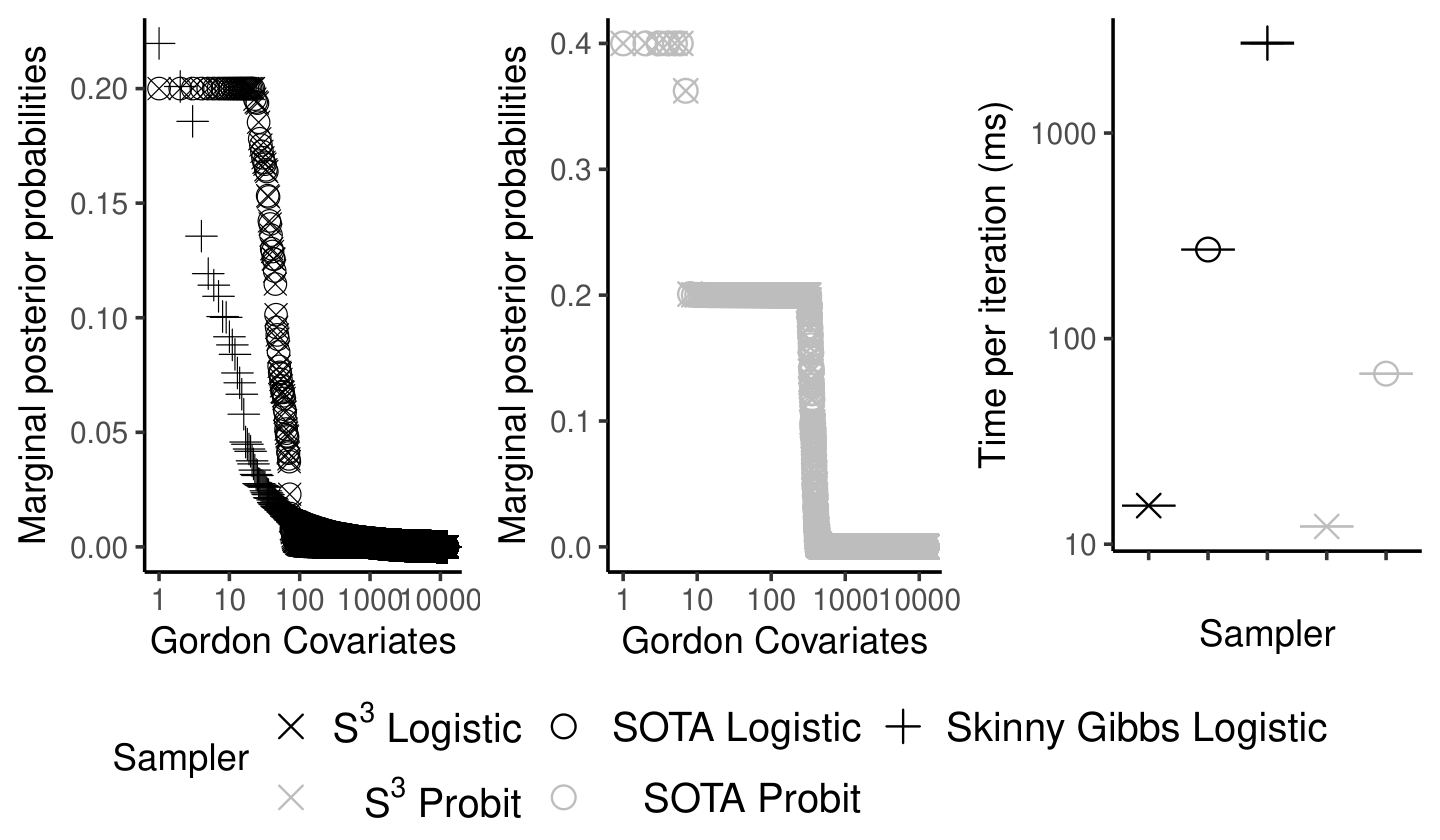
Figure 5, plotted with the y-axis on the log-scale, compares the runtimes of and the SOTA sampler for linear and probit regression on ten regression and binary classification datasets respectively. It plots the average runtimes with one standard error bars based on independent chains each of length and for and the SOTA sampler respectively. Figure 5 shows that has lower runtimes per iteration compared to the SOTA sampler for all the datasets considered, with the most substantial speedups for larger datasets. For example, for the Maize GWAS dataset (Romay et al. 2013; Liu et al. 2016; Zeng & Zhou 2017) with observations (corresponding to average number of days taken for silk emergence in different maize lines) and covariates (corresponding to single nucleotide polymorphisms (SNPs) in the genome), requires ms per iteration on average, which is times faster than the SOTA sampler requiring ms per iteration. For researchers, such speedups can reduce algorithm runtime from days to hours, giving substantial time and computational cost savings at no compromise to inferential quality. Appendix E contains additional results of applied to these datasets including effective sample size (ESS) calculations, marginal posterior probabilities, and performance under 10-fold cross-validation.
5 Further Work
The following questions arise from our work.
Extensions of to point-mass spike-and-slab priors, as well as to non-Gaussian tails. Whilst priors given in (1) are one of the most common formulations employed in practice, a number of alternatives are available. This includes point-mass spike-and-slab priors (Mitchell & Beauchamp 1988; Johnson & Rossell 2012, e.g.,), where a degenerate Dirac distribution about zero is chosen for the spike part, and extensions which consider the heavier-tailed Laplace distribution for the slab part instead of a Gaussian distribution (Castillo et al. 2015; Ročková 2018; Ray et al. 2020; Ray & Szabó 2021). An extension of would to be employ similar pre-computation based strategy of Section 2 to MCMC samplers for these alternative formulations.
Convergence complexity analysis of . An important question that is not addressed in this article is the number of iterations required for or other similar samplers to converge to the their target posterior distributions. For Gibbs samplers targeting posteriors corresponding to continuous shrinkage priors (Carvalho et al. 2010; Bhattacharya et al. 2015; Bhadra et al. 2019, e.g.,), much theoretical progress has been made (Pal & Khare 2014; Qin & Hobert 2019; Bhattacharya et al. 2022; Biswas et al. 2022). Convergence of Gibbs samplers targeting spike-and-slab posteriors has been less extensively studied and requires more attention.
Diagnostics to assess the convergence of and asymptotic variance of . Given some time and computational budget constraints, an immediate benefit of is the ability to run longer Markov chains targeting spike-and-slab posteriors. This can alleviate some concerns linked to burn-in and asymptotic variance, but convergence and effective sample size diagnostics (Johnson 1998; Biswas et al. 2019; Vats & Knudson 2021; Vehtari et al. 2021) remain an important consideration particularly in high-dimensional settings. We hope to investigate convergence diagnostics in future work.
Acknowledgments.
We thank Juan Shen for sharing the PCR and the Lymph Node datasets, Xiaolei Liu and Xiang Zhou for sharing the Maize GWAS dataset, and Marina Vannucci for helpful feedback. NB was supported by the NSF grant DMS-1844695, a GSAS Merit Fellowship, and a Two Sigma Fellowship Award. XLM was partially supported by the NSF grant DMS-1811308.
References
- Banerjee et al. (2021) Banerjee, S., Castillo, I., and Ghosal, S. Bayesian inference in high-dimensional models. Springer volume on Data Science, 2021.
- Barbieri & Berger (2004) Barbieri, M. M. and Berger, J. O. Optimal predictive model selection. Annals of Statistics, 32(3):870 – 897, 2004. doi: 10.1214/009053604000000238. URL https://doi.org/10.1214/009053604000000238.
- Barbieri et al. (2021) Barbieri, M. M., Berger, J. O., George, E. I., and Ročková, V. The Median Probability Model and Correlated Variables. Bayesian Analysis, 16(4):1085 – 1112, 2021. doi: 10.1214/20-BA1249. URL https://doi.org/10.1214/20-BA1249.
- Bhadra et al. (2019) Bhadra, A., Datta, J., Polson, N. G., and Willard, B. Lasso Meets Horseshoe: A Survey. Statistical Science, 34(3):405 – 427, 2019. doi: 10.1214/19-STS700. URL https://doi.org/10.1214/19-STS700.
- Bhattacharya et al. (2015) Bhattacharya, A., Pati, D., Pillai, N. S., and Dunson, D. B. Dirichlet–Laplace Priors for Optimal Shrinkage. Journal of the American Statistical Association, 110(512):1479–1490, 2015. doi: 10.1080/01621459.2014.960967. URL https://doi.org/10.1080/01621459.2014.960967.
- Bhattacharya et al. (2016) Bhattacharya, A., Chakraborty, A., and Mallick, B. K. Fast sampling with Gaussian scale mixture priors in high-dimensional regression. Biometrika, 103(4):985–991, 2016. ISSN 0006-3444. doi: 10.1093/biomet/asw042. URL https://doi.org/10.1093/biomet/asw042.
- Bhattacharya et al. (2022) Bhattacharya, S., Khare, K., and Pal, S. Geometric ergodicity of Gibbs samplers for the Horseshoe and its regularized variants. Electronic Journal of Statistics, 16(1):1 – 57, 2022. doi: 10.1214/21-EJS1932. URL https://doi.org/10.1214/21-EJS1932.
- Biswas et al. (2019) Biswas, N., Jacob, P. E., and Vanetti, P. Estimating convergence of markov chains with l-lag couplings. In Advances in Neural Information Processing Systems, volume 32. Curran Associates, Inc., 2019. URL https://proceedings.neurips.cc/paper/2019/file/aec851e565646f6835e915293381e20a-Paper.pdf.
- Biswas et al. (2022) Biswas, N., Bhattacharya, A., Jacob, P. E., and Johndrow, J. E. Coupling-based convergence assessment of some gibbs samplers for high-dimensional bayesian regression with shrinkage priors. Journal of the Royal Statistical Society: Series B (Statistical Methodology), 2022. doi: 10.1111/rssb.12495. URL https://doi.org/10.1111/rssb.12495.
- Bogdan et al. (2015) Bogdan, M., van den Berg, E., Sabatti, C., Su, W., and Candès, E. J. SLOPE—Adaptive variable selection via convex optimization. The Annals of Applied Statistics, 9(3):1103 – 1140, 2015. doi: 10.1214/15-AOAS842. URL https://doi.org/10.1214/15-AOAS842.
- Carvalho et al. (2010) Carvalho, C. M., Polson, N. G., and Scott, J. G. The horseshoe estimator for sparse signals. Biometrika, 97(2):465–480, 04 2010. ISSN 0006-3444. doi: 10.1093/biomet/asq017. URL https://doi.org/10.1093/biomet/asq017.
- Castillo & van der Vaart (2012) Castillo, I. and van der Vaart, A. Needles and Straw in a Haystack: Posterior concentration for possibly sparse sequences. Annals of Statistics, 40(4):2069 – 2101, 2012. doi: 10.1214/12-AOS1029. URL https://doi.org/10.1214/12-AOS1029.
- Castillo et al. (2015) Castillo, I., Schmidt-Hieber, J., and van der Vaart, A. Bayesian linear regression with sparse priors. Annals of Statistics, 43(5):1986–2018, 2015. doi: 10.1214/15-AOS1334. URL https://doi.org/10.1214/15-AOS1334.
- Dua & Graff (2017) Dua, D. and Graff, C. UCI machine learning repository, 2017. URL http://archive.ics.uci.edu/ml.
- Flegal et al. (2021) Flegal, J. M., Hughes, J., Vats, D., Dai, N., Gupta, K., and Maji, U. mcmcse: Monte Carlo Standard Errors for MCMC. Riverside, CA, and Kanpur, India, 2021. R package version 1.5-0.
- George & McCulloch (1993) George, E. I. and McCulloch, R. E. Variable Selection via Gibbs Sampling. Journal of the American Statistical Association, 88(423):881–889, 1993. doi: 10.1080/01621459.1993.10476353. URL https://www.tandfonline.com/doi/abs/10.1080/01621459.1993.10476353.
- George & McCulloch (1997) George, E. I. and McCulloch, R. E. Approaches for Bayesian Variable Selection. Statistica Sinica, 7(2):339–373, 1997. ISSN 10170405, 19968507. URL http://www.jstor.org/stable/24306083.
- Gordon et al. (2002) Gordon, G. J. G., Jensen, R. V. R., Hsiao, L.-L. L., Gullans, S. R. S., Blumenstock, J. E. J., Ramaswamy, S. S., Richards, W. G. W., Sugarbaker, D. J. D., and Bueno, R. R. Translation of Microarray Data into Clinically Relevant Cancer Diagnostic Tests Using Gene Expression Ratios in Lung Cancer and Mesothelioma. Cancer Research, 62(17):4963–4967, September 2002.
- Guan & Stephens (2011) Guan, Y. and Stephens, M. Bayesian variable selection regression for genome-wide association studies and other large-scale problems. The Annals of Applied Statistics, 5(3):1780 – 1815, 2011. doi: 10.1214/11-AOAS455. URL https://doi.org/10.1214/11-AOAS455.
- Hager (1989) Hager, W. W. Updating the inverse of a matrix. SIAM Review, 31(2):221–239, 1989. ISSN 00361445. URL http://www.jstor.org/stable/2030425.
- Hans et al. (2007) Hans, C., Dobra, A., and West, M. Shotgun Stochastic Search for “Large p” Regression. Journal of the American Statistical Association, 102(478):507–516, 2007. doi: 10.1198/016214507000000121. URL https://doi.org/10.1198/016214507000000121.
- Held & Holmes (2006) Held, L. and Holmes, C. C. Bayesian auxiliary variable models for binary and multinomial regression. Bayesian Analysis, 1(1):145 – 168, 2006. doi: 10.1214/06-BA105. URL https://doi.org/10.1214/06-BA105.
- Ishwaran & Rao (2005) Ishwaran, H. and Rao, J. S. Spike and slab variable selection: Frequentist and Bayesian strategies. Annals of Statistics, 33(2):730 – 773, 2005. doi: 10.1214/009053604000001147. URL https://doi.org/10.1214/009053604000001147.
- Johndrow et al. (2020) Johndrow, J., Orenstein, P., and Bhattacharya, A. Scalable Approximate MCMC Algorithms for the Horseshoe Prior. Journal of Machine Learning Research, 21(73):1–61, 2020. URL http://jmlr.org/papers/v21/19-536.html.
- Johnson (1998) Johnson, V. E. A coupling-regeneration scheme for diagnosing convergence in Markov chain Monte Carlo algorithms. Journal of the American Statistical Association, 93(441):238–248, 1998.
- Johnson & Rossell (2012) Johnson, V. E. and Rossell, D. Bayesian Model Selection in High-Dimensional Settings. Journal of the American Statistical Association, 107(498):649–660, 2012. doi: 10.1080/01621459.2012.682536. URL https://doi.org/10.1080/01621459.2012.682536.
- Johnstone & Silverman (2004) Johnstone, I. M. and Silverman, B. W. Needles and straw in haystacks: Empirical Bayes estimates of possibly sparse sequences. Annals of Statistics, 32(4):1594 – 1649, 2004. doi: 10.1214/009053604000000030. URL https://doi.org/10.1214/009053604000000030.
- Kelly (2007) Kelly, B. C. Some Aspects of Measurement Error in Linear Regression of Astronomical Data. The Astrophysical Journal, 665(2):1489–1506, aug 2007. doi: 10.1086/519947. URL https://doi.org/10.1086/519947.
- Liang et al. (2013) Liang, F., Song, Q., and Yu, K. Bayesian Subset Modeling for High-Dimensional Generalized Linear Models. Journal of the American Statistical Association, 108(502):589–606, 2013. doi: 10.1080/01621459.2012.761942. URL https://doi.org/10.1080/01621459.2012.761942.
- Liu et al. (2016) Liu, X., Huang, M., Fan, B., Buckler, E. S., and Zhang, Z. Iterative Usage of Fixed and Random Effect Models for Powerful and Efficient Genome-Wide Association Studies. PLOS Genetics, 12(2):1–24, 2016. doi: 10.1371/journal.pgen.1005767. URL https://doi.org/10.1371/journal.pgen.1005767.
- Mitchell & Beauchamp (1988) Mitchell, T. J. and Beauchamp, J. J. Bayesian Variable Selection in Linear Regression. Journal of the American Statistical Association, 83(404):1023–1032, 1988. ISSN 01621459. URL http://www.jstor.org/stable/2290129.
- Narisetty & He (2014) Narisetty, N. N. and He, X. Bayesian variable selection with shrinking and diffusing priors. Annals of Statistics, 42(2):789 – 817, 2014. doi: 10.1214/14-AOS1207. URL https://doi.org/10.1214/14-AOS1207.
- Narisetty et al. (2019) Narisetty, N. N., Shen, J., and He, X. Skinny Gibbs: A Consistent and Scalable Gibbs Sampler for Model Selection. Journal of the American Statistical Association, 114(527):1205–1217, 2019. doi: 10.1080/01621459.2018.1482754. URL https://doi.org/10.1080/01621459.2018.1482754.
- O’Brien & Dunson (2004) O’Brien, S. M. and Dunson, D. B. Bayesian multivariate logistic regression. Biometrics, 60(3):739–746, 2004. doi: 10.1111/j.0006-341X.2004.00224.x. URL https://doi:10.1111/j.0006-341X.2004.00224.x.
- Pal & Khare (2014) Pal, S. and Khare, K. Geometric ergodicity for Bayesian shrinkage models. Electronic Journal of Statistics, 8(1):604–645, 2014. doi: 10.1214/14-EJS896. URL https://doi.org/10.1214/14-EJS896.
- Polson et al. (2013) Polson, N. G., Scott, J. G., and Windle, J. Bayesian Inference for Logistic Models Using Pólya–Gamma Latent Variables. Journal of the American Statistical Association, 108(504):1339–1349, 2013. doi: 10.1080/01621459.2013.829001. URL https://doi.org/10.1080/01621459.2013.829001.
- Qin & Hobert (2019) Qin, Q. and Hobert, J. P. Convergence complexity analysis of Albert and Chib’s algorithm for Bayesian probit regression. Annals of Statistics, 47(4):2320–2347, 2019. doi: 10.1214/18-AOS1749. URL https://doi.org/10.1214/18-AOS1749.
- Ray & Szabó (2021) Ray, K. and Szabó, B. Variational bayes for high-dimensional linear regression with sparse priors. Journal of the American Statistical Association, 0(0):1–12, 2021. doi: 10.1080/01621459.2020.1847121. URL https://doi.org/10.1080/01621459.2020.1847121.
- Ray et al. (2020) Ray, K., Szabo, B., and Clara, G. Spike and slab variational bayes for high dimensional logistic regression. In Advances in Neural Information Processing Systems, volume 33, pp. 14423–14434. Curran Associates, Inc., 2020. URL https://proceedings.neurips.cc/paper/2020/file/a5bad363fc47f424ddf5091c8471480a-Paper.pdf.
- Romay et al. (2013) Romay, M. C., Millard, M. J., Glaubitz, J. C., Peiffer, J. A., Swarts, K. L., Casstevens, T. M., Elshire, R. J., Acharya, C. B., Mitchell, S. E., Flint-Garcia, S. A., McMullen, M. D., Holland, J. B., Buckler, E. S., and Gardner, C. A. Comprehensive genotyping of the USA national maize inbred seed bank. Genome Biology, 14(6):R55, 2013. doi: 10.1186/gb-2013-14-6-r55. URL https://doi.org/10.1186/gb-2013-14-6-r55.
- Ročková (2018) Ročková, V. Bayesian estimation of sparse signals with a continuous spike-and-slab prior. Annals of Statistics, 46(1):401 – 437, 2018. doi: 10.1214/17-AOS1554. URL https://doi.org/10.1214/17-AOS1554.
- Scott & Berger (2010) Scott, J. G. and Berger, J. O. Bayes and empirical-Bayes multiplicity adjustment in the variable-selection problem. Annals of Statistics, 38(5):2587 – 2619, 2010. doi: 10.1214/10-AOS792. URL https://doi.org/10.1214/10-AOS792.
- Sereno (2015) Sereno, M. A Bayesian approach to linear regression in astronomy. Monthly Notices of the Royal Astronomical Society, 455(2):2149–2162, 11 2015. ISSN 0035-8711. doi: 10.1093/mnras/stv2374. URL https://doi.org/10.1093/mnras/stv2374.
- Tadesse & Vannucci (2021) Tadesse, M. G. and Vannucci, M. Handbook of Bayesian Variable Selection. Chapman and Hall/CRC, 2021. doi: 10.1201/9781003089018. URL https://doi.org/10.1201/9781003089018.
- Tibshirani (1996) Tibshirani, R. Regression Shrinkage and Selection Via the Lasso. Journal of the Royal Statistical Society: Series B (Statistical Methodology), 58(1):267–288, 1996. doi: 10.1111/j.2517-6161.1996.tb02080.x. URL https://doi.org/10.1111/j.2517-6161.1996.tb02080.x.
- Titsias & Lázaro-Gredilla (2011) Titsias, M. and Lázaro-Gredilla, M. Spike and slab variational inference for multi-task and multiple kernel learning. In Advances in Neural Information Processing Systems, volume 24. Curran Associates, Inc., 2011. URL https://proceedings.neurips.cc/paper/2011/file/b495ce63ede0f4efc9eec62cb947c162-Paper.pdf.
- Vats & Knudson (2021) Vats, D. and Knudson, C. Revisiting the Gelman–Rubin Diagnostic. Statistical Science, 36(4):518 – 529, 2021. doi: 10.1214/20-STS812. URL https://doi.org/10.1214/20-STS812.
- Vats et al. (2019) Vats, D., Flegal, J. M., and Jones, G. L. Multivariate output analysis for Markov chain Monte Carlo. Biometrika, 106(2):321–337, 2019. ISSN 0006-3444. doi: 10.1093/biomet/asz002. URL https://doi.org/10.1093/biomet/asz002.
- Vehtari et al. (2021) Vehtari, A., Gelman, A., Simpson, D., Carpenter, B., and Bürkner, P.-C. Rank-Normalization, Folding, and Localization: An Improved for Assessing Convergence of MCMC (with Discussion). Bayesian Analysis, 16(2):667 – 718, 2021. doi: 10.1214/20-BA1221. URL https://doi.org/10.1214/20-BA1221.
- Yang et al. (2016) Yang, Y., Wainwright, M. J., and Jordan, M. I. On the computational complexity of high-dimensional Bayesian variable selection. Annals of Statistics, 44(6):2497–2532, 2016. doi: 10.1214/15-AOS1417. URL https://doi.org/10.1214/15-AOS1417.
- Zeng & Zhou (2017) Zeng, P. and Zhou, X. Non-parametric genetic prediction of complex traits with latent Dirichlet process regression models. Nature Communications, 8(1):456, 2017. doi: 10.1038/s41467-017-00470-2. URL https://doi.org/10.1038/s41467-017-00470-2.
- Zhou et al. (2013) Zhou, X., Carbonetto, P., and Stephens, M. Polygenic Modeling with Bayesian Sparse Linear Mixed Models. PLOS Genetics, 9(2):1–14, 02 2013. doi: 10.1371/journal.pgen.1003264. URL https://doi.org/10.1371/journal.pgen.1003264.
- Zou & Hastie (2005) Zou, H. and Hastie, T. Regularization and variable selection via the elastic net. Journal of the Royal Statistical Society: Series B (Statistical Methodology), 67(2):301–320, 2005. doi: 10.1111/j.1467-9868.2005.00503.x. URL https://doi.org/10.1111/j.1467-9868.2005.00503.x.
Appendix A Proofs
Proof of Proposition 2.1.
Consider Step of Algorithm 2 and Algorithm 3 for probit regression. Given pre-computed matrices , , , and state , calculating , requires cost by (3) and (4), where for .
Consider Step of Algorithm 3 for logistic regression. This requires cost, where the cost arises from the calculation of using (21) and the cost arises from inverting to calculate .
Given , Step of Algorithms 2 and 3 then requires cost, which arises from the matrix vector product for in Algorithm 1. By component-wise independence, Step of Algorithms 2 and 3 costs and Step of Algorithm 3 cost . Step of Algorithm 3 and Step of Algorithm 3 for probit regression both cost . Step of Algorithm 3 for logistic regression both costs .
Proof of Proposition 2.2.
By linearity, where for each component the random variables and are on . For each , we obtain
When follows the stationary , and . Consequently,
∎
Appendix B Algorithm Derivations
B.1 Linear regression with spike-and-slab priors
B.2 Probit regression with spike-and-slab priors
Consider the probit regression likelihood, where for each observation , for the -th row of the design matrix . and that cumulative density function of a univariate Normal distribution. We obtain for . The Bayesian probit regression model is then given by
| (15) | ||||
For the prior and likelihood in (15), the posterior density of is given by
| (16) |
From (16), we can calculate the conditional distributions. We obtain
as required for probit regression in Algorithm 3.
B.3 Logistic regression with spike-and-slab priors
We first describe the Bayesian logistic regression model considered. Consider the logistic regression likelihood, where for each observation , for the -th row of the design matrix . We obtain where , corresponding to the logistic distribution centered about and scale parameter .
B.3.1 Student’s -distribution based approximation of the logistic regression likelihood.
Following O’Brien & Dunson 2004 and Narisetty et al. 2019, we can approximate with , where denotes a -distribution with degrees of freedom and is a multiplicative factor. The constants and are chosen following O’Brien & Dunson 2004, in order to match the variance of the logistic distribution and to minimize the integrated squared distance between the respective densities. The Gaussian scale representation of this -distribution is
| (17) |
where each is an augmented variable. The Bayesian logistic regression model is then given by
| (18) | ||||
Let denote the vector with entries for . For the prior and likelihood in (18), the posterior density of on is given by
| (19) |
From (19), we can calculate the conditional distributions. Let . We obtain
as required for logistic regression in Algorithm 3.
A scalable Gibbs sampler for logistic regression.
The computational bottleneck of existing Gibbs samplers for logistic regression is linked to sampling from the full conditional of . This is given by
| (20) |
where indexes the iteration of the Markov chain, is the diagonal matrix with the vector populating its diagonal elements, and is the diagonal matrix with the vector populating its diagonal elements. To sample from (20), we can use the sampler of Bhattacharya et al. 2016, which is given in Algorithm 4.
| Following the strategy in Section 2.2, for logistic regression uses pre-computation to reduce the computational cost of Algorithm 4. Using the notation from Section 2.2 with , we note | ||||
| (21a) | ||||
| (21b) | ||||
| (21c) | ||||
| In (21a) – (21c), calculating the matrix products , , and requires , , and cost respectively. Given , , , and , we evaluate whichever matrix product in (21a) – (21c) has minimal computational cost and thereby calculate at the reduced cost of where . | ||||
To calculate , we calculate by directly inverting the calculated matrix , which requires cost. Overall, this strategy reduces the computational cost of calculating the matrices and from to .
Extensions to Scalable Spike-and-Slab for logistic regression.
Suppose the matrices is pre-computed. This initial step requires computational cost and memory. Then the matrices and in (21a) – (21b) correspond to pre-computed sub-matrices of , and calculating using (21a) – (21b) each iteration involves matrix addition and diagonal matrix multiplication which only requires cost. To sample from (20), we calculate by directly inverting the calculated matrix from (3), which requires cost. Overall, now the Gibbs samplers for logistic regression requires computational cost at iteration , which is an improvement compared to .
Appendix C Experiment Details
Figure 3 of Section 3.
In Figure 3, we use the same prior hyperparameters for all the algorithms. Following Narisetty et al. 2019, we choose , and such that for . The true positive rate (TPR) and the false discovery rate (FDR) correspond to the proportion of non-zero and zero components of that are correctly selected respectively. They are calculated as and respectively, where the marginal posterior probabilities are estimated by for sample points generated using or Skinny Gibbs. The lines in Figure 3 correspond to the average TPR and FDR across independently generated datasets, and the grey bands correspond to one standard error of the averages.
Appendix D Dataset Details
Synthetic continuous response dataset in Section 2.3.
In Figure 1, synthetic linear regression datasets are considered. For number of observations and number of covariates , we generate a design matrix such that each for all and , which is then scaled to ensure each column has a mean of and a standard error of . We choose the true signal such that , where is the sparsity parameter corresponding to the number of non-zero components. Given and , we generate for , where is the Gaussian noise standard deviation.
Synthetic binary response dataset in Section 3.
In Figures 2 and 3, synthetic binary classification datasets are considered. For number of observations and number of covariates , we generate a design matrix such that each for all and , which is then scaled to ensure each column has a mean of and a standard error of . We choose the true signal such that , where is the sparsity parameter corresponding to the number of non-zero components. Given and , we generate for for , where is the -th row of and is the Logistic distribution with mean and scale parameter .
Datasets in Section 4.
The Malware detection dataset from the UCI machine learning repository (Dua & Graff 2017) has observations with binary responses and covariates, and is publicly available on www.kaggle.com/piyushrumao/malware-executable-detection.
The Borovecki, Chowdary, Chin and Gordon datasets are all high-dimensional microarray datasets. They are publicly available on the package in . The Borovecki dataset has observations with binary responses and covariates. The Chowdary dataset has observations with binary responses and covariates. The Chin dataset has observations with binary responses and covariates. The Gordon dataset has observations with binary responses and covariates.
The PCR GWAS dataset has observations with continuous responses and covariates, and is publicly available on www.ncbi.nlm.nih.gov/geo (accession number ). The Lymph Node GWAS dataset has observations with binary responses and covariates, and has been previously considered (Hans et al. 2007; Liang et al. 2013; Narisetty et al. 2019). The Maize GWAS dataset has observations with continuous responses and covariates, and has been previously considered (Romay et al. 2013; Liu et al. 2016; Zeng & Zhou 2017). The Lymph Node GWAS and the Maize GWAS datasets are not publicly available.
The synthetic continuous dataset has observations and covariates. The design matrix is generates such that each for all and , which is then scaled to ensure each column has a mean of and a standard error of . The true signal is chosen such that , where is the sparsity parameter corresponding to the number of non-zero components. Given and , we generate for , where is the Gaussian noise standard deviation. The synthetic binary classification dataset is generated as in Section 3, with observations and covariates.
Appendix E Additional Experiments
Variable selection performance as a function of time or number of iterations.
Figure 6 plots the average true positive rate (TPR) and the false discovery rate (FDR) of variable selection based on samples from and Skinny Gibbs as the length of the chains are varied. The TPR and FDR are averaged over independent chains, and one standard error bars are shown. We consider a synthetic binary classification dataset generated using a logistic regression model as in Section 3, with observations, covariates, sparsity , and an exponentially decaying sparse true signal such that for and for . The TPR and FDR are calculated as in Section 3 with the marginal posterior probabilities now estimated by for a burn-in of , a varying chain length , and sample points generated using or Skinny Gibbs. We use the same prior hyperparameters for all the algorithms, which are chosen according to Narisetty et al. 2019.
Figure 6 Left and Center-Left plot the TPR and FDR against the chain length . It shows that for both logistic and probit regression have higher TPR and lower FDR than Skinny Gibbs for all chain lengths. Furthermore, for logistic regression has higher TPR and lower FDR than for probit regression, which is expected as the synthetic dataset for this example is generated using a logistic regression model. The SOTA sampler is omitted from the Left and Center-Left plots as its output has the same marginal distribution and statistical performance as . Figure 6 Center-Right and Right plot the TPR and FDR against total time elapsed in seconds to generate samples using , SOTA, or Skinny Gibbs chains with a burn-in of iterations. The standard error bars are now omitted for better visibility. For each time budget, we observe better variable selection performance from when compared with the slower SOTA implementation or with Skinny Gibbs.
Effective Sample Size of for the datasets in Section 4.
Figure 7 shows the Effective Sample Size per iteration and per unit of time (in seconds) of and the SOTA sampler for the datasets in Section 4. The ESS is calculated using the package (Flegal et al. 2021; Vats et al. 2019) for one chain of length iterations with a burn-in of iterations for each dataset. The average ESS of the components are then plotted. Figure 7 Right shows that has significantly higher ESS per second compared to the corresponding SOTA sampler for all the datasets considered.
Performance metrics for the datasets in Section 4.
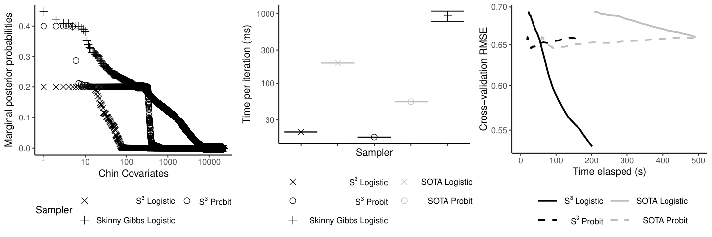
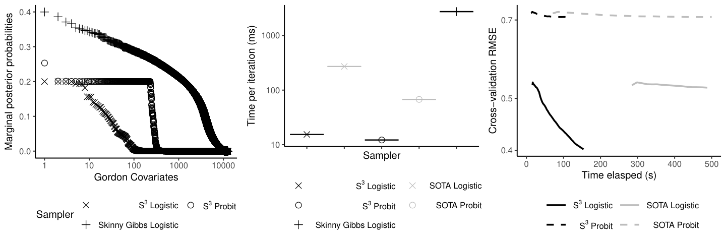
Figures 8 – 14 show various performance metrics of for some of the datasets considered in Section 4. Figures 8 – 14 (Left) plot the marginal posterior probability estimates against in the decreasing order of s, following the setup in Figure 4. For datasets with continuous valued responses, s are based on samples from for linear regression. For datasets with binary valued responses, s are based on samples from for logistic and probit regression, and the Skinny Gibbs sampler from logistic regression. We use samples from independent chains of length iterations with a burn-in of iterations. Estimates based on samples from the SOTA sampler are not shown, as they implement the same Gibbs sampler as (other than possible numerical discrepancies, as discussed in Section 4).
Figures 8 – 14 (Center) show the average time taken per iteration with one standard error bars for , the SOTA sampler, and the Skinny Gibbs sampler based on independent chains of length iterations.
Figures 8 – 14 (Right) show the 10-fold cross-validation average root-mean-square error (RMSE) against the total time elapsed to run one and one SOTA chain. To compute this evaluation, we partition the observed dataset into folds uniformly at random and, for each fold , run a chain conditioned on all data outside of fold and evaluate its performance on the held-out data in the -th fold. The average RMSE is calculated as , where is the RMSE for the fold. For datasets with continuous valued responses, the quantities for linear regression are calculated as where is the fold, are the predicted responses, and are samples from and SOTA targeting the posterior distribution of the training set. For datasets with binary valued responses, the quantities are calculated as , where is the fold, and are the predicted probabilities for logistic and probit regression respectively, and are samples from and SOTA targeting the posterior distribution of the training set. Figures 8 – 14 (Right) plot the average RMSE against total time elapsed in seconds to generate samples using or SOTA chains with a burn-in of iterations. The RMSE of the Skinny Gibbs sampler is not available, as the package does not output the full chain trajectories required for RMSE calculations.