A PRticle filter algorithm for nonparametric estimation of multivariate mixing distributions
Abstract
Predictive recursion (PR) is a fast, recursive algorithm that gives a smooth estimate of the mixing distribution under the general mixture model. However, the PR algorithm requires evaluation of a normalizing constant at each iteration. When the support of the mixing distribution is of relatively low dimension, this is not a problem since quadrature methods can be used and are very efficient. But when the support is of higher dimension, quadrature methods are inefficient and there is no obvious Monte Carlo-based alternative. In this paper, we propose a new strategy, which we refer to as PRticle filter, wherein we augment the basic PR algorithm with a filtering mechanism that adaptively reweights an initial set of particles along the updating sequence which are used to obtain Monte Carlo approximations of the normalizing constants. Convergence properties of the PRticle filter approximation are established and its empirical accuracy is demonstrated with simulation studies and a marked spatial point process data analysis.
Keywords and phrases: importance sampling; marked point process; mixture model; Monte Carlo; predictive recursion.
1 Introduction
Suppose we have independent and identically distributed (iid) data having common density supported on . Furthermore, suppose that we believe this density has the mixture form , where
| (1) |
with a known kernel density and an unknown mixing distribution supported on . The family in (1) indexed by is commonly referred to as a mixture model. One interpretation of the mixture model is that there is a set of underlying latent variables driving the data-generating process. That is, suppose the ’s are obtained through the two-step process:
It is easy to check that from this hierarchical model formulation are iid with density . This sort of hierarchical, latent variable modeling is common when heterogeneity is present in the observed data. This also covers the class of problems where represents an unobservable “signal” of interest and the corresponding noise-corrupted signal, i.e., the “signal plus noise.” One also might adopt (1) simply for the flexibility the mixture model affords (e.g., DasGupta, 2008, Chapter 33). In any case, the distribution of the latent variables, or signals, may be of some practical interest, in which case the goal becomes estimation of the unknown mixing distribution based on iid data from the mixture in (1). This is our focus in the present paper.
Estimation of the mixing distribution is a notoriously difficult problem. Aside from methods tailored to specific mixture model forms, e.g., deconvolution (Fan, 1991; Stefanski and Carroll, 1990), there are a few general estimation methods available: the two “standard” approaches are nonparametric maximum likelihood and nonparametric Bayes. The former maximizes the likelihood based on observations from , with respect to . Given the nonparametric nature of , the resulting estimate is almost surely discrete and the points of support are no greater than (Lindsay, 1983). The latter approach assigns a prior distribution to , typically a Dirichlet process (Ghosh and Ramamoorthi, 2003; Ghosal and Van der Vaart, 2017; Hjort et al., 2010; Ferguson, 1974), and evaluate the corresponding posterior mean, given . Even though there is no direct imposition of discreteness in the posterior, draws from the posterior distribution of have atoms (Blackwell and MacQueen, 1973, e.g.,) and the corresponding posterior mean is spiky, “effectively discrete.” Hence, neither the likelihood nor Bayesian approaches give satisfactory solutions to the problem of estimating a mixing distribution in (1). The point is that, in these traditional approaches, the focus is on identifying candidate such that resulting mixture density is compatible with the empirical distribution of data, not specifically estimating the mixing distribution.
A third general approach is available, which is the primary focus of this paper, called predictive recursion (PR). Unlike the previous two methods, which are likelihood-based, the PR estimator is based on a stochastic, recursive algorithm that aims specifically to estimating the mixing distribution based on data from the mixture model (1). This strategy was first proposed in Newton et al., 1998 as a fast and smooth approximation to the posterior mean of under a Dirichlet process mixture model; see Martin, 2021. The idea behind PR is to start with a initial guess, , and then update that guess recursively based on each individual observation for . PR has a number of desirable computational and statistical properties. First, PR is computationally efficient—its complexity is . Second, the PR estimator, , is absolutely continuous with respect to , so if has a smooth density, then so does . Third, the PR estimator has also been shown to consistently estimate the true mixing distribution in a series of papers: Tokdar et al., 2009, Martin and Tokdar, 2009, and Dixit and Martin, 2021.
Applications of the PR algorithm have appeared in Newton, 2002, Martin and Tokdar, 2011, Martin and Tokdar, 2012, Martin and Han, 2016, Tansey et al., 2018, Woody et al., 2022, and Dixit and Martin, 2022. In each of these applications, however, the mixing distribution support is a relatively low-dimensional space, e.g., one- or two-dimensional. The reason for this constraint is that, while the algorithm itself is completely general, computation of the normalizing constant in Equation (2) below can be a challenge when is more than two- or three-dimensional. In particular, the required integration can only be done numerically, but efficient quadrature methods are available only when the domain of integration, in this case , is low-dimensional. A Monte Carlo-based strategy would be less sensitive to the dimension of and, in that sense, would have an advantage. Unfortunately, no such Monte Carlo-based strategy is currently available in the literature, and this paper aims to fill this gap.
Following a brief review in Section 2 of the PR algorithm and importance sampling techniques, we propose in Section 3 below the PRticle filter approximation. As the name suggests, this consists of an augmentation of the original PR algorithm with a filtering step that adaptively reweights an initial set of particles along the PR updating sequence. The idea is that, at the step, the weighted set of particles resembles a sample from the PR estimate based on data . Hence, the step gives a particle approximation of the PR estimate and Theorem 1 below establishes that, for fixed data , this approximation converges almost surely in total variation distance to as the number of sampled particles approaches infinity.
In Section 4, we evaluate performance of the proposed PRticle filter approximation on both real and simulated data sets. For the simulated data sets, the evaluation is split into two types. First, to judge the accuracy of the proposed PRticle filter approximation, we compare it to the original PR estimator in cases where a quadrature scheme is feasible. In our comparisons, the PRticle filter accurately approximates the PR estimate for simulations from mixtures corresponding to univariate and bivariate mixing distributions. Second, when the dimension of the mixing distribution support is too large for a quadrature scheme to be practical, we compare our PRticle filter approximation to a Dirichlet process mixture model-based estimator. The PRticle filter approximation is faster to compute and of comparable quality compared to the nonparametric Bayes estimator, which is one of the best known solutions.
For a real data illustration, we consider an application where data consists of a marked spatial point process. That is, the observed data consists of spatial locations at which specific events take place, along with some other relevant feature of the events, called marks. As is common in spatial point process models, the relevant quantity is the intensity function. Here we follow Taddy and Kottas, 2012 and model this intensity function as a mixture, with a multivariate mixing distribution support, and apply the PRticle filter approximation to estimate the mixing distribution and, in turn, the intensity function. This naturally leads to estimates of other relevant features, including conditional distribution of the marks given the spatial locations. We argue that the results obtained through our use of the PRticle approximation are consistent with patterns seen in the data and with those presented elsewhere in the literature. This application simply would have been impossible using the basic PR algorithm. Some concluding remarks are given in Section 5 and the proof of Theorem 1 is presented in Appendix A.
2 Background
2.1 Predictive recursion
Suppose we have data from in (1), where the goal is estimation of the mixing distribution . With a user-defined initial guess and weight sequence , the step in the PR algorithm is given by,
| (2) |
For theoretical reasons, the weights must satisfy and ; this can be achieved by taking, e.g., for some . The algorithm processes the data points sequentially and returns the final update as the PR estimator of the mixing distribution. The corresponding PR mixture density estimate is , where the mapping is given in (1). It is clear that the PR estimator depends on the ordering of the observations . If this dependence is undesirable, then it can be removed—or at least mitigated—by calculating over multiple permutations of the data and averaging over the estimates (Newton, 2002; Tokdar et al., 2009). With the superior computational efficiency of PR, this permutation-averaging can still be carried in a fraction of the run-time of its competitors.
Key features of the PR algorithm/estimator include its ability to estimate a mixing density and its computational efficiency. By the former, we mean that if the user-defined initial guess has a smooth density with respect to a particular dominating measure, then the final PR estimator will too. Compare this to the maximum likelihood and Bayes estimators, which are necessarily (or “effectively”) discrete. By the latter computational efficiency claim, we mean that each PR step requires a fixed number of computations, so the overall computational complexity of PR algorithm is .
As mentioned in Section 1, the key step in each iteration of the PR algorithm is calculation of the normalizing constant . Since is data-driven and fully nonparametric, we cannot expect there to be a closed-form expression for the normalizing constant. Often it can be approximated numerically using a quadrature scheme; this is especially easy to do so when the mixing distribution support is univariate. However, for as the dimension of increases, computation of the normalizing constant becomes more and more challenging. For example, the number of grid points required for accurate quadrature grows exponentially in the dimension of and becomes infeasible or at least inefficient even for moderate . This creates a computational bottleneck.
In previous work, this challenge was side-stepped by treating some of the latent variables as mixing variables and the others as non-mixing/structural parameters. For example, instead of mixing the kernel over both the location and scale , the proposal in Martin and Tokdar, 2011 was to treat, say, the scale parameter as a fixed unknown, so that mixing is required only over the univariate -space. Then they developed a PR-based marginal likelihood for that could be used for simultaneous estimation of the scale and the corresponding mixing distribution over . This effectively reduces the dimension of the mixing distribution support, thus making it easy to side-step the challenges in computing the normalizing constant. For various reasons, however, it would be preferable to deal with the computational challenges directly, as opposed to using a “hack” to reduce the dimension artificially. This requires new ideas for evaluating the normalizing constant in (2) and, for this, here we develop a novel strategy based on the same ideas behind sequential importance sampling.
2.2 Importance sampling and filtering
The approximation we propose in Section 3 uses the principles behind importance sampling and particle filters in general. Before stating our algorithm, we first review these basic principles. Consider the general problem of integrating a function with respect to a probability density , where , for . In cases where numerical integration is infeasible, e.g., if is too large or if either or is too rough, it is common to use a Monte Carlo approximation by averaging over a random set of observations from probability density . However, a problem arises if cannot be efficiently sampled from. In such cases, an importance sampling approach can be employed. This amounts to generating samples from a different distribution, say with density , and then reweighting those samples so that they resemble samples from . In particular, the expected value of with respect to can be written as
and this immediately suggests the Monte Carlo approximation
where are iid samples from and are the weight adjustment factors. If the normalizing constant for is unknown, then the factor can be replaced by .
The ratio helps to effectively filter out points in low -density regions while increasing the weight put on particles in high -density regions. Agapiou et al., 2017 unify the existing literature on importance sampling with a special focus on determining the size of such that error in approximation is minimized. The choice of , the Monte Carlo sample size, is important, both in terms of accuracy and efficiency. A practical measure of efficiency used for importance sampling is the effective sample size (ESS), i.e., the effective number of particles. Following Kong, 1992, a commonly used expression for ESS is
| (3) |
where as before. By Cauchy–Schwartz, ESS is bounded above by , and the closer it is to the more efficient the importance sampler. So the goal is to choose the proposal density such that ESS is as close to as possible.
These basics behind importance sampling can be connected to more sophisticated Monte Carlo methods with the following interpretation. The procedure above essentially starts with a collection of tentative sample points from , which are commonly referred to as particles. Particles which have small importance ratios, , are given small weight, and effectively filtered out. In this sense, importance sampling is a (basic) form of particle filtering. This idea can then be extended in different directions. In particular, it would be possible for the target distribution, , to be changing over some “time” index. In hidden Markov models, for example, the dimension of the target distribution’s support is increasing with time; also, in Bayesian inference, the target is the posterior distribution which is evolving with the sample size . Sequential Monte Carlo methods have proved useful in these problems (Doucet et al., 2001; Doucet and Johansen, 2011; Del Moral et al., 2006, e.g.,). Sequential importance sampling, in particular, is a powerful tool for particle filtering (Agapiou et al., 2017; Tokdar and Kass, 2010). In the context of mixture models, sequential importance sampling (MacEachern et al., 1999, eg.) and particle learning algorithms (Carvalho et al., 2010b, eg.) have been suggested for analyzing mixture models in the Bayesian setting. In our present case, sequential updating is required because we need particles that represent the PR estimate as . This problem is due to the unique recursive structure inherent in the PR sequence of target distributions and, therefore, calls for different or at least more specialized techniques compared to what is currently available in the sequential Monte Carlo literature.
3 PRticle filter approximation
3.1 Algorithm
In this section we propose a particle filter algorithm designed specifically to approximation the PR estimator. For simplicity, and without any real loss of generality, assume that has a density with respect to Lebesgue measure on , denote by . Then all the subsequent PR updates have such a density, denoted by . At each iteration of PR, one needs to calculate a normalizing constant
The analytical form of is unknown so clearly we cannot evaluate this in closed form. Likewise, we cannot directly generate observations from it to get a Monte Carlo approximation. However, we know that it is a function of the previous updates , so the idea is to leverage the PR algorithm’s recursive formulation and those core importance sampling principles to design an efficient Monte Carlo/particle filter approximation.
Recall that is a user-specified density on and we will assume that sampling from is feasible. Generate an iid sample of size from . Then, a simple Monte Carlo average gives us an approximation of the first normalizing constant,
where each point is equally weighted by . Next, we do not know the form of but we know that it can be expressed in terms of and the data point as
This implies the ratio of consecutive PR density estimates is
Now, since
we have a very natural Monte Carlo approximation of , namely,
where is based on plugging in for in the definition of above. Here acts as a mesh that effectively filters out those particles that are not compatible with the updated distribution . Continuing with the same logic, for the iteration, we get
where and
The above steps make up the PRticle filter approximation and these are summarized in Algorithm 1. In the end, the algorithm returns the pairs that collectively represent an approximate sample from the PR estimator . From this sample, any features of can be approximated as usual. If an estimate of the density were required, then the weighted collection of particles can be smoothed using, e.g., a kernel density estimator. Just like the PR estimator, the PRticle filter approximation depends on the ordering of observations, and same permutation-averaging can be used here to mitigate the order-dependence, if desired.
3.2 Convergence
A relevant question would be of the convergence of the PRticle filter approximation to the corresponding PR estimate , as the Monte Carlo sample size goes to . If we had just one data point , then simply by the law of large numbers as this only involves the simple Monte Carlo approximation of . However, as we include more observations, the approximation of consists of the previous approximations and the law of large numbers argument is not immediately clear. But it turns out that the law of large numbers can be applied to show that PRticle filter approximation, , converges to its target in a very strong sense as .
Theorem 1.
For a fixed data set , let and denote the PR estimator and its PRticle filter approximation, respectively, both based on the same initial guess with distribution . If the kernel is such that
| (4) |
then
Proof.
See Appendix A. ∎
Theorem 1 establishes that, with a sufficiently large Monte Carlo sample size , the PRticle filter approximation, , of the PR mixing density estimator will be quite accurate. Note that /total variation convergence implies weak convergence, so virtually any relevant functional of can be accurately approximated by the corresponding functional of . The condition (4) on the kernel is rather mild, e.g., it is satisfied if is bounded for almost all . Beyond the fixed-data approximation, the result in Theorem 1, together with the general results in Martin and Tokdar, 2009 and Dixit and Martin, 2021 on the consistency properties of as , suggests that would also be a good estimator of when both and are large.
3.3 Adaptation to handle attrition
The final estimate will depend on the initial , not just through the default PR mechanism but also through the dependence on the choice of particles from . To ensure that captures the true mixing density , it is generally recommended to choose a relatively diffuse in the PR algorithm. However, the true is likely to be more concentrated in certain regions of than in others. So those chosen particles from that happen to fall in those -low-density regions of should be assigned relatively low weights. The concern is that too many of the particles end up in these low-density regions, hence affecting the effective number of particles. Recall that, an efficiency measure of the particle filter is given by the effective sample size (ESS) in (3). For our case this can be calculated as,
If too many particles end up with negligible weights, i.e., if for ’, then ESS becomes significantly smaller than . This loss-of-information, called attrition, is a common problem in importance sampling or particle filtering (Doucet and Johansen, 2011, eg.); and it cannot be ignored because the effective sample size is what controls the accuracy of the Monte Carlo approximations. To account for this, the general strategy is to resample points from the region of importance such that ESS does not reduce tragically (Carvalho et al., 2010b; Doucet et al., 2001, e.g.,). The strategy we propose here is in the same spirit as adaptive importance sampling (Bugallo et al., 2017, eg.). Below we describe our approach that accounts for attrition, specific to the PRticle filter. We start by summarizing the characteristics of the final PR estimate to improve upon the initial filter . This summary can then be used to construct a new informed so that an updated filter has more points in the more dense regions of .
Given points and the final weights representing the PR estimate we can easily obtain Monte Carlo approximations of
the mean vector and covariance matrix associated with , respectively, given by
This helps us to identify a region where —and likely as well— has high concentration. This information can then be incorporated in a new updated . A reasonable strategy, therefore, is to redefine the initial estimate to be, e.g., a multivariate Student-t distribution with location and scale matrix . An iid sample is then generated from this new and the PRticle procedure is carried out as before.
This idea of updating the PRticle filter can be extended in various ways. One way is to repeat the aforementioned process more than once. However, in our experience, this can lead to shrinkage of the region of interest beyond of what is needed resulting into points from only a highly dense region and no points elsewhere. Alternatively, one could identify several particles having relatively large weight following the initial pass of PRticle filter; use these as locations around which a multivariate Gaussian or Student-t distribution could be centered; and then take the updated to be a mixture of these few distributions and sample particles from there. Yet another strategy is to resample particles from after one run of PR and rerun the algorithm by replacing the low-weight particles by the new particles. This allows for identifying new regions of interest while removing any low-probability regions. This is a classical strategy of resampling used in particle filters for Bayesian problems (Carvalho et al., 2010a). Any of the approaches suggested above would be useful in reducing attrition of particles, but more deliberation is needed to conclude which of these strategies would be most efficient. For our purposes here, we use the strategy mentioned before and our simulation results in Section 4 show that this is effective in reducing attrition.
4 Numerical results
4.1 Density estimation
Here we show three density estimation examples. Examples 1–2, involving Euclidean data and data on a sphere, respectively, compare the PRticle filter approximation to the original PR estimator in low-dimensional cases where the latter can be computed efficiently. Example 3 considers cases where the mixing distribution support is too high-dimensional to compute the original PR estimator, so we compare the PRticle filter approximation results to those of the Dirichlet process mixture model fit.
Example 1.
For -dimensional data , consider a normal mixture model of the form (1) with the multivariate normal density with mean vector , where is the -dimensional identity matrix. Throughout, will be taken as fixed. So that we can compare the PRticle filter approximation directly to the original PR estimator, we consider only the cases and here. For the case, we take the true mixing distribution to be , a beta distribution scaled to ; for the case, we take , a joint distribution supported on corresponding to independent scaled beta marginals. In both cases, samples of size are generated and we compare the PRticle filter approximation to the original PR estimator in terms of the Kullback–Leibler divergence , where is the PR estimator of the mixture density and is the corresponding PRticle filter approximation. Both are based on weight sequence and initial guess . The PRticle filter approximation relies on samples taken from and here we consider four samples sizes, . Table 1 summarizes both the Kullback–Leibler divergence and the ESS for both the and cases. As expected, the ESS tends to be smaller for than for , with the former retaining about 15% of the original sample while the latter retains about 33%. However, the Kullback–Leibler divergence tends to be small across the board and does not vary much as a function of for both cases.
|
|
Example 2.
Next, following Dixit and Martin, 2022, we compare the PRticle filter approximation to the original PR estimate for mixture models on the unit sphere commonly used for directional data. The particular mixture model we consider is one with a so-called angular Gaussian distribution (Tyler, 1987) kernel
where , with and is the rotation matrix mapping onto the unit vector , given by
and is the spherical coordinate representation of . For the original PR estimator, Dixit and Martin, 2022 treated as a fixed unknown structural parameter, not a latent variable being mixed over. That is, they treated the kernel as , depending on the unknown , where is the only latent variable mixed over. Then they employed the PR marginal likelihood strategy to estimate the fixed unknown . Here, using the added flexibility of the PRticle filter approximation, we fit the model that mixes over latent variable , so that there are no unknown structural parameters to be estimated separately. Here we generate samples from the above mixture model where the true mixing distribution has a smooth bimodal density in and a point mass at —this means that PR’s mixture model, that takes fixed and unknown, is correctly specified while the PRticle filter’s mixture model is misspecified. For the PR estimator, we take and to be uniform on . For the PRticle filter approximation, which mixes over both and , the initial guess is a product of uniform distributions on and a uniform distribution on . Plots of the PR estimate and PRticle approximation , based on initial particles, are provided in Figure 1. The approximation based on PRticle filter clearly captures all the relevant features of the PR estimate, and in much less time thanks to not needing to employ the marginal likelihood strategy to estimate a fixed .


Example 3.
For the third part of the simulation study, we mix a bivariate normal kernel over all mean and covariance parameters. This means that the mixing distribution is defined over five variables. Using PR with numerical integration is not possible in this situation as a quadrature scheme is infeasible. The PRticle filter approximation can instead be used to fit this mixture density. For comparison, we consider a Dirichlet process mixture model fit, where the prior for the mixing distribution is , a Dirichlet process with precision parameter and base measure , which we take to be the same as PR’s initialization (see below). The Dirichlet process mixture model estimate of the mixture density is the corresponding posterior mean, which is calculated using the DirichletProcessMvnormal function in the R package dirichletprocess (Ross and Markwick, 2019) with 1000 iterations. To compare the two approaches we take with the true mixing distribution corresponding to independent , , , , and . In this, we generate observations from the true mixture density and fit a multivariate normal mixture density using the PRticle filter approximation and the Dirichlet process mixture model machinery. As before we initialize the PRticle filter with a uniform distribution over all parameters and a weight sequence . However, to avoid possible attrition we improve the filter by using the strategy proposed in Section 3.3 and rerun the algorithm with an updated . Contour plots of the estimated mixture densities are given in Figure 2. The PRticle filter approximation plots are able to capture the structure of the true mixture density, , just like the Dirichlet process mixture model fit. For a numerical comparison we calculate the Monte Carlo approximation of the Kullback–Leibler divergence between the true mixture density and the estimated density. This is for a comparison between and while it is for a comparison between and . The Dirichlet process estimate performs slightly better than PR for mixture density estimation, but it is important to note that PR is solving the harder problem of estimating a multivariate mixing density, which the Dirichlet process mixture formulation struggles with because the resulting estimator is effectively discrete. To illustrate this, we draw independent samples of from the true mixing distribution and both the PRticle filter and Bayes estimates of , and display quantile–quantile plots for comparison in Figure 3. The PR quantiles match the true distribution quantiles much more closely compared to the Dirichlet process-based Bayes estimator quantiles. Computationally, fitting of the Dirichlet process mixture takes almost four minutes on our machine, while the PRticle filter approximation is calculated in about one minute.
4.2 Marked point process modeling
Here we showcase an interesting application of multivariate mixture modeling using PR, which is made possible by the PRticle filter approximation. Suppose our data consists of spatial locations of an interesting occurrence possibly accompanied by some attributes at those locations. Typically, when only location observations are available, there is interest in the intensity of the incident occurrence. These are typically modeled as realizations from a non-homogeneous Poisson process with intensity function , (Liang et al., 2008, e.g.). For example, in an epidemiological study, might be the geographic location of the individual showing symptoms of a particular disease and hence there is interest in modeling the intensity of the disease occurrences. For such a non-homogeneous Poisson process, a likelihood function can be written as,
where is the normalized intensity function, i.e., , and . Given the separable nature of the likelihood above, and can be estimated separately. A regression approach is to model by a log Gaussian Cox process (Liang et al., 2008, e.g.). However given the nonparametric nature of the problem it is desirable to use a robust model for to capture all the shape/scale features of the function. Mixture models offer this flexibility and an approach to modeling or by a Dirichlet process mixture was proposed in Kottas and Sansó, 2007.
Additionally, there could be other attributes present with the location data, for example, indicator variable for type of disease, when there is interest in the association between disease locations. Then to account for this association and its effect on the model, a joint intensity function can be defined. The resulting process is known as the marked point process, where the attributes are called marks. The nonparametric mixture density in (1) offers the required flexibility to model a fully nonparametric function . Taddy and Kottas, 2012 propose mixture models for such marked point processes using conditionally conjugate Dirichlet process mixture models. The idea is to model the joint intensity of the locations and marks as,
| (5) |
where represents the conditional density of mark , given location . Features of this joint intensity can be identified by modeling with a mixture model. The flexibility and computational efficiency offered by PR means that it is tailor-made to fit such a mixture model. However, given the multivariate nature of the problem we need the PRticle filter approximation to actually implement PR.
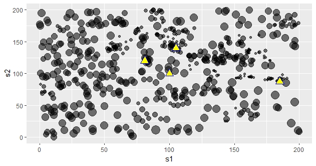
We illustrate the above on a real dataset as suggested in Example 5.3 of Taddy and Kottas, 2012. The suggested dataset, longleaf is part of the R package spatstat (Baddeley and Turner, 2005) and a detailed space-time survival analysis based on this was developed in Rathbun and Cressie, 1994. The observations are locations of 584 pine trees in a square and the marks are diameters of the trees at breast height (only for trees having this diameter greater than 2 cm). A scatter plot of the data is given in Figure 4. One can clearly see that the distribution of trees is not uniform, i.e., mature (larger diameter) trees are more evenly distributed than younger (smaller diameter) trees, which appear in clusters. Hence, the goal is to model the joint intensity of the locations and marks of these trees. Taddy and Kottas, 2012 model as a mixture model with a trivariate normal kernel and a mixing distribution defined over all the parameters of this multivariate normal distribution, i.e,
| (6) |
With the model in (6), we can estimate the conditional distribution of the marks at different locations to capture the varying distribution of trees, which in essence is an indication of the survival. We propose using the PR approach to fit this joint intensity function and estimate . Of course, that this is a mixture of a nine-dimensional latent variable space—three mean parameters and six covariance matrix parameters—makes it impossible to fit with the PR algorithm directly, so the PRticle filter approximation is necessary. Assuming a mixing distribution over all nine dimensions is possible using the PRticle filter approximation, but for model comparison we actually fit two models: the nine-dimensional model above and a reduced model that assumes the covariance terms in are fixed at 0. The mixing distribution is then estimated by PR with the PRticle filter approximation. From this fitted mixture model we extract the conditional density at specific locations to see how the diameter distribution varies with as displayed in Figure 5. As we can see in the scatter plot, each chosen location has unique characteristics in terms of diameter distribution. Locations and have higher concentrations of mature, large-diameter trees, which is correctly captured by both models (nine-dimensional and six-dimensional) in Figure 5. On the other hand, locations and have clusters of younger, smaller-diameter trees which, again, is correctly captured in Figure 5. Each plot in Figure 5 is overlaid with an empirical probability density of marks using the density function in R based on observations that are within a radius of 30 units from the chosen location. The fitted model retains these local features while being globally smoother than the empirical density. In terms of model comparison, both the six and nine-dimensional model reasonably capture the varying diameter distribution at all locations. A difference between the two estimates is that the full model estimate is smoother than the reduced model one. This is because the kernel density in the former inherently contains an average over the covariance parameters, while the latter fixes these at zero. The full model also appears to capture certain features better than the reduced model. For example, consider the locations and , whose conditional mark density is shown in Panels (c) and (d) of Figure 5, respectively. These two points have relatively high concentration of small-diameter trees, as seen in Figure 4; but upon closer inspection, the concentration at seems higher than at , and we see that the conditional density estimates based on the full model capture these differing features better than those based on the reduced mode. Similar results were obtained in Taddy and Kottas, 2012 via their proposed Dirichlet process mixture fit. An interesting difference between our results and those of Taddy and Kottas is that their plot at shows a sharp spike in the conditional density near , whereas ours does not. Since there is no evidence in the scatter plot for a high concentration of small-diameter trees, our guess is that their spike is actually a boundary effect, commonly seen in density estimation on bounded domains, and not an inherent feature in the data. That the PR estimate does not suffer from a boundary effect in this case is another benefit.
5 Conclusion
In this paper we proposed a new filtering mechanism, a PRticle filter, for fitting nonparametric mixture models using the PR algorithm in multivariate problems. This new development is an important addition because, previously, the PR algorithm could only handle mixtures over relatively low-dimensional spaces. This contribution creates new opportunities for PR-based methodology in non-trivial problems like marked spatial point process modelling in Section 4.2. Theoretically, we show that the PRticle filter approximation of the mixing distribution converges to the PR estimate in a strong sense as the number of particles goes to infinity, when the data of size remains fixed. This holds for the primary PR run only, an analysis of the attrition-handling embellishments in Section 3.3 would require more sophisticated techniques. Coupling this with results in literature on consistency (as ) of the PR estimator strengthens both the theoretical and practical aspects of PR. Our numerical results show that the PRticle filter approximation gives as accurate results as the traditional PR approach for univariate and bivariate mixtures and is also effective in estimating a multivariate mixture density.
One might also be interested in quantifying uncertainty about the mixing distribution and its features, like in Section 4.2. Capturing the variability in the PR estimate is a difficult problem, but suggestions have been made in Fortini and Petrone, 2020 and Dixit and Martin, 2019. The former uses a quasi-Bayes strategy to construct credible intervals for the PR estimate, while in the latter we leverage the order dependence of the PR estimator for uncertainty quantification. This strategy, which constructs multiple PR estimates based on distinct permutation of the data sequence, would be applicable for the PRticle filter approximation. There are some theoretical gaps that need to be filled, however, so remains an ongoing work.
One of our numerical illustrations considered nonparametric estimation of mixing distributions supported on the sphere in three-dimensions. A natural question is if this approach could be extended to other cases involving mixture defined on more general compact manifolds, e.g., higher-dimensional spheres, tori, etc. All that would be needed to extend the proposed strategy in such cases is a map from the surface of the manifold to an underlying Euclidean space where the comptutations can be carried out. In the special case of the sphere, there is a “global” Euclidean-space representation but, for more general manifolds, the corresponding Euclidean spaces would be “local,” which creates some new and interesting conceptual and computational challenges.
An interesting theoretical question is if consistency of the PRticle filter approximation could be established. That is, if is the PRticle filter approximation of the PR estimator , then the goal would be to show that as both and go to infinity. Of course, this would require to be increasing sufficiently fast with . Direct extension of the argument used in the proof of Theorem 1 may be possible using some naive techniques, e.g., the classical union bound, but, if successful, this would require to be exponentially large with . Our gut feeling is that such a large number of particles would not be necessary, so some important insights are still missing. We save this as a topic for future work.
A remaining practical challenge is the handling of attrition when the dimension of the mixing distribution support is relatively high. What we proposed in Section 3.3 is able to adequately control attrition rates for mixtures over at least nine-dimensional spaces. We have not thoroughly tested the performance of the PRticle filter approximation in dimensions higher than this, but we fully expect that controlling the attrition rate will be more and more difficult as the dimension increases. This is not a limitation of the proposed method, it is a challenge that any importance sampling-based method will face in high-dimensional applications. New insights would be needed to make this leap to high-dimensional mixtures but it may be possible to take advantage of the PR-specific recursive structure that we used to develop the PRticle filter approximation here.
Acknowledgments
The authors thank the three anonymous reviewers for their helpful feedback on an earlier version of this manuscript. This work was supported by the U.S. National Science Foundation, grant DMS–1737929.
Appendix A Proof of Theorem 1
Recall that,
where and
By the strong law of large numbers, we have that
To prove a similar claim for all , we proceed by induction. That is, we start by assuming that
| (7) |
and then use that assumption, along with the structure of the algorithm, to prove
Towards this, we have
The product above can be expanded as
where is a generic subset of and the sums and products are over all such subsets. Going back the formula for , we can distribute the average over through the product, which gives
By the induction hypothesis (7), we have that
Moreover, by the assumption (4), the strong law of large numbers gives
with -probability 1, as , again uniformly in . The two “uniformly in ” claims above follow because there are only finitely many such . Putting everything together, we have that converges with -probability 1, as , to
Moving the integration over to the outside of the sum over and undoing the product expansion above eventually leads to with -probability 1.
We showed above that
uniformly in without any assumptions on the convergence of the mixing distribution approximation. Since the final mixing density estimator is a continuous function of , it follows that
Since these are density functions, it follows from Scheffé’s theorem that converges in to , with -probability 1, as .
References
- Agapiou et al., (2017) Agapiou, S., Papaspiliopoulos, O., Sanz-Alonso, D., and Stuart, A. (2017). Importance sampling: Intrinsic dimension and computational cost. Statistical Science, 32(3):405–431.
- Baddeley and Turner, (2005) Baddeley, A. and Turner, R. (2005). spatstat: An R package for analyzing spatial point patterns. Journal of Statistical Software, 12(6):1–42.
- Blackwell and MacQueen, (1973) Blackwell, D. and MacQueen, J. B. (1973). Ferguson distributions via Pólya urn schemes. The Annals of Statistics, 1(2):353–355.
- Bugallo et al., (2017) Bugallo, M. F., Elvira, V., Martino, L., Luengo, D., Miguez, J., and Djuric, P. M. (2017). Adaptive importance sampling: The past, the present, and the future. IEEE Signal Processing Magazine, 34(4):60–79.
- (5) Carvalho, C. M., Johannes, M. S., Lopes, H. F., and Polson, N. G. (2010a). Particle learning and smoothing. Statistical Science, 25(1):88–106.
- (6) Carvalho, C. M., Lopes, H. F., Polson, N. G., and Taddy, M. A. (2010b). Particle learning for general mixtures. Bayesian Analysis, 5(4):709–740.
- DasGupta, (2008) DasGupta, A. (2008). Asymptotic Theory of Statistics and Probability. Springer Science & Business Media.
- Del Moral et al., (2006) Del Moral, P., Doucet, A., and Jasra, A. (2006). Sequential Monte Carlo samplers. Journal of the Royal Statistical Society: Series B (Statistical Methodology), 68(3):411–436.
- Dixit and Martin, (2019) Dixit, V. and Martin, R. (2019). Permutation-based uncertainty quantification about a mixing distribution. arXiv preprint arXiv:1906.05349.
- Dixit and Martin, (2021) Dixit, V. and Martin, R. (2021). Revisiting consistency of a recursive estimator of mixing distributions. arXiv preprint arXiv:2110.02465.
- Dixit and Martin, (2022) Dixit, V. and Martin, R. (2022). Estimating a mixing distribution on the sphere using predictive recursion. Sankhya B, 84:596–626.
- Doucet et al., (2001) Doucet, A., De Freitas, N., and Gordon, N. J. (2001). Sequential Monte Carlo Methods in Practice. Springer.
- Doucet and Johansen, (2011) Doucet, A. and Johansen, A. M. (2011). A tutorial on particle filtering and smoothing: Fiteen years later. In The Oxford Handbook of Nonlinear Filtering, pages 656–705. Oxford University Press.
- Fan, (1991) Fan, J. (1991). On the optimal rates of convergence for nonparametric deconvolution problems. The Annals of Statistics, 19(3):1257–1272.
- Ferguson, (1974) Ferguson, T. S. (1974). Prior distributions on spaces of probability measures. The Annals of Statistics, 2(4):615–629.
- Fortini and Petrone, (2020) Fortini, S. and Petrone, S. (2020). Quasi-Bayes properties of a procedure for sequential learning in mixture models. Journal of the Royal Statistical Society: Series B (Statistical Methodology), 82(4):1087–1114.
- Ghosal and Van der Vaart, (2017) Ghosal, S. and Van der Vaart, A. (2017). Fundamentals of nonparametric Bayesian inference, volume 44. Cambridge University Press.
- Ghosh and Ramamoorthi, (2003) Ghosh, J. and Ramamoorthi, R. (2003). Bayesian Nonparametrics. Springer.
- Hjort et al., (2010) Hjort, N. L., Holmes, C., Müller, P., and Walker, S. G. (2010). Bayesian nonparametrics, volume 28. Cambridge University Press.
- Kong, (1992) Kong, A. (1992). A note on importance sampling using standardized weights. University of Chicago, Dept. of Statistics, Tech. Rep, 348.
- Kottas and Sansó, (2007) Kottas, A. and Sansó, B. (2007). Bayesian mixture modeling for spatial poisson process intensities, with applications to extreme value analysis. Journal of Statistical Planning and Inference, 137(10):3151–3163.
- Liang et al., (2008) Liang, S., Carlin, B. P., and Gelfand, A. E. (2008). Analysis of Minnesota colon and rectum cancer point patterns with spatial and nonspatial covariate information. The Annals of Applied Statistics, 3(3):943–962.
- Lindsay, (1983) Lindsay, B. G. (1983). The geometry of mixture likelihoods: a general theory. The Annals of Statistics, 11(1):86–94.
- MacEachern et al., (1999) MacEachern, S. N., Clyde, M., and Liu, J. S. (1999). Sequential importance sampling for nonparametric Bayes models: The next generation. Canadian Journal of Statistics, 27(2):251–267.
- Martin, (2021) Martin, R. (2021). A survey of nonparametric mixing density estimation via the predictive recursion algorithm. Sankhya B, 83:97–121.
- Martin and Han, (2016) Martin, R. and Han, Z. (2016). A semiparametric scale-mixture regression model and predictive recursion maximum likelihood. Computational Statistics and Data Analysis, 94:75–85.
- Martin and Tokdar, (2009) Martin, R. and Tokdar, S. T. (2009). Asymptotic properties of predictive recursion: robustness and rate of convergence. Electronic Journal of Statistics, 3:1455–1472.
- Martin and Tokdar, (2011) Martin, R. and Tokdar, S. T. (2011). Semiparametric inference in mixture models with predictive recursion marginal likelihood. Biometrika, 98(3):567–582.
- Martin and Tokdar, (2012) Martin, R. and Tokdar, S. T. (2012). A nonparametric empirical Bayes framework for large-scale multiple testing. Biostatistics, 13(3):427–439.
- Newton, (2002) Newton, M. A. (2002). On a nonparametric recursive estimator of the mixing distribution. Sankhya A, 64(2):306–322.
- Newton et al., (1998) Newton, M. A., Quintana, F. A., and Zhang, Y. (1998). Nonparametric Bayes methods using predictive updating. In Practical Nonparametric and Semiparametric Bayesian Statistics, pages 45–61. Springer.
- Rathbun and Cressie, (1994) Rathbun, S. L. and Cressie, N. (1994). A space-time survival point process for a longleaf pine forest in southern Georgia. Journal of the American Statistical Association, 89(428):1164–1174.
- Ross and Markwick, (2019) Ross, G. J. and Markwick, D. (2019). dirichletprocess: An R package for fitting complex Bayesian nonparametric models. R package version 0.4.0.
- Stefanski and Carroll, (1990) Stefanski, L. and Carroll, R. J. (1990). Deconvoluting kernel density estimators. Statistics, 21(2):169–184.
- Taddy and Kottas, (2012) Taddy, M. A. and Kottas, A. (2012). Mixture modeling for marked poisson processes. Bayesian Analysis, 7(2):335–362.
- Tansey et al., (2018) Tansey, W., Koyejo, O., Poldrack, R. A., and Scott, J. G. (2018). False discovery rate smoothing. Journal of the American Statistical Association, 113(523):1156–1171.
- Tokdar and Kass, (2010) Tokdar, S. T. and Kass, R. E. (2010). Importance sampling: a review. Wiley Interdisciplinary Reviews: Computational Statistics, 2(1):54–60.
- Tokdar et al., (2009) Tokdar, S. T., Martin, R., and Ghosh, J. K. (2009). Consistency of a recursive estimate of mixing distributions. The Annals of Statistics, 37(5A):2502–2522.
- Tyler, (1987) Tyler, D. E. (1987). Statistical analysis for the angular central Gaussian distribution on the sphere. Biometrika, 74(3):579–589.
- Woody et al., (2022) Woody, S., Padilla, O. H. M., and Scott, J. G. (2022). Optimal post-selection inference for sparse signals: a nonparametric empirical Bayes approach. Biometrika, 109(1):1–16.