A Variational Approach For Price Formation Models In One DimensionThanks: King Abdullah University of Science and Technology (KAUST), CEMSE Division, Thuwal 23955-6900. Saudi Arabia. e-mail: yuri.ashrafyan@kaust.edu.saThanks: King Abdullah University of Science and Technology (KAUST), CEMSE Division, Thuwal 23955-6900. Saudi Arabia. e-mail: tigran.bakaryan@kaust.edu.saThanks: King Abdullah University of Science and Technology (KAUST), CEMSE Division, Thuwal 23955-6900. Saudi Arabia. e-mail: diogo.gomes@kaust.edu.saThanks: King Abdullah University of Science and Technology (KAUST), CEMSE Division, Thuwal 23955-6900. Saudi Arabia. e-mail: julian.gutierrezpineda@kaust.edu.saThanks: The authors were partially supported by King Abdullah University of Science and Technology (KAUST) baseline funds and KAUST OSR-CRG2021-4674.

Yuri Ashrafyan , Tigran Bakaryan , Diogo Gomes and Julian Gutierrez

Date: August 11, 2026

Abstract.

In this paper, we study a class of first-order mean-field games (MFGs) that model price formation. Using Poincaré Lemma, we eliminate one of the equations and obtain a variational problem for a single function. This variational problem offers an alternative approach for the numerical solution of the original MFGs system. We show a correspondence between solutions of the MFGs system and the variational problem. Moreover, we address the existence of solutions for the variational problem using the direct method in the calculus of variations. We end the paper with numerical results for a linear-quadratic model.

Key words and phrases:

Mean Field Games; Price formation; Potential Function, Lagrange multiplier

1. Introduction

Here, we consider the numerical solution of the first-order mean-field games (MFGs) system introduced in [31] to model price formation. The solution to this system determines the price $\varpi$ of a commodity with supply $Q$ when a large group of rational agents trades that commodity. The original price problem reads as follows:

Problem 1.

Suppose that $m_{0}\in\mathcal{P}({\mathbb{R}})$ , $H\in C^{1}({\mathbb{R}})$ , and $Q$ , $V$ , and $u_{T}$ are continuous. Assume further that $H$ is uniformly convex. Find $u,m:[0,T]\times{\mathbb{R}}\to{\mathbb{R}}$ and $\varpi:[0,T]\to{\mathbb{R}}$ satisfying $m\geqslant 0$ ,

(1.1)

\begin{cases}-u_{t}+H(\varpi+u_{x})+V(x)=0&[0,T]\times{\mathbb{R}},\\ m_{t}-\left(H^{\prime}(\varpi+u_{x})m\right)_{x}=0&[0,T]\times{\mathbb{R}},\\ -\int_{{\mathbb{R}}}H^{\prime}(\varpi+u_{x})m{\rm d}x=Q(t)&[0,T],\end{cases}

and

(1.2)

\begin{cases}m(0,x)=m_{0}(x)&\\ u(T,x)=u_{T}(x)&\end{cases}x\in{\mathbb{R}}.

The existence of solutions $(u,m,\varpi)$ to the previous problem was proved in [31]. The first equation is solved in the viscosity sense by the value function of a typical player $u\in C([0,T]\times{\mathbb{R}})$ . The second equation is solved in the distributional sense by the probability distribution of the agents, $m\in C([0,T],{\mathcal{P}}({\mathbb{R}}))$ . The price $\varpi$ is a continuous function on $[0,T]$ .

Price formation models offer a load-adaptive pricing strategy relevant in energy markets. For instance, [6] and [7] modeled intraday electricity markets, obtaining a price from the solution of forward-backward equations. In [24] and [28] authors studied the effects of a major player in the market. The latest paper considered $N$ -agent setting. A deterministic $N$ -agent price model was studied in [8]. A MFG model of homogeneous agents for the electricity markets was considered in [25]. In [4], the price equilibrium is obtained for a finite number of agents who optimally control their production and trading rates in order to satisfy a demand subjected to common noise. Stackelberg games for price formation under revenue optimization were proposed in [13] and [40], and Cournot models in [21]. A MFG of optimal switching was presented in [5] to model the transition to renewable energies. Other works incorporating market-clearing conditions are [41] and [27], the former specialized to Solar Renewable Energy Certificate Markets and the latter in exchange markets. The stochastic supply case was studied in [29], where authors obtained a price from a Lagrange multiplier rule for the balance constraint.

The standard MFG system exhibits a coupling of two partial differential equations with initial and terminal conditions (see for example [16]). Several numerical methods have been proposed to solve these MFG systems. Finite differences schemes and Newton-based methods were introduced in [1] and [2]. A recent survey can be found in [3]. Optimization methods and Fourier series approximations were proposed in [35]. Machine learning methods have been studied in [17], [18], [39], and [34]. However, the MFG system (1.1)-(1.2) not only couples a forward equation for $m$ with a backward equation for $u$ but also determines the coupling term $\varpi$ through an integral constraint, which is the third equation in (1.1). Therefore, the numerical approximation of the solution $(u,m,\varpi)$ of Problem 1 is challenging, and the main application of our methods is a novel numerical scheme for Problem 1.

The word Potential in MFGs is used in two unrelated contexts. Potential MFGs ([33], [16], [36]) are MFG systems given by the first-order optimality conditions of a minimization problem. Previously, standard optimization techniques were used for its numerical solution ([14]). In contrast, our potential approach relies on the structure of the continuity equation and Poincaré lemma ([19], Theorem 1.22). We introduce a potential functional that integrates the transport equation in (1.1).

Poincaré lemma was used for the continuity equation in [12] for the MFG planning problem. The authors obtained a variational problem for a potential function by eliminating one of the equations in the MFG system. Moreover, the solution $(u,m)$ of the planning MFG can be recovered using only the solution of the variational problem. The structure of the MFG planning problem differs from that in Problem 1 in two critical aspects: the initial-terminal conditions and the way the constraint couples the equations.

In Section 2, we use the existence result for Problem 1 provided in [31] to formally obtain a potential function, $\varphi$ . We show that (1.1) corresponds to the Euler-Lagrange equation of a constrained variational problem depending on $\varphi$ . To introduce this problem, let $F$ be the Legendre transform of $H$ ; that is,

(1.3)

F(y)=\sup_{p\in{\mathbb{R}}}\left[py-H(p)\right],\quad y\in{\mathbb{R}},

and let $L:{\mathbb{R}}\times{\mathbb{R}}_{0}^{+}\to{\mathbb{R}}_{0}^{+}$ be given by

(1.4)

L(z,y)=\begin{cases}F\left(\frac{z}{y}\right)y,&(z,y)\in{\mathbb{R}}\times{\mathbb{R}}^{+},\\ +\infty,&z\neq 0,\,y=0,\\ 0,&z=0,\,y=0.\end{cases}

The constrained variational problem is

Problem 2.

Suppose that $m_{0}\in\mathcal{P}({\mathbb{R}})$ , $H$ is uniformly convex, and $Q$ , $V$ , and $u_{T}$ are continuous. Find $\varphi:[0,T]\times{\mathbb{R}}\to{\mathbb{R}}$ that minimizes the functional

\varphi\mapsto\int_{0}^{T}\int_{{\mathbb{R}}}L(\varphi_{t},\varphi_{x})-V(x)\varphi_{x}-u^{\prime}_{T}(x)\varphi_{t}~{\rm d}x{\rm d}t,

over the set of functions such that $\varphi_{x}(t,\cdot)$ is a probability density on ${\mathbb{R}}$ for $t\in[0,T]$ , $\varphi_{x}(0,\cdot)=m_{0}(\cdot)$ , and satisfying

(1.5)

\int_{{\mathbb{R}}}\varphi(t,x)-M_{0}(x){\rm d}x=-\int_{0}^{t}Q(s){\rm d}s,\quad t\in[0,T].

We work under assumptions similar to those in [31] used to prove the existence and uniqueness of solutions to Problem 1. The precise statement of our assumptions is presented in Section 3. We rigorously study Problem 2 in Section 4, where we show that its formulation is independent of the solution $(u,m,\varpi)$ of Problem 1, and relies only on problem data. In Section 5, we obtain the existence of a price $\varpi$ in (1.1) as a Lagrange multiplier, and we establish the following connection between solutions of Problems 1 and 2:

Theorem 1.1.

Suppose that $\varphi\in C^{2}([0,T]\times{\mathbb{R}})$ solves Problem 2 . Then, the solution $(u,m,\varpi)$ of Problem 1 admits the representation

\displaystyle\begin{cases}u(t,x)=u_{T}(x)-\int_{t}^{T}H\left(F^{\prime}\left(\frac{\varphi_{t}(s,x)}{\varphi_{x}(s,x)}\right)\right){\rm d}s-(T-t)V(x),\quad&(t,x)\in[0,T]\times{\mathbb{R}}\\ m(t,x)=\varphi_{x}(t,x),\quad&(t,x)\in[0,T]\times{\mathbb{R}}\\ \varpi(t)=w_{T}-\int_{t}^{T}w(s){\rm d}s,\quad&t\in[0,T],\end{cases}

where $w_{T}=\int_{{\mathbb{R}}}(L^{*}_{z}(T,y)-u^{\prime}_{T}(y))\varphi_{x}(T,y){\rm d}y$ ,

w(s)=\int_{{\mathbb{R}}}\bigg(\left(L^{*}_{z}(s,y)\right)_{t}+\left(L^{*}_{y}(s,y)-V(y)\right)_{x}\bigg)\varphi_{x}(s,y){\rm d}y,\quad s\in[0,T],

and $L^{*}_{z}$ and $L^{*}_{y}$ are defined in (5.10) and (5.11), respectively.

Because Problem 2 is a convex minimization problem, we approximate its solution $\varphi$ by using standard optimization methods. Furthermore, using the approximations for $\varphi$ and Theorem 1.1, we obtain efficient approximation methods for the solution to Problem 1. In Section 6, we illustrate the implementation of our approach for the linear-quadratic setting, for which explicit formulas are provided in [31] that can be used as benchmarks. For all these benchmarks, our numerical method provides accurate approximations.

2. Derivation of the variational problem

In this section, we present a formal derivation of the variational problem for the potential function using the solution of the MFGs system. The precise assumptions we work with are stated in Section 3. The rigorous statement of the variational problem is given in Section 4, where we no longer rely on the solution of the MFGs system.

Let $(u,m,\varpi)$ solve Problem 1 with $m>0$ . Then, the second equation in (1.1) can be written as

\text{div}_{(t,x)}\left(m,-H^{\prime}(\varpi+u_{x})m\right)=0,\quad[0,T]\times{\mathbb{R}}.

The previous equation combined with Poincaré lemma (see [19], Theorem 1.22) gives the existence of a function (the potential) $\varphi:[0,T]\times{\mathbb{R}}\to{\mathbb{R}}$ such that

(2.1)

\begin{cases}m=\varphi_{x},\\ H^{\prime}(\varpi+u_{x})m=\varphi_{t}.\end{cases}

Because $H$ is uniformly convex, $H^{\prime}$ is strictly monotone. Therefore, by (1.3), we have

(2.2)

F^{\prime}(y)=\left(H^{\prime}\right)^{-1}(y).

Hence, from the second equation in (2.1), we deduce that

u_{x}=F^{\prime}\left(\frac{\varphi_{t}}{\varphi_{x}}\right)-\varpi.

If $V\in C^{1}({\mathbb{R}})$ , and $u$ is twice differentiable, we differentiate the Hamilton-Jacobi equation in (1.1) with respect to $x$ to obtain

-(u_{x})_{t}+\left(H(\varpi+u_{x})\right)_{x}+V^{\prime}=0.

Thus, the system (1.1) in terms of $\varphi$ is reduced to the following two equations

(2.3)

\begin{cases}-\left(F^{\prime}\left(\frac{\varphi_{t}}{\varphi_{x}}\right)-\varpi\right)_{t}+\left(H\left(F^{\prime}\left(\frac{\varphi_{t}}{\varphi_{x}}\right)\right)\right)_{x}+V^{\prime}=0&[0,T]\times{\mathbb{R}},\\ -\int_{{\mathbb{R}}}\varphi_{t}+Q\varphi_{x}~{\rm d}x=0&t\in[0,T],\end{cases}

with initial condition, $\varphi(0,x)=\int_{-\infty}^{x}m_{0}(y){\rm d}y\,\ x\in{\mathbb{R}}$ , and terminal condition

(2.4)

F^{\prime}\left(\frac{\varphi_{t}(T,x)}{\varphi_{x}(T,x)}\right)-\varpi(T)=u^{\prime}_{T}(x)\quad x\in{\mathbb{R}}.

Remark 2.1.

Notice that the initial condition implies that $\varphi_{x}(0,x)=m_{0}(x)$ , $x\in{\mathbb{R}}$ , which is the first equation in (1.2). Moreover, we have the following explicit formula for $\varphi$ in terms of the solution $(u,m,\varpi)$ of (1.1) and (1.2)

(2.5)

\varphi(t,x)=\int_{-\infty}^{x}m_{0}(y){\rm d}y+\int_{0}^{t}H^{\prime}(\varpi(s)+u_{x}(s,x))m(s,x){\rm d}s,\quad(t,x)\in[0,T]\times{\mathbb{R}}.

Therefore, the potential function $\varphi$ , which in principle has a closed formula arising from the solution of (1.1) and (1.2), can be characterized using the initial condition with $m_{0}$ , (2.3) and (2.4), which depend only, up to $\varpi$ , on problem data.

Remark 2.2.

Notice that the first equation in (2.3) shows that the expression

-\left(F^{\prime}\left(\frac{\varphi_{t}}{\varphi_{x}}\right)\right)_{t}+\left(H\left(F^{\prime}\left(\frac{\varphi_{t}}{\varphi_{x}}\right)\right)\right)_{x}+V^{\prime}

is independent of $x\in{\mathbb{R}}$ , so it is a function of time only and equal to $\dot{\varpi}$ . Similarly, (2.4) shows that

F^{\prime}\left(\frac{\varphi_{t}(T,x)}{\varphi_{x}(T,x)}\right)-u^{\prime}_{T}(x)

is independent of $x\in{\mathbb{R}}$ , and equal to the constant $\varpi(T)$ . Because any numerical method to compute $\varphi$ provides an approximation of the value $\varphi(t,x)$ , we can not expect the numerical approximation to be independent of $x$ in (2.3) and (2.4). Therefore, we can not rely on these formulas to recover $\varpi$ using an approximation of $\varphi$ . In Section 5, we provide a formula approximating $\varpi$ that averages the dependence on $x$ , and thus, can be implemented with any approximation of the potential.

Next, consider the functional

(2.6)

\begin{split}\int_{0}^{T}\int_{{\mathbb{R}}}L(\varphi_{t},\varphi_{x})-V\varphi_{x}{\rm d}x{\rm d}t-\int_{{\mathbb{R}}}u^{\prime}_{T}(x)(\varphi(T,x)-\varphi(0,x))~{\rm d}x\end{split}

subject to $\int_{{\mathbb{R}}}-(\varphi_{t}+Q\varphi_{x}){\rm d}x=0$ on $[0,T]$ , and with initial condition $\varphi(0,x)=\int_{-\infty}^{x}m_{0}(y){\rm d}y$ . Using the augmented functional associated with the constraint $\int_{{\mathbb{R}}}-(\varphi_{t}+Q\varphi_{x}){\rm d}x=0$ , we show that (2.3) is an Euler-Lagrange equation. Thus, we introduce a Lagrange multiplier $\varpi:[0,T]\to{\mathbb{R}}$ for the integral constraint, and we define

(2.7)

\begin{split}\tilde{I}[\varphi,\varpi]:=\int_{0}^{T}\int_{{\mathbb{R}}}L(\varphi_{t},\varphi_{x})-\varpi\left(\varphi_{t}+Q\varphi_{x}~\right)-V\varphi_{x}-u^{\prime}_{T}(x)\varphi_{t}~{\rm d}x{\rm d}t\end{split}

with initial condition $\varphi(0,x)=\int_{-\infty}^{x}m_{0}(y){\rm d}y$ . By considering critical points $(\varphi,\varpi)$ of the previous functional, we obtain that (2.3) is the corresponding Euler-Lagrange equation, with the natural boundary condition (2.4).

Proposition 2.3.

Let $(\varphi,\varpi)$ be a critical point of the functional (2.7) over $C^{2}([0,T]\times{\mathbb{R}})\times C^{1}([0,T])$ satisfying $\varphi(0,x)=\int_{-\infty}^{x}m_{0}(y){\rm d}y$ . Assume further that $\varphi_{x}>0$ . Then, the corresponding Euler-Lagrange equation is equivalent to (2.3)-(2.4).

Proof.

Let $(\varphi,\varpi)$ be a critical point of (2.7). Taking $(\beta^{1},\beta^{2})\in C^{1}_{c}((0,T]\times{\mathbb{R}})\times C([0,T])$ , we have

(2.8)

\left.\frac{d}{d\varepsilon}\tilde{I}[(\varphi,\varpi)+\varepsilon(\beta^{1},\beta^{2})]\right|_{\varepsilon=0}=0.

The previous identity implies that

(2.9)

-\left(L_{z}(\varphi_{t},\varphi_{x})-\varpi\right)_{t}-\left(L_{y}(\varphi_{t},\varphi_{x})\right)_{x}+V^{\prime}=0,

and

(2.10)

L_{z}(\varphi_{t}(T,x),\varphi_{x}(T,x))-\varpi(T)-u^{\prime}_{T}(x)=0

on $[0,T]\times{\mathbb{R}}$ . Because $\varphi_{x}>0$ , (1.4) gives

(2.11)

\begin{split}&L_{z}(\varphi_{t},\varphi_{x})=F^{\prime}\left(\frac{\varphi_{t}}{\varphi_{x}}\right),\\ &\left(L_{y}(\varphi_{t},\varphi_{x})\right)_{x}=\left(-\frac{\varphi_{t}}{\varphi_{x}}F^{\prime}\left(\frac{\varphi_{t}}{\varphi_{x}}\right)+F\left(\frac{\varphi_{t}}{\varphi_{x}}\right)\right)_{x}=-\frac{\varphi_{t}}{\varphi_{x}}\left(F^{\prime}\left(\frac{\varphi_{t}}{\varphi_{x}}\right)\right)_{x}.\end{split}

Notice that, by (2.2), we have

(2.12)

\left(H\left(F^{\prime}\left(\frac{\varphi_{t}}{\varphi_{x}}\right)\right)\right)_{x}=\frac{\varphi_{t}}{\varphi_{x}}\left(F^{\prime}\left(\frac{\varphi_{t}}{\varphi_{x}}\right)\right)_{x}.

Combining the identities in (2.11) with (2.12) and using (2.9), we deduce the first equation in (2.3). Using the first identity of (2.11) in (2.10), we obtain (2.4).

Finally, taking $\beta^{1}\equiv 0$ in (2.8), we obtain

\int_{0}^{T}\left(\int_{{\mathbb{R}}}-(\varphi_{t}+Q\varphi_{x}){\rm d}x\right)\beta^{2}~{\rm d}t=0,

where $\beta^{2}$ is arbitrary. Thus, the continuity of the map $t\mapsto\int_{{\mathbb{R}}}-(\varphi_{t}+Q\varphi_{x}){\rm d}x$ implies the second equation in (2.3). ∎

In Section 5, we address the existence of the price $\varpi$ as a Lagrange multiplier associated with a minimizer of (2.6).

3. Assumptions

In this section, we state the assumptions to prove the existence of minimizers of the functional (2.6). This set of assumptions is similar to the ones introduced in [31] to guarantee the existence and uniqueness of $(u,m,\varpi)$ solving (1.1) and (1.2).

The following two assumptions require standard growth and convexity properties for $H$ .

Assumption 1.

There exist constants, $c>0$ and $p>1$ , such that the Legendre-Fenchel transform of $H$ , the function $F$ in (1.3), satisfies

F(v)\geqslant c|v|^{p}.

Assumption 2.

For all $x\in{\mathbb{R}}$ , the map $p\mapsto H(p)$ is uniformly convex; that is, there exists a constant $\kappa>0$ such that $H^{\prime\prime}(p)\geqslant\kappa$ for all $p\in{\mathbb{R}}$ . Moreover, there exists a positive constant, $C$ , such that $|H^{\prime\prime\prime}|\leqslant C$ .

For the supply, to simplify, we assume it is a smooth function of time.

Assumption 3.

The supply function, $Q$ , is $C^{\infty}([0,T])$ .

The following assumption is technical and was used in [31] to get bounds for the price.

Assumption 4.

The potential $V$ , the terminal cost $u_{T}$ , the initial density function $m_{0}$ are $C^{2}({\mathbb{R}})$ functions and $V$ , $u_{T}$ are globally Lipschitz. Furthermore, there exists a constant $C>0$ such that

|V^{\prime\prime}|\leqslant C,\quad|u_{T}^{\prime\prime}|\leqslant C,\quad|m_{0}^{\prime\prime}|\leqslant C.

The following condition guarantees the uniqueness of solutions of (1.1) and (1.2).

Assumption 5.

The potential $V$ and the terminal cost $u_{T}$ are convex.

Finally, because we are interested in problems where agent’s assets are bounded, we require the following assumption on $m_{0}$ . This assumption further simplifies some technical points in the presentation.

Assumption 6.

The initial density function $m_{0}$ has compact support; that is, there exists $R_{0}>0$ such that $\operatorname{supp}(m_{0})\subset[-R_{0},R_{0}]$ .

4. The variational approach

Here, we examine a variational problem associated with the MFG system (1.1)-(1.2) continuing the formal derivation in Section 2. This problem is obtained by minimizing the functional (2.6) in a suitable class of admissible functions. We study the existence and uniqueness of solutions to this variational problem. In Section 5, we establish a formula representing the solution to the MFG system (1.1)-(1.2), in terms of the solution to this variational problem.

First, we recall that, under Assumptions 1-5, Theorem 1 in [31] gives existence and uniqueness of solutions $(u,m,\varpi)$ to Problem 1, where $m\in\mathcal{P}({\mathbb{R}})\cap C([0,T]\times{\mathbb{R}})$ . Moreover, $u$ is a viscosity solution to the first equation in (1.1), Lipschitz continuous and semi-concave in $x$ , and $u_{x}$ , $u_{xx}$ , $m$ are bounded. Furthermore, by the results in [10], $\varpi$ is Lipschitz continuous.

4.1. Preliminary results for the continuity equation

Before we formulate our variational problem, we prove a general result for the continuity equation (the second equation in (1.1)) that motivates the choice of the function spaces. We recall the following result from [15] about the existence and uniqueness of solutions to the continuity equation. Let $\mu_{0}\in C^{1}({\mathbb{R}})$ , $b\in L^{1}([0,T];W_{loc}^{1,1}({\mathbb{R}}))\cap C([0,T]\times{\mathbb{R}})$ and $b_{x}\in L^{\infty}([0,T]\times{\mathbb{R}})$ . Then, the continuity equation

(4.1)

\begin{cases}\mu_{t}-(b\mu)_{x}=0&[0,T]\times{\mathbb{R}},\\ \mu(0,x)=\mu_{0}(x)&x\in{\mathbb{R}}\end{cases}

has a unique solution $\mu\in L^{\infty}([0,T]\times{\mathbb{R}})$ in distributional sense. The existence result follows from Theorem 1.1 in [15], which addresses the existence and uniqueness of distributional solutions to the continuity equation (4.1) for a vector field $b$ satisfying weaker conditions.

Now, we prove that if the initial condition $\mu_{0}$ of the continuity equation is compactly supported, the solution $\mu$ is also compactly supported.

Proposition 4.1.

Let $\mu_{0}\in C^{1}({\mathbb{R}})$ , $b\in L^{1}([0,T];W_{loc}^{1,1}({\mathbb{R}}))\cap C([0,T]\times{\mathbb{R}})$ and $b_{x}\in L^{\infty}([0,T]\times{\mathbb{R}})$ . Assume further that $\mu_{0}\in C_{c}^{1}({\mathbb{R}})$ . Then, the unique solution to the continuity equation (4.1) has compact support; that is, $\mu\in L_{c}^{\infty}([0,T]\times{\mathbb{R}})$ .

Proof.

From the results in [15], it follows that there exists a unique, $\mu\in L^{\infty}([0,T]\times{\mathbb{R}})$ solving (4.1) in the distributional sense. Let $b^{\varepsilon}$ be a sequence of functions in $C^{\infty}([0,T]\times{\mathbb{R}})$ satisfying:

•

$b^{\varepsilon}$ is Lipschitz continuous w.r.t. $x$ , and its Lipschitz constant satisfies $\mbox{Lip}(b^{\varepsilon})\leqslant\mbox{Lip}(b)$ ,
•

$b^{\varepsilon}\to b$ uniformly on every compact set of $[0,T]\times{\mathbb{R}}$ .

We can obtain such sequence $b^{\varepsilon}$ by considering the convolution with standard mollifiers in $x$ and a partition of unity construction in $t$ . Next, we consider the continuity equation with the vector field $b^{\varepsilon}$

(4.2)

\begin{cases}\mu^{\varepsilon}_{t}-(b^{\varepsilon}\mu^{\varepsilon})_{x}=0&[0,T]\times{\mathbb{R}},\\ \mu^{\varepsilon}(0,x)=\mu_{0}(x)&x\in{\mathbb{R}}.\end{cases}

Because $b^{\varepsilon},\,b_{x}^{\varepsilon}\in C^{1}([0,T]\times{\mathbb{R}})$ , by Theorem 6.3 in [38], (4.2) has a unique solution $\mu^{\varepsilon}\in C^{1}([0,T]\times{\mathbb{R}})$ given by

(4.3)

\mu^{\varepsilon}(t,X^{\varepsilon}(t;y))J(t;y)=\mu_{0}(y),\quad(t,y)\in[0,T]\times{\mathbb{R}},

where

(4.4)

J(t;y)=\exp\left(\int_{0}^{t}b^{\varepsilon}_{x}(s,X^{\varepsilon}(s;y))~{\rm d}s\right),

and $X^{\varepsilon}$ solves the following initial value problem

(4.5)

\begin{cases}\dot{X}^{\varepsilon}(t;y)=b^{\varepsilon}(t,X^{\varepsilon}(t;y))&\quad(t,y)\in(0,T]\times{\mathbb{R}},\\ X^{\varepsilon}(0;y)=y&\quad y\in{\mathbb{R}}.\end{cases}

Because $b^{\varepsilon}\in C^{1}([0,T]\times{\mathbb{R}})$ , the map $y\mapsto X^{\varepsilon}(t;y)$ is a diffeomorphism (see [37], Chapter 3). Moreover, because $b^{\varepsilon}\in C^{1}([0,T]\times{\mathbb{R}})$ is Lipschitz continuous w.r.t. $x$ , we have $|b^{\varepsilon}(t,x)|\leqslant C_{\varepsilon}\left(1+|x|\right)$ , where, by the uniform convergence of $b^{\varepsilon}$ to $b$ on compact sets,

(4.6)

C_{\varepsilon}\leqslant\max\{1+|b(t,0)|,\mbox{Lip}(b)\}.

Applying Grönwall’s inequality to (4.5), provides

(4.7)

|X^{\varepsilon}(t;y)|\leqslant\left(|y|+C_{\varepsilon}T\right)\left(1+C_{\varepsilon}Te^{C_{\varepsilon}T}\right).

Because $|y|>R_{0}$ implies $\mu_{0}(y)=0$ for some $R_{0}>0$ , (4.3) shows that $\mu^{\varepsilon}$ may have non-zero values only for those $y$ satisfying $|y|\leqslant R_{0}$ , for which (4.7) implies

|X^{\varepsilon}(t;y)|\leqslant\left(R_{0}+C_{\varepsilon}T\right)\left(1+C_{\varepsilon}Te^{C_{\varepsilon}T}\right)=:R_{\varepsilon}.

Thus, $\mbox{supp}(\mu^{\varepsilon})\subset[0,T]\times[-R_{\varepsilon},R_{\varepsilon}]$ , which, by (4.6), provides the existence of $R>0$ , depending on $T$ and $\mbox{Lip}(b)$ , such that $\operatorname{supp}\mu^{\varepsilon}\subset[-R,R]$ for every $1\gg\varepsilon>0$ . Furthermore, (4.3) and (4.4) imply that there exists $C\geqslant 0$ , depending on $T$ , $\mbox{Lip}(b)$ and $\mu_{0}$ , such that $||\mu^{\varepsilon}||_{L^{\infty}([0,T]\times{\mathbb{R}})}\leqslant C$ for all $1\gg\varepsilon>0$ . Hence, by Banach-Alaoglu theorem, there exists $\bar{\mu}\in L^{\infty}([0,T]\times{\mathbb{R}})$ such that

\mu^{\varepsilon}\overset{\ast}{\rightharpoonup}\bar{\mu}\quad\mbox{as}\quad\varepsilon\to 0\quad\text{in}\quad L^{\infty}([0,T]\times{\mathbb{R}}).

Consequently, $\operatorname{supp}\bar{\mu}\subset[-R,R]$ as well. On the other hand, $\mu^{\varepsilon}$ also solves (4.2) in the sense of distributions; that is,

(4.8)

-\int_{0}^{T}\int_{{\mathbb{R}}}\mu^{\varepsilon}\left(\phi_{t}-b^{\varepsilon}\phi_{x}\right){\rm d}x{\rm d}t=\int_{{\mathbb{R}}}\mu_{0}\phi~{\rm d}x,

for any $\phi\in C^{1}_{c}([0,T)\times{\mathbb{R}})$ .

Thus, given $\phi\in C^{1}_{c}([0,T)\times{\mathbb{R}})$ , we write

(4.9)

\begin{split}&-\int_{0}^{T}\int_{{\mathbb{R}}}\bar{\mu}\left(\phi_{t}-b\phi_{x}\right){\rm d}x{\rm d}t\\ &=-\int_{0}^{T}\int_{{\mathbb{R}}}\mu^{\varepsilon}\left(\phi_{t}-b^{\varepsilon}\phi_{x}\right)+\left(\mu^{\varepsilon}-\bar{\mu}\right)\left(\phi_{t}-b\phi_{x}\right)+\mu^{\varepsilon}\phi_{x}\left(b-b^{\varepsilon}\right){\rm d}x{\rm d}t.\end{split}

Because $\phi_{t}$ , $\phi_{x}$ , $b\phi_{x}\in L^{1}([0,T]\times{\mathbb{R}})$ , the second term on the right-hand side of (4.9) vanishes as $\varepsilon\to 0$ . Furthermore, using the uniform bound for $\mu^{\varepsilon}$ , and because $b^{\varepsilon}$ converges uniformly to $b$ in the compact support of $\phi$ , we obtain that the third term on the right-hand side of (4.9) also vanishes as $\varepsilon\to 0$ . Thus, using (4.8), we get

-\int_{0}^{T}\int_{{\mathbb{R}}}\bar{\mu}\left(\phi_{t}-b\phi_{x}\right){\rm d}x{\rm d}t=\int_{{\mathbb{R}}}\mu_{0}\phi~{\rm d}x,

and since $\phi$ is arbitrary, we conclude that $\bar{\mu}$ is a solution to (4.1) in the distributional sense.

To conclude the proof, it is enough to recall that the results in [15] provide uniqueness for the initial value problem in (4.1), in the sense of the distributions. ∎

Applying the previous result to the MFG system (1.1)-(1.2), we obtain the following.

Corollary 4.2.

Suppose that Assumptions 1-5 hold. Let $(u,m,\varpi)$ be the solution to (1.1). Assume further that Assumption 6 holds with $R_{0}>0$ . Then, $m$ is compactly supported; that is, there exists a constant $R_{m}\geqslant R_{0}$ , such that $\operatorname{supp}m(t,\cdot)\subseteq[-R_{m},R_{m}]$ for $t\in[0,T]$ . Moreover, $R_{m}$ is bounded by a constant that depends only on the problem data.

Proof.

Let $b(t,x)=H^{\prime}(\varpi(t)+u_{x}(t,x))$ denote the vector field of the continuity equation in (1.1). By Proposition 8 in [31], $|u_{xx}|\leqslant C(T,V,u_{T})$ , which implies that $u_{x}$ is Lipschitz w.r.t. $x$ . By Assumptions 1 and 2, for $p>2$ , $|H^{\prime\prime}|\leqslant C(F)$ , for some $C(F)>0$ . Thus, $b(t,\cdot)\in C^{1}({\mathbb{R}})$ is Lipschitz continuous in ${\mathbb{R}}$ uniformly with respect to $t$ . Furthermore, the Lipchitz constant satisfies

\mbox{Lip}(b(t,\cdot))\leqslant C_{0},

where $C_{0}=C_{0}(T,V,F,u_{T})$ . Therefore, Proposition 4.1 implies the first part of the result. Moreover, (4.7) shows that

(4.10)

R_{m}\leqslant\left(R_{0}+C_{0}T\right)\left(1+C_{0}Te^{C_{0}T}\right),

which concludes the proof. ∎

Remark 4.3.

Consider the potential $\varphi$ associated with the solution $(u,m,\varpi)$ of the MFG system (1.1)-(1.2), as given by (2.1). By Corollary 4.2, we deduce that the gradient of the potential $\varphi$ has compact support; that is, $\operatorname{supp}(\varphi_{t}(t,\cdot)),\operatorname{supp}(\varphi_{x}(t,\cdot))\subseteq[-R_{m},R_{m}]$ for all $t\in[0,T]$ . Thus, (4.10) shows that, by selecting

R>\left(R_{0}+C_{0}T\right)\left(1+C_{0}Te^{C_{0}T}\right),

we obtain a compact set $[-R,R]$ that depends only on problem data, and which contains the support of the gradient of $\varphi$ when (2.5) holds. Thus, using this compact set, we can formulate our variational problem independently of the solution $(u,m,\varpi)$ of the MFGs system (1.1) and (1.2). Notice that (2.5) already suggests a candidate for a minimizer. However, we study the existence of solutions to the variational problem independently of solutions to the MFGs system. Moreover, if uniqueness holds and we have existence for both problems, then (2.5) is the unique minimizer.

4.2. Statement of the variational problem

In this subsection, we present our variational approach rigorously using only problem data. We start with the notations and the definition of admissible functions. Then, we formulate and study the variational problem.

Let $R_{0}$ be given by Assumption 6 and let

(4.11)

R>\max\left\{\left(R_{0}+C_{0}T\right)\left(1+C_{0}Te^{C_{0}T}\right),R_{0}+\|Q\|_{L^{1}([0,T])}\right\}.

Notice that, by (4.10), $R$ is an upper bound for $R_{m}$ , as required, according to Remark 4.3. The additional requirement $R>R_{0}+\|Q\|_{L^{1}([0,T])}$ guarantees that the set of admissible functions that we define below is not empty. Set

\Omega_{R}=[0,T]\times[-R,R],\quad\Omega=[0,T]\times{\mathbb{R}}.

We denote by $\mathcal{M}(\Omega_{R})$ ( $\mathcal{M}(\Omega)$ ) the set of Radon measures on $\Omega_{R}\subset{\mathbb{R}}^{2}$ ( $\Omega\subset{\mathbb{R}}^{2}$ ) and by $BV(\Omega_{R})$ ( $BV(\Omega)$ ) the set of functions with bounded variation on $\Omega_{R}$ ( $\Omega$ ) (see [23], [9]).

To define the admissible set for our variational problem, we rewrite the balance condition, the second equation in (2.3). Recall that $\operatorname{supp}(m_{0})\subset[-R_{0},R_{0}]$ and $R>R_{0}$ . Let

(4.12)

M_{0}(x)=\int_{-\infty}^{x}m_{0}(y){\rm d}y=\int_{-R}^{x}m_{0}(y){\rm d}y,\quad x\in{\mathbb{R}},

be the cumulative density function of $m_{0}$ . Note that after integrating the balance condition over $[0,t]$ , and requiring that $\int_{{\mathbb{R}}}\varphi_{x}(t,x){\rm d}x=1$ for $t\in[0,T]$ (which follows in case that (2.1) holds), we get

\int_{0}^{t}\int_{{\mathbb{R}}}\varphi_{t}~{\rm d}x{\rm d}s=-\int_{0}^{t}Q(s){\rm d}s,\quad t\in[0,T].

Therefore, we write the balance condition as

(4.13)

\int_{{\mathbb{R}}}\varphi(t,x)-M_{0}(x)~{\rm d}x=-\int_{0}^{t}Q(s){\rm d}s,\quad t\in[0,T].

Relying on (4.13) and taking into account the discussion in Remark 4.3, for any set $A\subset{\mathbb{R}}^{2}$ satisfying $[0,T]\times[-R,R]\subseteq A$ , we denote

	$\displaystyle\mathcal{B}_{R}(A)=$	$\displaystyle\left\{(\varphi-M_{0})\in W^{1,1}(A):~\operatorname{supp}(\varphi_{t}(t,\cdot)),\operatorname{supp}(\varphi_{x}(t,\cdot))\subseteq(-R,R),~t\in[0,T]\right\},$
	$\displaystyle\mathcal{B}(A)=$	$\displaystyle\left\{\varphi\in\mathcal{B}_{R}(A):~\varphi_{x}\geqslant 0,~\varphi(0,x)=\int_{-R}^{x}m_{0}(y){\rm d}y,~x\in{\mathbb{R}}\right.$
		$\displaystyle\quad\left.\int_{{\mathbb{R}}}\varphi(t,x)-M_{0}(x)~{\rm d}x=-\int_{0}^{t}Q(s)~{\rm d}s,~\int_{-R}^{R}\varphi_{x}(t,x){\rm d}x=1,~t\in[0,T]\right\},$

which are convex sets. Before proceeding, we prove a crucial property of the set $\mathcal{B}(\Omega)$ .

Proposition 4.4.

For any function $\varphi\in\mathcal{B}(\Omega)$ , we have, for $t\in[0,T]$ ,

\varphi(t,x)=\begin{cases}0\quad&x\in(-\infty,-R],\\ \varphi(t,x)\quad&x\in(-R,R),\\ 1\quad&x\in[R,+\infty).\end{cases}

Proof.

Because $(\varphi-M_{0})\in W^{1,1}(\Omega)$ and $\lim\limits_{x\to+\infty}M_{0}(x)=1$ , for each $t\in[0,T]$ , there exists a sequence ${x_{k}}$ such that $x_{k}\to\infty$ and $\lim\limits_{k\to+\infty}\varphi(t,x_{k})=1$ . On the other hand, recalling that

\operatorname{supp}(\varphi_{t}(t,\cdot)),\operatorname{supp}(\varphi_{x}(t,\cdot))\subset(-R,R),

we have that $\varphi$ is constant on $\Omega\setminus[0,T]\times(-R,R)$ . Consequently, $\varphi(t,x)=1$ for $x\in[R,+\infty)$ . Similarly, we can prove that $\varphi(t,x)=0$ , $x\in(-\infty,-R]$ . ∎

Finally, the set of admissible functions for our variational problem is given by

(4.14)

\begin{split}\mathcal{A}(\Omega_{R})=\left\{\varphi\in\mathcal{B}(\Omega_{R}):~\varphi(t,-R)=0\right\}.\end{split}

As a result of Proposition 4.4, we obtain the following relation between the admissible set $\mathcal{A}(\Omega_{R})$ and the set $\mathcal{B}(\Omega)$ .

Corollary 4.5.

For any function $\varphi\in\mathcal{B}(\Omega)$ there exist a function $\tilde{\varphi}\in\mathcal{A}(\Omega_{R})$ such that $\varphi\equiv\tilde{\varphi}$ in $\Omega_{R}$ . The opposite is also true.

Under Assumption 4, we have

(4.15)

\left|\int_{\Omega_{R}}u^{\prime}_{T}(x)\varphi_{t}~{\rm d}x{\rm d}t\right|\leqslant\mbox{Lip}{(u_{T})}\int_{\Omega_{R}}|\varphi_{t}|~{\rm d}x{\rm d}t,

where $\mbox{Lip}{(u_{T})}$ is the Lipschitz constant of $u_{T}$ . Relying on the previous inequality, we consider the following variational problem

\begin{split}\inf_{\varphi\in\mathcal{B}(\Omega)}\int_{\Omega_{R}}L(\varphi_{t},\varphi_{x})-V\varphi_{x}-u^{\prime}_{T}(x)\varphi_{t}~{\rm d}x{\rm d}t,\end{split}

which, by Corollary 4.5, coincides with the following (see (2.6))

(4.16)

\inf_{\varphi\in\mathcal{A}(\Omega_{R})}I[\varphi],

where

I[\varphi]:=\int_{\Omega_{R}}L(\varphi_{t},\varphi_{x})-V\varphi_{x}-u^{\prime}_{T}(x)\varphi_{t}~{\rm d}x{\rm d}t.

As anticipated in Remark 4.3, (4.11) guarantees that the previous variational problem does not rely on the solution $(u,m,\varpi)$ to (1.1)-(1.2) but only on the data of Problem 1. Moreover, the infimum in (4.16) can be attained by at most one function, as we show next.

Proposition 4.6.

Suppose that Assumptions 1-6 hold. Then, at most, one function attains the infimum in (4.16).

Proof.

Let $\varphi^{1}$ and $\varphi^{2}$ attain the infimum in (4.16). By Proposition 4.7, we denote

\displaystyle\ell=\min\limits_{(\varphi)\in\mathcal{A}(\Omega_{R})}I[\varphi]\in{\mathbb{R}}.

Thus, $I[\varphi^{1}]=I[\varphi^{2}]=\mathcal{\ell}$ . Setting $\bar{\varphi}=\frac{1}{2}(\varphi^{1}+\varphi^{2})$ , and using the convexity of $L$ , we obtain

(4.17)

\ell\leqslant I[\bar{\varphi}]\leqslant\tfrac{1}{2}I[\varphi^{1}]+\tfrac{1}{2}I[\varphi^{2}]=\ell.

Hence, $\bar{\varphi}$ is also minimizer of (4.16). Let $\tilde{\varphi}=\frac{\varphi^{1}+\bar{\varphi}}{2}$ and

	$\displaystyle{\mathcal{U}}_{1}=\{(t,x)\in\Omega_{R}:{\varphi}_{x}^{1}>0\},\quad{\mathcal{U}}_{2}=\{(t,x)\in\Omega_{R}:{\varphi}_{x}^{2}>0\},$
	$\displaystyle\tilde{{\mathcal{U}}}=\{(t,x)\in\Omega_{R}:\tilde{\varphi}_{x}>0\}=\bar{{\mathcal{U}}}=\{(t,x)\in\Omega_{R}:\bar{\varphi}_{x}>0\}={\mathcal{U}}_{1}\cup{\mathcal{U}}_{2}.$

Arguing as in (4.17), we have

(4.18)

\ell\leqslant I[\tilde{\varphi}]\leqslant\tfrac{1}{2}I[\varphi^{1}]+\tfrac{1}{2}I[\bar{\varphi}]=\ell.

This with (4.17), yields that

\displaystyle L(\varphi^{1}_{t},\varphi^{1}_{x}),\,L(\varphi^{2}_{t},\varphi^{2}_{x}),\,L(\bar{\varphi}_{t},\bar{\varphi}_{x}),\,L(\tilde{\varphi}_{t},\tilde{\varphi}_{x})<+\infty\kern 5.0pt\hbox{a.e.~in }\Omega_{R}.

Therefore,

(4.19)			$\displaystyle\varphi^{1}_{t}=0\kern 5.0pt\text{ a.e.~in }\Omega_{R}\setminus{\mathcal{U}}_{1},$
			$\displaystyle\varphi^{2}_{t}=0\kern 5.0pt\text{ a.e.~in }\Omega_{R}\setminus{\mathcal{U}}_{2},$
			$\displaystyle\bar{\varphi}_{t}=0\kern 5.0pt\text{ a.e.~in }\Omega_{R}\setminus\bar{{\mathcal{U}}}$
			$\displaystyle\tilde{\varphi}_{t}=0\kern 5.0pt\text{ a.e.~in }\Omega_{R}\setminus\tilde{{\mathcal{U}}}.$

Furthermore, (4.18) implies

(4.20)

\begin{split}\int_{\Omega_{R}}\Big(\tfrac{1}{2}L(\varphi^{1}_{t},\varphi^{1}_{x})+&\tfrac{1}{2}L(\bar{\varphi}_{t},\bar{\varphi}_{x})-L(\tilde{\varphi}_{t},\tilde{\varphi}_{x})\Big)\,{\rm d}x{\rm d}t=0.\end{split}

The convexity of $L$ and (4.20) implies

\tfrac{1}{2}L(\varphi^{1}_{t},\varphi^{1}_{x})+\tfrac{1}{2}L(\bar{\varphi}_{t},\bar{\varphi}_{x})-L(\tilde{\varphi}_{t},\tilde{\varphi}_{x})=0,\quad\text{a.e. in }\Omega_{R}.

Consequently, the following also holds

(4.21)

\tfrac{1}{2}L(\varphi^{1}_{t},\varphi^{1}_{x})+\tfrac{1}{2}L(\bar{\varphi}_{t},\bar{\varphi}_{x})-L(\tilde{\varphi}_{t},\tilde{\varphi}_{x})=0,\quad\text{a.e. in }\quad{\mathcal{U}}_{1}\cap\bar{{\mathcal{U}}}\cap\tilde{{\mathcal{U}}}.

Because $L$ is strictly convex in ${\mathbb{R}}\times{\mathbb{R}}^{+}$ and ${\mathcal{U}}_{1}\cap\bar{{\mathcal{U}}}\cap\tilde{{\mathcal{U}}}={\mathcal{U}}_{1}\subset{\mathbb{R}}\times{\mathbb{R}}^{+}$ , we obtain from (4.21) that

\begin{cases}\varphi^{1}_{t}=\bar{\varphi}_{t}\\ \varphi^{1}_{x}=\bar{\varphi}_{x}.\end{cases}\quad\text{a.e. in}\quad{\mathcal{U}}_{1}

Hence,

(4.22)

\begin{cases}\varphi^{1}_{t}=\varphi^{2}_{t}\\ \varphi^{1}_{x}=\varphi^{2}_{x}.\end{cases}\quad\text{a.e. in}\quad{\mathcal{U}}_{1}

Taking $\varphi^{2}$ instead of $\varphi^{1}$ in (4.18) and arguing as before, we obtain

(4.23)

\begin{cases}\varphi^{1}_{t}=\varphi^{2}_{t}\\ \varphi^{1}_{x}=\varphi^{2}_{x}.\end{cases}\quad\text{a.e. in}\quad{\mathcal{U}}_{2}

Combing (4.19), (4.22) and (4.23), we conclude that $\varphi^{1}=\varphi^{2}$ . ∎

Next, we prove that the infimum in (4.16) is bounded.

Proposition 4.7.

Assume that Assumptions 1-6 hold. Then, there exist positive constants, $C_{1}$ and $C_{2}$ , depending only on the problem data such that

(4.24)

-C_{2}\leqslant\inf_{\varphi\in\mathcal{A}(\Omega_{R})}I[\varphi]\leqslant C_{1}.

Furthermore, there exists a positive constant, $C$ , depending only on problem data, such that for every minimizing sequence $\{\varphi^{n}\}_{n\in{\mathbb{N}}}$ of the variational problem (4.16), we have

(4.25)

\int_{\Omega_{R}}\tfrac{\left|\varphi_{t}^{n}\right|^{p}}{(\varphi^{n}_{x})^{p-1}}{\rm d}x{\rm d}t,\quad\|\varphi^{n}_{t}\|_{L^{1}(\Omega_{R})}\leqslant C.

Proof.

First, we prove the upper bound in (4.24). Let

\varphi^{0}(t,x)=M_{0}(x-q(t)),

where $M_{0}$ is defined by (4.12) and $q(t)=\int_{0}^{t}Q(\tau)~d\tau$ . Therefore, since $q(0)=0$ , we have

(4.26)

\varphi^{0}(0,x)=\int_{-R}^{x}m_{0}(y){\rm d}y,\quad\varphi^{0}_{x}=m_{0}(x-q(t)),\quad\varphi^{0}_{t}=-m_{0}(x-q(t))Q(t).

Thus,

(4.27)

\varphi^{0}\in\mathcal{A}(\Omega_{R}).

Taking into account (4.26), we have

(4.28)

\displaystyle\inf_{\mathcal{A}(\Omega)}I[\varphi]\leqslant I[\varphi^{0}]

\displaystyle\leqslant\int_{\Omega_{R}}L(\varphi^{0}_{t},\varphi^{0}_{x})+||V||_{L^{\infty}([-R,R])}\varphi_{x}^{0}+||u_{T}^{\prime}||_{L^{\infty}(\Omega_{R})}|\varphi_{t}^{0}|~{\rm d}x{\rm d}t=:C_{1}.

Next, relying on this bound, we prove (4.25), implying the lower bound in (4.24). By Assumption 1 and 2.2, $L\geqslant 0$ . Thus, for all $\varphi\in\mathcal{A}(\Omega_{R})$ , we have

(4.29)

-\int_{\Omega_{R}}V\varphi_{x}+u^{\prime}_{T}\varphi_{t}{\rm d}x{\rm d}t\leqslant I[\varphi].

Recalling that $V$ is continuous and taking into account Assumption 4 by (4.15) and (4.29), we get

(4.30)

-C(u_{T},R,V)-\mbox{Lip}(u_{T})\int_{\Omega_{R}}\left|\varphi_{t}(t,x)\right|{\rm d}x{\rm d}t\leqslant I[\varphi].

From (4.28) follows that for any minimizing sequence $\{\varphi^{n}\}_{n\in{\mathbb{N}}}$ , there exists $N$ such that $n\geqslant N$ implies $I[\varphi^{n}]\leqslant C_{1}+1$ . Consequently, recalling the definition of $L$ in (1.4), by Assumption 1 and (4.15), we deduce that

(4.31)

\begin{split}c\int_{\Omega_{R}}\frac{\left|\varphi_{t}^{n}\right|^{p}}{(\varphi^{n}_{x})^{p-1}}{\rm d}x{\rm d}t\leqslant&C_{1}+1+||V||_{L^{\infty}([-R,R])}\int_{\Omega_{R}}\varphi^{n}_{x}{\rm d}x{\rm d}t+\mbox{Lip}(u_{T})\int_{\Omega_{R}}\left|\varphi^{n}_{t}(t,x)\right|{\rm d}x{\rm d}t\\ \leqslant&C+\mbox{Lip}(u_{T})\int_{\Omega_{R}}\left|\varphi^{n}_{t}(t,x)\right|{\rm d}x{\rm d}t,\end{split}

for all $n\in{\mathbb{N}}$ . On the other hand, by Young’s inequality, we have

(4.32)

\int_{\Omega_{R}}\left|\varphi_{t}^{n}\right|{\rm d}x{\rm d}t=\int_{\Omega_{R}}\frac{\left|\varphi_{t}^{n}\right|}{(\varphi^{n}_{x})^{\frac{p-1}{p}}}(\varphi^{n}_{x})^{\frac{p-1}{p}}{\rm d}x{\rm d}t\leqslant\varepsilon\int_{\Omega_{R}}\frac{\left|\varphi_{t}^{n}\right|^{p}}{(\varphi^{n}_{x})^{p-1}}{\rm d}x{\rm d}t+C(\varepsilon)\int_{\Omega_{R}}\varphi_{x}^{n}{\rm d}x{\rm d}t,

where $\varepsilon=\frac{c}{2\mbox{Lip}(u_{T})}$ . Recalling that $\int_{-R}^{R}\varphi_{x}(\cdot,x){\rm d}x=1$ , the preceding inequality and (4.31) imply (4.25). Finally, (4.25) and (4.30) yield the lower bound in (4.24). ∎

Thus, for all minimizing sequences of the variational problem (4.16), we obtain uniform bounds in $W^{1,1}(\Omega_{R})$ . Therefore, any minimizing sequence has a weakly convergent sub-sequence in $BV(\Omega_{R})$ ([23], Chapter 5). However, it is not guaranteed that the infimum in (4.16) is attained in ${\mathcal{A}}(\Omega_{R})$ . Therefore, we enlarge the set of admissible functions by relaxing the conditions defining $\mathcal{A}(\Omega_{R})$ , as we present in the next section.

4.3. Relaxed variational problem

Here, we relax the variational problem (4.16) to ensure the existence of minimizers in the set of admissible functions.

First, we extend the functional in (4.16) to the convex set

BV_{0}^{+}(\Omega_{R})=\{\psi\in BV(\Omega_{R}):\psi_{x}\geqslant 0\}.

For that, let $W:BV_{0}^{+}(\Omega_{R})\to{\mathbb{R}}\cup\{+\infty\}$ be given by

W[\varphi]=\begin{cases}\int_{\Omega_{R}}L(\varphi_{t},\varphi_{x})-V\varphi_{x}-u^{\prime}_{T}(x)\varphi_{t}~{\rm d}x{\rm d}t,~\varphi\in W^{1,1}(\Omega_{R})\cap BV_{0}^{+}(\Omega_{R})\\ +\infty,\quad\mbox{otherwise}.\end{cases}

In $BV(\Omega_{R})$ we consider the intermediate convergence; that is, $(\varphi_{k})_{k\in{\mathbb{N}}}\subset BV(\Omega_{R})$ converges to $\varphi\in BV(\Omega_{R})$ in the intermediate (or strict) sense if

\varphi_{k}\to\varphi\mbox{ in }L^{1}(\Omega_{R})\quad\mbox{and}\quad\|D\varphi_{k}\|(\Omega_{R})\to\|D\varphi\|(\Omega_{R}),

where $\|D\varphi\|(\Omega_{R})$ is the total variation of the measure $D\varphi$ on $\Omega_{R}$ (see [9]). We recall that $W^{1,1}(\Omega_{R})$ is dense in $BV(\Omega_{R})$ with respect to the intermediate convergence (see Theorem 10.1.2 in [11]). We aim to define a functional ${\mathcal{W}}$ , the sequential lower semicontinuous envelope of $W$ w.r.t. intermediate convergence on $BV$ (Chapter 3, [20]); that is

	$\displaystyle{\mathcal{W}}[\varphi]=$	$\displaystyle\sup\left\{G[\varphi]:~G\leqslant W,~G\mbox{ is sequentially lower semicontinuous on }BV(\Omega_{R})\right.$
		$\displaystyle\quad\quad\left.\mbox{ w.r.t. intermediate convergence}\right\},$

which is the greatest functional below $W$ that is sequentially lower semi-continuous w.r.t intermediate convergence in $BV(\Omega_{R})$ . Let

	$\displaystyle\mathcal{J}[\varphi]=$	$\displaystyle\inf\Biggl\{\Biggr.\liminf\limits_{n\to\infty}I[\varphi^{n}]:\,\{\varphi^{n}\}\subset W^{1,1}(\Omega_{R})\cap BV_{0}^{+}(\Omega_{R}),$
		$\displaystyle\quad\quad\quad\varphi^{n}\to\varphi\text{ in the sense of the intermediate convergence in }BV(\Omega_{R})\Biggl.\Biggr\}.$

Next, we prove that actually ${\mathcal{W}}=\mathcal{J}$ and obtain explicit expression for $\mathcal{J}$ .

Assuming that Assumption 1 holds for some $c>0$ , $p>1$ and arguing as in (4.32) by using Young’s inequality, we obtain

(4.33)

cp(|v_{1}|+v_{2})\leqslant L(v_{1},v_{2})+c(2p-1)v_{2},\quad(v_{1},v_{2})\in{\mathbb{R}}\times{\mathbb{R}}^{+}_{0}.

Let

(4.34)

f(v_{1},v_{2})=L(v_{1},v_{2})-u^{\prime}_{T}v_{1}-Vv_{2}=f_{N}(v_{1},v_{2})+f_{L}(v_{1},v_{2}),

where $f_{N}(v_{1},v_{2})=L(v_{1},v_{2})+c(2p-1)v_{2}$ and $f_{L}(v_{1},v_{2})=-u^{\prime}_{T}v_{1}-(V+c(2p-1))v_{2}$ . According to Lemmas 8.1 and 8.3 in [12], if Assumption 2 holds, the function $L$ defined in (1.4) is convex and lower semicontinuous in ${\mathbb{R}}\times{\mathbb{R}}_{0}^{+}$ , therefore, $f_{N}$ as well.

For the next result, we compute the recession function, $\bar{f}_{N}$ , of $f_{N}$ , which is given by

\bar{f}_{N}(z,y):=\sup\left\{f(w_{1}+z,w_{2}+y)-f(w_{1},w_{2}):~(w_{1},w_{2})\in\mbox{dom}_{e}(f_{N})\right\},\quad(z,y)\in{\mathbb{R}}\times{\mathbb{R}},

where

\mbox{dom}_{e}(f_{N}):=\left\{(w_{1},w_{2})\in{\mathbb{R}}\times{\mathbb{R}}_{0}^{+}:~f_{N}(w_{1},w_{2})<+\infty\right\}.

Because $f_{N}$ is convex, from Theorem 4.70 in [26], we have

\bar{f}_{N}(z,y)=\lim\limits_{t\to\infty}\frac{f_{N}((z,y)t+(w_{1},w_{2}))-f_{N}(w_{1},w_{2})}{t},

for any $(w_{1},w_{2})\in{\mathbb{R}}\times{\mathbb{R}}_{0}$ . Taking $(w_{1},w_{2})=(0,0)$ in the preceding equation and considering (1.4), we deduce that $f_{N}$ is equal to its recession function; that is,

\bar{f}_{N}(z,y)=f_{N}(z,y)=\begin{cases}F\left(\frac{z}{y}\right)y+c(2p-1)y&(z,y)\in{\mathbb{R}}\times{\mathbb{R}}^{+},\\ +\infty&z\neq 0,y=0,\\ 0&z=0,y=0,\end{cases}

where constants $c$ and $p$ are given by Assumption 1. Using the preceding observation, we prove that the first integrant of the functional in (2.6) is sequentially lower semi-continuous w.r.t. the weak - $*$ convergence of measures.

Proposition 4.8.

Suppose that Assumption 2 holds. Let $(v_{1}^{n},v_{2}^{n})\in L^{1}(\Omega_{R})\times L^{1}(\Omega_{R};{\mathbb{R}}_{0}^{+})$ and $\mu=(\mu_{1},\mu_{2})\in{\mathcal{M}}(\Omega_{R})\times{\mathcal{M}}(\Omega_{R};{\mathbb{R}}_{0}^{+})$ be such that

(v_{1}^{n},v_{2}^{n}){\mathcal{L}}^{2}\lfloor\Omega_{R}\overset{\ast}{\rightharpoonup}(\mu_{1},\mu_{2}),\quad\text{ in }{\mathcal{M}}(\Omega_{R})\times{\mathcal{M}}(\Omega_{R};{\mathbb{R}}_{0}^{+}).

Then,

		$\displaystyle\liminf\limits_{n\to\infty}\int_{\Omega_{R}}f_{N}(v_{1}^{n},v_{2}^{n}){\rm d}x{\rm d}t$
		$\displaystyle\geqslant\int_{\Omega_{R}}f_{N}\left(\frac{d\mu}{d{\mathcal{L}}^{2}}(t,x)\right){\rm d}x{\rm d}t+\int_{\Omega_{R}}f_{N}\left(\frac{d\mu_{s}}{d\|\|\mu_{s}\|\|}(t,x)\right)d\|\|\mu_{s}\|\|(t,x),$

where $\mu=\frac{d\mu}{d{\mathcal{L}}^{2}}\lfloor\Omega_{R}+\mu_{s}$ is the Radon-Nikodym decomposition of $\mu$ and $\frac{d\mu_{s}}{d||\mu_{s}||}$ is the Radon-Nikodym derivative of $\mu_{s}$ with respect to its total variation.

Proof.

By Assumption 2, $f_{N}$ is convex and lower semi-continuous in ${\mathbb{R}}\times{\mathbb{R}}_{0}^{+}$ and $\bar{f}_{N}=f_{N}$ . Hence, the proof follows from Theorem 5.19 in [26]. ∎

Proposition 4.9.

Suppose that Assumption 4 holds. Let $v_{1}^{n}\to v_{1}$ and $v_{2}^{n}\to v_{2}$ weakly in ${\mathcal{M}}(\Omega_{R})$ . Then,

\lim\limits_{n\to\infty}\left(-\int_{\Omega_{R}}(V+C)v_{1}^{n}+u_{T}^{\prime}v^{n}_{2}{\rm d}x{\rm d}t\right)=-\int_{\Omega_{R}}(V+C)v_{1}+u^{\prime}_{T}(x)v_{2}~{\rm d}xdt,

for any $C\in{\mathbb{R}}$ .

Proof.

It is enough to notice that the functions $V$ and $u^{\prime}_{T}(x)$ are continuous. ∎

Now, we are ready to prove that ${\mathcal{W}}=\mathcal{J}$ .

Theorem 4.10.

Suppose that Assumptions 2 and 4 hold for some $c>0$ and $p>1$ . Then, for every $\varphi\in BV_{0}^{+}(\Omega_{R})$

\begin{split}{\mathcal{W}}[\varphi]=\mathcal{J}[\varphi]&=\int_{\Omega_{R}}f_{N}\left(\frac{d(D_{t,x}\varphi)}{d{\mathcal{L}}^{2}}(t,x)\right)~{\rm d}x{\rm d}t-\int_{\Omega_{R}}(V+c(2p-1))\varphi_{x}-\int_{\Omega_{R}}u^{\prime}_{T}(x)\varphi_{t}\\ &+\int_{\Omega_{R}}f_{N}\left(\frac{d(D_{t,x}\varphi)_{s}}{d||(D_{t,x}\varphi)_{s}||}(t,x)\right)d||(D_{t,x}\varphi)_{s}||(t,x).\end{split}

Proof.

Taking into account (4.33) and the definition of $f_{N}$ , (4.34), we have

cp(|v_{1}|+v_{2})\leqslant f_{N}(v_{1},v_{2}),\quad(v_{1},v_{2})\in{\mathbb{R}}\times{\mathbb{R}}^{+}_{0}.

Recalling that $f_{N}$ is convex and using the preceding estimate, the proof follows from Remark 5.37 in [26] and Proposition 4.9. ∎

Next, relying on Theorem 4.10, we state the relaxed variational problem. We set

	$\displaystyle\mathcal{K}_{0}(\Omega_{R})=$	$\displaystyle\left\{\varphi\in BV_{0}^{+}(\Omega_{R}):~\operatorname{supp}(\varphi_{t}(t,\cdot)),\operatorname{supp}(\varphi_{x}(t,\cdot))\subseteq(-R,R)\right\},$
	$\displaystyle\mathcal{K}(\Omega_{R})=$	$\displaystyle\left\{\varphi\in\mathcal{K}_{0}(\Omega_{R}):~\varphi(0,x)=\int_{-R}^{x}m_{0}(y){\rm d}y,~\varphi(t,-R)=0,\right.$
		$\displaystyle\quad\left.~\int_{-R}^{R}\varphi_{x}(t,x)=1,~\int_{-R}^{R}\varphi(t,x)-M_{0}(x)~{\rm d}x=-\int_{0}^{t}Q(s)~{\rm d}s,~t\in[0,T]\right\}.$

Note that $\mathcal{A}(\Omega_{R})\subset\mathcal{B}(\Omega_{R})\subset\mathcal{K}(\Omega_{R})$ , so (4.27) guarantees that $\mathcal{K}(\Omega_{R})$ is a nonempty convex set. Our relaxed variational problem is

(4.35)

\min_{\varphi\in\mathcal{K}(\Omega_{R})}{\mathcal{I}}[\varphi],

where

	$\displaystyle{\mathcal{I}}[\varphi]=$	$\displaystyle\int_{\Omega_{R}}f_{N}\left(\frac{d(D_{t,x}\varphi)}{d{\mathcal{L}}^{2}}(t,x)\right){\rm d}x{\rm d}t-\int_{\Omega_{R}}(V+c(2p-1))\varphi_{x}-\int_{\Omega_{R}}u^{\prime}_{T}(x)\varphi_{t}$
		$\displaystyle+\int_{\Omega_{R}}f_{N}\left(\frac{d(D_{t,x}\varphi)_{s}}{d\|\|(D_{t,x}\varphi)_{s}\|\|}(t,x)\right)d\|\|(D_{t,x}\varphi)_{s}\|\|(t,x).$

The next theorem proves the existence of solutions to the preceding variational problem.

Theorem 4.11.

Suppose that Assumptions 1-5 hold. Then, there exists $\varphi\in\mathcal{K}(\Omega_{R})$ such that

{\mathcal{I}}[\varphi]=\min_{\psi\in\mathcal{K}(\Omega_{R})}{\mathcal{I}}[\psi].

Proof.

We recall that $W^{1,1}(\Omega_{R})$ is dense in $BV(\Omega_{R})$ with respect to the intermediate convergence (see Theorem 10.1.2 in [11]). Accordingly, we can take a minimizing sequence, $\{\varphi^{n}\}_{n=1}^{\infty}$ , such that $\varphi^{n}\in W^{1,1}(\Omega_{R})$ . Therefore,

\min_{\psi\in\mathcal{K}(\Omega_{R})}{\mathcal{I}}[\psi]=\lim\limits_{n\to\infty}{\mathcal{I}}[\varphi^{n}]=\liminf\limits_{n\to\infty}I[\varphi^{n}],

where $I$ , ${\mathcal{I}}$ are defined by (4.16) and (4.35), respectively. Note that because

\varphi^{n}_{x}\in{\mathcal{P}}(-R,R)\cap L^{1}(-R,R),

there exists $\mu\in{\mathcal{P}}(-R,R)$ , such that

(4.36)

||\varphi^{n}_{x}||_{L^{1}(\Omega_{R})}\leqslant C,\quad\varphi^{n}_{x}\rightharpoonup\mu\text{ weakly in }{\mathcal{M}}(\Omega_{R}).

Combining these estimates with the argument in Proposition 4.7, we deduce that

(4.37)

||\varphi^{n}_{t}||_{L^{1}(\Omega_{R})}\leqslant C.

Consequently, because $\Omega_{R}$ is bounded, Prohorov lemma (see Theorem 2.29 in [32]) gives the existence of $\nu\in{\mathcal{M}}(\Omega_{R})$ such that $\varphi^{n}_{t}\rightharpoonup\nu$ weakly in ${\mathcal{M}}(\Omega_{R})$ . On the other hand, because $\int_{-R}^{R}\varphi(t,x)-M_{0}(x)~{\rm d}x=-\int_{0}^{t}Q(s)~{\rm d}s$ , we have that $\left|\int_{-R}^{R}\varphi^{n}{\rm d}x\right|\leqslant C$ , where $C$ does not depend on $\varphi$ . Hence, by Poincaré inequality (see Theorem 1 in Section 5.8.1 in [22]) from (4.36) and (4.37), we get

||\varphi^{n}||_{L^{1}(\Omega_{R})}\leqslant||\varphi^{n}_{x}||_{L^{1}(\Omega_{R})}+||\varphi^{n}_{t}||_{L^{1}(\Omega_{R})}+C\leqslant C.

Therefore, $||\varphi^{n}||_{W^{1,1}(\Omega_{R})}\leqslant C$ . Consequently, Rellich-Kondrachov Theorem (see Theorem 1, Section 5.7 in [22]) implies that there exists $\varphi\in L^{\alpha}(\Omega_{R})$ for $\alpha\in[1,2)$ , such that $\varphi^{n}$ converges to $\varphi$ strongly in $L^{\alpha}(\Omega_{R})$ . In particular, $\varphi^{n}$ converges to $\varphi$ strongly in $L^{1}(\Omega_{R})$ . This convergence combined with (4.36) and (4.37) implies that there exists $\varphi\in BV(\Omega_{R})$ , such that $\varphi^{n}\to\varphi$ in the sense of intermediate convergence in $BV(\Omega_{R})$ . Finally, relying on this and recalling that $\varphi^{n}\in\mathcal{K}(\Omega_{R})\cap W^{1,1}(\Omega_{R})$ from [11, Theorem 10.2.2], we deduce that $\varphi\in\mathcal{K}(\Omega_{R})$ . Moreover, recalling the definition $f_{N}$ and using Propositions 4.8 and 4.9, we get

\min_{\psi\in\mathcal{K}(\Omega_{R})}{\mathcal{I}}[\psi]=\lim\limits_{n\to\infty}{\mathcal{I}}[\varphi^{n}]=\liminf\limits_{n\to\infty}I[\varphi^{n}]\geqslant{\mathcal{I}}[\varphi]=\min_{\psi\in\mathcal{K}(\Omega_{R})}{\mathcal{I}}[\psi].\qed

Remark 4.12.

Under Assumptions 2-5, Theorem 1 in [31] implies that $\varphi$ given by (2.5) belongs to $\mathcal{K}(\Omega_{R})$ and is a minimizer of (4.35). Thus, under Assumptions 1-5, if we have uniqueness, $\varphi$ given by Theorem 4.11, and $\varphi$ given by (2.5) coincide.

5. Price as Lagrange multiplier

In this section, we provide a representation formula for the price $\varpi$ using the minimizer $\varphi$ of (4.16). This formula shows that the Lagrange multiplier associated with the balance constraint (4.13) characterizes the price.

Proposition 5.1.

Suppose that Assumptions 2-5 hold. Let $R$ satisfy (4.11). Let $(u,m,\varpi)$ solve (1.1) and let $\varphi\in\mathcal{A}(\Omega_{R})$ attain the minimum in (4.16). Furthermore, assume that $\varphi\in C^{2}(\Omega_{R})$ . Then, $\varpi$ is given by a Lagrange multiplier $w:[0,T]\to{\mathbb{R}}$ associated with $\varphi$ .

Proof.

The existence and uniqueness of the solution, $(u,m,\varpi)$ , to Problem 1 follows from Theorem 1 in [31]. Because $L$ is convex by Remark 2.1, we have that $\varphi$ minimizes (2.6). Therefore, recalling Proposition 4.6, we deduce that $\varphi$ is the unique minimizer of (4.16). Furthermore, by Remark 2.1 and Corollary 4.2 follows that there exists $0<R_{1}<R$ such that

(5.1)

\operatorname{supp}(\varphi_{x}(t,\cdot))\subseteq[-R_{1},R_{1}]\subseteq(-R,R),\quad t\in[0,T].

Because $\varphi$ is the minimizer of (4.16)

(5.2)

\varphi_{t}(t,x)=0\quad a.e.\quad\text{in}\{\varphi_{x}(t,x)=0:(t,x)\in\Omega_{R}\}.

Let

(5.3)

\overline{x}(t):=\int_{{\mathbb{R}}}x\varphi_{x}(t,x){\rm d}x=R-\int_{-R}^{R}\varphi(t,x){\rm d}x,\quad t\in[0,T].

Let $\psi\in W^{1,1}(\Omega_{R})$ be such that $\psi(t,\cdot)$ is a cumulative distribution function on $(-R,R)$ for $t\in[0,T]$ , and satisfies

(5.4)

\psi(0,x)=\varphi(0,x),\quad\operatorname{supp}(\psi_{x}(t,\cdot))\subseteq\operatorname{supp}(\varphi_{x}(t,\cdot))\subseteq[-R_{1},R_{1}]\subset(-R,R),\quad t\in[0,T],

and

(5.5)

\psi_{t}(t,x)=0\quad a.e.\quad\text{in}\quad\{(t,x)\in\Omega_{R}:~\psi_{x}(t,x)=0\}.

Set

(5.6)

\overline{z}(t):=\int_{{\mathbb{R}}}x\psi_{x}(t,x){\rm d}x=R-\int_{-R}^{R}\psi(t,x){\rm d}x,\quad t\in[0,T].

Notice that $|\overline{x}-\overline{z}|\leqslant 4R$ . Let $0<\varepsilon<\min\left\{\frac{R-R_{1}}{4R},1\right\}$ . Thus,

(5.7)

[-R_{1},R_{1}]\subset\left(-R-\varepsilon(\overline{x}(t)-\overline{z}(t)),R-\varepsilon(\overline{x}(t)-\overline{z}(t))\right)\cap(-R,R),\quad t\in[0,T].

Let

\varphi^{\varepsilon}(t,x):=(1-\varepsilon)\varphi(t,x-\varepsilon(\overline{x}(t)-\overline{z}(t)))+\varepsilon\psi(t,x-\varepsilon(\overline{x}(t)-\overline{z}(t))).

We claim that $\varphi^{\varepsilon}\in\mathcal{A}(\Omega_{R})$ . Indeed, by (5.4) and (5.7), we have

\begin{split}\varphi_{x}^{\varepsilon}\geqslant 0,\quad\int_{-R}^{R}\varphi^{\varepsilon}_{x}{\rm d}x=1,&\quad\varphi^{\varepsilon}(0,x)=M_{0}(x)\quad x\in[-R,R],\\ &\varphi^{\varepsilon}(t,-R)=0,\quad t\in[0,T].\end{split}

It remains to prove that $\varphi^{\varepsilon}$ satisfies the balance condition; that is,

(5.8)

\int_{-R}^{R}\varphi^{\varepsilon}(t,x){\rm d}x=-\int_{0}^{t}Q(s)ds+\int_{-R}^{R}M_{0}(x){\rm d}x,\quad t\in[0,T].

Because $\varphi\in\mathcal{A}(\Omega_{R})$ , (5.3) shows that to prove (5.8) it is enough to verify that

\int_{{\mathbb{R}}}x\varphi^{\varepsilon}_{x}(t,x){\rm d}x=\overline{x}(t),\quad t\in[0,T].

Computing the left-hand side of the previous identity, we have

		$\displaystyle\int_{{\mathbb{R}}}x\varphi^{\varepsilon}_{x}(t,x){\rm d}x$
		$\displaystyle=(1-\varepsilon)\int_{{\mathbb{R}}}x\varphi_{x}(t,x-\varepsilon(\overline{x}(t)-\overline{z}(t))){\rm d}x+\varepsilon\int_{{\mathbb{R}}}x\psi_{x}(t,x-\varepsilon(\overline{x}(t)-\overline{z}(t))){\rm d}x$
		$\displaystyle=(1-\varepsilon)\int_{{\mathbb{R}}}x\varphi_{x}(t,x){\rm d}x+\varepsilon(\overline{x}(t)-\overline{z}(t))+\varepsilon\int_{{\mathbb{R}}}x\psi_{x}(t,x){\rm d}x+\varepsilon(\overline{x}(t)-\overline{z}(t))$
		$\displaystyle=(1-\varepsilon)\left(\overline{x}(t)+\varepsilon(\overline{x}(t)-\overline{z}(t))\right)+\varepsilon\left(\overline{z}(t)+\varepsilon(\overline{x}(t)-\overline{z}(t))\right)$
		$\displaystyle=\overline{x}(t).$

Therefore, $\varphi^{\varepsilon}\in\mathcal{A}(\Omega_{R})$ , and the map $\varepsilon\mapsto I[\varphi^{\varepsilon}]$ has a minimum at $\varepsilon=0$ ; that is,

\lim_{\varepsilon\to 0^{+}}\frac{d}{d\varepsilon}I[\varphi^{\varepsilon}]\geqslant 0.

To compute the left-hand side of the previous inequality, we notice that

	$\displaystyle\varphi^{\varepsilon}_{t}(t,x)=$	$\displaystyle(1-\varepsilon)\bigg(\varphi_{t}(t,x-\varepsilon\left(\overline{x}(t)-\overline{z}(t)\right))-\varphi_{x}(t,x-\varepsilon\left(\overline{x}(t)-\overline{z}(t)\right))\varepsilon\left(\dot{\overline{x}}(t)-\dot{\overline{z}}(t)\right)\bigg)$
		$\displaystyle+\varepsilon\bigg(\psi_{t}(t,x-\varepsilon\left(\overline{x}(t)-\overline{z}(t)\right))-\psi_{x}(t,x-\varepsilon\left(\overline{x}(t)-\overline{z}(t)\right))\varepsilon\left(\dot{\overline{x}}(t)-\dot{\overline{z}}(t)\right)\bigg),$
	$\displaystyle\varphi^{\varepsilon}_{x}(t,x)=$	$\displaystyle(1-\varepsilon)\varphi_{x}(t,x-\varepsilon\left(\overline{x}(t)-\overline{z}(t)\right))+\varepsilon\psi_{x}(t,x-\varepsilon\left(\overline{x}(t)-\overline{z}(t)\right)).$

Note that (5.2) and (5.5) imply

(5.9)

\varphi^{\varepsilon}_{t}(t,x)=0\quad a.e.\quad\text{in}\quad\{\varphi^{\varepsilon}_{x}(t,x)=0:(t,x)\in\Omega_{R}\}.

Furthermore,

	$\displaystyle\lim_{\varepsilon\to 0^{+}}\dfrac{d}{d\varepsilon}\varphi^{\varepsilon}_{t}$	$\displaystyle=-\varphi_{t}(t,x)-\varphi_{tx}\left(\overline{x}(t)-\overline{z}(t)\right)-\varphi_{x}(t,x)\left(\dot{\overline{x}}(t)-\dot{\overline{z}}(t)\right)+\psi_{t}(t,x)$
		$\displaystyle=\dfrac{d}{dt}\bigg(-\varphi(t,x)+\psi(t,x)-\varphi_{x}(t,x)\left(\overline{x}(t)-\overline{z}(t)\right)\bigg),$
	$\displaystyle\lim_{\varepsilon\to 0^{+}}\dfrac{d}{d\varepsilon}\varphi^{\varepsilon}_{x}$	$\displaystyle=-\varphi_{x}(t,x)-\varphi_{xx}\left(\overline{x}(t)-\overline{z}(t)\right)+\psi_{x}(t,x)$
		$\displaystyle=\dfrac{d}{dx}\bigg(-\varphi(t,x)+\psi(t,x)-\varphi_{x}(t,x)\left(\overline{x}(t)-\overline{z}(t)\right)\bigg).$

For ease of notation, we denote

(5.10)

L^{*}_{z}(t,x)=\begin{cases}L_{z}(\varphi_{t}(t,x),\varphi_{x}(t,x)),\quad\varphi_{x}(t,x)>0\\ 0,\quad\text{otherwise},\end{cases}

and

(5.11)

L^{*}_{y}(t,x)=\begin{cases}L_{y}(\varphi_{t}(t,x),\varphi_{x}(t,x)),\quad\varphi_{x}(t,x)>0\\ 0,\quad\text{otherwise}.\end{cases}

Taking into account (5.2) and (5.5), we obtain

		$\displaystyle\lim_{\varepsilon\to 0^{+}}\frac{d}{d\varepsilon}I[\varphi^{\varepsilon}]$
		$\displaystyle=\int_{0}^{T}\int_{-R}^{R}\left(L^{*}_{z}(t,x)-u^{\prime}_{T}(x)\right)\dfrac{d}{dt}\bigg(\psi(t,x)-\varphi(t,x)-\varphi_{x}(t,x)\left(\overline{x}(t)-\overline{z}(t)\right)\bigg){\rm d}x{\rm d}t$
		$\displaystyle\quad+\int_{0}^{T}\int_{-R}^{R}\left(L^{*}_{y}(t,x)-V(x)\right)\dfrac{d}{dx}\bigg(\psi(t,x)-\varphi(t,x)-\varphi_{x}(t,x)\left(\overline{x}(t)-\overline{z}(t)\right)\bigg){\rm d}x{\rm d}t.$

Integrating by parts in the right-hand side of the previous identity, using that $\overline{x}(0)=\overline{z}(0)$ , and recalling (5.1) and (5.4), we obtain

	$\displaystyle\lim_{\varepsilon\to 0^{+}}\frac{d}{d\varepsilon}I[\varphi^{\varepsilon}]$
	$\displaystyle=\int_{-R}^{R}\left(L^{*}_{z}(T,x)-u^{\prime}_{T}(x)\right)\bigg(\psi(T,x)-\varphi(T,x)-\varphi_{x}(T,x)\left(\overline{x}(T)-\overline{z}(T)\right)\bigg){\rm d}x$
	$\displaystyle\quad-\int_{0}^{T}\int_{-R}^{R}\bigg(\left(L^{}_{z}(t,x)\right)_{t}+\left(L^{}_{y}(t,x)-V(x)\right)_{x}\bigg)$
(5.12)		$\displaystyle\quad\quad\quad\quad\quad\quad\bigg(\psi(t,x)-\varphi(t,x)-\varphi_{x}(t,x)\left(\overline{x}(t)-\overline{z}(t)\right)\bigg){\rm d}x{\rm d}t.$

Recalling (5.3) and (5.6), we have

\overline{x}(t)-\overline{z}(t)=\int_{-R}^{R}\left(\psi(t,x)-\varphi(t,x)\right){\rm d}x,\quad t\in[0,T].

Using the previous identity, we write the first term on the right-hand side of (5) as follows

		$\displaystyle\int_{-R}^{R}\left(L^{*}_{z}(T,x)-u^{\prime}_{T}(x)\right)\bigg(\psi(T,x)-\varphi(T,x)-\varphi_{x}(T,x)\left(\overline{x}(T)-\overline{z}(T)\right)\bigg){\rm d}x$
(5.13)			$\displaystyle=\int_{-R}^{R}\bigg(L^{}_{z}(T,x)-u^{\prime}_{T}(x)-\int_{-R}^{R}(L^{}_{z}(T,y)-u^{\prime}_{T}(y))\varphi_{x}(T,y){\rm d}y\bigg)\left(\psi(T,x)-\varphi(T,x)\right){\rm d}x.$

Similarly, the second term on the right-hand side of (5) becomes

	$\displaystyle\int_{0}^{T}\int_{-R}^{R}\bigg(\left(L^{}_{z}(t,x)\right)_{t}+\left(L^{}_{y}(t,x)-V(x)\right)_{x}\bigg)\left(\psi(t,x)-\varphi(t,x)-\varphi_{x}(t,x)\left(\overline{x}(t)-\overline{z}(t)\right)\right){\rm d}x{\rm d}t$
	$\displaystyle=\int_{0}^{T}\int_{-R}^{R}\bigg(\left(L^{}_{z}(t,x)\right)_{t}+\left(L^{}_{y}(t,x)-V(x)\right)_{x}$
(5.14)		$\displaystyle\quad\quad\quad\quad\quad-\int_{-R}^{R}\bigg(\left(L^{}_{z}(t,y)\right)_{t}+\left(L^{}_{y}(t,y)-V(y)\right)_{x}\bigg)\varphi_{x}(t,y){\rm d}y\bigg)\left(\psi(t,x)-\varphi(t,x)\right){\rm d}x{\rm d}t.$

Define the Lagrange multiplier by

		$\displaystyle w_{T}=\int_{-R}^{R}(L^{*}_{z}(T,y)-u^{\prime}_{T}(y))\varphi_{x}(T,y){\rm d}y,$
(5.15)			$\displaystyle w(t)=\int_{-R}^{R}\bigg(\left(L^{}_{z}(t,y)\right)_{t}+\left(L^{}_{y}(t,y)-V(y)\right)_{x}\bigg)\varphi_{x}(t,y){\rm d}y,\quad t\in[0,T].$

Then, replacing (5) and (5) in (5), we get

		$\displaystyle\int_{-R}^{R}\bigg(L^{*}_{z}(T,x)-u^{\prime}_{T}(x)-w_{T}\bigg)\left(\psi(T,x)-\varphi(T,x)\right){\rm d}x$
(5.16)			$\displaystyle+\int_{0}^{T}\int_{-R}^{R}\bigg(\left(L^{}_{z}(t,x)\right)_{t}+\left(L^{}_{y}(t,x)-V(x)\right)_{x}-w(t)\bigg)\left(\psi(t,x)-\varphi(t,x)\right){\rm d}x{\rm d}t\geqslant 0.$

Notice that, in the previous inequality, the function $\phi=\psi-\varphi$ can be selected to be strictly positive or negative in any neighborhood of $(0,T)\times(-R,R)$ . Therefore, we can infer the nullity of the functions in both integrals in (5) as follows. First, select $\psi$ satisfying $\psi(T,\cdot)=\varphi(T,\cdot)$ . Then, (5) shows that

(5.17)

\displaystyle\int_{0}^{T}\int_{-R}^{R}\bigg(\left(L^{*}_{z}(t,x)\right)_{t}+\left(L^{*}_{y}(t,x)-V(x)\right)_{x}-w(t)\bigg)\phi(t,x){\rm d}x{\rm d}t\geqslant 0.

The regularity of

(t,x)\mapsto\left(L^{*}_{z}(t,x)\right)_{t}+\left(L^{*}_{y}(t,x)-V(x)\right)_{x}-w(t)

allows the localization of the integral in (5.17) using $\phi$ , and we conclude that

(5.18)

\displaystyle\left(L^{*}_{z}(t,x)\right)_{t}+\left(L^{*}_{y}(t,x)-V(x)\right)_{x}-w(t)=0\quad\mbox{a.e. }(t,x)\in(0,T)\times(-R,R).

Then, (5) reduces to

\displaystyle\int_{-R}^{R}\bigg(L^{*}_{z}(T,x)-u^{\prime}_{T}(x)-w_{T}\bigg)\left(\psi(T,x)-\varphi(T,x)\right){\rm d}x\geqslant 0,

and we proceed as before by localizing the integral using $x\mapsto\phi(T,x)$ to conclude that

(5.19)

\displaystyle L^{*}_{z}(T,x)-u^{\prime}_{T}(x)-w_{T}=0\quad\mbox{a.e. }x\in(-R,R).

Recalling (2.9), which characterizes $\varpi$ , the identities (5.18) and (5.19) show that the price, $\varpi$ , is given by the Lagrange multiplier (5) according to

\dot{\varpi}(t)=w(t),\quad t\in[0,T],\quad\varpi(T)=w_{T}.\qed

Proof of Theorem 1.1.

Because $\varphi$ solves Problem 2, we obtain $\varpi$ according to Proposition 5.1. Therefore, $(\varphi,\varpi)$ minimizes (2.7), and by Proposition 2.3 satisfies an Euler-Lagrange equation equivalent to (2.3)-(2.4). Since the solution $(u,m,\varpi)$ of (1.1) defines a potential function according to (2.5) which satisfies (2.3)-(2.4), the convexity of (2.7) implies that this potential is a minimizer of (2.7). Thus, by Proposition 4.6 , we conclude that the potential function defined by $(u,m,\varpi)$ coincides with the minimizer $\varphi$ . Thus, we can recover $u$ and $m$ using (2.1); that is,

(5.20)

u(t,x)=u_{T}(x)-\int_{t}^{T}H\left(F^{\prime}\left(\frac{\varphi_{t}(s,x)}{\varphi_{x}(s,x)}\right)\right){\rm d}s-(T-t)V(x),\quad(t,x)\in[0,T]\times{\mathbb{R}},

where the right-hand side of the previous expression is well defined because $\varphi_{x}$ and $\varphi_{t}$ have the same compact support, and $m(t,x)=\varphi_{x}(t,x)$ , $(t,x)\in[0,T]\times{\mathbb{R}}$ . ∎

6. Numerical results

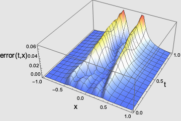
In this section, we provide the results of the potential approach applied to the price formation MFG system with quadratic cost and oscillating supply. We use the semi-explicit formulas introduced in [31] to assess the error in our approximation. We use the standard solver for finite-dimensional convex problems provided by the software Mathematica to approximate the potential function in a discrete grid in time and space.

Let $\kappa\in{\mathbb{R}}$ , $\eta\geqslant 0$ , and $c>0$ . For the quadratic cost configuration, we take

H(p)=\frac{1}{2c}p^{2},\quad V(x)=-\frac{\eta}{2}\left(x-\kappa\right)^{2},\quad\mbox{and}\quad u_{T}\left(x\right)\equiv 0.

Thus, $F(v)=\frac{c}{2}v^{2}$ . As shown in [31] and [30], a feature of the quadratic setting is the solvability of the Hamilton-Jacobi equation in (1.1) in the class of quadratic functions of $x$ with time-dependent coefficients

u(t,x)=a_{0}(t)+a_{1}(t)x+a_{2}(t)x^{2},\quad t\in[0,T],~x\in{\mathbb{R}}.

The coefficients $a_{0}$ , $a_{1}$ and $a_{2}$ solve an ODE system that derives from the Hamilton-Jacobi equation by matching powers of the $x$ variable. Figure 1(c) shows the value function for $(x,t)\in[0,T]\times[-1,1]$ . Moreover, the price has the following explicit formula

\varpi(t)=\eta\left(\kappa-\overline{m}_{0}\right)\left(T-t\right)-\eta\int_{t}^{T}\int_{0}^{s}Q(r)drds-cQ(t),\quad t\in[0,T],

where $\overline{m}_{0}=\int_{{\mathbb{R}}}xm_{0}(x)dx$ . The initial condition $m_{0}$ is centered at $x=0$ and with compact support $[-0.5,0.5]$ (see Figure 1(a)). The vector-field transporting $m_{0}$ is

b(t,x)=-\frac{1}{c}\left(\varpi(t)+a_{1}(t)+2a_{2}(t)x\right),\quad t\in[0,T],~x\in{\mathbb{R}},

which we use to compute $m$ using the method of characteristics (see Figure 2(b)). Thus, recalling (2.1) and (2.5), we have explicit formulas for $\varphi$ , $\varphi_{x}$ , and $\varphi_{t}$ . We use the previous expressions as a benchmark for the approximation obtained using (5).

For the discretization of the time variable, we set $T=1$ and $N_{t}=20$ time steps uniformly spaced. Thus, $h_{t}=0.05$ is the time step size. To discretize the space variable, the selection of $R$ in (4.11), where $R_{0}=0.5$ , becomes

R>\max\{5.57742~,\quad 0.811579\}.

However, to simplify the computational cost, we optimize the selection of $R$ by looking at the support of $m(t,)$ for $t\in[0,T]$ , which we illustrate in Figure 2(b). Thus, we discretize the space variable in the space domain $[-1,1]$ using $N_{x}=40$ time steps equally spaced. Thus, $h_{x}=0.05$ is the step size.

Because in several applications the supply function satisfies a mean reversion assumption, we assume that it follows the ordinary differential equation

\begin{cases}\dot{Q}(t)=\overline{Q}(t)-\alpha Q(t),&t\in[0,T],\\ Q(0)=q_{0},\end{cases}

where $\overline{Q}:[0,T]\to{\mathbb{R}}$ represents the average supply over time, $\alpha\in{\mathbb{R}}$ measures the tendency to towards the average, and $q_{0}\in{\mathbb{R}}$ is the initial supply. For numerical purposes, we select

\overline{Q}(t)=5\sin(3\pi t),\quad\alpha=4,\quad q_{0}=-0.5.

While the particular choice of $Q$ does not change the problem substantially, the preceding choice has oscillatory features, as we want to demonstrate how price changes and at the same time gives simple analytic expressions. As Figure 1(b) shows, the price inherits the oscillating behavior from the supply.

Using the solution $(u,m,\varpi)$ , we get $\varphi_{t}$ , $\varphi_{x}$ from (2.1) (see Figure 2(b)), and so (2.5) gives $\varphi$ , illustrated in Figure 2. The value of (4.16) is $0.106525$ , which we use as an additional benchmark to assess our numerical approximation.

We discretize (4.16) over the time-space grid using finite differences to approximate $\varphi_{t}$ and $\varphi_{x}$ ; that is

\varphi_{t}(t_{i},x_{j})=\dfrac{\varphi(t_{i}+h_{t},x_{j})-\varphi(t_{i},x_{j})}{h_{t}},\quad\varphi_{x}(t_{i},x_{j})=\dfrac{\varphi(t_{i},x_{j}+h_{x})-\varphi(t_{i},x_{j})}{h_{x}},

for $i=1,\ldots,20,$ and $j=1,\ldots,40$ . We obtain a finite-dimensional convex optimization problem with the following constraints

		$\displaystyle\varphi_{x}(t_{i},x_{j})\geqslant 0,\quad\sum_{j=1}^{N_{x}}\left(\varphi(t_{i},x_{j})-M_{0}(x_{j})\right)h_{x}+\sum_{k=0}^{i}Q(t_{k})h_{t},$
		$\displaystyle\varphi(0,x_{j})-M_{0}(x_{j})=0,\quad\varphi(t_{i},-1)=0,\quad\varphi(t_{i},1)=1,\quad i=1,\ldots,N_{t},\;j=1,\ldots,N_{x},$

which correspond to the discretization of the admissible set $\mathcal{A}(\Omega_{R})$ (see (4.14)). The results are depicted in Figure 3. The approximated value of (4.16) is $0.103765$ , in good agreement with the theoretical value $0.106525$ .

Using (5), we obtain the corresponding approximation of $\varpi$ , illustrated in Figure 4. Because of the implementation of finite differences, we can compute the price on the time horizon $[2h_{t},T]$ . The plots show good agreement between the values of our numerical results with a small discrepancy that improves as the grid size increases (here, we show the results for the finest grid we used).

As the last benchmark, we consider the value function $u$ . To compute $u$ , we round the approximation to avoid indeterminate expressions and we use (5.20). The result is depicted in Figure 5. Again, we obtain a good agreement with the exact solution.

7. Conclusions and further directions

In this paper, we presented a variational approach based on Poincaré Lemma, reducing one variable in the MFG price formation model. We studied the variational approach independently of the MFG problem. We obtained existence for a relaxed formulation using bounded variation functions, and we proved uniqueness of the potential function. We showed that price existence follows a Lagrange multiplier rule associated with the balance constrained, an integral equation for the MFG model depending on a supply function. For the price problem, the variational formulation allows an efficient computation without solving the backward-forward coupled problem with integral constraints. The convexity of the variational approach allows the use of standard optimization tools to solve its discrete formulation. Our numerical method shows promising results and good agreement with the explicit solutions. We consider we can apply a similar approach to the price formation model with common noise, which corresponds to the case of a stochastic supply function. One challenge is the dependence of the variational problem formulation on the supply, requiring the discretization of time, state variables, and the common noise. We plan to investigate this case in future works.

References

[1] Y. Achdou, F. Camilli, and I. Capuzzo-Dolcetta. Mean field games: numerical methods for the planning problem. SIAM J. Control Optim., 50(1):77–109, 2012.
[2] Y. Achdou and I. Capuzzo-Dolcetta. Mean field games: numerical methods. SIAM J. Numer. Anal., 48(3):1136–1162, 2010.
[3] Y. Achdou and M. Laurière. Mean Field Games and Applications: Numerical Aspects, pages 249–307. Springer International Publishing, Cham, 2020.
[4] R. Aïd, A. Cosso, and H. Pham. Equilibrium price in intraday electricity markets, 2020.
[5] R. Aïd, R. Dumitrescu, and P. Tankov. The entry and exit game in the electricity markets: A mean-field game approach. Journal of Dynamics & Games, 8(4):331–358, 2021.
[6] C. Alasseur, I. Ben Taher, and A. Matoussi. An extended mean field game for storage in smart grids. Journal of Optimization Theory and Applications, 184(2):644–670, 2020.
[7] C. Alasseur, L. Campi, R. Dumitrescu, and J. Zeng. Mfg model with a long-lived penalty at random jump times: application to demand side management for electricity contracts, 2021.
[8] A. Alharbi, T. Bakaryan, R. Cabral, S. Campi, N. Christoffersen, P. Colusso, O. Costa, S. Duisembay, R. Ferreira, D. Gomes, S. Guo, J. Gutierrez, P. Havor, M. Mascherpa, S. Portaro, R. Ricardo de Lima, F. Rodriguez, J. Ruiz, F. Saleh, S. Calum, T. Tada, X. Yang, and Z. Wróblewska. A price model with finitely many agents. Bulletin of the Portuguese Mathematical Society, 2019.
[9] L. Ambrosio, N. Fusco, and D. Pallara. Functions of bounded variation and free discontinuity problems. Oxford Mathematical Monographs. The Clarendon Press, Oxford University Press, New York, 2000.
[10] Y. Ashrafyan, T. Bakaryan, D. Gomes, and J. Gutierrez. A duality approach to a price formation mfg model, 2021.
[11] H. Attouch, G. Buttazzo, and G. Michaille. Variational analysis in Sobolev and BV spaces: applications to PDEs and optimization. SIAM, 2014.
[12] T. Bakaryan, R. Ferreira, and D. Gomes. A Potential Approach for Planning Mean-Field Games in One Dimension . Submitted to Communications on Pure and Applied Analysis, 2021.
[13] T. Basar and R. Srikant. Revenue-maximizing pricing and capacity expansion in a many-users regime. In Proceedings.Twenty-First Annual Joint Conference of the IEEE Computer and Communications Societies, volume 1, pages 294–301 vol.1, 2002.
[14] F. Bonnans, P. Lavigne, and L. Pfeiffer. Discrete potential mean field games, 2021.
[15] L. Caravenna and G. Crippa. Uniqueness and lagrangianity for solutions with lack of integrability of the continuity equation. Comptes Rendus Mathematique, 354(12):1168–1173, 2016.
[16] P. Cardaliaguet. A short course on mean field games. 2018.
[17] R. Carmona and M. Laurière. Convergence analysis of machine learning algorithms for the numerical solution of mean field control and games I: the ergodic case. SIAM Journal on Numerical Analysis, 59(3):1455–1485, 2021.
[18] R. Carmona and M. Laurière. Convergence analysis of machine learning algorithms for the numerical solution of mean field control and games II: The finite horizon case. To appear in Annals of Applied Probability, 2021.
[19] G. Csató, B. Dacorogna, and O. Kneuss. The Pullback Equation for Differential Forms. Progress in Nonlinear Differential Equations and their Applications. Birkhäuser/Springer, New York, 2012.
[20] G. Dal Maso. An introduction to G-convergence. Progress in Nonlinear Differential Equations and Their Applications. Birkhäuser Boston, 1 edition, 1993.
[21] B. Djehiche, J. Barreiro-Gomez, and H. Tembine. Price Dynamics for Electricity in Smart Grid Via Mean-Field-Type Games. Dynamic Games and Applications, 10(4):798–818, December 2020.
[22] L. C. Evans. Partial Differential Equations. Graduate Studies in Mathematics. American Mathematical Society, 1998.
[23] L. C. Evans and R. F. Gariepy. Measure Theory and Fine Properties of Functions, Revised Edition. Textbooks in Mathematics. CRC Press, 2015.
[24] O. Féron, P. Tankov, and L. Tinsi. Price Formation and Optimal Trading in Intraday Electricity Markets with a Major Player. Risks, 8(4):1–1, December 2020.
[25] O. Féron, P. Tankov, and L. Tinsi. Price formation and optimal trading in intraday electricity markets, 2021.
[26] I. Fonseca and G. Leoni. Modern methods in the calculus of variations: $L^{p}$ spaces. Springer Monographs in Mathematics. Springer, New York, 2007.
[27] M. Fujii and A. Takahashi. A Mean Field Game Approach to Equilibrium Pricing with Market Clearing Condition. Papers 2003.03035, arXiv.org, March 2020.
[28] M. Fujii and A. Takahashi. Equilibrium price formation with a major player and its mean field limit, 2021.
[29] D. Gomes, J. Gutierrez, and R. Ribeiro. A mean field game price model with noise. Math. Eng., 3(4):Paper No. 028, 14, 2021.
[30] D. Gomes, J. Gutierrez, and R. Ribeiro. A random-supply mean field game price model, 2021.
[31] D. Gomes and J. Saúde. A Mean-Field Game Approach to Price Formation. Dyn. Games Appl., 11(1):29–53, 2021.
[32] W. Kirsch. A survey on the method of moments. 2015.
[33] J.-M. Lasry and P.-L. Lions. Jeux à champ moyen. II. Horizon fini et contrôle optimal. C. R. Math. Acad. Sci. Paris, 343(10):679–684, 2006.
[34] A. Lin, S. Fung, W. Li, L. Nurbekyan, and S. Osher. Alternating the population and control neural networks to solve high-dimensional stochastic mean-field games. Proceedings of the National Academy of Sciences, 118(31), 2021.
[35] C. Mou, X. Yang, and C. Zhou. Numerical methods for mean field games based on gaussian processes and fourier features, 2021.
[36] C. Orrieri, A. Porretta, and G. Savaré. A variational approach to the mean field planning problem. J. Funct. Anal., 277(6):1868–1957, 2019.
[37] L. Perko. Differential Equations and Dynamical Systems, Third Edition. 3rd edition, 2006.
[38] B. Perthame. Transport equations in biology. Frontiers in Mathematics. Birkhäuser Verlag, Basel, 2007.
[39] L. Ruthotto, S. Osher, W. Li, L. Nurbekyan, and S. Fung. A machine learning framework for solving high-dimensional mean field game and mean field control problems, 2020.
[40] H. Shen and T. Basar. Pricing under information asymmetry for a large population of users. Telecommun. Syst., 47(1-2):123–136, 2011.
[41] A. Shrivats, D. Firoozi, and S. Jaimungal. A Mean-Field Game Approach to Equilibrium Pricing, Optimal Generation, and Trading in Solar Renewable Energy Certificate Markets. Papers 2003.04938, arXiv.org, March 2020.

	$\displaystyle\int_{0}^{T}\int_{-R}^{R}\bigg(\left(L^{}_{z}(t,x)\right)_{t}+\left(L^{}_{y}(t,x)-V(x)\right)_{x}\bigg)\left(\psi(t,x)-\varphi(t,x)-\varphi_{x}(t,x)\left(\overline{x}(t)-\overline{z}(t)\right)\right){\rm d}x{\rm d}t$
	$\displaystyle=\int_{0}^{T}\int_{-R}^{R}\bigg(\left(L^{}_{z}(t,x)\right)_{t}+\left(L^{}_{y}(t,x)-V(x)\right)_{x}$
(5.14)		$\displaystyle\quad\quad\quad\quad\quad-\int_{-R}^{R}\bigg(\left(L^{}_{z}(t,y)\right)_{t}+\left(L^{}_{y}(t,y)-V(y)\right)_{x}\bigg)\varphi_{x}(t,y){\rm d}y\bigg)\left(\psi(t,x)-\varphi(t,x)\right){\rm d}x{\rm d}t.$