A study of photoionized gas in two Hii regions of the N44 complex in the LMC using MUSE observationsJournal: ApJ
Abstract
We use the optical integral field observations with Multi-Unit Spectroscopic Explorer (MUSE) on the Very Large Telescope, together with CLOUDY photoionization models to study ionization structure and physical conditions of two luminous H ii regions in N44 star-forming complex of the Large Magellanic Cloud. The spectral maps of various emission lines reveal a stratified ionization geometry in N44 D1. The spatial distribution of [O i] 6300Å emission in N44 D1 indicates a partially covered ionization front at the outer boundary of the H ii region. These observations reveal that N44 D1 is a Blister H ii region. The [O i] 6300Å emission in N44 C does not provide a well-defined ionization front at the boundary, while patches of [S ii] 6717Å and [O i] 6300Å emission bars are found in the interior. The results of spatially resolved MUSE spectra are tested with the photoionization models for the first time in these H ii regions. A spherically symmetric ionization-bounded model with a partial covering factor, which is appropriate for a Blister H ii region can well reproduce the observed geometry and most of the diagnostic line ratios in N44 D1. Similarly, in N44 C we apply a low density and optically thin model based on the observational signatures. Our modeling results show that the ionization structure and physical conditions of N44 D1 are mainly determined by the radiation from an O5 V star. However, local X-rays, possibly from supernovae or stellar wind, play a key role. In N44 C, the main contribution is from three ionizing stars.
Keywords:
Interstellar line emission (844), Photoionization (2060), Large Magellanic Cloud (903), H ii regions (694)I Introduction
Massive stars are the significant sources of ultraviolet (UV) radiation in galaxies with energies high enough ( 13.6 eV) to ionize the neutral gas in the interstellar medium (ISM). A part of this high-energy radiation is absorbed by the neutral gas and heats the surrounding medium creating the ionized H ii regions. A large fraction of this ionizing radiation escapes into the diffuse medium, penetrating the molecular gas, if some part of the H ii region is optically thin. This creates an ionization zone (H+), ionization front (H0), and a photodissociation region (PDR). The ionization front is at the outer boundary of an H ii region that lies inside the PDR. There have been several studies of Galactic and extragalactic H ii regions and PDRs, e.g., Orion Nebula (Pogge et al. 1992; García-Díaz & Henney 2007), 30 Doradus (Pellegrini et al. 2010), NGC 364 (Peimbert et al. 2000; Relano et al. 2002), dense H ii regions in IC 10 (Polles et al. 2019) and NGC 595 (Relaño et al. 2010). The impact of ionizing radiation on the surrounding medium and the physical properties of H ii regions are normally obtained by strong emission lines in the optical spectrum, which is mainly populated by hydrogen recombination lines and forbidden lines of other common elements. These gas emission lines are sensitive to physical conditions such as density and temperature; hence their relative intensities can probe the physical mechanism involved in the ionization processes.
The Large Magellanic Cloud (LMC) is an ideal laboratory to study the properties of H ii regions and the massive star feedback in a low-metallicity galaxy due to its sub-solar metallicity ( Z = 0.5Z⊙, Westerlund 1997); face-on viewing angle (van der Marel & Cioni 2001); reduced extinction along the line of sight; a distance of 50 kpc (Pietrzyński et al. 2019) allowing the spatially resolved observations of the ISM structures on sub-parsec scales. Naslim et al. 2015 have reported on ten PDRs in the LMC using H2 pure rotational transition emission obtained with Spitzer. These regions include intense H ii regions, diffuse ISM clouds, and dense molecular clouds. We study the individual clouds in detail using various observations to investigate the high-mass star formation (see Naslim et al. 2018; Nayana et al. 2020) and its impact on the ISM. To explore the impact of ionizing radiation from massive stars on the surrounding medium, we revisit two H ii regions in a well-studied star-forming complex of the LMC, N44. We examine the physical conditions and ionization structure of N44D and N44C by comparing the observations with the predictions of the photoionization model, CLOUDY (Ferland et al. 2017).
The N44 superbubble is one of the brightest star-forming regions in the LMC, which can be clearly traced by its compact H ii regions along the main shell rim in an H map (Fig. 1). The region is powered by nearly 3538 hot stars (Oey & Massey 1995; McLeod et al. 2019) of stellar associations LH47, LH48 and LH49 (Lucke & Hodge 1970). McLeod et al. 2019 report the analysis of radiative and mechanical feedback from massive stars in the H ii regions of N44 (N44 A, N44 B, N44 C and N44 D) using the optical integral field data from Multi-Unit Spectroscopic Explorer (MUSE). They used He ii 5412Å line to identify the feedback driving massive stars, and estimated the spectral types and luminosity classes of these stars for determining the stellar radiative output. Using the nebular emission line maps of H, H, [S ii] 6717, 6732Å, [N ii] 6584Å, and [O iii] 5007Å, they derived the electron density from [S ii] 6717/6732 ratio assuming a nebular electron temperature of 10 000 K. They also derived the degree of ionization using [O ii]/[O iii] ratio, kinematics, and the oxygen abundances. In addition, they explored the role of different stellar feedback mechanisms by estimating various pressures and found that the H ii region expansion is mainly driven by stellar radiation pressure and ionized gas.
In this paper, we further explore the rich nebular emission lines in MUSE data set (McLeod et al. 2019) of N44 for a detailed understanding of their spatial distributions, ionization structures and physical conditions. We compare these results with the photoionization models to interpret the observations of this star-forming complex. The MUSE archival data of N44 provides many iconic emission lines, such as H, H, [S iii] 9069Å, [S ii] 6717, 6732Å, [O iii] 4959, 5007Å, [O ii] 7318, 7329Å, [O i] 6300Å, and [N ii] 6584Å, that have only been partially utilized in McLeod et al. 2019. We exploit various emission line ratios to study the behavior of different ionization zones and compare the observed line ratios with the best-fit photoionization models to further understand the physical process.
The N44 main shell is surrounded by several H bright regions (Fig. 1). The compact H ii region on the southwest rim of the shell, N44 D, is the most luminous one in N44 (McLeod et al. 2019). We choose two brightest H ii regions N44 D and N44 C for our study, which show higher degree of ionization than N44 A and N44 B, and nearly spherical ionization structures with different feedback characteristics based on studies by McLeod et al. 2019. N44 D encloses three hot stars of spectral types O5 V, O9.5 V and O5.5 V (McLeod et al. 2019). The second brightest H ii region, N44 C, is adjacent to N44D on the western rim of the shell, and the region harbors three hot stars O5 III, O9.5 V and O5 III (McLeod et al. 2019). One reason for selecting N44 D is that MUSE observations show an edge on ionization front, allowing a detailed study of ionization as a function of depth into the cloud. At first glance, N44 C does not show such a well-defined ionization front at the H ii region boundary, while it shows a higher photon escape fraction relative to N44 D that reported by McLeod et al. 2019. These two nebulae show different ionization structures, hence physical process of two different types of H ii regions can be compared. Moreover, the hot star content of N44 H ii regions are extensively studied and high-spatial-resolution observations are readily available. This study allows us to directly apply the observed stellar parameters, gas densities, and emission line intensities to constrain the photoionization model without arbitrary assumption, and test their influence on geometry of the H ii regions.

II Observations
We used the MUSE archival data of N44 C and N44 D (program ID: 096.C-0137(A), PI: A. F. McLeod). MUSE is a large field-of-view (FOV) integral field unit (IFU) panchromatic optical instrument on the European Southern Observatory’s (ESO’s) Very Large Telescope (VLT) in Paranal, Chile. This instrument provides high-spatial-resolution observations at a pixel scale of 0.2′′ with a resolving power ranging from 1770 to 3590. The observations of N44 C and N44 D have been taken on 21 October 2015 and 25 February 2016, with the MUSEwfm-noaoobsgenericoffset observing template, in a wide-field observing mode covering a wavelength range 475935 nm. The reduced MUSE data is retrieved from the ESO science archive11 1 http://archive.eso.org/cms.html. The data were reduced using the MUSE-1.6.1 pipeline. The MUSE pipeline process automatically removes most of the instrumental signatures. The raw data were pre-processed, and bias subtraction, flat fielding, sky-subtraction, wavelength calibration and flux calibration were applied. These data were not taken with the Adaptive Optics System of MUSE and the seeing-limited angular resolutions 0.98′′ and 1.30′′ are achieved for N44D and N44C respectively. We note that, no point spread function (PSF) matching was applied for subsequent analysis and all the analysed regions are resolved regardless of the achieved seeing. Our analysis is based on integrated line flux maps, hence no PSF information is retained.
III Emission line maps of N44 D and N44 C
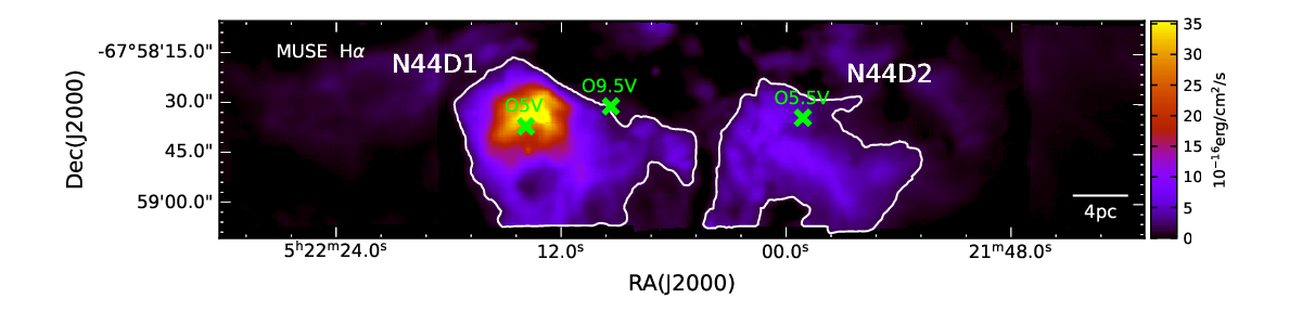
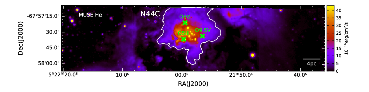
Fig. 2 shows the extinction corrected H line flux maps of N44 D and N44 C obtained with MUSE. The ionized gas traced by the H emission shows two H ii regions in N44 D, those we label as N44 D1 and N44 D2, and one in N44 C. Even though the regions are nearly spherical, their boundaries cannot be directly specified in a circular aperture. Hence for determining the boundaries of these H bright regions based on their surface brightness, we use the Python package ASTRODENDRO (Rosolowsky et al. 2008). This algorithm identifies and characterizes the hierarchical structures in the emission line map as a structure tree, where each entity is represented as an isosurface. The local maxima represent the top level of the dendrogram and are identified from the emission line map with the flux 3. The isosurfaces (two-dimensional contours) that surround the local maxima are leaves, branches, and trunks. The trunks represent parent structures that enclose the branches connecting two leaves. Further description and methods of using ASTRODENDRO can be found in Naslim et al. 2018. Della Bruna et al. 2020 have recently used ASTRODENRO to identify H bright regions in MUSE maps of NGC 7793 by applying a similar method. We define the boundary of H ii regions in H map that are identified as trunks with ASTRODENDRO. The lower contour levels of these trunks are taken as the boundaries of H ii regions within the chosen observation field. These regions appear as polygons in Fig. 2.


In addition to H 6562.8Å emission, the MUSE spectra of N44 D1 and N44 C show emission due to H 4861Å, [O iii] 5007Å, 4959Å, [O ii] 7318Å, 7329Å, [O i] 6300Å, [N ii] 6584Å, [S ii] 6717Å, 6732Å, [S iii] 9069Å, [Ar iii] 7135Å, 7751Å and many He i and Paschen hydrogen lines ( Fig 3). Fig. 6 shows integrated line flux maps of H, [S ii] 6717Å, [O iii] 5007Å, [O ii] 7318Å, [O i] 6300Å, and [N ii] 6584Å in N44 D1, N44 D2, and N44 C. H and [O iii] 5007Å emission show similar spatial distribution as the H emission in both N44 D and N44 C, whilst [S ii], [O ii], [N ii] and [O i] emission in N44 D1 show a shell structure. The morphology of N44 D2 is irregular with pillars or filamentary structures. The continuum subtraction is applied by creating continuum maps from the user defined line-free portions of the spectrum around each emission line. The line fluxes (erg s-1 cm-2) of N44 D1, N44 D2 and N44 C regions are then extracted from the integrated line flux maps by applying aperture photometry within the specified regions as polygon structures obtained from ASTRODENDRO. Only the pixel values with S/N 10 are considered within all the polygons. These fluxes are then point source flux removed by subtracting the point source fluxes, which are also extracted within the user defined apertures. For uncertainties, we added in quadrature the error in aperture photometry, and an expected 20 calibration error in every line flux measurements. The error in photometry is the quadratically added uncertainty in measurements over all pixels within a region.
To check the data reduction and flux calibration quality of data cube retrieved from the MUSE archive, we compared the H line luminosities (erg s-1) of N44 C and N44 D1 from the MUSE archival data to the H luminosities presented in McLeod et al. 2019. In Table 1 we show the comparison of H luminosities obtained from the data presented in this work and McLeod et al. 2019. We note that the line luminosities obtained from the two data sets agree within the estimated uncertainties, hence we are confident to proceed with the analysis of pipeline reduced MUSE archival data. The observed line luminosities (erg s-1) are given in Table 2. We choose two bright regions, N44 D1 and N44 C, for further analysis with photoionization models.
. N44 D1 N44 C (ergs-1) (erg s-1) (erg s-1) (erg s-1) 1037) (1037) (1037) (1037) 1.470.16 1.47 1.390.15 1.51
a: MUSE archival data used in this work. b: McLeod et al. 2019.
IV Emission line ratios: [S II]/H, [N II]/H, [O III]/H and [O III]/H
We present the extinction corrected [S ii] 6717/H, [N ii] 6584/H, [O iii] 5007/H, and [O iii] 5007/H ratio maps of N44 D and N44 C in Figs. 4 and 5, respectively. These ratios allow us to study the ionization structure of the region. [S ii] 6717/H and [N ii] 6584/H are lower at the central regions closer to the ionizing stars implying a higher ionization zone, while at the periphery the values of these ratios are higher indicating low ionization zone. We find that both [S ii] 6717/H and [N ii] 6584/H maps of N44 D1 and N44 C show a shell morphology. The central part of the N44 D1 has a lower [S ii] 6717/H ratio ( 0.02), and at the periphery, its value is 0.3. N44 C shows a [S ii] 6717/H value of 0.04 at the center and a value of 0.20 at the periphery. Similarly, the value of [N ii] 6584/H ratio ranges from 0.03 to 0.20 in N44 D1, and 0.04 to 0.15 in N44 C. The model calculations by Allen et al. 2008 have shown that [S ii]/H and [N ii]/H ratios greater than 0.39 and 0.79 would be a result of strong contributions from shocks. The [S ii]/H and [N ii]/H ratios of both N44 D1 and N44 C are well below the values 0.39 and 0.79, respectively, indicating a substantial contribution from photoionization. However, in the regions outside the boundary of these H ii regions, we find the enhanced [S ii]/H and [N ii]/H ratios; hence the contribution from shocks cannot be totally ignored.
A similar effect is found in the [O iii] 5007/H and [O iii] 5007/H ratios. The values are higher in the regions closer to the central ionizing stars showing a high degree of ionization, while the ratios are lower at the outer regions indicating a low degree of ionization. We note that, the integrated [O iii] 5007/H ratio of N44 D1 (2.52) is much higher than N44 D2 (1.67) and N44 C (0.55), which indicates the hardness of radiation field in N44 D1. The [O iii] 5007/H ratio is also higher in N44 D1, representing the effect of high effective temperature of the ionizing star of spectral type O5 V. The N44 D1, N44 D2, and N44 C show an [O iii] 5007/H ratio of 7.89, 5.18 and 2.07 respectively. In N44 C, the high values of [O iii] 5007/H ( 1.0 – 0.3) and [O iii] 5007/H ( 3.0 – 1.0) are near the O5 III star and the values decrease toward the edge of the bubble.


V H and H emission
V.1 Extinction correction
The line luminosities are corrected for extinction using the intensity ratios (H/H). Since, H/H ratio is relatively sensitive to temperature, it can be used as a reliable reddening indicator. This ratio is compared with the theoretically expected value of the Balmer decrement (H/H for Case B recombination (Osterbrock & Ferland 2006). Any deviation from expected value of H/H ratio for a particular electron temperature can be associated with extinction. We estimate the nebular emission line color excess from the H/H ratio using the equation from Domínguez et al. 2013,
| (1) |
The expected value of (H/H flux ratio is 2.86 (Osterbrock & Ferland 2006). This value is obtained by assuming Case B recombination at an electron temperature 10 000 K and density 100 cm-3. Then, following the extinction curve estimated by Calzetti et al. 2000,
| (2) |
for = 0.63 to 2.2 , and
| (3) |
for = 0.12 to 0.63 .
Here, and are the extinction curves at H and H wavelengths respectively.
Assuming the ratio of total to selective extinction , which is valid at optical wavelength for the LMC (Gordon et al. 2003), we get = 2.38 , and = 3.65 .
Using the color excess , the extinction in magnitude for H line is obtained by
| (4) |
and for H line,
| (5) |
Then extinction corrected H luminosity, (H is,
| (6) |
and the extinction corrected H luminosity, (H is,
| (7) |
Here (H and (H are the observed luminosities of H and H emission respectively.
The values of the color excess are 0.08 for N44 D1 and N44 D2, and 0.20 for N44 C. The extinction toward N44 D1 is mag. Our value agrees with the calculations by Garnett et al. 2000 and Lopez et al. 2014 for N44. The N44 C has a significantly higher extinction, mag.
We applied the same method of extinction correction to other line emission, and the extinction corrected luminosities (erg s-1) are given in Table 2.
V.2 Lyman Continuum Photon Flux
The O-type stars in H ii regions are the prominent sources of Lyman continuum photons. These stars deposit a bulk of their high energy photons into the surrounding H ii region within the Stromgren radii. If the gas is optically thick in the Lyman continuum, we expect all the ionizing photons emitted by the star to be absorbed. However, a significant fraction of these photons can escape on a larger scale outside of the H ii region into the ISM. This fraction of photon leakage from H ii regions needs to be measured to understand the overall energy budget, and to probe whether the dominant hot stars in the region are responsible for the photoionization in the surrounding medium. We calculate the number of L[OIII]/Hyman continuum photons () absorbed in the region surrounding a hot star corresponding to H luminosities by assuming the Case B recombination for electron temprature = 10 000 K, and density = 100 cm-3. The number of Lyman continuum photon related to H luminosity is obtained by = 7.3110(H) ph s-1 (Kennicutt 1998; Osterbrock & Ferland 2006).
The number of ionizing photons derived from the H luminosity () for N44 D1, N44 D2, and N44 C are tabulated in Table 3. To calculate the photon escape fraction, we also need to know the number of total Lyman continuum photons emitted by the ionizing stars. We adopt the model calculations () for hot stars of appropriate spectral types from Martins et al. 2005. The values of the only O5 V star in N44 D1, a combination of three ionizing stars of spectral types O5 III, O8 V and O9.5 V in N44 C, and O5.5 V star in N44 D2 are given in Table 3.
Using the and values we calculate the photon escape fraction,
| (8) |
McLeod et al. 2019 reported 0.37 and 0.68 for N44 D1 and N44 C respectively, using this method. We verify their determination and find that for N44 D1, N44 D2, and N44 C are 0.36, 0.71, and 0.70 respectively. These values imply that about 36 of the ionizing photons escape from N44 D1, 71 of ionizing photons escape from N44 D2 and 70 from N44 C. N44 C shows a relatively larger amount of photon leakage than N44 D1, and is more optically thin to the ionizing photon. This observation is consistent with the study of H ii regions in the LMC by Pellegrini et al. 2012 that boundaries of optically thick regions are generally characterized by stratification in the ionization structures. The ionization structure of N44 D1 shows a well-defined nebular boundary where [O i] and [S ii] emission peak at the outer boundary of the H and [O iii] emission. The [S ii]/H ratio map clearly shows the transition region in the ionization structure. N44 C does not show such an ionization stratification, while a slightly extended shell structure is found in the [S ii]/H map.
Using the number of ionizing photons , we can also estimate the average electron density of emitting gas in an H ii regions, . Assuming the spherical nebula where H is fully ionized, the recombination balance equation is,
| (9) |
Here is the Case B recombination coefficient 2.5910-13 cm3 s-1 for gas at = 10 000 K. is the mean radius of t[OIII]/Hhe H ii region. Then the average electron density from H emission is obtained by,
| (10) |
Here (=Q/1048) is the number of Lyman continuum photons derived from the H luminosity and is the radius in parsec. The derived from H emission of N44 D1, N44 D2, and N44 C are 31, 26, and 38 cm-3 respectively.
V.3 Electron density
Electron density () and electron temperature () are two important physical parameters for characterizing an H ii region. The can be determined from the observed line intensities of two different energy levels with nearly equal excitation energy of the same ion. Their line ratios are generally not sensitive to . The forbidden lines ratio, [S ii] 6717/6732 is usually used to determine , where [S ii] 6717Å and 6732Å emission are relatively strong in the ionized nebula. Their corresponding critical density is 103 cm-3, hence probing the low-density regimes. McLeod et al. 2019 have reported cm-3 for N44 C and cm-3 for N44 D1, applying the analytical solution given in McCall 1984 and assuming a of 10 000 K. Toribio San Cipriano et al. 2017 have derived cm-3 for a 3.09.4 arcsec2 region closer to the ionizing star in N44 D1 using [S ii] 6717/6732 ratio obtained from VLT-UVES spectrum. Lopez et al. 2014 have reported a relatively low value of cm-3 for the entire N44 using the flux density of the free-free emission at 3.5 cm. Garnett et al. 2000 derived for N44D1 using [S ii] 6717/6732 ratio obtained with 0.9 m telescope at Cerro Tololo Inter-American Observatory. McLeod et al. 2019 emphasize that, densities derived from radio emission by Lopez et al. 2014 are expected to be smaller than those derived from the ratio of collisionally excited lines (Peimbert et al. 2017). These studies show a discrepancy in derived values of for N44 D1 and N44 C, hence we calculate the electron densities using [S ii] 6717/6732 ratios of N44 D1 and N44 C derived in our analysis of MUSE spectra. Electron temperature can be obtained by the forbidden line ratios [SIII]6312/9069 and [NII]5755/6384, however the MUSE observations of N44 D1 and N44 C show very weak [SIII] 6312Å and [NII] 5755Å emission, which cannot be extracted from the data cube within a 5 detection threshold in most of the pixels inside the defined polygons. We calculate the electron density as in McLeod et al. 2015 by applying the analytical solution in McCall 1984.
| (11) |
Here, R is the [S ii] 6717/6732 ratio, and electron temperature is assumed to be 10 000 K as in McLeod et al. 2019. The derived for N44D1, N44D2 and N44C using this method are 14143, 12137 and 9235 cm-3 respectively. We also estimate using the publicly available Python based package, PYNEB (Luridiana et al. 2013) for a comparison. This algorithm includes FIVEL (De Robertis et al. 1987) and NEBULAR (Shaw & Dufour 1995) packages for analyzing nebular emission lines. The package calculates the physical conditions ( and ) for a given set of emission line intensities, and returns the diagnostic plots. We use the density sensitive [S ii] 6732/6717 line ratio to determine using the diags.getTemDen task in PYNEB for a given of 10 000 K. The estimated electron densities from PYNEB for N44D1, N44D2 and N44C are 13250, 11545 and 6640 cm-3 respectively (Table 3). These density values are comparable with the density derived from the equation 11 within the estimated uncertainties.
VI Structure of ionized gas


To investigate the structure of ionization zones in N44 D and N44 C we compare the spatial distribution of H, [O iii], [O ii], [O i], [N ii] and [S ii] emission line maps (Fig. 6). The spatial distribution of [O iii], [O ii], and [O i] of N44 D1 in Fig. 6(a) shows a clear stratification from ionization zones where [O iii] 5007Å emission peaks around the O5 V star, to the [O i] 6300Å emission at the ionization front. O’Dell & Wen 1992 have reported that [O i] 6300Å emission arises at the ionization front behind the PDR, between the ionization zone and molecular cloud. The majority of the [O i] 6300Å emission in H ii regions is due to the collisional excitation by thermal electrons and atomic hydrogen via the charge exchange, hence the intensity of [O i] 6300Å emission can be a measure of neutral hydrogen content. [O i] 6300Å in PDRs can also be collisionally excited by electrons ejected by dust grains and Polycyclic Aromatic Hydrocarbon (PAHs) that absorb far-UV radiation emitted by the massive stars. In Fig. 6(b), we compare the spatial distribution of H (blue) and [N ii] 6584Å(red) with [S ii] 6717Å(green). [S ii] emission is expected to peak at ionization front. [N ii] emission is found to be co-spatial with [O ii] emission that peaks at partial-ionization zone, and concentrated in the outer boundary of the H and [O iii] emission. The structure of N44 D1 is nearly spherical with only one important source of ionizing photons.
In Fig. 7 we show the spatial profiles of various nebular emission lines by taking a cross-cut along the north-western edge of N44 D1. [O ii] and [N ii] emission are in a thin layer at the partial ionization zone outside [O iii], but slightly interior to the [O i] emission. The [O i] emission is concentrated in a thin zone 4 – 7 pc located in the outer boundary of the H ii region. H, H, [O iii] and He i are found to be co-spatial in the ionization zone. In the outer layer of the ionization front in this H ii region, we expect a well-defined PDR with a layer of C ii, then H2 emission, and a molecular cloud. High-spatial resolution spectroscopic observations in infrared and submillimeter wavelengths are required for further studies of PDR properties. A similar ionization structure is reported in the Orion Nebula H ii region. The [O i] 6300Å and [S ii] 6717Å emission appear to peak along a bright bar at the ionization front in the outer boundary, that forms a thin transition layer of thickness 1015–1016 cm between the ionization zone and PDR.The emission from higher ionization species [O iii] arises away from the ionization front close to the ionizing star Ori C (O’Dell et al. 2017; O’Dell 2001; Hester 1991; O’Dell & Wen 1992).
In N44 C, the [O iii] 5007Å and H emission appear to peak in the interior of the bubble near the ionizing star O5 III (Figs. 6 c, d). We show the spatial profiles of [O iii], [O ii], [S ii], [N ii], and H emission in N44 C taking a cross-cut from the position centroid of three ionizing stars to the north-east of N44 C (Fig. 7). The spatial distribution of [O iii] 5007Å and H, are similar and co-spatial in the fully ionized zone. [O i] 6300Å, [O ii] 7318Å, [N ii] 6584Å and [S ii] 6717Å emission do not form a well-defined outer boundary, but appear as patches of emission bars within [O iii] 5007Å and H emission region.
VII Comparison with photoionization model
The MUSE observations of N44 in the LMC show that the two bright H ii regions N44 D1 and N44 C have different ionization geometries and physical characteristics. N44 D1 has H and H surface brightness values 0.03 dex and 0.1 dex higher than N44 C. [O iii]/H and [O iii]/H ratios in N44 D1 are considerably larger than in N44 C, indicating a higher degree of ionization. N44 D1 shows a higher [O i] 6300/H ratio with a well-defined [O i] 6300Å emission at the H ii region outer boundary, indicating an ionization front.
In the ideal case, the [O i] 6300Å emission dominates at the outer boundary of the H ii region where the neutral hydrogen density dominates; hence we expect most of the Lyman continuum photons are absorbed by the nebula is ionization-bounded. This is an optically thick case, where we find a shell of [O i] 6300Å emission at the ionization front, indicating the border of the H ii region. In the density-bounded H ii regions, there is no well-defined ionization front surrounding highly ionized gas, and most of the Lyman continuum photons leak from the cloud contributing to the diffuse ionized gas outside of the cloud. In such cases, there is a weak [O i] 6300Å emission condensation within the H ii region or no shell structure at the boundary. In a Blister H ii region, there is a partial ionization front at the boundary, which does not cover the nebula completely; hence the photons escape in certain directions. Our study of the [O i] 6300Å emission in N44 D1 and N44 C reveals these different observational properties of H ii regions. Moreover, the measurement of the photon leakage using the H emission indicates that N44 D1 and N44 C have photon escape fractions 36 and 70, respectively. These calculations are in agreement with the study of the photon leakage by McLeod et al. 2019. The remaining ionizing photons are trapped within the H ii region itself and affect the overall ionization balance. Pellegrini et al. 2011; Pellegrini et al. 2012 reported that the ionization-bounded H ii regions are constrained to an escape fraction 0.6 and those with density-bounded are 0.6.
To further interpret these observations, we compute various photo-ionization models for comparing the emission line ratios and the geometry of ionization structure. We model the ionization structure of N44 D1 and N44 C using the photoionization code CLOUDY (Ferland et al. 2017). We derive the emissivities of prominent ionic species across the H ii region, from the illuminated face of the H+ region through the partially ionized zone to the neutral ionization front, where ionizing radiation has been attenuated and becoming neutral to the molecular zone. We develop various photoionization models for N44 D1 and N44 C, and test which model can better match the observed ionization geometry of the cloud and emission line ratios. To compare the ionization geometry, we use the spatial profiles of the line emissions along the H ii regions (Figs. 7 and 8). The emission line ratios we use for tests are given in Tables 4 and 5. The [S ii] 6717/6732 line ratio is sensitive to electron density, and [O ii] (7318+7329)/[O iii] 5007 to the ionization parameter. [O iii] 5007/H, [O iii] 5007/H, [O ii]/H, [N ii]/H, and [O i]/H give the behavior of different ionization zones, and are also sensitive to the metallicity. These line ratios are very sensitive to the adopted input parameters. A built-in optimization program based on the PHYMIR algorithm (van Hoof 1997; van Hoof et al. 2013; Ferland et al. 2013) is used to obtain the best fit model, which applies a minimization to determine the goodness-of-fit by varying the input parameters. We vary the total hydrogen density (), (H), and filling factor to find the best agreement between the model with the observed line ratios and geometry. Sometimes, for a given set of constraints some observables are optimized very well compared to the other sets and the best-fit model is obtained by the overall . Therefore, we manually fine tuned certain parameters until the best matching line ratios with the observations are obtained. Finally, the model line ratios are compared with the observed line ratios and the best-fit model was determined by calculating the as (Mondal et al. 2017; Pavana et al. 2019),
| (12) |
Here, the number of observed lines is n, Mi is the model line ratio, Oi is the observed line ratio and the is the error in the observed flux ratio. The best optimized model line ratios, observed line ratios and the values are given in Tables 4 and 5.
The basic input parameters to CLOUDY require the geometry of the cloud, intensity of incident ionizing photon flux, elemental abundances and gas density.
VII.1 Geometry
Observations show a clear ionization stratification in N44 D1. The ionized gas is traced by [O iii] 5007Å and H emission and the ionization front is traced by [O i] 6300Å and [S ii] 6717Å emission. The line ratio maps show a nearly radial symmetry around the ionizing star. This structure is quite simple to model as observation shows there is only a prominent source of the ionizing photon at the cloud’s interior. For N44 D1, we calculate an optically thick spherical model with a covering factor 0.64. We choose an outer radius, = 7.4 pc based on the observed geometry (Fig. 7). McLeod et al. 2019 report a radius containing 90 per cent of the H emission, = 7.4 pc for N44 D1 which agrees with the adopted radius in our model. The model constitutes the exciting star at the center of a spherical cloud, surrounded by the layers of H ii region and PDR.
MUSE observation of N44 C does not show a clear ionization stratification as N44 D1. However, observations indicate that the majority of photons escape from N44 C and the region harbors three ionizing stars (See Fig. 1). Therefore, we adopt an optically thin open geometry for N44 C with a covering factor 0.3 and a radius of = 6.93 pc.
VII.2 Stellar Continuum
We use OSTAR TLUSTY models in CLOUDY for defining the stellar continuum. We choose a model with the effective temperature () of 41 540 K, gravity (log) of 3.92, and a metallicity of 0.5Z⊙, that is appropriate for a spectral class O5 V star (McLeod et al. 2019) in N44 D1. The radiation field from this O5 V star corresponds to an incident flux of ionizing photons, log ph cm-2 at the ionization front of N44 D1 traced by the peak of [O i] 6300Å emission. Here, , where the number of ionizing photons per second is 1.82 ph s-1 and is the distance from ionizing star to the cloud illumination face. We note that the flux of ionizing photons (H), plays a significant role in shape of spatial profiles and lines strengths; hence we test the models with varying (H) until the best-fit model is obtained. For N44 D1 we vary the (H) in a range 9.9810.60 ph s-1 cm-2.
Observations show that, N44 C encloses three hot stars of spectral types O5 III, O8 V, and O9.5 V, hence we chose three hot star model atmospheres from TLUSTY. We adopt models with = 39 500 K and log = 3.69 for spectral type O5 III, = 33 400 K and log = 3.92 for O8 V star, and = 30 500 K and log = 3.92 for O9.5 V star with a metallicity of 0.5 Z⊙.
We expect the X-rays to significantly affect the ionization balance of the gas, since the observed total X-ray luminosity is in comparable range as that of the observed H luminosity in both N44 D1 and N44 C. Chu et al. 1993 have presented the global X-ray emission in N44 using observations with the ROSAT satellite. They reported a diffuse X-ray luminosity of (0.293.5) erg s-1 at a characteristic temperature (1.62.5) K. We vary the Bremsstrahlung temperature () in a range (1.62.5) K.
VII.3 Abundances
We follow the abundances provided by Toribio San Cipriano et al. 2017 for C and O, and Garnett et al. 2000 for He, N, Ne, S, and Ar. For the remaining species, we use the standard values included in CLOUDY for H ii regions (Baldwin et al. 1991) and adopt an overall gaseous metallicity of 0.5 Z⊙. Since the dust contributes significantly to heating and the overall equilibrium of the photoionized gas in the cloud, we also include the dust grains with a metallicity scaled to half solar.
VII.4 Density
For gas density at the illuminated face of the cloud, we use the range of electron density values obtained from the H luminosity and [S ii] 6717/6732 line ratio (30 180) cm-3 for N44 D1. For N44 C, we varied the density between 40100 cm-3, and finally obtained a value consistent with the observed electron density obtained from [S ii] 6717/6732 ratio (66 cm-3). We compute models with constant density as well as constant pressure in a time-steady hydrostatic cloud. When we use a filling factor of 1, we find most of the predicted line ratios differ from the observed values, and the ratios considerably change when we use a filling factor 1. We estimate an approximate range of filling factors using the relation (rms) = (local) (Relano et al. 2002). Here, (rms) is taken as the average electron density derived from H flux and (local) is the electron density obtained from the [S ii] 6717/6732 ratio.
We note that the total gas and radiation pressure vary with the position and width of the ionization front. This can also be a result of varying density at the ionization front as pressure changes. If density increases, the ionization front pushes the interior to the cloud, increasing the line emissivities. We therefore, tested two models: one with constant pressure and the other with constant density distribution.
VII.5 Constant pressure and constant density distribution


In constant pressure model, the total pressure is kept constant throughout the cloud. The sum of gas pressure, line radiation pressure, turbulent pressure and the outward pressure of star light remain constant. At any particular region on the cloud, the resulting forces are due to the various contributions to the pressure balance. Therefore the cloud remains in hydrostatic equilibrium. The hydrostatic equilibrium model would balance the pressure gradient due to the kinetic energy and momentum carried by stellar photon flux, with the thermal gas pressure exerted by ionized gas. However, this model significantly changes the gas density and width of the ionization front. The constant density represents the total hydrogen density constant throughout the nebula, but electron and molecular fractions vary with depth. In Fig. 8, we compare the spatial profiles of various emission lines, [O i] 6300Å, [O ii] 7318Å, [O iii] 5007Å, [N ii] 6584Å, [S ii] 6717Å obtained for N44 D1 with constant density as well as constant pressure models. We note that constant pressure models provide a relatively narrower ionization fronts than constant density models. Pellegrini et al. 2007; Pellegrini et al. 2009 applied constant pressure models to Orion bar and M17 PDRs for a self-consistent simulation of H+, H0 and H2 regions, including additional turbulent pressure and magnetic field. In that model, the physical depth, the separation of H0, and H2, and overall geometry depend on the gas density. In our constant pressure model, we include additional turbulence of 10 km s-1. This provides turbulent line broadening in addition to the thermal line broadening, and slightly increases the widths of the spatial profiles in the ionization front. Pellegrini et al. 2007; Pellegrini et al. 2009 found that the presence of a magnetic field significantly increases the physical width of the PDR, as a result of reduced gas density and increased photon path length. We calculate the constant pressure models consisting of gas pressure, and turbulent pressure. We did not include the pressure due to the magnetic field, as currently there is no observational evidence of a magnetic field in N44. In Table 4 we show the diagnostic line ratios obtained for both constant pressure and constant density model along with the observed line ratios of N44 D1. We note that the constant pressure model describes most of the line ratios, however, we obtain reduced for most of the line ratios in the constant density model. We also note that geometry of O iii] 5007Å spatial profile matches reasonably well with observation in the constant density model. The constant pressure model predicts a relatively larger electron density than observed. Our these studies show that the depth of the H+ region, the width of ionization front, and overall geometry of the emission line profiles with depth are largely dependent on the thermal gas pressure and stellar radiation pressure. Within H+ regions, the density can be constant with the depth; hence the predicted line ratios have a minimal effect on the chosen equation of state.
VII.6 Photoionization model of N44 D1
Even though observations give a photon escape fraction of 0.36 for N44 D1, it does not mean that the H ii region is completely ionization-bounded. We expect the photon leakage from some part of the cloud; hence that direction can be density-bounded, and the remaining part of the cloud can be ionization-bounded. This model can be a Blister type H ii region as suggested by Pellegrini et al. 2011. It is also interesting to note that N44 D1 shows relatively large [O iii]/H ratios, implying a large ionization parameter which can be a result of the high effective temperature of the only ionizing, O5 V, star in N44 D1. However, to obtain a high [O iii]/H ratio, we include an additional contribution from a Bremsstrahlung component with the temperature in a range 106.2–106.4 K. This plasma temperature is inferred from the studies of the X-ray emission by (Chu et al. 1993). These authors have reported an excess of X-ray emission in the N44 D region. This excess X-ray emission can be shock-driven due to massive stellar winds or the off-center supernovae remnant. We find that partial ionization-bounded geometry with constant density models can reproduce reasonably well the observed geometry and line ratios of N44 D1 for a log (H) ph s-1 cm-2, electron density 136 cm-3, and Bremsstrahlung temperature 1.67 K.
VII.7 Photoionization model of N44 C
The observed geometry of N44 C does not give a well-defined ionization front at the H ii region boundary, and the patches of [S ii] and [O ii] concentrations are found closer to the cloud centroid. We obtain an optimal model for N44 C by applying an optically-thin constant density distribution. We note that the shape of the incident radiation mainly depends on three fixed stellar atmosphere models, which are appropriate for three enclosed hot stars O5 III, O8.5 V, and O9.5 V. The [O iii]/H ratio in N44 C is relatively low compared to N44 D1, indicating low ionization parameter and to obtain this gas ionization we did not include any additional Bremsstrahlung component as in N44 D1. Since the observations show that 70 of photons escape from N44 C, we use an optically thin open geometry where the Lyman continuum optical depth () is found to be very low ( 1), hence the majority of the cloud is open to the Lyman photons. We note, this model can reasonably well describe the observed geometry and the line ratios of N44 C. Fig. 8 shows the model emission line profiles as a function of depth in the nebula, and the line ratios are given in Table 5. Comparison of our models with the observed geometry and line ratios indicate that N44 C has an optically thin geometry and the region is being energized mainly by the outward momentum carried by the radiation pressure from three ionizing stars.
VIII Conclusions
We carry out a detailed analysis of two H ii regions in N44 using the integral field optical spectroscopic observations obtained with MUSE. Comparing these observations with the photoionization models computed with CLOUDY, we describe the spatial distribution of emission line geometry and the physical conditions. Our results are summarized as follow:
- 1.
Our analysis reveals that the spatial distribution of various spectral lines in N44 D1 provides a stratified ionization geometry. The central ionizing star is covered by a fully ionized hydrogen gas and at the periphery, there is a well-defined transition zone from O++ through O+ to the neutral zone O0. H, H and [O iii] emission are co-spatial and peak at the fully ionized zone, while [O ii], [N ii], [S ii] and [O i] emission peak at the outer boundary. This region provides an excellent site for modeling an ideal H ii region with a stratified ionization geometry. The [O i] 6300Å emission of the N44 D1 region reveals a clear boundary/transition zone in the outer boundary of [O iii] 5007Å and [O ii] 7329Å emission, which does not cover the entire nebula completely, indicating a partial ionization front. Comparing these studies with Pellegrini et al. 2011; Pellegrini et al. 2012, we suggest that the N44 D1 is a Blister H ii region.
- 2.
The spatial distributions of various spectral lines in N44 C do not show a stratified ionization front at the boundary. However, it shows the condensations of [S ii] and [N ii] emission within the H ii region. The [O i] 6300Å emission is relatively weak in N44 C and does not show a well-defined outer boundary as in N44 D1. These observations support relatively higher photon escape fraction reported by McLeod et al. 2019, suggesting that N44 C is a density-bounded optically thin H ii region.
- 3.
Our studies reveal that the [O iii]/H and [O iii]/H line ratios give a clear indication of a higher degree of ionization in the regions closer to the ionizing stars and the ratios are lower toward the boundary of N44 D1 and N44 C. [S ii]/H and [N ii]/H line ratio maps show a shell structure in both N44 D1 and N44 C. [O iii]/H and [O iii]/H of N44 D1 are much higher than N44 C, indicating a harder radiation field. The effective temperature of the hot star plays a key role here because N44 D1 has a hotter ionizing star (O5 V) than N44 C (O5 III).
- 4.
We use our results of spatially resolved MUSE spectra to explore the photoionization models with CLOUDY that can well describe the observed geometry and emission line ratios. We find that the constant density model gives better geometry and line ratios than the constant pressure model in the N44 D1. An ionization-bounded geometry with a partial covering factor can well reproduce the observed geometry and line ratios, indicating that N44 D1 is a Blister H ii region. The spatial profile of [O iii] 5007Å matches very nicely with the observation. Model calculations reveal that a significant amount of X-ray emission takes part in shaping the geometry of the emission line profiles, in addition to the ionizing radiation from the O5 V star. The electron density and temperature values from this model are also consistent with our measurements from the observed values.
- 5.
An optically thin and open geometry model has been applied to reproduce the observed geometry and line ratios in N44 C. The modeling results show that N44 C region is mainly energized by the radiation from three ionizing stars. Our studies indicate that the ionization structure and physical conditions in N44 D1 and N44 C are set by the stellar radiation pressure and gas thermal pressure.
Acknowledgments
This research has been supported by the United Arab Emirates University (UAEU) through UAEU Program for Advanced Research (UPAR) grant G00003479 and start-up grant G00002964. This paper makes use of the following MUSE (VLT) data: program ID: 096.C–0137(A). F. Kemper acknowledges the Ministry of Science and Technology of Taiwan for the grant MOST107-2119-M-001-031-MY3 and Academia Sinica Investigator Award, AS-IA-106-M03. M. Sewilo acknowledges the NASA award, 80GSFC21M0002 (M. S.).
| Emission lines | N44 D1 | N44 D2 | N44 C | ||||
|---|---|---|---|---|---|---|---|
| (erg s-1) | (erg s-1) | (erg s-1) | (erg s-1) | (erg s-1) | (erg s-1) | ||
| 1036 | 1036 | 1036 | 1036 | 1036 | 1036 | ||
| H | 14.70 1.62 | 17.5 1.93 | 5.36 0.58 | 5.45 0.69 | 13.9 1.53 | 21.5 1.86 | |
| H | 4.68 0.47 | 6.12 0.61 | 1.71 0.24 | 1.76 0.31 | 3.69 0.55 | 7.24 0.75 | |
| [N ii]6584Å | 0.80 0.13 | 0.96 0.16 | 0.29 0.07 | 0.30 0.08 | 0.97 0.16 | 1.50 0.20 | |
| [O i]6300Å | 0.32 0.07 | 0.39 0.08 | 0.07 0.03 | 0.07 0.03 | 0.13 0.04 | 0.21 0.05 | |
| [O ii]7318Å | 0.16 0.05 | 0.19 0.06 | 0.06 0.03 | 0.06 0.03 | 0.17 0.05 | 0.24 0.06 | |
| [O ii]7329Å | 0.15 0.04 | 0.17 0.04 | 0.05 0.02 | 0.05 0.02 | 0.14 0.04 | 0.20 0.04 | |
| [O iii]4959Å | 12.40 0.64 | 16.1 2.13 | 2.98 0.38 | 3.06 0.50 | 2.61 0.04 | 5.02 0.56 | |
| [O iii]5007Å | 36.90 3.85 | 48.5 5.06 | 8.87 0.99 | 9.11 1.30 | 7.66 1.09 | 15.1 1.48 | |
| [S ii]6717Å | 1.11 0.16 | 1.31 0.18 | 0.34 0.07 | 0.35 0.08 | 0.94 0.15 | 1.43 0.18 | |
| [S ii]6732Å | 0.83 0.13 | 0.98 0.15 | 0.26 0.06 | 0.26 0.07 | 0.68 0.11 | 1.04 0.14 | |
| [S iii]9069Å | 1.48 0.21 | 1.62 0.23 | 0.60 0.10 | 0.61 0.11 | 1.45 0.18 | 1.82 0.20 | |
a: is the observed luminosity.
b: is the reddening corrected luminosity.
| Regions | [S ii] | [S ii] | |||||
|---|---|---|---|---|---|---|---|
| (s-1) | (s-1) | (cm-3) | (cm-3) | (cm-3) | |||
| N44 D1 | 1.07 | 1.66 | 0.36 | 31 | 13250 | 14143 | |
| N44 D2 | 0.36 | 1.26 | 0.71 | 26 | 11545 | 12137 | |
| N44 C | 1.02 | 3.37 | 0.70 | 38 | 6640 | 9235 | |
a: is the average electron density from H emission.
b: [S ii] is the electron density derived using PYNEB.
c: [S ii] is the electron density derived from the equation no. 11.
| Line ratios | Observed | Pressure Model | Density Model | |||
|---|---|---|---|---|---|---|
| ratios | (H)10.15 | (H)10.14 | ||||
| [S ii] 6717/6732 | 1.320.40 | 1.28 | 0.01 | 1.32 | 0.00 | |
| [O ii] (7318+7329)/[O iii]5007 | 0.0080.002 | 0.004 | 4.0 | 0.006 | 1.00 | |
| [O iii] 4959/5007 | 0.330.07 | 0.33 | 0.00 | 0.33 | 0.00 | |
| [O iii] 5007/Hβ | 7.891.60 | 6.76 | 0.50 | 7.10 | 0.24 | |
| [S iii] 9069/Hβ | 0.310.08 | 0.36 | 0.40 | 0.37 | 0.56 | |
| [O ii] 7329/Hβ | 0.030.01 | 0.02 | 1.0 | 0.02 | 1.00 | |
| [S ii] 6717/Hβ | 0.240.10 | 0.36 | 1.44 | 0.34 | 1.00 | |
| [N ii] 6584/Hβ | 0.170.05 | 0.14 | 0.36 | 0.14 | 0.36 | |
| [O i] 6300/Hβ | 0.070.05 | 0.15 | 2.56 | 0.14 | 1.96 | |
| [O iii] 5007/Hα | 2.520.50 | 2.40 | 0.06 | 2.51 | 0.00 | |
| [S ii] 6717/Hα | 0.080.02 | 0.13 | 6.30 | 0.12 | 4.00 | |
| [N ii] 6584/Hα | 0.050.02 | 0.05 | 0.00 | 0.05 | 0.00 | |
| over radius (K) | 12 491 | 12 410 | ||||
| over radius (cm-3) | 175 | 136 | ||||
| Line ratios | Observed ratios | Model ratios | ||
|---|---|---|---|---|
| [S ii] 6717/6732 | 1.370.4 | 1.35 | 0.002 | |
| [O ii] (7318+7329)/[O iii]5007 | 0.040.02 | 0.02 | 1.00 | |
| [O iii] 4959/5007 | 0.340.01 | 0.33 | 1.00 | |
| [O iii] 5007/Hβ | 2.070.6 | 1.75 | 0.28 | |
| [S iii] 9069/Hβ | 0.390.1 | 0.28 | 1.20 | |
| [O ii] 7329/Hβ | 0.030.02 | 0.02 | 0.25 | |
| [S ii] 6717/Hβ | 0.250.08 | 0.30 | 0.39 | |
| [N ii] 6584/Hβ | 0.260.08 | 0.19 | 0.76 | |
| [O i] 6300/Hβ | 0.030.01 | 0.03 | 0.00 | |
| [O iii] 5007/Hα | 0.550.14 | 0.63 | 0.32 | |
| [S ii] 6717/Hα | 0.070.02 | 0.10 | 2.25 | |
| [N ii] 6584/Hα | 0.070.02 | 0.07 | 0.00 | |
| over radius (K) | 10 709 | |||
| over radius (cm-3) | 84 | |||
References
- Allen et al. (2008) Allen, M. G., Groves, B. A., Dopita, M. A., Sutherland, R. S., & Kewley, L. J. 2008, ApJS, 178, 20, doi: 10.1086/589652
- Baldwin et al. (1991) Baldwin, J. A., Ferland, G. J., Martin, P. G., et al. 1991, ApJ, 374, 580, doi: 10.1086/170146
- Calzetti et al. (2000) Calzetti, D., Armus, L., Bohlin, R. C., et al. 2000, ApJ, 533, 682, doi: 10.1086/308692
- Chu et al. (1993) Chu, Y.-H., Mac Low, M.-M., Garcia-Segura, G., Wakker, B., & Kennicutt, Robert C., J. 1993, ApJ, 414, 213, doi: 10.1086/173069
- De Robertis et al. (1987) De Robertis, M. M., Dufour, R. J., & Hunt, R. W. 1987, JRASC, 81, 195
- Della Bruna et al. (2020) Della Bruna, L., Adamo, A., Bik, A., et al. 2020, A&A, 635, A134, doi: 10.1051/0004-6361/201937173
- Domínguez et al. (2013) Domínguez, A., Siana, B., Henry, A. L., et al. 2013, The Astrophysical Journal, 763, 145, doi: 10.1088/0004-637x/763/2/145
- Ferland et al. (2013) Ferland, G. J., Porter, R. L., van Hoof, P. A. M., et al. 2013, Rev. Mexicana Astron. Astrofis., 49, 137. https://arxiv.org/abs/1302.4485
- Ferland et al. (2017) Ferland, G. J., Chatzikos, M., Guzmán, F., et al. 2017, Rev. Mexicana Astron. Astrofis., 53, 385. https://arxiv.org/abs/1705.10877
- García-Díaz & Henney (2007) García-Díaz, M. T., & Henney, W. J. 2007, AJ, 133, 952, doi: 10.1086/510621
- Garnett et al. (2000) Garnett, D. R., Galarza, V. C., & Chu, Y.-H. 2000, The Astrophysical Journal, 545, 251, doi: 10.1086/317798
- Gordon et al. (2003) Gordon, K. D., Clayton, G. C., Misselt, K. A., Landolt, A. U., & Wolff, M. J. 2003, ApJ, 594, 279, doi: 10.1086/376774
- Hester (1991) Hester, J. J. 1991, PASP, 103, 853, doi: 10.1086/132893
- Kennicutt (1998) Kennicutt, Robert C., J. 1998, ARA&A, 36, 189, doi: 10.1146/annurev.astro.36.1.189
- Lopez et al. (2014) Lopez, L. A., Krumholz, M. R., Bolatto, A. D., et al. 2014, The Astrophysical Journal, 795, 121, doi: 10.1088/0004-637x/795/2/121
- Lucke & Hodge (1970) Lucke, P. B., & Hodge, P. W. 1970, AJ, 75, 171, doi: 10.1086/110959
- Luridiana et al. (2013) Luridiana, V., Morisset, C., & Shaw, R. A. 2013, PyNeb: Analysis of emission lines. http://ascl.net/1304.021
- Martins et al. (2005) Martins, F., Schaerer, D., & Hillier, D. J. 2005, A&A, 436, 1049, doi: 10.1051/0004-6361:20042386
- McCall (1984) McCall, M. L. 1984, MNRAS, 208, 253, doi: 10.1093/mnras/208.2.253
- McLeod et al. (2019) McLeod, A. F., Dale, J. E., Evans, C. J., et al. 2019, MNRAS, 486, 5263, doi: 10.1093/mnras/sty2696
- McLeod et al. (2015) McLeod, A. F., Dale, J. E., Ginsburg, A., et al. 2015, Monthly Notices of the Royal Astronomical Society, 450, 1057, doi: 10.1093/mnras/stv680
- Mondal et al. (2017) Mondal, A., Anupama, G. C., Kamath, U. S., et al. 2017, Monthly Notices of the Royal Astronomical Society, 474, 4211, doi: 10.1093/mnras/stx2988
- Naslim et al. (2015) Naslim, N., Kemper, F., Madden, S. C., et al. 2015, MNRAS, 446, 2490, doi: 10.1093/mnras/stu2276
- Naslim et al. (2018) Naslim, N., Tokuda, K., Onishi, T., et al. 2018, ApJ, 853, 175, doi: 10.3847/1538-4357/aaa5b0
- Nayana et al. (2020) Nayana, A. J., Naslim, N., Onishi, T., et al. 2020, ApJ, 902, 140, doi: 10.3847/1538-4357/abb466
- O’Dell (2001) O’Dell, C. R. 2001, ARA&A, 39, 99, doi: 10.1146/annurev.astro.39.1.99
- O’Dell et al. (2017) O’Dell, C. R., Kollatschny, W., & Ferland, G. J. 2017, ApJ, 837, 151, doi: 10.3847/1538-4357/aa6198
- O’Dell & Wen (1992) O’Dell, C. R., & Wen, Z. 1992, ApJ, 387, 229, doi: 10.1086/171074
- Oey & Massey (1995) Oey, M. S., & Massey, P. 1995, ApJ, 452, 210, doi: 10.1086/176292
- Osterbrock & Ferland (2006) Osterbrock, D. E., & Ferland, G. J. 2006, Astrophysics of gaseous nebulae and active galactic nuclei
- Pavana et al. (2019) Pavana, M., Anche, R. M., Anupama, G. C., Ramaprakash, A. N., & Selvakumar, G. 2019, A&A, 622, A126, doi: 10.1051/0004-6361/201833728
- Peimbert et al. (2017) Peimbert, M., Peimbert, A., & Delgado-Inglada, G. 2017, PASP, 129, 082001, doi: 10.1088/1538-3873/aa72c3
- Peimbert et al. (2000) Peimbert, M., Peimbert, A., & Ruiz, M. T. 2000, ApJ, 541, 688, doi: 10.1086/309485
- Pellegrini et al. (2010) Pellegrini, E. W., Baldwin, J. A., & Ferland, G. J. 2010, ApJS, 191, 160, doi: 10.1088/0067-0049/191/1/160
- Pellegrini et al. (2009) Pellegrini, E. W., Baldwin, J. A., Ferland, G. J., Shaw, G., & Heathcote, S. 2009, ApJ, 693, 285, doi: 10.1088/0004-637X/693/1/285
- Pellegrini et al. (2012) Pellegrini, E. W., Oey, M. S., Winkler, P. F., et al. 2012, ApJ, 755, 40, doi: 10.1088/0004-637X/755/1/40
- Pellegrini et al. (2011) Pellegrini, E. W., Oey, M. S., Winkler, P. F., Smith, R. C., & Points, S. 2011, Bulletin de la Societe Royale des Sciences de Liege, 80, 410
- Pellegrini et al. (2007) Pellegrini, E. W., Baldwin, J. A., Brogan, C. L., et al. 2007, ApJ, 658, 1119, doi: 10.1086/511258
- Pietrzyński et al. (2019) Pietrzyński, G., Graczyk, D., Gallenne, A., et al. 2019, Nature, 567, 200, doi: 10.1038/s41586-019-0999-4
- Pogge et al. (1992) Pogge, R. W., Owen, J. M., & Atwood, B. 1992, ApJ, 399, 147, doi: 10.1086/171910
- Polles et al. (2019) Polles, F. L., Madden, S. C., Lebouteiller, V., et al. 2019, A&A, 622, A119, doi: 10.1051/0004-6361/201833776
- Relano et al. (2002) Relano, M., Peimbert, M., & Beckman, J. 2002, The Astrophysical Journal, 564, 704, doi: 10.1086/324286
- Relaño et al. (2010) Relaño, M., Monreal-Ibero, A., Vílchez, J. M., & Kennicutt, R. C. 2010, Monthly Notices of the Royal Astronomical Society, 402, 1635, doi: 10.1111/j.1365-2966.2009.16036.x
- Rosolowsky et al. (2008) Rosolowsky, E. W., Pineda, J. E., Kauffmann, J., & Goodman, A. A. 2008, ApJ, 679, 1338, doi: 10.1086/587685
- Shaw & Dufour (1995) Shaw, R. A., & Dufour, R. J. 1995, PASP, 107, 896, doi: 10.1086/133637
- Smith & MCELS Team (1998) Smith, R. C., & MCELS Team. 1998, PASA, 15, 163, doi: 10.1071/AS98163
- Toribio San Cipriano et al. (2017) Toribio San Cipriano, L., Domínguez-Guzmán, G., Esteban, C., et al. 2017, MNRAS, 467, 3759, doi: 10.1093/mnras/stx328
- van der Marel & Cioni (2001) van der Marel, R. P., & Cioni, M.-R. L. 2001, AJ, 122, 1807, doi: 10.1086/323099
- van Hoof (1997) van Hoof, P. A. M. 1997, PhD thesis, Utrecht University
- van Hoof et al. (2013) van Hoof, P. A. M., Van de Steene, G. C., Exter, K. M., et al. 2013, A&A, 560, A7, doi: 10.1051/0004-6361/201221023
- Westerlund (1997) Westerlund, B. E. 1997, The Magellanic Clouds