A Decomposition Algorithm for Two-Stage Stochastic Programs
with Nonconvex Recourse

Stochastic programming (SP) is a mathematical framework to model the decision making in the presence of uncertainty [6, 55]. Two-stage SPs constitute a special class of this paradigm where partial decisions have to be made before the observation of the entire information, while the rest decisions are determined after the full information is revealed. Most of the existing computational study of the continuous two-stage SPs is devoted to convex problems, especially linear problems [52, 6, 31, 55]. Although there is a significant amount of literature that tackles the nonconvexity of the SPs caused by the integrality of the decision variables [7, 8, 53, 13], the nonconvexity is usually abandoned and ignored in the algorithmic development of continuous SPs.

However, there are many emerging applications in operations research and machine learning that call for complex nonlinear two-stage SP models and computational methods. Let us first introduce the mathematical formulation of such problems before discussing the applications. The central optimization problem under consideration in this paper takes the following form:

where $\psi(x;\xi)$ is the second-stage recourse function that is given by:

In the above formulation, $X$ and $\overline{X}$ are nonempty convex compact subsets in $\mathbb{R}^{n_{1}}$ with $X\subseteq\operatorname{int}(\overline{X})$, $\varphi:\mathbb{R}^{n_{1}}\to\mathbb{R}$ is a deterministic convex function that only depends on the first-stage decision $x$; $\tilde{\xi}:\Omega\rightarrow\Xi$ is a random vector on a probability space $(\Omega,\mathcal{F},\mathbb{P})$ with $\Xi\subseteq\mathbb{R}^{m}$ being a measurable closed set; $\xi=\tilde{\xi}(\omega)$ for some $\omega\in\Omega$ represents a realization of the random vector $\tilde{\xi}$; and $f:\mathbb{R}^{n_{1}+n_{2}}\times\Xi\to\mathbb{R}$ and $G\triangleq(g_{1},\ldots,g_{\ell})^{\top}:\mathbb{R}^{n_{1}+n_{2}}\times\Xi\to\mathbb{R}^{\ell}$ are two Carathéodory functions (i.e., $f(\bullet,\bullet;\xi)$ and $G(\bullet,\bullet;\xi)$ are continuous for almost any $\xi\in\Xi$; $f(x,y;\bullet)$ and $G(x,y;\bullet)$ are measurable for any $(x,y)\in\mathbb{R}^{n_{1}+n_{2}}$) that are jointly determined by the first-stage variable $x$ and the second-stage variable $y$. We assume that, for almost any $\xi\in\Xi$, the function $f(\bullet,\bullet;\xi)$ is concave-convex (i.e., $f(\bullet,y;\xi)$ is concave for $y\in\mathbb{R}^{n_{2}}$ and $f(x,\bullet;\xi)$ is convex for $x\in\mathbb{R}^{n_{1}}$), and $g_{i}(\bullet,\bullet;\xi)$ is jointly convex for each $i=1,\ldots,\ell$.

An example of concave-convex $f(\bullet,\bullet;\xi)$ is a bilinear function $x^{\top}D(\xi)y$ for some random matrix $D(\xi)\in\mathbb{R}^{n_{1}\times n_{2}}$. The above settings notably extend the classical paradigm for continuous two-stage SPs [55, Chapter 2.3] in the following directions:
(i) The first-stage variable $x$ not only appears in the constraints of the second-stage problem, but also in the objective $f$. The recourse function $\psi(\bullet;\xi)$ is nonconvex since $f(\bullet,\bullet;\xi)$ is not jointly convex. This is fundamentally different from the recent papers [28, 27] that have assumed the joint convexity of $f(\bullet,\bullet;\xi)$ .
(ii) Both the objective function $f$ and the constraint map $G$ can be nonsmooth.
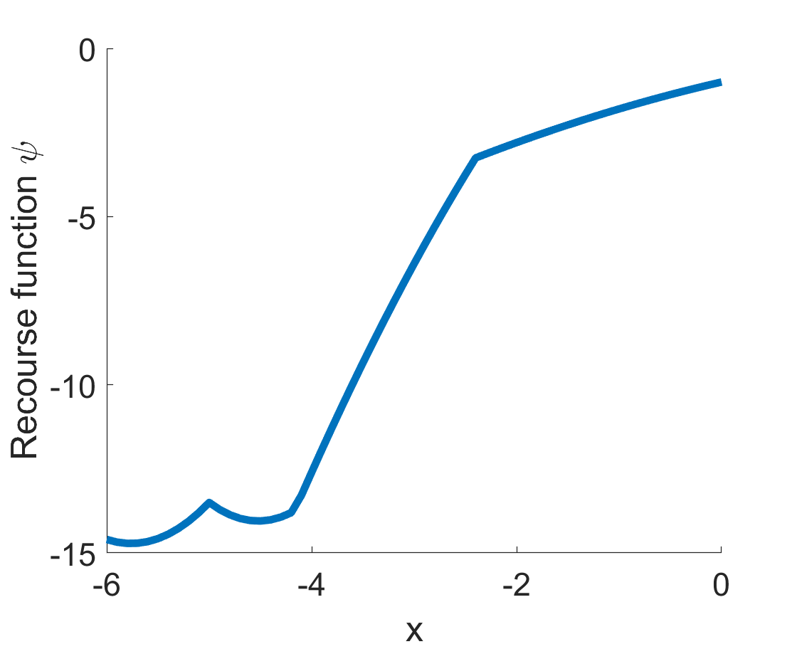
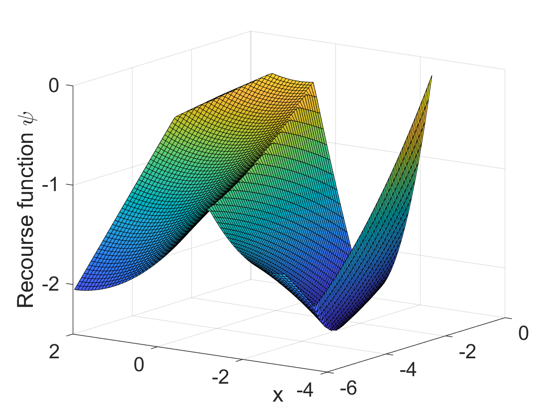
These two features together lead to a complex nonconvex and nonsmooth recourse function $\psi(\bullet;\xi)$ (see Figure 1 below), which constitutes the major challenge for designing rigorous and efficient numerical methods to solve problem (1).

Recourse functions in the form of (2) arise from many applications. One important source of the nonconvex recourse in (2) comes from the decision dependent/influenced uncertainty [30, 40, 34, 23], where the probability distribution $\mathbb{P}(x)$ of the random vector $\tilde{\xi}$ is dependent on the first-stage variable $x$. This is in contrast to the classical SP paradigm under exogenous uncertainty, where the distribution of $\tilde{\xi}$ is not affected by the first-stage decisions. There is growing interest in the endogenous uncertainty in recent literature of stochastic and robust programs [24, 25, 57, 30]. A typical example where the random parameters can be altered by a decision is that the price (as a first-stage variable) may affect the distribution of the product demand. Assume that the probability distribution of $\tilde{\xi}$ is given by $\mathbb{P}_{x}$ that depends on the first-stage variable $x$. We consider the corresponding two-stage SP model:

If there exists a decision-independent distribution $\widehat{\mathbb{P}}$ such that $\mathbb{P}_{x}$ is absolutely continuous with respect to $\widehat{\mathbb{P}}$ for any $x\in X$, we can reformulate the above problem by applying [22, Proposition 3.9] as:

where $\mbox{d}\mathbb{P}_{x}/\mbox{d}\widehat{\mathbb{P}}$ is the Radon-Nikodym derivative of $\mathbb{P}_{x}$ with respect to $\widehat{\mathbb{P}}$. Even if originally the first-stage decision $x$ only appears in the constrains of the second-stage problem in $\psi(x;\xi)$, the above transformation would make $x$ also appear in the second-stage objective function through the multiplication of $\mbox{d}\mathbb{P}_{x}/\mbox{d}\widehat{\mathbb{P}}$.

A specific example of the decision-dependent uncertainty in SPs is a power system planning problem originated in [36] and expanded in [30]. Assume that $\tilde{\xi}=(\{\tilde{d}_{j}\}_{j\in{\cal J}},\{\tilde{\pi}_{j}\}_{j\in{\cal J}},\{\tilde{q}_{i}\}_{i\in{\cal I}})$ follows a discrete distribution with the support $\{\xi^{s}\}_{s=1}^{S}$, where $\tilde{d}_{j}$ and $\tilde{\pi}_{j}$ represent the demand and the price of electricity in the location $j\in\mathcal{J}$, and $\tilde{q}_{i}$ is the unit production cost of the power plant $i\in\mathcal{I}$. For each $s=1,\cdots,S$, the probability of $\tilde{\xi}=\xi^{s}$ is the linear combination of $|\mathcal{G}|$ given different distributions (each with probability $p_{sg}$) whose weights $\{x_{g}\}_{g\in\mathcal{G}}$ are determined as parts of the first-stage decisions, i.e., $\mathbb{P}_{x}(\tilde{\xi}=\xi^{s})=\sum_{g\in\mathcal{G}}p_{sg}\,x_{g}$ for each $s$. The capacity of each power plant $\{x_{i}\}_{i\in\mathcal{I}}$ also needs to be determined in the first stage. The second-stage decisions are the production $y_{ij}$ from the power plant $i$ to the location $j$ for each $s$. By letting $\widehat{\mathbb{P}}(\tilde{\xi}=\xi^{s})=1/S$ for each $s$ in (3), we can rewrite the recourse function as

and obtain a decision-independent SP with the recourse $\widehat{\psi}$. Observe that both the objective and constraints depend on the first-stage variables. In particular, the objective function is convex in $x_{g}$ and concave in $y$, which fits our problem setting. Later, we will apply our proposed algorithms to solve a two-stage SP with the above recourse in Section 6.

The second example of the nonconvex recourse in (2) is the stochastic interdiction problem [18, 29], where the defender may want to maximize the second-stage objective function instead of minimizing it. Even for the simple linear second-stage problem with only $x$ appearing in the constraints, the recourse function

is not convex in $x$. One may take the dual of the second-stage maximization problem so that the recourse is a parametrized minimization problem

However, this dualization would bring a bilinear term $\lambda^{\top}T(\xi)x$ of the first-stage variable $x$ and the second-stage variable $\lambda$ to the objective function that necessities the concave-convex structure of $f(\bullet,\bullet;\xi)$. To the best of our knowledge, there is no known rigorous decomposition method to solve a general nonconvex two-stage min-max stochastic programs even under the linear setting.

When the distribution of $\tilde{\xi}$ is taken as the empirical distribution of observed realizations $\xi^{1},\ldots,\xi^{S}$, the simplest way to tackle the problem (1) is to simultaneously solve the first-stage variable $x$ and second-stage variables $y^{1},\ldots,y^{S}$ (each $y^{s}$ is associated with one scenario $\xi^{s}$) via the sample average approximation [55]:

However, this approach can be prohibitive when the number of scenarios $S$ is large since the dimension of the unknown variables is $n_{1}+n_{2}S$. Even if $S$ is small or moderate, the above formulation may still be difficult to handle under our setting as the function $f(\bullet,\bullet;\xi)$ is not jointly convex (for example when $f(\bullet,\bullet;\xi)$ is bilinear). In fact, the nonconvexity of the recourse function also makes it challenging to apply the stochastic approximation method [44, 43, 39] to solve (1), since it is not clear how to obtain a (Clarke) subdifferential of the nonconvex recourse function in (1). Without strong assumptions like the uniqueness of the second-stage solutions, only a superset of the subdifferential $\partial\psi(\bullet;\xi)$ at given $x$ is computable [10, Chapter 4]. When $f$ and $G$ are twice continuously differentiable, the authors in [11] have adopted a smoothing method to deal with the possibly nonconvex recourse by adding the Tikhonov-regularized barrier of the inequality constraints to the second-stage objective function. For a special class of two-stage nonconvex quadratic SPs under the simplex constraint, the paper [9] has derived upper and lower approximations of the objective values via copositive programs.

Notice that the constraints in (5) are in fact block-wise separable in $y^{1},\ldots,y^{S}$ so that there is a block-angular structure between the first- and second-stage variables. Decomposition algorithms of two-stage SPs take advantage of this special structure to efficiently handle a large number of scenarios via solving $S$ numbers of low-dimensional subproblems [52]. Two classical decomposition algorithms for two-stage SPs are (augmented) Lagrangian decomposition and Benders decomposition. (Augmented) Lagrangian decompositions (including the progressive hedging algorithm) copy the first-stage variable $S$ times and attach one to each scenario [26, 49]. In order to force the non-anticipativity of the first-stage decision, one has to add equality constraints among all copies to ensure that $x$ is the same across different realizations of the uncertainty. However, there are two major bottlenecks to apply such kind of dual-based algorithms to solve the problem (1). One, each subproblem pertaining to one pair of variables $(x^{s},y^{s})$ is still nonconvex if $f$ is not a jointly convex function, so that it is in general not easy to obtain its global optimal solution. Two, the convergence of these dual approaches is largely restricted to the convex problems or special integer problems [49, 14]. Although there are some recent advances for the convergence study of the progressive hedging algorithm for solving nonconvex SPs under the local convexity conditions [47, 48], it is not clear whether the problem (1) satisfies those conditions without further assumptions on $f$ and $g$. Benders decomposition (or L-shaped methods) [4, 58, 60] alternatively updates the first-stage and second-stage variables, where the second-stage subproblem can be solved in parallel to save the computational time and reduce storage burden. In order to derive valid inequalities of $x$ and add them to the first-stage master problem, one usually uses subgradient inequalities of the (convex) recourse function to generate a sequence of lower approximations. However, when the recourse function is associated with the complex nonconvex function in (1), it is challenging to derive its lower bounds based on the computed second-stage solutions. In fact, for the recourse functions in Figure 1, there seems not to exist a convex function that passes one of the downward cusps and at the same time approximates the original function from below.

In this paper, we tackle the two-stage stochastic programs (1) by a novel lifting technique that transforms the complex nonconvex and nondifferentiable recourse function (2) in the original space to a structured convex-concave function in a lifted space. The reveal of this latent structure enables us to construct convex surrogation of all recourse functions at the latest first-stage iterate, whose evaluations are decomposable across different scenarios. Such surrogate functions are then added to the master problem to generate the next first-stage iterate. We shall prove that repeating the above procedure, the sequence of the first-stage iterates converges to a properly defined stationary solution of (1). In order to further reduce the computational cost per step when the number of scenarios $S$ is large as well as to handle the case where $\tilde{\xi}$ is continuously distributed, we also propose a framework that incorporates sequential sampling into the surrogation algorithm. The sequential sampling method gradually adds scenarios and generates cuts along the iterations, which has the advantage that one may obtain satisfactory descent progress in the early iterations with relatively small sample sizes to accelerate the overall procedure.

The paper is organized as follows. Section 2 introduces notation and provides preliminary knowledge. In Section 3, we discuss the implicitly convex-concave structure of the recourse function and derive its computationally tractable approximations. A decomposition algorithm for solving problem (1) with a fixed number of scenarios is proposed and analyzed in Section 4. To further handle the continuously distributed random vectors as well as to reduce the computational cost of the decomposition algorithm in its early stage, we provide an internal sampling version of the algorithm in Section 5 and show the almost surely convergence of the iterative sequence. In Section 6, we conduct extensive numerical experiments to show the effectiveness of our proposed frameworks. The paper ends with a concluding section.

We first summarize the notation used throughout the paper. We write $\mathbb{Z}_{+}$ as the set of all nonnegative integers, and $\mathbb{R}^{n}$ as the $n$-dimensional Euclidean space equipped with the inner product $\langle x,y\rangle=x^{\top}y$ and the induced norm $\|x\|\triangleq\sqrt{x^{\top}x}$. The symbol $\mathbb{B}(x,\delta)$ is used to denote the closed ball of radius $\delta>0$ centered at a vector $x\in\mathbb{R}^{n}$. Let $A$ and $C$ be two nonempty subsets of $\mathbb{R}^{n}$. The diameter of $A$ is defined as $R(A)\triangleq\sup\limits_{x,y\in A}\|x-y\|$, and the distance from a vector $x\in\mathbb{R}^{n}$ to $A$ is defined as $\operatorname{dist}(x,A)\triangleq\inf\limits_{y\in A}\|y-x\|$. The one-sided deviation of $A$ from $C$ is defined as $\mathbb{D}(A,C)\,\triangleq\,\sup\limits_{x\in A}\operatorname{dist}(x,C)$.

We next introduce the concepts of generalized derivatives and subdifferentials for nonsmooth functions. Interested readers are referred to the monographs [16, 50, 38] for thorough discussions on these subjects. Consider a function $f:{\cal O}\rightarrow\mathbb{R}$ defined on an open set ${\cal O}\subseteq\mathbb{R}^{n}$. The classical one-sided directional derivative of $f$ at $\bar{x}\in{\cal O}$ along the direction $d\in\mathbb{R}^{n}$ is defined as $f^{\prime}(\bar{x};d)\,\triangleq\,\displaystyle\lim_{t\downarrow 0}\,\frac{f(\bar{x}+td)-f(\bar{x})}{t}$ if this limit exists. The function $f$ is said to be directionally differentiable at $\bar{x}\in{\cal O}$ if it is directionally differentiable along any direction $d\in\mathbb{R}^{n}$. In contrast, the Clarke directional derivative of $f$ at $\bar{x}\in{\cal O}$ along the direction $d\in\mathbb{R}^{n}$ is defined as $f^{\circ}(\bar{x};d)\,\triangleq\,\displaystyle\operatornamewithlimits{limsup}_{x\to\bar{x},\,t\downarrow 0}\,\frac{f(x+td)-f(x)}{t},$ which is finite when $f$ is Lipschitz continuous near $\bar{x}$. The Clarke subdifferential of $f$ at $\bar{x}$ is the set $\partial_{C}f(\bar{x})\triangleq\{v\in\mathbb{R}^{n}\mid f^{\circ}(\bar{x};d)\geq v^{\top}d\text{ for all $d\in\mathbb{R}^{n}$}\}$, which coincides with the usual subdifferential in convex analysis for a convex function. If $f$ is strictly differentiable at $\bar{x}$, then $\partial_{C}f(\bar{x})=\{\nabla f(\bar{x})\}$. We say that $f$ is Clarke regular at $\bar{x}\in{\cal O}$ if $f$ is directionally differentiable at $\bar{x}$ and $f^{\circ}(\bar{x};d)=f^{\prime}(\bar{x};d)$ for all $d\in\mathbb{R}^{n}$. This Clarke regularity at $\bar{x}$ is equivalent to have $f(x)\geq f(\bar{x})+\bar{v}^{\top}(x-\bar{x})+o(\|x-\bar{x}\|)$ for any $\bar{v}\in\partial_{C}f(\bar{x})$. Therefore, if a function fails to satisfy the Clarke regularity at $\bar{x}$ (for example at the downward cusp on the left panel of Figure 1), there does not exist an approximate linear lower bound of the original function based on the Clarke subdifferentials with small $o$ error locally.

Let $X\subseteq\mathbb{R}^{n}$ be a nonempty closed convex set and $f:\mathbb{R}^{n}\to\mathbb{R}$ be a locally Lipschitz continuous function that is directionally differentiable. We say $\bar{x}\in X$ is a directional-stationary point of $f$ on $X$ if $f^{\prime}(\bar{x};x-\bar{x})\geq 0$ for all $x\in X$, and a Clarke-stationary point if $f^{\circ}(\bar{x};x-\bar{x})\geq 0$ for all $x\in X$; the latter is equivalent to $0\in\partial_{C}f(\bar{x})+\mathcal{N}_{X}(\bar{x})$ with $\mathcal{N}_{X}(\bar{x})$ being the normal cone of $X$.

Let $\mathcal{F}:\mathbb{R}^{n}\,{\rightrightarrows}\,\mathbb{R}^{m}$ be a set-valued mapping. Its outer limit at $x\in\mathbb{R}^{n}$ is defined as

We say $\mathcal{F}$ is outer semicontinuous (osc) at $\bar{x}\in\mathbb{R}^{n}$ if $\limsup\limits_{x\rightarrow\bar{x}}\mathcal{F}(x)\subseteq\mathcal{F}(\bar{x})$.

A key ingredient to design a decomposition method for solving the two-stage SP (1) is to derive a computational-friendly approximation of the nonconvex recourse function (2) at any given $x\in X$ and $\xi\in\Xi$. This is the main content of the present section.

For simplicity, we omit $\xi$ in (2) throughout this section and rewrite the recourse function as, for $x\in\mathbb{R}^{n_{1}}$,

where $f(\bullet,\bullet)$ is concave-convex and $G(\bullet,\bullet)$ is jointly convex. We assume that for any $x\in\overline{X}$, the minimization problem of $y$ in (6) has an optimal solution, which implies the finiteness of $\psi(x)$ on $\overline{X}$. In the following, we show that the above function, although generally being nonconvex and nondifferentiable in $\mathbb{R}^{n_{1}}$, has a benign structure in a lifted space. Leveraging this structure, we then derive an approximate difference-of-convex decomposition of the recourse function that is computationally tractable. Such an approximation is the cornerstone of the decomposition methods to be presented in the next two sections.

Based on the discussion in the last section, we are now ready to present the decomposition algorithm for solving the nonconvex two-stage SP (1) and analyze its convergence. In this section, we focus on the case where there are fixed scenarios $\{\xi^{1},\ldots,\xi^{S}\}$, each realized with probability $1/S$. The problem (1) then reduces to

where each $\psi(x;\xi^{s})$ is given by (2). The above problem can be viewed as a sample average approximation of the two-stage SP (1) under a prescribed sample size $S$. All the discussions in this section can be easily adapted to the case where the distribution of $\tilde{\xi}$ has finite support (but unequal probability mass for different $\xi^{s}$). We will work on the internal sampling scheme for continuously distributed $\tilde{\xi}$ in the next section.

References

• [1] Le Thi Hoai An and Pham Dinh Tao. The DC (difference of convex functions) programming and DCA revisited with DC models of real world nonconvex optimization problems. Annals of Operations Research, 133(1-4):23–46, 2005.
• [2] Zvi Artstein and Richard A Vitale. A strong law of large numbers for random compact sets. The Annals of Probability, pages 879–882, 1975.
• [3] Edgar Asplund. Differentiability of the metric projection in finite-dimensional Euclidean space. Proceedings of the American Mathematical Society, 38(1):218–219, 1973.
• [4] Jacques F Benders. Partitioning procedures for solving mixed-variables programming problems. Numerische mathematik, 4(1):238–252, 1962.
• [5] Dimitri P Bertsekas. Control of uncertain systems with a set-membership description of the uncertainty. PhD thesis, Massachusetts Institute of Technology, 1971.
• [6] John R Birge and Francois Louveaux. Introduction to Stochastic Programming. Springer Science & Business Media, 2011.
• [7] Merve Bodur, Sanjeeb Dash, Oktay Günlük, and James Luedtke. Strengthened Benders cuts for stochastic integer programs with continuous recourse. INFORMS Journal on Computing, 29(1):77–91, 2017.
• [8] Natashia Boland, Jeffrey Christiansen, Brian Dandurand, Andrew Eberhard, Jeff Linderoth, James Luedtke, and Fabricio Oliveira. Combining progressive hedging with a Frank–Wolfe method to compute Lagrangian dual bounds in stochastic mixed-integer programming. SIAM Journal on Optimization, 28(2):1312–1336, 2018.
• [9] Immanuel M Bomze, Markus Gabl, Francesca Maggioni, and Georg Ch Pflug. Two-stage stochastic standard quadratic optimization. European Journal of Operational Research, 299(1):21–34, 2022.
• [10] J Frédéric Bonnans and Alexander Shapiro. Perturbation Analysis of Optimization Problems. Springer Science & Business Media, 2013.
• [11] Pedro Borges, Claudia Sagastizábal, and Mikhail Solodov. A regularized smoothing method for fully parameterized convex problems with applications to convex and nonconvex two-stage stochastic programming. Mathematical Programming, pages 1–33, 2020.
• [12] Richard H Byrd, Jorge Nocedal, and Richard A Waltz. Knitro: An integrated package for nonlinear optimization. In Large-scale nonlinear optimization, pages 35–59. Springer, 2006.
• [13] Claus C Carøe and Rüdiger Schultz. Dual decomposition in stochastic integer programming. Operations Research Letters, 24(1-2):37–45, 1999.
• [14] Bock Jin Chun and Stephen M Robinson. Scenario analysis via bundle decomposition. Annals of Operations Research, 56(1):39–63, 1995.
• [15] Frank H Clarke. Generalized gradients and applications. Transactions of the American Mathematical Society, 205:247–262, 1975.
• [16] Frank H Clarke. Optimization and Nonsmooth Analysis. SIAM, 1990.
• [17] Patrick L Combettes. Quasi-Fejérian analysis of some optimization algorithms. In Studies in Computational Mathematics, volume 8, pages 115–152. Elsevier, 2001.
• [18] Kelly J Cormican, David P Morton, and R Kevin Wood. Stochastic network interdiction. Operations Research, 46(2):184–197, 1998.
• [19] Ying Cui and Jong-Shi Pang. Modern Nonconvex Nondifferentiable Optimization. SIAM, 2021.
• [20] John M Danskin. The theory of max-min and its application to weapons allocation problems, volume 5. Springer Science & Business Media, 2012.
• [21] Yuri M Ermoliev and Vladimir I Norkin. Sample average approximation method for compound stochastic optimization problems. SIAM Journal on Optimization, 23(4):2231–2263, 2013.
• [22] Gerald B Folland. Real analysis: modern techniques and their applications, volume 40. John Wiley & Sons, 1999.
• [23] Vikas Goel and Ignacio E Grossmann. A stochastic programming approach to planning of offshore gas field developments under uncertainty in reserves. Computers & Chemical Engineering, 28(8):1409–1429, 2004.
• [24] Vikas Goel and Ignacio E Grossmann. A Lagrangian duality based branch and bound for solving linear stochastic programs with decision dependent uncertainty. In Computer Aided Chemical Engineering, volume 20, pages 55–60. Elsevier, 2005.
• [25] Vikas Goel and Ignacio E Grossmann. A class of stochastic programs with decision dependent uncertainty. Mathematical Programming, 108(2):355–394, 2006.
• [26] Monique Guignard. Lagrangean relaxation. Top, 11(2):151–200, 2003.
• [27] Vincent Guigues. Inexact stochastic mirror descent for two-stage nonlinear stochastic programs. Mathematical Programming, 187(1):533–577, 2021.
• [28] Vincent Guigues, Renato Monteiro, and Benar Svaiter. Inexact cuts in stochastic dual dynamic programming applied to multistage stochastic nondifferentiable problems. SIAM Journal on Optimization, 31(3):2084–2110, 2021.
• [29] Tianyu Hao and Jong-Shi Pang. Piecewise affine parameterized value-function based bilevel non-cooperative games. Mathematical Programming, 180(1):33–73, 2020.
• [30] Lars Hellemo, Paul I Barton, and Asgeir Tomasgard. Decision-dependent probabilities in stochastic programs with recourse. Computational Management Science, 15(3):369–395, 2018.
• [31] Julia L Higle and Suvrajeet Sen. Stochastic decomposition: a statistical method for large scale stochastic linear programming, volume 8. Springer Science & Business Media, 2013.
• [32] Tito Homem-de Mello. Variable-sample methods for stochastic optimization. ACM Transactions on Modeling and Computer Simulation, 13(2):10–133, 2003.
• [33] Tito Homem-de Mello and Güzin Bayraksan. Monte Carlo sampling-based methods for stochastic optimization. Surveys in Operations Research and Management Science, 19(1):56–85, 2014.
• [34] Tore W Jonsbråten, Roger J.-B. Wets, and David L Woodruff. A class of stochastic programs with decision dependent random elements. Annals of Operations Research, 82:83–106, 1998.
• [35] Junyi Liu, Ying Cui, Jong-Shi Pang, and Suvrajeet Sen. Two-stage stochastic programming with linearly bi-parameterized quadratic recourse. SIAM Journal on Optimization, 30(3):2530–2558, 2020.
• [36] François V Louveaux. Optimal investments for electricity generateion: A stochastic model and a test problem. Numerical Techniques for Stochastic Optimization, 1988.
• [37] Yves Lucet. Fast Moreau envelope computation I: Numerical algorithms. Numerical Algorithms, 43(3):235–249, 2006.
• [38] Boris S Mordukhovich. Variational Analysis and Generalized Differentiation I: Basic Theory, volume 330. Springer Science & Business Media, 2006.
• [39] Arkadi Nemirovski, Anatoli Juditsky, Guanghui Lan, and Alexander Shapiro. Robust stochastic approximation approach to stochastic programming. SIAM Journal on Optimization, 19(4):1574–1609, 2009.
• [40] Omid Nohadani and Kartikey Sharma. Optimization under decision-dependent uncertainty. SIAM Journal on Optimization, 28(2):1773–1795, 2018.
• [41] Raghu Pasupathy and Yongjia Song. Adaptive sequential sample average approximation for solving two-stage stochastic linear programs. SIAM Journal on Optimization, 31(1):1017–1048, 2021.
• [42] Chayne Planiden and Xianfu Wang. Proximal mappings and Moreau envelopes of single-variable convex piecewise cubic functions and multivariable gauge functions. In Nonsmooth optimization and its applications, pages 89–130. Springer, 2019.
• [43] Boris T Polyak. New stochastic approximation type procedures. Automat. i Telemekh, 7(98-107):2, 1990.
• [44] Herbert Robbins and Sutton Monro. A stochastic approximation method. The annals of mathematical statistics, pages 400–407, 1951.
• [45] Herbert Robbins and David Siegmund. A convergence theorem for nonnegative almost supermartingales and some applications. In Optimizing Methods in Statistics, pages 233–257. Elsevier, 1971.
• [46] R Tyrrell Rockafellar. Convex analysis, volume 18. Princeton university press, 1970.
• [47] R Tyrrell Rockafellar. Progressive decoupling of linkages in optimization and variational inequalities with elicitable convexity or monotonicity. Set-Valued and Variational Analysis, 27(4):863–893, 2019.
• [48] R Tyrrell Rockafellar. Augmented Lagrangians and hidden convexity in sufficient conditions for local optimality. Mathematical Programming, 192, 2022.
• [49] R Tyrrell Rockafellar and Roger J-B Wets. Scenarios and policy aggregation in optimization under uncertainty. Mathematics of Operations Research, 16(1):119–147, 1991.
• [50] R Tyrrell Rockafellar and Roger J-B Wets. Variational Analysis, volume 317. Springer Science & Business Media, 2009.
• [51] Johannes Royset and Elijah Polak. Extensions of stochastic optimization results to problems with system failure probability functions. Journal of Optimization Theory Applications, 133:1–18, 2007.
• [52] Andrzej Ruszczyński. Decomposition methods in stochastic programming. Mathematical Programming, 79(1-3):333–353, 1997.
• [53] Rüdiger Schultz. Stochastic programming with integer variables. Mathematical Programming, 97(1):285–309, 2003.
• [54] Alexander Shapiro. Monte Carlo sampling methods. Handbooks in Operations Research and Management Science, 10:353–425, 2003.
• [55] Alexander Shapiro, Darinka Dentcheva, and Andrzej Ruszczyński. Lectures on Stochastic Programming: Modeling and Theory. SIAM, 2021.
• [56] Alexander Shapiro and Huifu Xu. Uniform laws of large numbers for set-valued mappings and subdifferentials of random functions. Journal of Mathematical Analysis and Applications, 325(2):1390–1399, 2007.
• [57] Bora Tarhan, Ignacio E Grossmann, and Vikas Goel. Stochastic programming approach for the planning of offshore oil or gas field infrastructure under decision-dependent uncertainty. Industrial & Engineering Chemistry Research, 48(6):3078–3097, 2009.
• [58] Richard M Van Slyke and R. J.-B. Wets. L-shaped linear programs with applications to optimal control and stochastic programming. SIAM Journal on Applied Mathematics, 17(4):638–663, 1969.
• [59] Andreas Wächter and Lorenz T Biegler. On the implementation of an interior-point filter line-search algorithm for large-scale nonlinear programming. Mathematical Programming, 106(1):25–57, 2006.
• [60] R. J.-B. Wets. Large scale linear programming techniques in stochastic programming. IIASA Working Paper, 1984.