Naturally embedded in the CV model are quantum gates to directly implement the expression $L(\ket{x})=\ket{\phi(Wx+b)}$.

The affine transformation $Wx+b$ is implemented by the composition $\mathit{D}\circ\mathit{U}_{2}\circ\mathit{S}\circ\mathit{U}_{1}$, where $U_{k}$ denotes the $k^{th}$ interferometer, $S$ a set of $m$ squeezers, $D$ a set of $m$ displacement gates. The activation function $\phi(\ket{\cdot})$ is implemented by a set of Kerr gates, which are non-linear. The composition $\phi\circ\mathit{D}\circ\mathit{U}_{2}\circ\mathit{S}\circ\mathit{U}_{1}$ acting on a quantum state $\ket{x}$ gives us the desired state $L(\ket{x})=\ket{\phi(Wx+b)}$. The schematic of the circuit is shown below.

The interferometer $U_{k}$ on an $m-$qumode system is composed of $m-1$ beamsplitters and $m$ rotation gates as shown in the figure.

The action of a phaseless interferometer $\mathit{U}_{k}$ on the quantum state $\ket{x}=\otimes_{k=1}^{m}\ket{x_{k}}$ has an effect of an orthogonal matrix acting on $\ket{x}$ [cv_19]. Orthogonal matrices are just unitary matrices with real entries, inducing length-preserving rotations. Then the transpose of an orthogonal matrix represents the reverse rotation of the original matrix, thus orthogonal. Then the composition $U_{2}\circ S\circ U_{1}$ can be considered as the composition $O_{2}\circ S\circ\left(O_{1}^{T}\right)^{T}$, where $O_{2}$ and $O_{1}^{T}$ are orthogonal.

Let $W$ be the linear transformation matrix we want to implement with a quantum circuit. Any matrix $W$ can be factorized using singular value decomposition (SVD) as $W=U\Sigma V^{\ast}$, where $U$ and $V$ are orthogonal and $\Sigma$ is diagonal [SVD]. The parameterized squeezer $S(r_{k})$ acts on the quantum state $\ket{x_{k}}$ of each $k^{th}$ qumode as $S(r_{k})\ket{x_{k}}=\sqrt{e^{-r_{k}}}\ket{e^{-r_{k}}x_{k}}$. Collectively they have an effect of a diagonal matrix $\mathit{S}=S(r_{1})\otimes S(r_{1})\otimes\ldots\otimes S(r_{m})$ acting on $\ket{x}=\otimes_{i=1}^{m}\ket{x_{k}}$. The composition $\mathit{U}_{2}\circ\mathit{S}\circ\mathit{U}_{1}$ implements a quantum version of the linear transformation matrix $W$ [cv_19].

The bias addition is realized with displacement gates $D$. The displacement gate has an effect

$$D(\alpha_{k})\ket{\psi_{k}}=\ket{\psi_{k}+\sqrt{2}\alpha_{k}}$$

for each $k^{th}$ qumode. Then $D(\alpha)\ket{\psi}=\ket{\psi+\sqrt{2}\alpha}$ collectively for $\alpha^{T}=[\alpha_{1},\alpha_{2},\ldots,\alpha_{m}]$. For some desired bias $b$, let $\alpha=\frac{b}{\sqrt{2}}$, then the collection of displacement gates implements the bias addition. The composition $D\circ U_{2}\circ S\circ U_{1}$ acting on the quantum state $\ket{x}$ gives us the affine transformation

$$D\circ U_{2}\circ S\circ U_{1}\ket{x}=\ket{O_{2}\Sigma O_{1}x+b}=\ket{Wx+b}.$$

The non-linear activation function $\phi(\cdot)$ is realized with Kerr gates. The Kerr gate, parameterized by the parameter $\kappa$, is a non-linear transformation gate. Let $n$ be the cutoff dimension and $m$ the number of qumodes. For the quantum state $\ket{\psi}$ of one qumode, which is a superposition of $n$ Fock basis states, the Kerr gate with parameter $\kappa$ has an effect

$$\aligned K(\kappa)\ket{\psi}&=\bmatrix e^{i\kappa 0^{2}}0\ldots 0\\ 0e^{i\kappa 1^{2}}\ldots 0\\ \vdots\ddots\vdots\\ 00\ldots e^{i\kappa(n-1)^{2}}\\ \bmatrix\psi_{0}\\ \psi_{1}\\ \vdots\\ \psi_{n-1}\\ \\ =\bmatrix\psi_{0}\\ e^{i\kappa 1^{2}}\psi_{1}\\ \vdots\\ e^{i\kappa(n-1)^{2}}\psi_{n-1}\\ ,$$

which is non-linear.

Together, the circuit $L=\Phi\circ D\circ U_{2}\circ S\circ U_{1}$ gives us a quantum version $L\left(\ket{x}\right)=\ket{\Phi(Wx+b)}$ of a classical neural network $L(x)=\Phi(Wx+b)$.

The binary classifier outlined in ”Continuous-variable quantum neural networks” is a classical and quantum hybrid network [cv_19].

The dataset used contains 284,806 genuine and fraudulent credit card transactions with 29 features, out of which only 492 are fraudulent. The dataset is truncated to 10 features as per the paper and 1,968 samples with 1:3 ratio of fraudulent vs. genuine.

The proposed classical-quantum hybrid model has a classical neural network taking input vectors of size 10 and outputting vectors of size 14, quantum encoding circuit, and a 2-qumode quantum neural network which outputs vectors of size 2. We can regard the output vectors as one-hot encoding of binary classification of fraudulent vs. genuine. The architecture of the hybrid network is

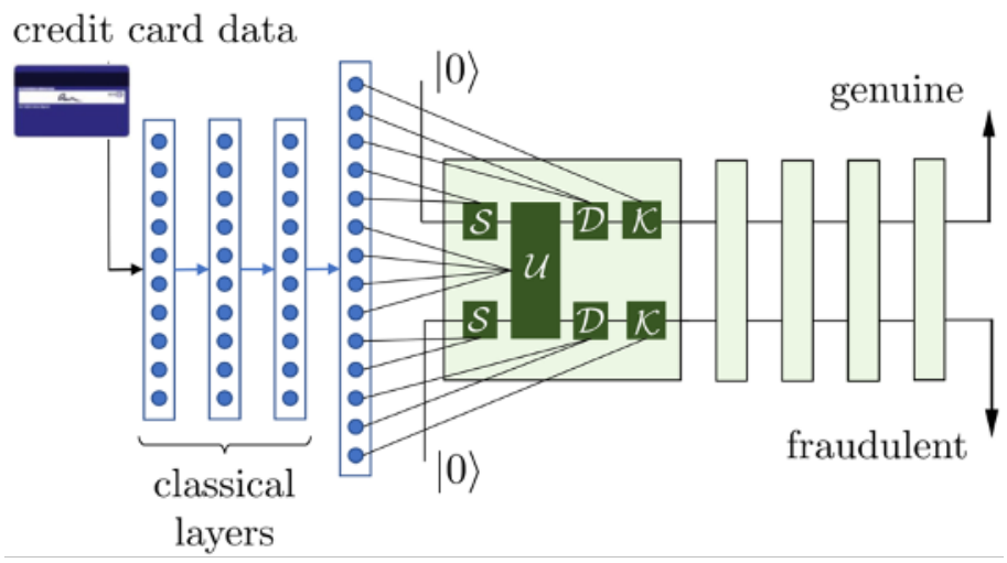
The data flow of the circuit is

• •

  Classical network: 2 hidden layers with 10 neurons, each using Exponential Linear Units (ELU) as activation function. Output layer with 14 neurons.

• •

  Data encoding: Output vector from the classical network is converted to a quantum state by the circuit - squeezers, interferometer, displacement gates, and Kerr gates

• •

  Quantum network: 4 layers of QNN. Each layer is composed of interferometer 1, squeezers, interferometer 2, displacment gates, and Kerr gates.

• •

  Measurement: The expectation value of the Pauli$-X$ gate $\bra{\phi_{k}}X\ket{\phi_{k}}$ is evaluated for each qumode state$\ket{\phi_{k}}$ for the $k^{th}$ qumode.

The experiment yields $97\%$ training accuracy.

\href

https://github.com/sophchoe/Binary_Classification_Pennylane_KerasCode: Keras-Pennylane implementation