Near infrared and optical emission of WASP-5 b
Abstract
Context. Thermal emission from extrasolar planets makes it possible to study important physical processes in their atmospheres and derive more precise orbital elements.
Aims. By using new near infrared and optical data, we examine how these data constrain the orbital eccentricity and the thermal properties of the planet atmosphere.
Methods. The full light curves acquired by the TESS satellite from two sectors are used to put upper limit on the amplitude of the planet’s phase variation and estimate the occultation depth. Two, already published and one, yet unpublished followup observations in the 2MASS K (Ks) band are employed to derive a more precise occultation light curve in this near infrared waveband.
Results. The merged occultation light curve in the Ks band comprises data points. The data confirm the results of the earlier eccentricity estimates, suggesting circular orbit: . The high value of the flux depression of ppt in the Ks band excludes simple black body emission at the level and disagrees also with current atmospheric models at the level. From the analysis of the TESS data, in the visual band we found tentative evidence for a near noise level detection of the secondary eclipse, and placed constraints on the associated amplitude of the planet’s phase variation. A formal box fit yields an occultation depth of ppt. This implies a relatively high geometric albedo of for fully efficient atmospheric circulation and for no circulation at all. No preference can be seen either for the oxygen-enhanced, or for the carbon-enhanced atmosphere models.
Key Words.
Planets and satellites: atmospheres – Methods: data analysis1 Introduction
The year 2005 marks the first direct detection of the light radiated by an extrasolar planet (Charbonneau et al. 2005; Deming et al. 2005). The observations were made by the Spitzer space telescope (Werner et al. 2004) at , and , not easily accessible by ground-based instruments. Although it was quite expectable that a similar measurement in the near infrared could also be possible by ground-based -class telescopes, two years passed until the first tentative observation of that kind (Snellen & Covino 2007). Since then, secondary eclipse (occultation) observations at the (2MASS K – or Ks) band still remained in the realm of ground-based instruments, due to the lack of space instruments at this wavelength (Croll 2015; Zhou et al. 2015; Martioli et al. 2019, e.g.,). The 2MASS bands are especially suitable for the observation of hot extrasolar planets, due to the expected peaking of the black-body flux in for temperatures between and K, i.e., for the characteristic equilibrium temperatures of extrasolar planets (Alonso 2018, e.g., ).
Here we revisit WASP-5, an “ordinary” extrasolar planetary system, discovered by the SuperWASP collaboration (Anderson et al. 2008). The system harbors a single planet with a main sequence host, akin to our Sun. So far, no other planets have been reported in the system, although there are contradictory results concerning the origin of the transit time variation of planet b (Fukui et al. 2011; Hoyer et al. 2012, i.e., ). Based on the followup work of Gillon et al. 2009, the main system parameters are as follows: , , K, AU, , . These parameters imply an equilibrium temperature (assuming zero albedo and full heat redistribution) of K (Chen et al. 2014). The orbital period is d, derived in this paper from the combination of the earlier epochs and those resulting from the analysis of the data from the TESS satellite (Ricker et al. 2015).
Occultation observations in the Ks band have already been carried out by Chen et al. 2014 and Zhou et al. 2015. Here, we combine these data with our unpublished observations made by the -m Walter Baade Telescope at the Las Campanas Observatory.11 1 The Ks band photometric time series used in this paper are available at the CDS via anonymous ftp to cdsarc.u-strasbg.fr (130.79.128.5) or via http://cdsarc.u-strasbg.fr/viz-bin/qcat?J/A+A/3digitVol/Apagenumber
Our main goal is to increase the precision of the estimation of the occultation depth – an important ingredient for a more reliable model fitting, as most of the observations (including ours) sample the planetary spectra only in few, isolated bands. To constrain the atmosphere further, we utilize the recent data collected by the TESS satellite. We search for reflected light variation and occultation event. As a by-product of our analysis, we search also for additional planets (and find none).
2 Datasets
Two occultation light curves in the near infrared Ks-band have been published so far on WASP-5 b. Chen et al. 2014 used the MPG/ESO m telescope to observe the target in all three 2MASS bands. In spite of the substantial instrumental systematics they clearly detected the event after applying corrections due to positional and image quality dependences. Zhou et al. 2015 performed a survey of seven hot Jupiters by using the Anglo-Australian Telescope (AAT). Their survey included also WASP-5, yielding a long-stretched coverage, allowing sufficient baseline in the eclipse modeling. Details of the observational settings and the methods used are described in the corresponding papers.
| Set | Date [UT] | Dur. [h] | N | Exp. [s] | Observer | Ref. | Instr. / Telescope / Site |
|---|---|---|---|---|---|---|---|
| 1 | 08-09-2011 | 4.60 | 699 | Chen∙ | Chen et al. 2014 | GROND / MPG / ESO 2.2 / La Silla (Chile) | |
| 2 | 09-11-2011 | 4.33 | 2084 | Dékány⋆ | this paper | FourStar / Baade 6.5 / Las Campanas (Chile) | |
| 3 | 14-09-2014 | 5.99 | 1732 | Zhou | Zhou et al. 2015 | IRIS2 / AAT 3.9 / Siding Spring (Australia) |
Notes: All data were taken in the 2MASS K color, except for set-1, where the custom made K filter of the GROND instrument was used (with a transmission curve very close to that of the 2MASS K band). ∙Technical assistance is provided by Timo Anguita (Chen et al. 2014, see ). ⋆Assisted by Markus Rabus. ▲Typical integration time.
The third dataset comes from our single-night observations on 9 November, 2011 (UT). The four-chip camera of the FourStar infrared imager attached to the -m Walter Baade telescope was used to gather high cadence Ks images on the field hosting WASP-5. An integration time of s was used, yielding a s overall sampling interval. For better photometric accuracy, the telescope was slightly defocused, resulting in stellar images of diameter. All images were taken in a simple staring mode, without dithering. Unfortunately, the sky was not photometric throughout the night, due to intermittent clouds. This has led to losing some data points primarily after the ingress, affecting % of the full observing run.


To obtain the photometric fluxes, we employed both the classical iraf22 2 iraf is distributed by the National Optical Astronomy Observatories, which are operated by the Association of Universities for Research in Astronomy, Inc., under cooperative agreement with the National Science Foundation. routines and those of the fitsh33 3 https://fitsh.net/ package by Pál 2012. The two methods have led to very similar results, so we decided to use our earlier reduction made by iraf.
First we performed the standard reduction steps of bias, dark and flat corrections, including a treatment for the overall infrared sky emissivity variation by a nonlinear iterative multistep method, the nebulosity filtering algorithm44 4 http://casu.ast.cam.ac.uk/publications/nebulosity-filter/nebulosity_filter.pdf of Irwin 2010. Then, we tested several aperture sizes to select the one that yielded the least scatter in the corresponding ensemble light curves (LCs). It turned out that nearly all apertures yield the same quality LCs, with a slight preference toward the mid-sized apertures. Finally, we selected the one with the aperture radius of pixels (), outer annulus starting at pixel radius of and ending at , to assess the temporal background level.
In deriving the final ensemble LC (i.e., the target flux divided by the simple sum of the fluxes of the comparison stars), we decided not to use any comparison star from chips others than chip 1, that hosts the target. On this chip, (see Fig. 1) we have two bright comparison stars (No. 2 and 3) and a fainter one (No. 4). We found that adding the fainter star slightly increases the noise55 5 This is because the noise is not Poissonian. For faint objects, important contribution comes from the atmosphere, that acts on the derived fluxes of faint stars more violently, due to the increased significance of the background noise., therefore, we settled with the ensemble of the two brightest stars only.
3 Merging the three Ks light curves
Before some of the peculiarities of the merging process are detailed, we describe the steps leading to the ensemble LC of the FourStar/Baade data (set-2 in Table 1).
3.1 The FourStar/Baade light curve
As mentioned, the biggest issue with the data is the temporal cloudiness during some part of the first half of the observation. The top three panels of Fig. 2 show the flux variation for the entire run, including the target and the two comparison stars. It is worth noting that for the better visibility of the part of the flux variation that is dominated by the non-outlying points, we limited the plots at the % flux drop. Several data points reach as much as –% drops.

Although the comparison stars serve an excellent diagnosis on the environmental origin of the harsh variations seen in the target, and the ensemble flux ratio cures most of the variation, we see in the bottom panel that the large drops in the flux could not be filtered out at the level required by the small signal we are searching for. Nevertheless, the binned LC strongly suggests the presence of an underlying occultation signal. We note that in constructing the binned LC, we used overlapping bin sets with a shift of half of the bin width. In this way we can test the dependence of the binned LC on the bin distribution, which is an important piece of information on the sensitivity of any conclusion to be drawn from the binned LC – even if the conclusion is only preliminary.
In processing further the set-2 data, we observe the following: 1) there are outlier data points that are concentrated in a sufficiently broad section of the full time series and, therefore, might seriously bias the derived eclipse parameters; 2) likely because of (however small) differential extinction, there is a significant downward trend in the ensemble LC. This should also be filtered out. 3) A closer inspection of the ensemble LC in the bottom panel of Fig. 2 reveals that roughly in the middle of the cloudy period the flux suddenly jumped by a small fraction, enough to make a visible effect on the expected shallow eclipse. The most likely cause of this jump is the short-time change in the telescope pointing, leading to a sudden variation in the ensemble of pixels used in the flux evaluation. Leaving this jump in the ensemble LC would bias the occultation depth.

By following the principle of ‘least data massaging’, we proceeded as follows. For the treatment of outliers (issue 1) we robustly fitted66 6 In the standard least squares fit we employed Cauchy weights, adjusted iteratively to the processed time series – see, e.g., Kovacs 2020. -order polynomials to the fluxes of the target and the comparison stars. After the fit we employed a -clipping for the outliers and replaced these items by the corresponding polynomial values for the respective fluxes. In this way we naturally ended up with an ensemble LC that had no outliers, however, showed some trace of the ‘trimming’ made. Figure 3 displays where the polynomial replacement of the original data points were made (green dots). When both the target and all of the comparison stars had to be corrected, we see a continuous sequence of points. In all other cases the corrected points scatter around the ridge, represented by the binned LC (yellow points).
The linear trend and the jump in the ensemble LC (issues 2 and 3) were treated within an iterative process by filtering out these systematics, fitting the cleaned LC to an eclipse model and then subtracting this eclipse model from the starting dataset to get the next approximation for the systematics.
The systematics were represented by a linear function for the trend and a jump function to handle the discontinuity mentioned above:
| (1) |
where is the observed flux, is the time, measured from the first data point. is the Heaviside function with unit step at d. The jump position was fixed throughout the fit. Because the star blocks all radiation from the planet, the trapezoidal approximation for the occultation light curve suits perfectly:
| (2) | |||
| (3) | |||
| (4) | |||
| (5) |
, wheret_1,t_2,t_3t_4t_2-t_1 = t_4-t_3 = Δtδ{t_i}{c_i}
3.2 The three light curves
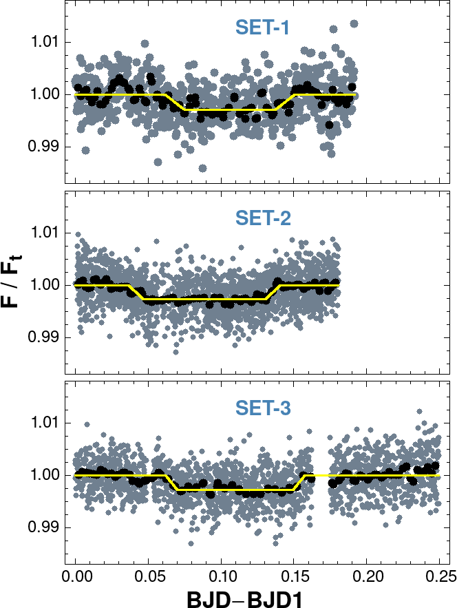
In trying to treat all three datasets in the same way, i.e., by starting from the simple ensemble light curve and employing the “minimum massage” post processing step, we found that the case of set-1 (Chen et al. 2014) is different. Since the ensemble light curve suffers excessively from systematics (see Fig. 2 of that paper), we decided to use their processed light curve that was obtained by applying carefully chosen external parameters (such as stellar position and image size) to separate systematics. On the other hand, for set-3 of Zhou et al. 2015 we used their simple ensemble light curve, even though there is also a substantial nonlinear trend in the data. In spite of this, we decided not to use an airmass or some polynomial correction (as given in the original paper), since this may introduce unpredictable changes in the eclipse and significantly depress the depth of the occultation.
All three light curves (sets-1 and -3 as above, set-2 as given in Fig. 3) serve as the input time series to fit them individually by the eclipse model and a linear trend (extended by a jump function for set-2). The result of this procedure is shown in Fig. 4.
3.3 Merging the three light curves
Before constructing the merged light curve, we need to check if such a merging is possible, i.e., if there is a unique orbital period that matches all three light curves within the observational errors. Evaluation of the updated orbital period by using the primary transit observations from the TESS satellite and combining the ephemerides with earlier followup data will be given in Sect. 4. Here we merely use the orbital period and the moment of the transit derived from that analysis.


By fitting the individual folded light curves we can examine if the data suggest strong discrepancies signaling warnings to be considered during the merging process. Figure 5 shows the individual phase-folded fits, indicating that the three datasets are in reasonable agreement, even if we consider set-1, the most discrepant from all. Set-1 contains the least number of data points ( vs and for set-2 and 3, respectively), and has also the largest residual (data minus fit) scatter (in relative flux units: , vs and ). In spite of these differences, all three datasets yield remarkably close egress phases. The cause of this is not entirely clear at this moment. In some cases, it might be simply the sign of more stable sky conditions in the second part of the run (i.e., for set-2 this was indeed the case).
In the final step of the merging process, we packed all data points in a single phase-folded dataset, by discarding the relatively small differences in data quality (i.e., weighting all data points from all sets equally).77 7 This choice is partially justified, because of the compensating effect of the larger number of points for the datasets with somewhat lower noise. The phase-folded light curve, containing all the data points, was robustly fitted by the trapezoidal model. The resulting binned light curve and the best-fit trapezoidal are shown in Fig. 6. The fitted parameters are listed in Table 2. The errors were computed from simple Monte Carlo simulations, whereby the binned light curve (mapped back to all the phase points) was perturbed by a bin-dependent Gaussian noise. We opted to use the binned time series rather than the trapezoidal fit, because of the remaining systematics, especially before/after the ingress/egress. We generated mock time series, fitted trapezoidals to each realization, and, after completion, we computed the standard deviations of the parameters. We refer to these standard deviations as the errors of the respective parameters. In Appendix A we give further details of the error calculation and the improvement of the parameters by using the merged data as compared with the fits to the individual datasets.
| Parameter | Value | Error |
|---|---|---|
| 0.47146 | 0.00219 | |
| 0.53102 | 0.00139 | |
| 0.05956 | 0.00270 | |
| 0.00528 | 0.00070 | |
| 0.00270 | 0.00014 |
Notes: All eclipse times are in the units of the orbital phase. Eclipse depth is the relative flux depression. The ingress and egress times, and can be converted into Barycentric Julian Date (TDB standard) by using the following formulae, e.g., for the ingress: [BJD], where is the epoch number of the event of interest and is the moment of the transit center and d is the orbital period. Epochs are ‘as observed’, i.e., no correction was made due to orbital light time effect of s.
4 Analysis of the TESS data
We use the light curves acquired by the full sky survey satellite TESS for: a) updating the ephemeris of the transit (since the occultation and the transit data were acquired in different epochs, we need a precise ephemeris to predict the transit phase right before the occultation occurred, if we want to make an estimation on the eccentricity); b) to measure the emission in the optical, we need space-based data, because of the high precision needed to detect the signature of the planet at this wavelength in the phase of occultation – the thermal emission in the optical is small, due to the planet’s low temperature and, in general, the albedos of the gas giants are also small (Wong et al. 2020; Wong et al. 2021, e.g.,).
WASP-5 was observed by TESS in sector between August 22 and September 20, 2018. Then, the object was revisited while scanning sector between August 26 and September 22, 2020. The two segments comprise altogether over data points in the short cadence ( min) sampling rate. We note that Wong et al. 2020 have already performed an analysis of the sector data and ended up with similar conclusions to ours as to be detailed in the subsections below.
Figure 7 shows the light curves from the above two sectors after employing the Presearch Data Conditioning (PDC) method of Smith et al. 2012 and Stumpe et al. 2012 implemented in the TESS pipeline88 8 See the corresponding TESS manual https://heasarc.gsfc.nasa.gov/docs/tess/docs/jenkinsSPIE2016-copyright.pdf. The Simple Aperture Photometric (SAP) time series served as the input for the PDC filter. Both types of data were downloaded from the STScI MAST site.99 9 https://archive.stsci.edu/hlsp/search.php We filtered the data further by using a -order robust polynomial fit to minimize the effect of the remaining systematics and possible stellar variability. The effect of this filtering is discussed in Appendix B.
Because sector SAP data suffer from a large number of outlying data points, to make the analysis uniform, we performed an iterative clipping for all datasets. The clipping was made relative to the transit model and the clipped values were set equal to the corresponding model values.

4.1 Updating transit ephemeris
To derive transit light curves free from other variations, we employed the same type of robust iterative method as briefly described in Sect. 3.1. The input data were the PDC/SAP time series as mentioned above. The model time series constituted two multiplicative parts: the transit and a -order polynomial. For the transit we adopted the simple model of Kovacs 2020, representing the ingress/egress phases as linear flux depressions with the same steepness and duration. The limb darkening was modeled by a scalable U-shaped function. We found this model quite satisfactory at the level of the accuracy of the data analyzed.
| Sect. | Type | [] | [d] | [d] | [flux] |
|---|---|---|---|---|---|
| 02 | SAP | 2458355.50802 | 0.09870 | 0.01091 | 0.01335 |
| 02 | PDC | 2458355.50807 | 0.09855 | 0.01083 | 0.01340 |
| 29 | SAP | 2459088.30168 | 0.09781 | 0.01082 | 0.01382 |
| 29 | PDC | 2459088.30166 | 0.09673 | 0.01017 | 0.01380 |
The transit parameters for the various time series are shown in Table 3. After combining these with the transit parameters obtained from the five followup observations of Baluev et al. 2019, Moyano et al. 2017, Hoyer et al. 2012, Fukui et al. 2011 and Anderson et al. 2008, we found that the orbital period of Fukui et al. 2011 should be decreased by s to properly match the published epochs.1010 10 When using the period of Fukui et al. 2011 we get an overall difference of min, whereas with the s lower period the differences are below min and mostly min. By choosing sector timing as a reference, the final ephemeris is given in Table 4. The error of the epoch was computed from simple Monte Carlo simulations by using the PDC data and is equal to the standard deviation of the epochs obtained from the realizations. The error on the period was calculated from , where d as given in Fukui et al. 2011, is the epoch error as given in Table 4 and the integer in the denominator is the elapsed epoch number between the two epochs. It is worth noting that the currently published ephemerides by Ivshina & Winn 2022 are in complete agreement with ours. There are ms and s differences between the periods and transit centers, respectively, corresponding an agreement within .
| [] | |
|---|---|
Notes: resulted from the analysis of the current (2018 and 2020) TESS visits, the period was derived from the combination of these TESS data and earlier followup observations dated back to the discovery (Anderson et al. 2008) of WASP-5.
4.2 Search for occultation and phase variation
To test the dependence of a possible detection of these delicate features on the data processing methods, we used four data types: SAP light curve with or without robust polynomial correction (see Sect. 4.1); PDC light curve with the same options. After prewhitening by the transit, we performed a bin signal search in the light curve folded by the orbital period. To account for the possible other variations, we employed a fully binned analysis, where the out of eclipse region was also divided into bins of the same size as the eclipse duration. After the bin with the largest flux depression was identified, we used a simple statistic to characterize its significance. Similarly, the phase variation was studied simply by a single-component Fourier fit to the original (i.e., not binned) phase-folded light curve. Significance tests were performed by using injected signals into pure Gaussian time series. Further details on the secondary eclipse and phase variation searches together with the supplementary statistical tests are given in Appendix B. Here we summarize the constraints derived in that appendix.
First, for the illustration of the data quality at the expected level of reflected light variation, we show the transit- and polynomial-filtered, PDC-processed light curve in Fig. 8. The blue dots resulted from overlapping binning (see Sect. 3.1) with bins ( points altogether). The bin model has a bin width equal to the transit length, yielding 17 bins. Although this figure has little indication for the presence of the type of signals we are searching for, as shown in Appendix B, the parameters fitted to the data of various processing levels remain remarkably stable. This leads to the following average values of the secondary eclipse depth and phase variation amplitude: ppt, ppt.

With additional statistical tests we found that at the observed amplitude of the cosine component, it has only % probability that the underlying phase variation has a total (peak-to-peak) amplitude greater than ppt. Also, for a boxy eclipse of the same depth, the probability that the bin model yields a phase solution outside the expected secondary eclipse phase is less than %. With the observed correct location of the main dip for all four datasets, this suggests that we may have found a signature of the underlying signal.
Although the phase variation seems to yield a more stringent limit on the eclipse depth, the discordant phase1111 11 The cosine fit exhibits considerably lower phase stability than the bin fit even for simple white noise (see Appendix B). In addition, we may also have other sources (e.g., stellar variability, instrumental systematics) that interfere with the phase variation – but, because of the different time scales, leave the secondary eclipse relatively intact. of the cosine fit refrains us from relying too much on the result suggested by this fit. Therefore, we use the eclipse depth quoted above as our best guess at present for the real secondary eclipse depth in the TESS waveband.
4.3 Search for additional transit components
Although hot Jupiters systematically avoid close planetary companions (Poon et al. 2021), it is still a matter of interest if WASP-5 is one of those rare systems. Unfortunately, the short time spans of the TESS observations make the search for the more common longer period companions less trivial, leading to lower observed multiple system rates from the TESS data (Otegi et al. 2021).
After prewhitening by the transit, we performed BLS searches (Kovacs et al. 2002) in the frequency interval c/d. The time series contains two dense tracks, separated by days, comprising SAP data points altogether. We tested all four data type combinations (SAP, PDC with or without polynomial filtering). All data types show an increasing power excess from c/d down to c/d with no prominent peak in this frequency interval. The spectra are flat in c/d, without any dominant peak superposed on the white noise background.
To test the detection limit in the potentially interesting frequency interval of low-order resonance, we injected a transit signal in the original SAP time series. Then we performed a polynomial filtering as mentioned earlier in this section. The injected signal had a period of half of the orbital period of planet b and a transit depth of ppt (corresponding to Earth radii). We used a boxy transit with the same duration as that of planet b. The result is shown in Fig. 9.
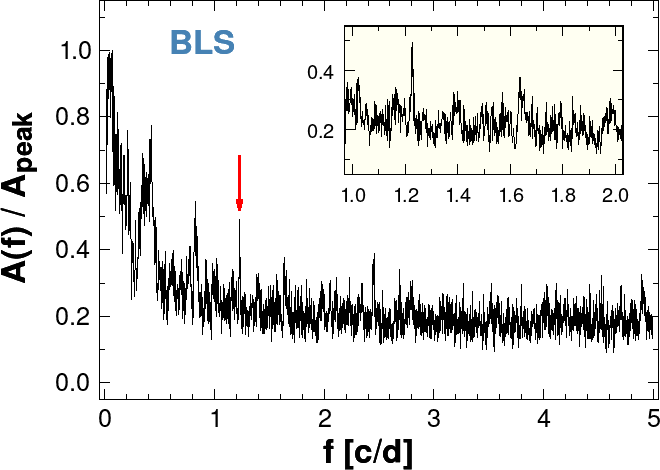
From the structure of the spectrum, it is clear that ppt transit depth is close to the low limit of a transit signal we can hope to detect in the available dataset. This limit is changing as a function of dataset and frequency, and is obviously higher for signals with periods longer than one day.
5 The eccentricity
With the occultation ephemeris derived in Sect. 3 and with the updated transit ephemeris by using the TESS data in Sect. 4, we can easily compute the two components of the eccentricity. For an easier reference, the components are as follows (Winn 2014)
| (20) | |||||
| (21) |
where and , respectively, are the observed (corrected for light-time effect) and calculated phases of the occultation centers (the latter is with the assumption of circular orbit). The argument of periastron is denoted by . As described in Sect. 3.3, the errors of the occultation signal in the Ks band were computed from a simple Monte Carlo simulation, based on the binned version of the merged data from the three data sources. The observational noise was considered to be multiplicative and non-stationary, according to the standard deviations around the bin means. For the realizations we calculated the eccentricity components from the fitted trapezoidal occultation parameters. As it is obvious from Eq. 20, the two components are not independent. Furthermore, is expected to be less noisy, as several authors noted previously (Winn 2014, e.g., ). Indeed, Fig. 10 clearly shows both the correlation and the considerably tighter behavior of . We also observe that the component is shifted to more positive values. This is because noise makes the ingress/egress parts shallower, leading to the preference of longer eclipse durations in the best-fit search.

From these simulations we obtained the errors also for the eccentricity components and, finally, for the eccentricity. For simple reference, we summarized these parameters in Table 5. The correlation between the two eccentricity components is also exhibited by the lower error on the eccentricity than that on the component.
It is instructive to compare our eccentricity values with those derived from the Spitzer data by Baskin et al. 2013. First we checked if there was any difference between using our transit ephemerides vs those employed by Baskin et al. 2013. We found that for the two epochs Baskin et al. 2013 published in their Table 1, our ephemerides predicted an average offset min greater than the one calculated from the ephemerides of Fukui et al. 2011 ( min vs min). Their offset time implies . Because the agreement is at the level between their value and ours, we can average them out and arrive at a value of , not implying anything different from zero eccentricity.1212 12 Baskin et al. 2013 did not publish values, so we cannot compare the eccentricities directly.
| Quantity | Value | Error |
|---|---|---|
| 0.00195 | ||
| 0.02197 | ||
| 0.01520 |
6 The emission spectrum
Here we examine how the more accurate occultation depth in the near infrared (Sect. 3.3) and our preliminary estimate on the same quantity in the visible from the TESS data (Sect. 4.2) can constrain the atmospheric properties of WASP-5 b. The secondary eclipse analysis was presented in Sect. 3, where we derived an occultation depth of ppt in the near infrared.
In the visible, corresponding to the wide-band filter of TESS1313 13 , m, see: http://svo2.cab.inta-csic.es/theory/fps/, we use the average of the eclipse depths obtained from four types of datasets: ppt. Although we could use also the value obtained from the estimation of the phase variation, we opted not to use this value for reasons discussed in Sect. 4.2.
Baskin et al. 2013 have measured the planet’s emission at m and m by the Spitzer infrared satellite. Although we do not make any model fitting in this paper – since we use the same models as given by Chen et al. 2014 –, we found it instructive to display all, currently available data on the same plot.
The atmospheric models presented by Chen et al. 2014 are based on the plane-parallel equilibrium models of Madhusudhan & Seager 2009; Madhusudhan & Seager 2010, employing free pressure–temperature profile and chemical composition. Figure 11 shows these theoretical spectra and the black body lines for fully efficient and zero circulations (Cowan & Agol 2011, i.e., lack of heat exchange between the day and night sides of the planet – see). The atmospheric models have monotonic pressure–temperature profile (i.e., no temperature inversion). The depth of the atmosphere was chosen to fit the brightness temperatures corresponding to the J, H, K data of Chen et al. 2014.
There are two essential conclusions we can draw from the positions of the new data points in respect to these models. First, the lower error bar on Ks increased the significance of the higher Ks flux and suggests strong emission in this waveband. This can be realized by additional emitters at a deeper level of the atmosphere (corresponding to temperatures higher than K).
Second, even though our estimate for the secondary eclipse depth is only tentative in the TESS band, it still yields a useful piece of information. This is because of the relatively small error on the data with respect to the spectral features in the optical. In particular, the current value of the emission in the visible corroborates what the Spitzer data may also indicate, i.e., no strong preference for any of models used.

From the optical occultation depth we can also estimate the geometric albedo. For an easier reference, here we repeat the necessary formulae presented by Cowan & Agol 2011 and, e.g., by Daylan et al. 2021. The observed occultation depth constitutes two parts: the thermal radiation by the planet and the reflected light of the host star
| (26) |
Assuming circular orbit, the reflected light is directly related to the geometric albedo
| (27) |
where is the planet radius, is the semi-major axis. The dayside thermal emission can be parameterized as follows
| (28) |
where is the stellar radius, and are the wavelength () dependent fluxes of the planet and the star, respectively. In the black body approximation, parameter is used to relate the substellar temperature to the dayside temperature
| (29) |
The single parameter comprises the Bond albedo and the atmospheric circulation parameter . For the origin of the coefficients in the expression of we refer to Burrows et al. 2008 and Cowan & Agol 2011. Obviously, separation of and is not possible by using the occultation alone. However, by measuring the phase curve, one may attempt to derive the night side emissivity that depends solely on (Singh et al. 2021). Because of the lack of very high quality data required by this method, we opted to parameterize the derived geometric albedo depending on the extreme limits of and omitting the negligible temperature decrease due to the expectedly small Bond albedo (Mallonn et al. 2019, e.g.,). Furthermore, as usual, we assumed pure black body radiations both for the star and for the planet in the waveband of interest.

The result is shown in Fig. 12. Although with fully efficient circulation () the geometric albedo can be as high as , based on the Ks occultation data (Kovács & Kovács 2019, e.g.,) and several other, more direct studies (Keating et al. 2019, i.e., those based on full phase curve analyses, such as) it is highly unlikely that WASP-5 b stands out from the other hot Jupiters, that mostly have low circulation efficiency. Therefore, it is quite reasonable to assume that the true value of is closer to the no circulation limit of .
7 Conclusions
In this work we dealt with the secondary eclipse (occultation) light curve of the hot Jupiter WASP-5 b. Our goal was twofold: i) derive accurate occultation light curve in the 2MASS Ks band, and, ii) use the latest TESS data to obtain the first estimate on the occultation depth in the optical. For goal i) we used already published Ks photometry by Chen et al. 2014 and Zhou et al. 2015 and combined these with the so far unpublished observations made by the FourStar infrared imager of the Baade 6.5 m telescope in 2011. Following the principle of “minimum data massage” we ended up with a high precision occultation light curve. The relative flux depression (planet vs star) is ppt, which places WASP-5 b among the top few extrasolar planets with Ks occultation light curve of relative precision this high.
We attempted to find the signature of secondary eclipse and phase variation in the visible by using the currently available TESS data from two visits. Based on the statistical tests presented in Appendix B we found convincing pieces of evidence that the underlying signals are unlikely to have total variation greater than ppt. As a result, we accepted the eclipse depth derived from the formal fit, i.e., ppt.
Using these values, our main conclusions on the atmospheric properties of WASP-5 b are as follows.
- •
Simple black body radiation fails to reach the observed Ks emission at the level of . A similar statement, with somewhat lower significance of %, is also true for the band-averaged values of the adopted atmospheric models. Detailed atmospheric modeling with strong emission features in the Ks band is required to fit the high observed emission.
- •
The value derived for the emission in the TESS waveband shows no preference for any of the adopted models with oxygen or carbon enhancements. The observed emission value is apart from both models.
- •
From the TESS eclipse depth we found that, depending on the circulation model, the geometric albedo is likely in the range of –. This places WASP-5b among the most reflective extrasolar planets but with a caveat of the preliminary nature of the detection of the secondary eclipse in the optical.
It is also worth mentioning that the ephemeris of the Ks occultation light curve further confirms the low (likely zero) eccentricity of the orbit, namely . Furthermore, the TESS data do not suggest the presence of any additional transiting planet larger than Earth radii with a period between and days.
The Ks waveband is within a relatively easy reach for most of the ground-based telescopes with near infrared capabilities. However, the time scale and the signal level make extrasolar occultation measurement still challenging, due to the combination of the above two properties with the local conditions, exhibited via the red noise component of the observed photometric time series. Perhaps the best way of handling red noise (if there are no other ways to filter it out), is to take multiple samplings. The careful combination of these samples will reduce both the white and red noise components. Due to the sparse sampling from the side of the available data points in the different wavebands, measurement accuracy is crucial for spectral retrieval. Although this spectral band is (will be) available in various space missions (Tinetti et al. 2018, JWST now and ARIEL by the end of the decade – see ), the expected high demand (in particular for JWST) makes ground-based observations still very important in supplying high quality data for more reliable extrasolar planet atmosphere modeling.
Acknowledgements.
Constructive comments by the referee are appreciated, in particular those that have led to a deeper investigation of the significance of the secondary eclipse in the TESS band. We thank Nikku Madhusudhan for the valuable comments regarding the atmospheric modeling of WASP-5b. This paper includes data collected with the TESS mission, obtained from the MAST data archive at the Space Telescope Science Institute (STScI). Funding for the TESS mission is provided by the NASA Explorer Program. STScI is operated by the Association of Universities for Research in Astronomy, Inc., under NASA contract NAS 5-26555. I.D. was supported by the Deutsche Forschungsgemeinschaft (DFG, German Research Foundation) – Project-ID 138713538 – SFB 881 (“The Milky Way System”, subproject A03). G.C. acknowledges the support by National Natural Science Foundation of China (Grant No. 42075122, 12122308). Support from the National Research, Development and Innovation Office (grants K 129249 and NN 129075) is acknowledged.References
- Alonso (2018) Alonso, R. 2018, Handbook of Exoplanets, ISBN 978-3-319-55332-0, id.40 (arXiv:1803.06204)
- Anderson et al. (2008) Anderson, D., Gillon, M., Hellier, C. et al. 2008, MNRAS, 387, L4
- Baluev et al. (2019) Baluev, R. V., Sokov, E. N., Jones, H. R. A. et al. 2019, MNRAS, 490, 1299
- Baskin et al. (2013) Baskin, N. J., Knutson H. A., Burrows, A. et al. 2013, ApJ, 773, 124
- Burrows et al. (2008) Burrows, A., Budaj, J., & Hubeny, I. 2008, ApJ, 678, 1436
- Charbonneau et al. (2005) Charbonneau, D., Allen, L. E., Megeath, S. T. et al., 2005, ApJ, 626, 523
- Chen et al. (2014) Chen, G., van Boekel, R., Madhusudhan, N. et al. 2014, A&A, 564, A6
- Cowan & Agol (2011) Cowan, N. B. & Agol, E. 2011, ApJ, 729, 54
- Croll (2015) Croll, B., Albert, L., Jayawardhana, R. et al. 2015, ApJ, 802, 28
- Daylan et al. (2021) Daylan, T., Günther, M. N., Mikal-Evans, T. et al. 2021, AJ, 161, 131
- Deming et al. (2005) Deming, D., Seager, S., Richardson, L. J., Harrington, J. 2005, Nature, 434, 740
- Fukui et al. (2011) Fukui A., Narita, N., Tristram, P. et al., 2011, PASJ, 63, 287
- Gillon et al. (2009) Gillon, M., Smalley, B., Hebb, L., et al. 2009, A&A, 496, 259
- Hoyer et al. (2012) Hoyer, S., Rojo, P. & Lopez-Morales, M. 2012, ApJ, 748, 22
- Irwin (2010) Irwin, M. J., 2010, UKIRT Newsletter 26, 14
- Ivshina & Winn (2022) Ivshina, Ekaterina, S. & Winn, Joshua, N. 2022, ApJS, (accepted, arXiv:2202.03401v2)
- Keating et al. (2019) Keating, D., Cowan, N. B., & Dang, L. 2019, NatAs, 3, 1092
- Kovacs et al. (2002) Kovacs, G., Zucker, S. & Mazeh, T. 2002, A&A, 391, 369
- Kovács & Kovács (2019) Kovács, G. & Kovács, T. 2019, A&A, 625, A80
- Kovacs (2020) Kovacs, G. 2020, A&A, 643, A169
- Madhusudhan & Seager (2009) Madhusudhan, N., & Seager, S. 2009, ApJ, 707, 24
- Madhusudhan & Seager (2010) Madhusudhan, N., & Seager, S. 2010, ApJ, 725, 261
- Mallonn et al. (2019) Mallonn, M., Köhler, J., Alexoudi, X. et al. 2019, A&A, 624, A62
- Martioli et al. (2019) Martioli, E.; Colón, K. D., Angerhausen, D. et al. 2018, MNRAS, 474, 4264
- Moyano et al. (2017) Moyano, M., Almeida, L. A., von Essen, C. et al. 2017, MNRAS, 471, 650
- Otegi et al. (2021) Otegi, J. F., Helled, R., & Bouchy, F. 2021, A&A, submitted (arXiv:2112.07413v1)
- Pál (2012) Pál, A. 2012, MNRAS, 421, 1825
- Poon et al. (2021) Poon, Sanson T. S., Nelson, Richard P., & Coleman, Gavin A. L. 2021, MNRAS, 505, 2500
- Ricker et al. (2015) Ricker, G. R., Winn, J. N., Vanderspek, R. et al. 2015, JATIS, 1, 014003
- Singh et al. (2021) Singh, V., Bonomo, A. S., Scandariato, G. et al. 2021, A&A, submitted (arXiv:2111.05716v1)
- Smith et al. (2012) Smith, J. C., Stumpe, M. C., Van Cleve, J. E. et al. 2012, PASP, 124, 1000
- Snellen & Covino (2007) Snellen, I. A. G.& Covino, E. 2007, MNRAS, 375, 307
- Stumpe et al. (2012) Stumpe, M. C., Smith, J. C., Van Cleve, J. E. et al. 2012, PASP, 124, 985
- Tinetti et al. (2018) Tinetti, G. Drossart, P., Eccleston, P. et al. 2018, ExA, 46, 135
- Werner et al. (2004) Werner, M. W., Roellig, T. L., Low, F. J., et al. 2004, ApJS, 154, 1
- Winn (2014) Winn, J. N. 2014, http://arxiv.org/abs/1001.2010v5
- Wong et al. (2020) Wong, I., Shporer, A., Daylan, T. et al. 2020, AJ, 160, 155
- Wong et al. (2021) Wong, I., Kitzmann, D., Shporer, A. et al. 2021, AJ, 162, 127
- Zhou et al. (2015) Zhou, G., Bayliss, Bayliss, D. D. R., Kedziora-Chudczer, L. 2015, MNRAS, 454, 3002
Appendix A Trapezoidal fits to the nightly Ks data
Notes: The ingress and egress phases (, ) can be converted into Barycentric Julian Date (TDB standard) by the following formulae: [BJD], where is the epoch number of the event of interest and is the moment of the transit center, d – see Sect. 4.1 for more details. The epochs are without correction for orbital light time effect.
| Set | |||||||
|---|---|---|---|---|---|---|---|
| (phase) | (phase) | (phase) | (phase) | () | () | ||
| 1 | |||||||
| 2 | |||||||
| 3 | |||||||
| 123 |
In this Appendix we give further details of the method of the error estimation of the trapezoidal fit. This section serves also the closer assessment of the improvement resulted from merging the three datasets available in Ks color.
The individual nightly data by Chen et al. 2014, this paper and Zhou et al. 2015 are fitted by the trapezoidal model of Sect. 3.1. The procedure followed for the individual datasets is the same as described in Sect. 3.3. The starting time series are the light curves that have already been filtered out from systematics and major outliers (see Fig. 4). To include the effect of changing noise level (both random and left-in systematics) throughout the night, the light curves were binned and the average bin values were used as the starting light curve of the simple Monte Carlo simulations. These simulations were performed with noise realizations superposed on this “noiseless” light curve. The standard deviation of the superposed Gaussian noise changed according to the standard deviation of the observed data in each bin.
We used overlapping bins, i.e., the total time span of a given dataset was divided into equal time segments and the averages and standard deviations of the data points belonging to each of these segments were calculated. Then, the overlapping sequence started at half of the first bin and continued until the half of the last bin. The bin width of the second sequence was somewhat shorter, because we generated the same number of bins (i.e., ) as for the first sequence. Finally, all the bin averages and standard deviations were assigned to the bins of equal length filling in the full time span. This method of bin generation was used for all three datasets, independently of their lengths. While generating the mock light curves for noise estimation, we mapped back the bin statistics to the original timebase by choosing the bin values at the given time (or phase) value of the unbinned time series.
The simulated light curves served as inputs for our robust trapezoidal fitting routine. The resulting parameters were used to compute their standard deviations ( errors). The trapezoidal parameters themselves were obtained from a direct fit to the original (unbinned) data. In searching for the best fit, we used simple parameter scanning in the following ranges (in the units of the orbital phase): , , , corresponding to phase change for with respect to a finally accepted best-fit value. The scanning ranges in and correspond to % relative variations (again, with respect to the same final best-fit values). Except for , we had very rare hits at the limiting values. The more frequent hits for can be tolerated on the ground of the limits imposed by the known system parameters.
The result is shown in Table 6. To make the comparison easy, we copied the result of the analysis of the merged data from Table 2 in the fourth row. In the last but one column we show the standard deviation of the fit to the original data. The errors of the standard deviation of come from the Monte Carlo simulations and indicate the data point number dependence of the statistical stability of the realizations.
We see that the merged data yield a considerable improvement with respect to all datasets. With an overall error decrease of %, a relative modest improvement can be observed for set-2. For the other sets we find improvement in the range of –%. It is also observable that while our transit depth error is in agreement with the one derived by Zhou et al. 2015 there is nearly a factor of two difference between our error of ppt, vs that of Chen et al. 2014. It is quite likely, that the latter estimate ( ppt) is closer to the real error, since their estimate follows the full sequence of light curve evaluation (which is certainly very sensitive to the method of systematics treatment), whereas our estimate relies on their “final product”. However, at the end, from the point of view of the merged data analysis, the weight of this dataset is relatively small, due to the small number of data points.
Appendix B Testing occultation and phase variation limits from TESS
We performed eclipse and phase variation analyses on the full set of TESS light curves – including sectors and . With the option of polynomial filtering (see Sect. 4), we have four types of datasets to be analyzed (SAP and PDC, with or without polynomial filtering). The time series models were incomplete – i.e., they contained either an occulation or a phase variation signal. This is a reasonable approximation in the high noise regime, when focusing on the detection limits of signals with very different time dependences.
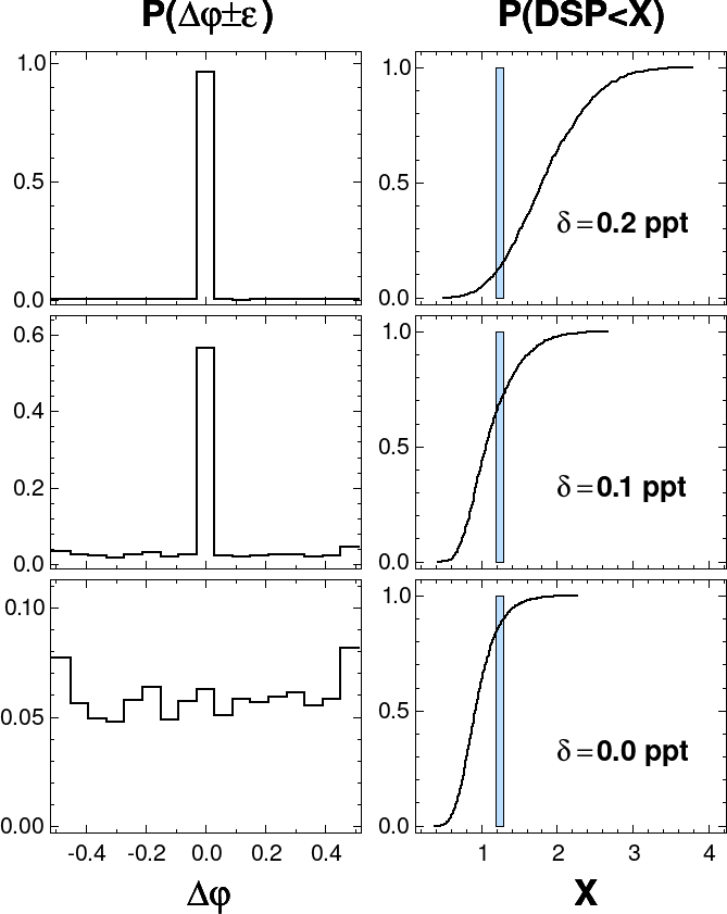
For the eclipse dip search, the folded light curve was approximated by a bin model, with equal widths for all bins, equal to that of the transit. The distribution of the bins was fixed, as given by the predicted phase of the secondary eclipse. The bin average yielding the largest flux depression and the center phase of that bin yields, respectively, the estimated eclipse depth and eclipse phase . To characterize the quality of this representation of the eclipse, we used the dip significance parameter (DSP) as defined in Kovacs 2020
| (36) |
where is the error of the eclipse depth , is the standard deviation of the bin averages for the bins outside the eclipse, is the standard deviation of the successive differences between the same bin averages. The last two terms are devoted to account for both regular, smooth variations () and irregularities originating from pure noise at the phase scale of the bins (). The DSP value associated with the deepest bin average (i.e., the largest ) was used to characterize the quality of the eclipse solution for a given dataset. It is noted that for a complete signal, DSP is limited by the second term in the denominator, due to the near equality of the eclipse depth and the total amplitude of the phase variation. Figure 13 shows the relation between the light curve quality and the above parametrization.

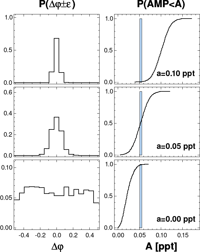
The phase variation search was performed by a simple two-parameter ( and ) least squares fit of a cosine function . With a good approximation, the amplitude of the cosine is half of the occultation depth (Daylan et al. 2021, e.g.,). The quality of the cosine model is characterized by the signal-to-noise ratio , which – as expected – for low-SNR signals, like the ones studied here, is tightly correlated with .
The results of the above separate fits for the four types of datasets are displayed in Table 7. Although there are differences among the datasets, the properties of the signals are largely stable. The box fit yields remarkable coincidence with the expected occultation center. On the other hand, the maximum of the cosine is systematically shifted, and precedes the occultation center in phase by . The amplitude of the phase variation and the eclipse depth are consistent within the error limit: ppt vs ppt.
| DATA | BIN fit | COSINE fit | ||||||
|---|---|---|---|---|---|---|---|---|
| Type | Pol | [ppt] | [ppt] | DSP | [ppt] | SNR | ||
| SAP | 0 | 2.84 | 0.00 | 1.09 | 1.90 | |||
| SAP | 1 | 2.49 | 0.00 | 1.11 | 3.07 | |||
| PDC | 0 | 2.35 | 0.00 | 1.24 | 3.50 | |||
| PDC | 1 | 2.32 | 0.00 | 1.24 | 2.94 | |||
Notes: Pol: for with or without polynomial filtering; : standard deviation of the input time series; for the bin model and for the cosine model; : eclipse depth; DSP: dip significance parameter; A: amplitude of the cosine fitted; SNR: signal-to-noise ratio for the cosine fit. See text for additional information on the symbols.
It is important to address the statistical significance of these, obviously near noise-level detections. To do so, we performed simple Monte Carlo simulations by generating the following type of signals
| (43) |
where is an uncorrelated Gaussian noise with standard deviations shown in Table 7. Function is either a simple box or a cosine function, representing the secondary eclipse or the phase variation. The box model is zero out of the eclipse and within the eclipse, with the box centered at the phase of the assumed eclipse, ( phase after the transit). Probability density functions (PDFs) and cumulative distribution functions (CDFs) were computed for the phase differences (i.e., ), DSP and A values.
The primary goal of this investigation is to pose an upper limit on the underlying signal by using the near noise-level values derived above. Therefore, we computed two basic quantities. In the presence of injected signals of varying amplitudes and box depths we computed: a) the occurrence rates of box depths and cosine amplitudes less than the observed values; b) the occurrence rates of the dip center and cosine maximum phases within the proximity of the predicted secondary eclipse.
As an example, for three different injected box signals, Fig. 14 shows the PDF of the phase differences and the CDFs of the DSP values. The phases seem to converge quite quickly (i.e., even for boxes as shallow as ppt, more than half of the cases hit the near proximity of the expected phase). It is interesting to note that there is surplus of occurrences at the edges in the phase distribution. It is especially visible in the pure noise () simulations. The reason of this excess is the smaller number of data points in the bins at the end-phases of the folded time series (the bin occupancy depends on the positioning of the occultation and the width of the eclipse). This leads to more fluctuating values at the edges, and therefore, higher chance of being selected as the “best-fit” for the box model.
The DSP values are less sensitive to a small underlying signal. They are still near the pure noise values and they become more distinctive from these only if the box depths become deeper than ppt.
A similar test performed on the same type of dataset with injected cosine signals indicate the opposite effect (see Fig. 15). The phase settles at a far lower pace but the amplitude of the signal becomes more quickly detectable. For example, if the underlying cosine signal had an amplitude of ppt (corresponding to an eclipse depth of ppt), then the probability that we can detect a component as low as observed is less than .
We can assess the likelihood of the various underlying signals in the currently available TESS data by using the data settings (i.e., data point distribution, N and ) for the two extreme data types shown in Table 7. These settings correspond to the PDC and SAP fluxes, respectively, with and without polynomial detrending. We utilize the detection power of the phase of the bin search and the amplitude sensitivity of the Fourier fit. The upper panel of Fig. 16 shows the occurrence rate of the observed total amplitude as a function of the underlying (injected) signal amplitude. The lower panel exhibits the likelihood that the best-fitting bin phase is not being in the close proximity of the predicted phase.

These plots suggest that the underlying phase variation should have a total amplitude less than ppt with a probability of more than %, because otherwise it would have a probability less than % to get a cosine amplitude as small as given in Table 7. Although at a somewhat lower level of significance, this result is corroborated by the frequency of the correct phase hits in the box test. Depending somewhat on the data type, the probability of not hitting the correct phase for an underlying boxy eclipse signal of depth ppt is between % and %. We note that the average of the eclipse depths derived from the observed data and the associated formal error yield an upper limit of ppt, close to the high-significance limit obtained above. This, together with the stability of the observed eclipse phases, lend further support to the tentative detection of the secondary eclipse for WASP-5b from the TESS data.