String theory[1, 2] offers a consistent and finite quantum theory of gravity which can include the matter states and gauge symmetries that form the basis for the Standard Model (SM). The price to pay is that string theory must be formulated in 10 (or 11 for $M$-theory) spacetime dimensions. To gain our observable four spacetime dimensions, the additional space dimensions are assumed compactified into a tiny compact manifold such as a Calabi-Yau space (which preserves some spacetime supersymmetry (SUSY) under compactification). The resultant 4-d theory then consists minimally of the supersymmetric SM (MSSM) plus at least an assortment of gravitationally coupled scalar fields (the moduli) with no classical potential. The moduli fields, which parametrize the size and shape of the compact space, must be stabilized and then their vacuum expectation values (vevs) determine many features of the low energy 4-d effective theory such as coupling constants and soft SUSY breaking terms. Typical string compactifications then contain, in the 4-d limit, on order of tens-to-hundreds of moduli fields in addition to visible and hidden sector fields.

In II-B string theory, the moduli can be classified as complex structure ($U_{\alpha}$) and Kähler ($T_{\beta}$) along with the axio-dilaton ($S$). Under flux compactifications[3], the $S$ and $U_{\alpha}$ moduli are stabilized by flux and should gain ultra-high KK-scale masses. Under KKLT stabilization[4], the $T_{\beta}$ are stabilized non-perturbatively while in LVS stabilization[5], the $T_{\beta}$ are stabilized by a balancing of perturbative and non-perturbative effects. Thus, the Kähler moduli may have much lighter masses which may be as low as the soft SUSY breaking scale $m_{soft}\sim 1$ TeV. The lightest of the moduli, $\phi$ (with mass labeled here as $m_{\phi}$) may be cosmologically dangerous in that

1. 1.

   they may live long enough to decay after the onset of BBN thus destroying the successful BBN predictions of light element abundances[6, 7, 8],

2. 2.

   they may overproduce neutralino dark matter (the moduli-induced LSP problem)[9],

3. 3.

   they may overproduce gravitinos if $m_{\phi}>2m_{3/2}$ (the moduli-induced gravitino problem)[10, 11, 12, 13, 14] where then the gravitinos could decay after onset of BBN or overproduce dark matter and

4. 4.

   they may decay into relativistic particles such as the axion-like particles (ALPs)[15, 16] which are endemic to 4-d string models[17], thus potentially violating limits on dark radiation as parametrized by the parameter $N_{eff}$, the effective number of light neutrinos which inhabit the cosmic soup.

Under KKLT stabilization, the shift symmetry $T\rightarrow T+i\alpha$ is destroyed and the corresponding ALPs, which comprise the phase fields of the $T_{\beta}$, are expected to obtain masses comparable to the corresponding real components: $m_{\text{A}LP}\gtrsim m_{soft}$. However, for LVS stabilization, the shift symmetry can survive, and the corresponding ALPs end up with small but non-zero masses and thus may comprise a portion of the measured dark radiation.

Indeed, years ago the measured value of $N_{eff}$ seemed somewhat displaced from the SM value, motivating great excitement that string remnants may have left a detectable imprint on the cosmic microwave background radiation (CMB). In recent years, increasingly precise CMB measurements have brought $N_{eff}$ more into accord with SM expectations, so that $\Delta N_{eff}$ provides now increasingly tight constraints on new physics models which include dark radiation.

The 2018 Planck analysis of cosmological parameters[18] in relation to CMB measurements is able to fit the amount of dark radiation at 95% CL as

based upon joint fits to Planck CMB polarization, lensing and baryon acoustic oscillations (BAO). From these fits, and using the Standard Model (SM) value $N_{eff}(SM)=3.046$[19], we will require that at 95% CL

In this paper, we continue our earlier investigation[20] of the cosmological moduli problem (CMP) wherein we computed the various modulus decay rates into the MSSM particles including all phase space and mixing effects which are routinely ignored in the literature. Once these are known, then one may compute the modulus decay temperature $T_{D}\simeq\sqrt{\Gamma_{\phi}m_{P}}/(\pi g_{*}/90)^{1/4}$ and use these to implement BBN constraints ($T_{D}>T_{BBN}\sim 3-5$ MeV). One may also compute the modulus oscillation temperature $T_{osc}$, the modulus-radiation equality temperature $T_{e}$, and the temperature $T_{3/2}$ of radiation at the time of gravitino decay. Comparing to the inflaton reheat temperature $T_{R}$ and neutralino freeze-out temperature $T_{fo}$, then one may compute the entropy dilution factor $r=S_{f}/S_{0}=T_{e}/T_{D}$ and the ultimate non-thermal neutralino abundance and constraints on relic gravitinos. Assuming a well-motivated natural SUSY spectrum of MSSM particles, it was found that very large modulus masses $m_{\phi}\gtrsim 5000$ TeV were needed (assuming an initial modulus field strength $\phi_{0}\sim m_{P}$) to avoid the moduli-induced LSP problem. Also, typically $m_{\phi}<2m_{3/2}$ was needed to avoid the moduli-induced gravitino problem. For the well-motivated gravity-mediated SUSY breaking model, wherein the soft SUSY breaking scale $m_{soft}\sim m_{3/2}$, then the high mass modulus solution to the CMP would bring physics into conflict with naturalness of SUSY models which requires sparticles (save light higgsinos) typically in the several TeV range[20]¹¹ 1 For natural SUSY models, we require models to have low electroweak finetuning with $\Delta_{EW}\lesssim 30$[21, 22].. An alternative solution which allows much lighter values of $m_{\phi}\sim 30$ TeV is to find an anthropic selection on modulus field strength $\phi_{0}\sim 10^{-7}m_{P}$ which allows for a more comparable dark-matter-to-baryonic-matter ratio $\sim 1-10$[23]. Alternatively, $m_{\phi}\sim m_{weak}$ with $\phi_{0}\sim m_{P}$ leads to a dark matter dominated universe wherein baryons might only occur as diffuse hardly gravitating clouds and minimal structure for baryonic matter[24, 25, 26].

In the present work, we extend our previous analyses to include the effects of modulus decay into ALPs, which may occur for LVS moduli stabilization, but may occur more generally in other (possibly unthought of) 4-d string models. This addresses a fourth facet of the CMP: the moduli-induced ALP problem[15, 16, 27]. But first, we review several related works that precede our contribution, and explain the new aspects of our own work. Then in Sec. 2, we explain our calculation of modulus field coupling to ALPs and decay rate into dark radiation. In Sec. 3, we present details of our calculation of $\Delta N_{eff}$ in the sudden decay approximation and in Sec. 5 we present numerical results which mainly restrict the values of $m_{\phi}$ and modulus-ALP coupling $\lambda_{\text{A}LP}$. We find that in spite of the tightening error bars from the experimental determination of $\Delta N_{eff}$, the moduli-induced ALP problem is perhaps not overly constraining, even for values of $\lambda_{\text{A}LP}\sim 1$, unless $m_{\phi}$ is very large $m_{\phi}\gtrsim 10^{4}$ TeV wherein the modulus field begins to oscillate before the end of inflation (where $T_{osc}\gtrsim T_{R}$, assuming a reheat temperature of $T_{R}\sim 10^{12}$ GeV). On the other hand, the anthropic solution to the moduli-induced LSP problem does not help much with the modulus-induced ALP problem since decreasing the field strength $\phi_{0}$ hardly affects the $\phi\rightarrow ALPs$ branching fraction. A brief summary and conclusions are given in Sec. 6.

We begin discussion of modulus decays into ALPs by briefly reviewing how the interaction arises within the Kähler potential. After describing how this arises in concrete moduli stabilization scenarios, we then illustrate our “stabilization-agnostic” approach.

The Kähler potential for the lightest geometrical moduli typically takes the approximate form

where $n_{i}$ is determined by the form of the compactification manifold volume, $\mathcal{V}$. In minimal LVS models, the volume is assumed to be of the form $\mathcal{V}\propto\tau_{b}^{3/2}$ (where $\tau_{b}$ is the “big” volume modulus) so that $n\simeq 3$, which gives the required “no-scale structure”[47, 48]. The volume may however take more complicated forms depending on the compactification details. In e.g. fibred LVS models such as those considered in [37], the volume of the compactification manifold instead goes as $\mathcal{V}\propto\sqrt{\tau_{1}}\tau_{2}$ - corresponding to a Kähler potential $K\supset-\log(T_{1}+\overline{T}_{1})-2\log(T_{2}+\overline{T}_{2})$ for the light geometrical moduli.

The Kähler metric associated to Eq. 3 is diagonal with entries $K_{ii}\simeq\frac{n_{i}}{4\tau_{i}^{2}}$, so that the (non-canonical) kinetic term in the Lagrangian becomes

where the $T_{i}=\tau_{i}+ic_{i}$. Through the field redefinitions

the canonical kinetic terms are recovered and after expanding the exponential, we obtain the interaction terms:

where we have now explicitly restored $m_{P}$. The form of this interaction term loosely matches the expectation for a $\phi_{i}a_{i}a_{i}$ interaction where the $a_{i}$ terms possess a shift symmetry. The coupling here is then set explicitly by the field space geometry. However, for models with more than one light modulus, the $\phi_{i}$ fields may still need to get rotated into the mass eigenbasis. While the specific form of the mass matrix is determined by the moduli stabilization details and hence is model dependent, the generic feature is that each modulus mass eigenstate may then decay to multiple ALP types, $a_{i}$, with couplings determined by $n_{i}$ and the form of the mass matrix.

In this work, we take the general form of Eq. 6 but make some minor adjustments. We begin by first writing down the interaction term as

Here, we assume that the lightest modulus $\phi$ is written in the mass eigenbasis. Since that may introduce couplings to multiple ALPs $a_{i}$ (which we expect to be nearly massless if the shift symmetry is preserved and kinematically inaccessible if the symmetry is broken), we choose to parameterize this by a single ALP field $a$ with an effective coupling $\lambda_{\rm ALP}$. The $\lambda_{\rm ALP}$ coupling then parameterizes the “total” coupling between the lightest modulus and the (possibly many) ALPs it may decay into, without relying on a specific stabilization model. In the familiar case of minimal LVS, we have $\lambda_{\rm ALP}=\sqrt{2/3}\simeq 0.816$. Larger values of $\lambda_{\rm ALP}\gtrsim 0.816$ can then parameterize decays to multiple ALPs, whereas $\lambda_{\rm ALP}\lesssim 0.816$ may correspond to some (possibly yet undiscovered) stabilization scheme in which the shift symmetry is broken for some ALPs coupled to $\phi$, making those decays kinematically forbidden and hence lowering the effective coupling.

The matrix element squared for this decay, taking for now a small but non-zero ALP mass, is

The decay width can then be easily computed:

Taking the massless limit for the ALPs $a$, the decay width simplifies to:

In the case of e.g. minimal LVS with $\lambda_{\rm ALP}=\sqrt{2/3}$, we recover the results in [15, 16].

Our task now is to quantify the amount of dark radiation produced in the early universe via modulus decay. As these light, relativistic degrees of freedom should contribute to the total radiation energy density, $\rho_{R}^{tot}$, it is useful to parameterize the radiation density as

Here, $T_{\nu}$ is the neutrino temperature and $T$ is the temperature of the thermal bath, related by $T_{\nu}=(\frac{4}{11})^{1/3}T$ [49]. In the SM, $N_{eff}^{SM}=3.046$ [19]. Any additional light degrees of freedom then correspond to an increase in $N_{eff}$ from its SM value, $\Delta N_{eff}=N_{eff}-N_{eff}^{SM}$. We can then estimate $\Delta N_{eff}$ from modulus decay into ALPs by

where $\rho_{\nu}$ is the energy density of a single neutrino species so that $\rho_{\nu}=\frac{7}{8}\frac{\pi^{2}}{15}T_{\nu}^{4}$.

Since the ALPs dilute as radiation, we can relate their energy density between $T_{D}$ and $T$ (with $T<T_{D}$) as

where we assume conservation of entropy density, $s=\frac{2\pi^{2}}{45}g_{*S}T^{3}$, between $T_{D}$ and $T$.

What remains is to calculate $\rho_{\text{ALP}}(T_{D})$. Here, to gain the overall big picture, we adopt the sudden decay approximation. Non-sudden effects will be included in forthcoming coupled Boltzmann calculations. Using conservation of energy density, we can then express the energy density of the ALPs in terms of the modulus:

where $r\equiv S_{f}/S_{i}=T_{e}/T_{D}$ is the entropy dilution factor[50, 51].

As the modulus behaves as non-relativistic matter, to estimate $\rho_{\phi}(T_{D})$ we first need the number density at $T_{D}$, which is given by

Putting all of this together, we arrive at the expression for $\Delta N_{eff}$

where for convenience we show $g_{*S}$ as a function of $T=m_{\phi}$ in Fig. 1.

Furthermore, we note that the temperature of radiation/modulus energy density equality, determined by requiring $\rho_{R}=\rho_{\phi}$, is found to be[51]

and where the oscillation temperature is found to be

where $m_{P}\equiv M_{Pl}/\sqrt{8\pi}$ is the reduced Planck mass.

In Eq. 15, we found that the amount of dark radiation depends directly on the modulus field branching fraction to ALPs. From Eq. 19, we expect the branching fraction ${\cal B}(\phi\rightarrow ALPs)$ to be of order $\sim 0.01-0.1$, although this approximate expression assumes that the modulus decay to SM modes includes only massless gauge bosons. The actual result can be very model-dependent in that various MSSM decay modes may be suppressed or not, and these details can seriously affect the ultimate modulus branching fraction into DR.

Recently, in Ref. [20], all MSSM decay modes of light moduli fields were computed assuming Moroi-Randall operators[52]. The decay widths were evaluated including all mixing and phase space effects. Even so, some of these decay modes are still model dependent. In particular, modulus decay to gauginos may or may not be helicity suppressed. The helicity suppression is displayed in the decay widths by whether or not the width numerator contains a factor $m_{\phi}^{3}$ (unsuppressed, case A) or $m_{\phi}m_{\lambda}^{2}$ (helicity-suppressed, case B). The suppression factor depends on details of the gauge kinetic function[11, 14]. Likewise, modulus decay to gravitinos may not be (case 1) or may be (case 2) helicity-suppressed depending on details of the Kähler function $K$[11, 14].

In addition, the moduli branching fractions depend on the specific details of the assumed SUSY particle mass spectrum. In Ref. [20], a natural SUSY benchmark (BM) spectrum was adopted with low finetuning measure $\Delta_{EW}\sim 20$. The BM point came from the NUHM3 model with parameters $m_{0}(1,2)=10$ TeV, $m_{0}(3)=5$ TeV, $m_{1/2}=1.2$ TeV, $A_{0}=-8$ TeV and $\tan\beta=10$. It also had $\mu=200$ GeV and $m_{A}=2$ TeV. Using the Isasugra spectrum calculator[53], it is found to have $m_{h}=125.3$ GeV and $m_{\tilde{g}}=2.9$ TeV– in accord with LHC Higgs mass measurement and sparticle mass limits. Such a point is expected to emerge with a high probability (relative to finetuned models) from string landscape selection[54, 55].

In Fig. 2, we plot the various modulus to MSSM particle partial widths as in Ref. [20] for the BM point in scenario B1, except here we also include the partial width for decay to ALPs (brown curve). As $m_{\phi}$ increases, most of the partial widths increase as $\Gamma_{\phi}\sim m_{\phi}^{3}$ as commonly assumed in the literature. However, here we see the partial widths to gauginos (and also SM fermion pairs) increases only as $\Gamma_{\phi}\sim m_{\phi}^{1}$ due to the assumed helicity suppression. Furthermore, the partial widths into MSSM sfermion pairs suffers additional suppression and so $\Gamma_{\phi}(\phi\rightarrow sfermions)\sim m_{\tilde{f}}^{4}/(m_{\phi}m_{P}^{2})$ and thus these partial widths decrease with increasing $m_{\phi}$. The important result is that there are very many MSSM decay modes, making the ultimate modulus BF into DR very model dependent. In much of the literature, it is assumed instead just that $\Gamma_{\phi}(\phi\rightarrow ALPs)\sim\Gamma_{\phi}(\phi\rightarrow MSSM)$.

In Fig. 3, we show the resultant branching fraction ${\cal B}(\phi\rightarrow\ ALPs)$ for the same BM case and scenario B1 (blue curve) as in Fig. 2. From the plot, we see that initially at low $m_{\phi}$ the BF oscillates somewhat due to turn on of various MSSM decay modes. Ultimately, the ${\cal B}(\phi\rightarrow ALPs)$ settles down to $\sim 1.4\times 10^{-2}$. The rather low $BF$ result, compared to other estimates in the literature, is due to our assumption in taking all couplings $\sim 1$, so that the gauge boson modes (and not the Higgs modes) are dominant - whereas in the explicit sequestered models usually studied for DR, the gauge bosons typically possess a loop suppression factor. The inclusion of the very many possible MSSM modes entering the modulus decay width then suppresses this branching ratio further to the percent level.

Also in Fig. 3, we show the modulus branching fraction ${\cal B}(\phi\rightarrow ALPs)$ versus $m_{\phi}$ for the same SUSY BM point but in decay scenario B2 (orange curve). This time we assume in addition that the $\phi$ decay modes to Higgs and matter superfields are turned off, as might be expected if these fields carry Peccei-Quinn (PQ) charges and are involved in a solution to the strong CP problem with a Kim-Nilles[56] solution to the SUSY $\mu$ problem[57]. Although the B2 scenario is quite different from scenario B1, the branching fractions are rather similar since the decays into MSSM particles are dominated by decays to gauge bosons.

Now that the modulus branching fraction to ALPs is estimated, we can proceed to using Eq. 15 to evaluate $\Delta N_{eff}$ numerically, including all MSSM decay modes. Our main result is shown in Fig. 4 where we plot $\Delta N_{eff}$ vs. $m_{\phi}$ for the case of our SUSY BM point and in scenario B2. The horizontal dashed red line denotes the Planck 2018 95% CL bound on $\Delta N_{eff}$, i.e. one is constrained to live below the red dashed line. We also show the projected limit of the Stage 4 CMB experiment[58] where $\Delta N_{eff}$ as low as 0.06 may be detected (dot-dashed line). We also show the value of $\Delta N_{eff}$ computed from Eq. 15 assuming three values of $\lambda_{\text{A}LP}=1,\ 2$ and the minimal LVS value of $0.816$. From the plot, we see that much of the green curve for $\lambda_{\rm ALP}=2$ would be excluded, while the remaining curves are excluded at very low $m_{\phi}\sim 1-2$ TeV. As $m_{\phi}$ increases, one might naively expect $\Delta N_{eff}$ to increase as $m_{\phi}^{2}$ according to Eq. 15. But for most of the range, the denominator $T_{e}T_{osc}^{3}\sim m_{\phi}^{2}$ as well, so that the $m_{\phi}$ dependence roughly cancels out. Instead, the bulk of $m_{\phi}$ dependence comes from the $g_{*}$ degrees of freedom parameters: namely, as $m_{\phi}$ increases, then $T_{D}$ and $T_{osc}$ also change and consequently the various values of $g_{*}$ change. For convenience, we plot in Fig. 1 the value of $g_{*S}(T)$ vs. $T=m_{\phi}$. Here, we see that as various thresholds are passed, then the effective number of MSSM degrees of freedom can increase significantly leading to the various slope discontinuities in $\Delta N_{eff}$ of Fig. 4.

Back to Fig. 4, we see that as $m_{\phi}$ increases past $\sim 2$ TeV, then $\Delta N_{eff}$ drops well below the Planck 95% CL bound for $\lambda_{\text{ALP}}\lesssim 1$ and stays in the allowed region all the way until $m_{\phi}\gtrsim 20,000-30,000$ TeV whence $\Delta N_{eff}$ begins a sharp increase into forbidden territory. The sharp increase is due to the fact that $m_{\phi}$ is so large that $\phi$ starts oscillating earlier than our assumed value of reheat temperature $T_{R}\sim 10^{12}$ GeV, i.e. that the field $\phi$ begins oscillating before the reheating period of inflation has finished. In this case, the dependence of $T_{e}$ and $T_{osc}$ changes as in Eq’s 16 and 17 and the value of $\Delta N_{eff}$ consequently increases with increasing $m_{\phi}$.

Thus, the bulk of the region for $m_{\phi}\sim 2-30,000$ TeV is allowed by present CMB data if $\lambda_{\text{ALP}}\lesssim 1$. Furthermore, the $\Delta N_{eff}$ distribution reaches a minimal value in $\Delta N_{eff}\sim 0.04-0.28$ for $m_{\phi}\sim 700-6000$ TeV. This is the same value of $m_{\phi}$ for which the dark matter abundance $\Omega_{\chi}h^{2}$ drops into the allowed region $\lesssim 0.1$ in Ref. [20]. Thus, for these very heavy values of $m_{\phi}$, both the modulus induced BBN, DM and DR problems are all solved. A remaining outlier problem would be the moduli-induced gravitino problem for $m_{\phi}\gtrsim 2m_{3/2}$. Assuming $m_{3/2}\sim m_{soft}$ as in gravity mediation, then one is faced with antagonism between SUSY naturalness requiring TeV-scale soft terms and a solution to the various CMP problems which may favor much heavier moduli masses[20].

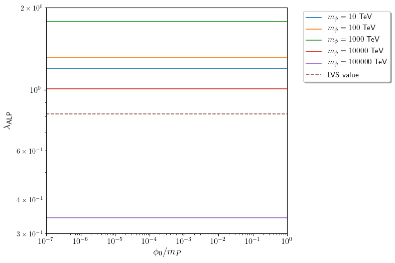
One way to reconcile the four CMPs with naturalness is to assume the lightest modulus $\phi$ is stabilized by SUSY breaking so that $m_{\phi}\sim m_{soft}\sim m_{3/2}$ so the gravitino decay mode is closed but with $m_{\phi}\sim 1-10$ TeV. The anthropic solution[23] to the CMPs then selects low $\phi_{0}$ values $\sim 10^{-7}m_{P}$ in order to gain a comparable DM-to-baryons abundance. Notice that the tiny $\phi_{0}$ value does not suppress the ${\cal B}(\phi\rightarrow ALPs)$ since $\phi_{0}$ tends to cancel in Eq. 15. To show this more clearly, we plot in Fig. 5 the upper bound on $\lambda_{\text{A}LP}$ versus $\phi_{0}/m_{P}$ which is required to stay below the Planck CMB limit on $\Delta N_{eff}$ for various values of $m_{\phi}$. For most $m_{\phi}$ values, the upper bound on $\lambda_{\text{A}LP}$ exceeds the naive LVS limit although for $m_{\phi}\sim 10^{5}$ TeV the upper limit drops to $\lambda_{\text{A}LP}\lesssim 0.31$. Thus, for much of the range of $m_{\phi}$, assuming the bulk of $\phi\rightarrow MSSM$ decay modes are open, the DR aspect of the CMP does not seem too severe, at least at present. On the other hand, at least for the LVS stabilization scheme, one might expect a good chance for a future deviation in the measured value of $\Delta N_{eff}$ compared to the SM value.

In this paper, we have continued our exploration of the various aspects of the CMP, this time addressing the issue of dark radiation coming from the lightest modulus $\phi$ decay to its associated ALPs. In this work, we have neglected a so-called PQ sector QCD axion which may behave differently from a light stringy ALP in that its interactions would be suppressed by the PQ scale $f_{a}$ instead of $m_{P}$ and its mass and couplings would be related as in the PQ solution to the strong CP problem[59]. For the SUSY PQ model, then one also expects the presence of saxions and axinos which can all affect the various particle abundances. In future work, we intend to include light moduli fields into previous eight-coupled Boltzmann solutions to the dark matter abundance from mixed axion-neutralino dark matter[60, 31, 61].

Our present work extends previous work[23, 20] by including modulus field decay to its associated ALP particle assuming the ALP mass is quite light as should occur in the LVS moduli stabilization scheme wherein moduli are stabilized by a combination of perturbative and nonperturbative effects. In other models such as KKLT with purely non-perturbative Kähler moduli stabilization, then the ALPs tend to get masses comparable to the moduli, and there is no ALP dark radiation problem. Our present analysis has been more phenomenological, not restricting ourselves to a particular stabilization scheme since for more realistic CY manifolds, one expects far more Kähler moduli than the few that are assumed in simple toy moduli stabilization schemes. In the more general case, where the full panoply of MSSM decay modes of the lightest modulus may be allowed and the gauge boson decay modes may be allowed at tree level, then the modulus branching fraction to dark radiation is typically $\sim 0.01$, lower than is usually assumed. In such cases, where $m_{\phi}>2m_{\rm ALP}$, then typically the $\Delta N_{eff}$ is below present limits. Future experiments such as Stage 4 CMB (CMB-S4)[58] are expected to probe much smaller $\Delta N_{eff}\sim 0.06$. If so, then a discrepancy could still appear for light enough ALP particles coming from string compactifications.

Acknowledgements:

This material is based upon work supported by the U.S. Department of Energy, Office of Science, Office of High Energy Physics under Award Number DE-SC-0009956 and U.S. Department of Energy (DoE) Grant DE-SC-0017647.

References

- [1] M. B. Green, J. H. Schwarz, E. Witten, SUPERSTRING THEORY. VOL. 1: INTRODUCTION, Cambridge Monographs on Mathematical Physics, 1988.
- [2] M. B. Green, J. H. Schwarz, E. Witten, SUPERSTRING THEORY. VOL. 2: LOOP AMPLITUDES, ANOMALIES AND PHENOMENOLOGY, 1988.
- [3] M. R. Douglas, S. Kachru, Flux compactification, Rev. Mod. Phys. 79 (2007) 733–796. arXiv:hep-th/0610102, doi:10.1103/RevModPhys.79.733.
- [4] S. Kachru, R. Kallosh, A. D. Linde, S. P. Trivedi, De Sitter vacua in string theory, Phys. Rev. D 68 (2003) 046005. arXiv:hep-th/0301240, doi:10.1103/PhysRevD.68.046005.
- [5] V. Balasubramanian, P. Berglund, J. P. Conlon, F. Quevedo, Systematics of moduli stabilisation in Calabi-Yau flux compactifications, JHEP 03 (2005) 007. arXiv:hep-th/0502058, doi:10.1088/1126-6708/2005/03/007.
- [6] G. D. Coughlan, W. Fischler, E. W. Kolb, S. Raby, G. G. Ross, Cosmological Problems for the Polonyi Potential, Phys. Lett. B 131 (1983) 59–64. doi:10.1016/0370-2693(83)91091-2.
- [7] T. Banks, D. B. Kaplan, A. E. Nelson, Cosmological implications of dynamical supersymmetry breaking, Phys. Rev. D 49 (1994) 779–787. arXiv:hep-ph/9308292, doi:10.1103/PhysRevD.49.779.
- [8] B. de Carlos, J. A. Casas, F. Quevedo, E. Roulet, Model independent properties and cosmological implications of the dilaton and moduli sectors of 4-d strings, Phys. Lett. B 318 (1993) 447–456. arXiv:hep-ph/9308325, doi:10.1016/0370-2693(93)91538-X.
- [9] N. Blinov, J. Kozaczuk, A. Menon, D. E. Morrissey, Confronting the moduli-induced lightest-superpartner problem, Phys. Rev. D 91 (3) (2015) 035026. arXiv:1409.1222, doi:10.1103/PhysRevD.91.035026.
- [10] K. Kohri, M. Yamaguchi, J. Yokoyama, Production and dilution of gravitinos by modulus decay, Phys. Rev. D 70 (2004) 043522. arXiv:hep-ph/0403043, doi:10.1103/PhysRevD.70.043522.
- [11] S. Nakamura, M. Yamaguchi, Gravitino production from heavy moduli decay and cosmological moduli problem revived, Phys. Lett. B 638 (2006) 389–395. arXiv:hep-ph/0602081, doi:10.1016/j.physletb.2006.05.078.
- [12] T. Asaka, S. Nakamura, M. Yamaguchi, Gravitinos from heavy scalar decay, Phys. Rev. D 74 (2006) 023520. arXiv:hep-ph/0604132, doi:10.1103/PhysRevD.74.023520.
- [13] M. Endo, K. Hamaguchi, F. Takahashi, Moduli-induced gravitino problem, Phys. Rev. Lett. 96 (2006) 211301. arXiv:hep-ph/0602061, doi:10.1103/PhysRevLett.96.211301.
- [14] M. Dine, R. Kitano, A. Morisse, Y. Shirman, Moduli decays and gravitinos, Phys. Rev. D 73 (2006) 123518. arXiv:hep-ph/0604140, doi:10.1103/PhysRevD.73.123518.
- [15] M. Cicoli, J. P. Conlon, F. Quevedo, Dark radiation in LARGE volume models, Phys. Rev. D 87 (4) (2013) 043520. arXiv:1208.3562, doi:10.1103/PhysRevD.87.043520.
- [16] T. Higaki, F. Takahashi, Dark Radiation and Dark Matter in Large Volume Compactifications, JHEP 11 (2012) 125. arXiv:1208.3563, doi:10.1007/JHEP11(2012)125.
- [17] A. Arvanitaki, S. Dimopoulos, S. Dubovsky, N. Kaloper, J. March-Russell, String Axiverse, Phys. Rev. D 81 (2010) 123530. arXiv:0905.4720, doi:10.1103/PhysRevD.81.123530.
- [18] N. Aghanim, et al., Planck 2018 results. VI. Cosmological parameters, Astron. Astrophys. 641 (2020) A6, [Erratum: Astron.Astrophys. 652, C4 (2021)]. arXiv:1807.06209, doi:10.1051/0004-6361/201833910.
- [19] P. F. de Salas, S. Pastor, Relic neutrino decoupling with flavour oscillations revisited, JCAP 07 (2016) 051. arXiv:1606.06986, doi:10.1088/1475-7516/2016/07/051.
- [20] K. J. Bae, H. Baer, V. Barger, R. W. Deal, The cosmological moduli problem and naturalness, JHEP 02 (2022) 138. arXiv:2201.06633, doi:10.1007/JHEP02(2022)138.
- [21] H. Baer, V. Barger, P. Huang, A. Mustafayev, X. Tata, Radiative natural SUSY with a 125 GeV Higgs boson, Phys. Rev. Lett. 109 (2012) 161802. arXiv:1207.3343, doi:10.1103/PhysRevLett.109.161802.
- [22] H. Baer, V. Barger, P. Huang, D. Mickelson, A. Mustafayev, X. Tata, Radiative natural supersymmetry: Reconciling electroweak fine-tuning and the Higgs boson mass, Phys. Rev. D 87 (11) (2013) 115028. arXiv:1212.2655, doi:10.1103/PhysRevD.87.115028.
- [23] H. Baer, V. Barger, R. W. Deal, An anthropic solution to the cosmological moduli problem (11 2021). arXiv:2111.05971.
- [24] F. Wilczek, A Model of anthropic reasoning, addressing the dark to ordinary matter coincidence (2004) 151–162arXiv:hep-ph/0408167.
- [25] M. Tegmark, A. Aguirre, M. Rees, F. Wilczek, Dimensionless constants, cosmology and other dark matters, Phys. Rev. D 73 (2006) 023505. arXiv:astro-ph/0511774, doi:10.1103/PhysRevD.73.023505.
- [26] B. Freivogel, Anthropic Explanation of the Dark Matter Abundance, JCAP 03 (2010) 021. arXiv:0810.0703, doi:10.1088/1475-7516/2010/03/021.
- [27] T. Higaki, K. Nakayama, F. Takahashi, Moduli-Induced Axion Problem, JHEP 07 (2013) 005. arXiv:1304.7987, doi:10.1007/JHEP07(2013)005.
- [28] J. P. Conlon, The QCD axion and moduli stabilisation, JHEP 05 (2006) 078. arXiv:hep-th/0602233, doi:10.1088/1126-6708/2006/05/078.
- [29] P. Graf, F. D. Steffen, Axions and saxions from the primordial supersymmetric plasma and extra radiation signatures, JCAP 02 (2013) 018. arXiv:1208.2951, doi:10.1088/1475-7516/2013/02/018.
- [30] J. Hasenkamp, J. Kersten, Dark radiation from particle decay: cosmological constraints and opportunities, JCAP 08 (2013) 024. arXiv:1212.4160, doi:10.1088/1475-7516/2013/08/024.
- [31] K. J. Bae, H. Baer, A. Lessa, Dark Radiation Constraints on Mixed Axion/Neutralino Dark Matter, JCAP 04 (2013) 041. arXiv:1301.7428, doi:10.1088/1475-7516/2013/04/041.
- [32] P. Graf, F. D. Steffen, Dark radiation and dark matter in supersymmetric axion models with high reheating temperature, JCAP 12 (2013) 047. arXiv:1302.2143, doi:10.1088/1475-7516/2013/12/047.
- [33] J. P. Conlon, M. C. D. Marsh, The Cosmophenomenology of Axionic Dark Radiation, JHEP 10 (2013) 214. arXiv:1304.1804, doi:10.1007/JHEP10(2013)214.
- [34] M. Cicoli, Axion-like Particles from String Compactifications, in: 9th Patras Workshop on Axions, WIMPs and WISPs, 2013, pp. 235–242. arXiv:1309.6988, doi:10.3204/DESY-PROC-2013-04/cicoli_michele.
- [35] R. Allahverdi, M. Cicoli, B. Dutta, K. Sinha, Nonthermal dark matter in string compactifications, Phys. Rev. D 88 (9) (2013) 095015. arXiv:1307.5086, doi:10.1103/PhysRevD.88.095015.
- [36] R. Allahverdi, M. Cicoli, B. Dutta, K. Sinha, Correlation between Dark Matter and Dark Radiation in String Compactifications, JCAP 10 (2014) 002. arXiv:1401.4364, doi:10.1088/1475-7516/2014/10/002.
- [37] S. Angus, Dark Radiation in Anisotropic LARGE Volume Compactifications, JHEP 10 (2014) 184. arXiv:1403.6473, doi:10.1007/JHEP10(2014)184.
- [38] A. Hebecker, P. Mangat, F. Rompineve, L. T. Witkowski, Dark Radiation predictions from general Large Volume Scenarios, JHEP 09 (2014) 140. arXiv:1403.6810, doi:10.1007/JHEP09(2014)140.
- [39] M. Cicoli, F. Muia, General Analysis of Dark Radiation in Sequestered String Models, JHEP 12 (2015) 152. arXiv:1511.05447, doi:10.1007/JHEP12(2015)152.
- [40] B. S. Acharya, C. Pongkitivanichkul, The Axiverse induced Dark Radiation Problem, JHEP 04 (2016) 009. arXiv:1512.07907, doi:10.1007/JHEP04(2016)009.
- [41] F. S. Queiroz, K. Sinha, W. Wester, Rich Tapestry: Supersymmetric Axions, Dark Radiation, and Inflationary Reheating, Phys. Rev. D 90 (11) (2014) 115009. arXiv:1407.4110, doi:10.1103/PhysRevD.90.115009.
- [42] F. Takahashi, M. Yamada, Anthropic Bound on Dark Radiation and its Implications for Reheating, JCAP 07 (2019) 001. arXiv:1904.12864, doi:10.1088/1475-7516/2019/07/001.
- [43] B. S. Acharya, M. Dhuria, D. Ghosh, A. Maharana, F. Muia, Cosmology in the presence of multiple light moduli, JCAP 11 (2019) 035. arXiv:1906.03025, doi:10.1088/1475-7516/2019/11/035.
- [44] M. Reig, The stochastic axiverse, JHEP 09 (2021) 207. arXiv:2104.09923, doi:10.1007/JHEP09(2021)207.
- [45] L. A. Anchordoqui, V. Barger, D. Marfatia, J. F. Soriano, Decay of multiple dark matter particles to dark radiation in different epochs does not alleviate the Hubble tension (3 2022). arXiv:2203.04818.
- [46] A. Hebecker, J. Jaeckel, M. Wittner, Axions in String Theory and the Hydra of Dark Radiation (3 2022). arXiv:2203.08833.
- [47] E. Witten, Dimensional Reduction of Superstring Models, Phys. Lett. B 155 (1985) 151. doi:10.1016/0370-2693(85)90976-1.
- [48] D. V. Nanopoulos, The March towards no scale supergravity, NATO Sci. Ser. B 352 (1996) 677–693. arXiv:hep-ph/9411281, doi:10.1007/978-1-4613-1147-8_35.
- [49] E. W. Kolb, M. S. Turner, The Early Universe, Vol. 69, 1990. doi:10.1201/9780429492860.
- [50] K.-Y. Choi, J. E. Kim, H. M. Lee, O. Seto, Neutralino dark matter from heavy axino decay, Phys. Rev. D 77 (2008) 123501. arXiv:0801.0491, doi:10.1103/PhysRevD.77.123501.
- [51] H. Baer, A. Lessa, S. Rajagopalan, W. Sreethawong, Mixed axion/neutralino cold dark matter in supersymmetric models, JCAP 06 (2011) 031. arXiv:1103.5413, doi:10.1088/1475-7516/2011/06/031.
- [52] T. Moroi, L. Randall, Wino cold dark matter from anomaly mediated SUSY breaking, Nucl. Phys. B 570 (2000) 455–472. arXiv:hep-ph/9906527, doi:10.1016/S0550-3213(99)00748-8.
- [53] F. E. Paige, S. D. Protopopescu, H. Baer, X. Tata, ISAJET 7.69: A Monte Carlo event generator for pp, anti-p p, and e+e- reactions (12 2003). arXiv:hep-ph/0312045.
- [54] H. Baer, V. Barger, S. Salam, D. Sengupta, Mini-review: Expectations for supersymmetry from the string landscape, in: 2022 Snowmass Summer Study, 2022. arXiv:2202.11578.
- [55] H. Baer, V. Barger, D. Martinez, S. Salam, Radiative natural supersymmetry emergent from the string landscape (2 2022). arXiv:2202.07046.
- [56] J. E. Kim, H. P. Nilles, The mu Problem and the Strong CP Problem, Phys. Lett. B 138 (1984) 150–154. doi:10.1016/0370-2693(84)91890-2.
- [57] K. J. Bae, H. Baer, V. Barger, D. Sengupta, Revisiting the SUSY problem and its solutions in the LHC era, Phys. Rev. D 99 (11) (2019) 115027. arXiv:1902.10748, doi:10.1103/PhysRevD.99.115027.
- [58] K. Abazajian, et al., CMB-S4 Decadal Survey APC White Paper, Bull. Am. Astron. Soc. 51 (7) (2019) 209. arXiv:1908.01062, doi:10.2172/1556957.
- [59] H. Baer, K.-Y. Choi, J. E. Kim, L. Roszkowski, Dark matter production in the early Universe: beyond the thermal WIMP paradigm, Phys. Rept. 555 (2015) 1–60. arXiv:1407.0017, doi:10.1016/j.physrep.2014.10.002.
- [60] H. Baer, A. Lessa, W. Sreethawong, Coupled Boltzmann calculation of mixed axion/neutralino cold dark matter production in the early universe, JCAP 01 (2012) 036. arXiv:1110.2491, doi:10.1088/1475-7516/2012/01/036.
- [61] K. J. Bae, H. Baer, A. Lessa, H. Serce, Coupled Boltzmann computation of mixed axion neutralino dark matter in the SUSY DFSZ axion model, JCAP 10 (2014) 082. arXiv:1406.4138, doi:10.1088/1475-7516/2014/10/082.