Closed -Elasticae in the -Sphere
Abstract
We study critical trajectories in the sphere for the -Bernoulli’s bending functional with length constraint. For every Lagrange multiplier encoding the conservation of the length during the variation, we show the existence of infinitely many closed trajectories which depend on a pair of relatively prime natural numbers. A geometric description of these numbers and the relation with the shape of the corresponding critical trajectories is also given.
Keywords: Bernoulli’s Bending Functionals, Closed Trajectories, Critical Curves, -Elastic Curves.
Mathematics Subject Classification: 53A04, 49Q10.
1 Introduction
Functionals on curves depending on the curvatures are ubiquitous in differential geometry, analysis, mathematical physics and biomathematics. Their study dates back to the days of the Bernoulli family and Euler. Indeed, the problem of determining the bending deformation of rods was first formulated by J. Bernoulli in 1691 ([43]) and the possible qualitative types for untwisted plane configurations were completely described by L. Euler ([22]), although some particular cases were already known to J. Bernoulli ([8]). More generally, in a letter to L. Euler in 1738 ([60]), D. Bernoulli proposed to investigate the extrema of the functionals
where is the curvature of the curve and is a Lagrange multiplier, encoding the conservation of the length during the variation.1†† 1Actually, D. Bernoulli considered the unconstrained case, that is, . Despite the ancient origin, these variational problems are still a very vital field of research. In the current literature, critical curves of these functionals are usually called p-elasticae (or, free p-elasticae when ).
Leaving aside many technical aspects, we now describe some general heuristic ideas which will guide us in dealing with the problems studied in this paper. Consider a functional for immersed curves in a 2-dimensional Riemannian space form of constant curvature , with Lagrangian , where is a function of class , is a Lagrange multiplier and is the geodesic curvature of the curve. The functional is acting on curves of class parameterized by the arc-length, belonging to the open set in the Whitney’s topology, defined by the condition that takes values in the domain of . We denote by the isometry group of . From standard computations for functionals depending on the curvature (see, for instance, [3] and references therein) the critical curves, for compactly supported smooth variations, are characterized by the associated Euler-Lagrange equation which, in turn, admits the conservation law , where represents the derivative of with respect to the arc-length, is a constant of integration and
Geometric methods can be successfully applied if one can find a contact transformation such that the equations of the level curves can be reduced to the form , where and is, for generic values of and , a polynomial with simple roots such that . The algebraic curves are called the phase curves, while their connected components are the reduced phase curves. The phase curves are the pre-images under the contact transformation of the usual phase portraits ([31]) of the variational problem, that is the level sets of the function . Their main use is in the construction of solutions of the Euler-Lagrange equation. Indeed, solutions of the ordinary differential equation can be built inverting incomplete hyperelliptic integrals2†† 2The term hyperelliptic is used here in a broad sense, including also the rational and elliptic cases. and the function solves the Euler-Lagrange equation. Note that can modify the algebro-geometric properties of the phase curves with consequences on the analytical behavior of the integrals. This is a first place where the geometry of the ambient space enters into play.
Once that we know , the corresponding critical curves can be found by quadratures. This is trivial in the Euclidean case, i.e., when . For the problem can be faced using the momentum map for the Hamiltonian action of on the phase space. Clearly, the curvature also affects the geometry of the critical curves at this point.
To find closed critical curves, the first step is to describe the domain of the parameters such that is periodic. If , the least period of can be evaluated in terms of complete hyperelliptic integrals. In a second step we need to extract from critical curves with periodic curvatures those that are closed. The behavior of the adjoint representation of forces to follow different procedures depending on whether , or . This is a third point where the value of comes into play in an essential way.
Since the Lagrangian of the unconstrained -Bernoulli’s bending functionals is positively homogeneous, only the sign of the Gaussian curvature of plays a role. Similarly, for the constrained case, possibly modifying the value of , we reach the same conclusion. Thus, without loss of generality, one can assume or .
We now focus on the case , which is the relevant one for the purposes of the paper. In order to formulate the closure conditions one has to analyze the period map, which is defined as follows. Let be the spherical Frenet frame along . The monodromy of is the element of given by . Choosing carefully the initial data, we may assume that belongs to . This gives rise to a differentiable map . The period map is then a continuous lift of to . Possibly, can be evaluated in terms of complete hyperelliptic integrals. Closed solutions arise when where is a rational number. In the most favorable cases, has maximal rank and its fibers do intersect transversely the horizontal lines. This means that, for every admissible , there exist countably many distinct equivalence classes of closed critical curves with multiplier . In addition, for every such that , the level set is an embedded curve. The rational number encodes two pieces of relevant geometric information: is the order of the stabilizer of the trajectory while, generically, is the homotopy class of the critical curve in the sphere punctured at the north and south poles (or, equivalently, the linking number with the vertical axis).
Now we discuss (without claiming to be exhaustive) some known results about -elasticae fitting in or related to the above heuristic scheme.
The case corresponds with the classical elastic curves, which have received a considerable interest in the last decades because of their applications in the following research topics: Willmore surfaces ([42, 56, 63]), constrained Willmore surfaces ([11, 59]), the Canham-Helfrich-Evans model for lipid bilayers ([16, 17, 23, 34, 36, 61]), and surfaces with spherical curvature lines ([18]), among others. The existence and the geometric properties of closed elasticae have been extensively treated in several works published in the 1980s (see, for instance, [42]). Another source of interest is due to the interrelationships with integrable flows of curves governed by the mKdV hierarchy ([19, 27, 28, 39, 49, 53]). In fact, elasticae do evolve maintaining their shape under the first non-trivial Goldstein-Petrich flow. A similar relation between elastic curves and the nonlinear Schrödinger equation can be obtained applying the Hasimoto transformation ([32, 33, 38, 40]). These phenomena occur in other contexts such as Lorentzian, centro-affine, equi-affine, projective and pseudo-conformal geometries ([13, 14, 15, 20, 21, 48, 50, 51, 52, 57, 62]).
For natural values of , free -elasticae have been considered in [3]. They have been used to construct Willmore-Chen submanifolds in spaces with Riemannian and pseudo-Riemannian warped product metrics ([2, 7]) and have been applied to analyze conformal tensions in string theories ([6]). In the case of spherical curves, the only closed critical trajectories are geodesics. Of course, this assertion which was proven in [3] necessitates the assumption that critical curves are , which is the setting we are interested on in this paper. With a suitable choice of the contact transformation and for generic values of and , the reduced phase curves are real cycles of smooth hyperelliptic curves of genus .
In a recent paper ([45]) Miura-Yoshizawa considered the functionals for curves in the Euclidean plane, for every real number . Since the contact transformation they used leads, in general, to non-algebraic phase curves,3†† 3In [45] there is no explicit mention to phase curves, but they are implicitly defined on page . they developed a new technical tool to handle the problem, namely, the concept of -elliptic functions. As a consequence, they obtain a complete and remarkable classification of critical curves in the plane. As a corollary of their beautiful results, they proved that planar closed critical curves are either circles or lemniscates, as in the classical case . However, their approach cannot be directly applied to the case due to the appearance of a singularity at the origin in the phase curves.
Indeed, when , less is known about -elasticae. From an analytical viewpoint this is understandable since the Lagrangian is merely continuous at the origin; while, from a geometric viewpoint, the main difference with the case is the above mentioned singularity at the origin in the phase curves. Thus, a word of caution must be spent to clarify the use of the term “critical curve” in our context. A critical curve is a curve of class at least , which is stationary with respect to compactly supported variations whose support does not contain inflection points.4†† 4Borrowing the terminology from the classical Euclidean geometry, is an inflection point if and is said convex if everywhere. In particular, the variational problem can be faced for convex curves and for appropriate choices of . As suggested in [3] finding closed critical trajectories for also merits investigation. In [3, 4, 46, 47], for , , and , the existence of infinitely many closed free -elasticae in was shown. These curves arise in the theory of biconservative hypersurfaces as the generating curves of rotational ones ([46, 47]). The existence of countable infinitely many trajectories can be seen as a consequence of the fact that, with a suitable choice of the contact transformation and for a generic , the reduced phase curves are real cycles of singular hyperelliptic curves.
Another class of Bernoulli’s functionals fitting in our scheme is when is the reciprocal of a natural number . The unconstrained cases with , or , and were considered by W. Blaschke ([9], Vol I, 1921, and Vol II, 1923) who showed that the critical curves are catenaries () or parabolas (). On one hand, the case and corresponds with the equi-affine length for convex curves. After the seminal paper [12], equi-affine geometry of convex curves has been consistently used in recent studies on human curvilinear -dimensional drawing movements and recognition for non-rigid planar shapes (see for instance [24, 58] and the literature therein). On the other hand, all closed free -elasticae in were recently found in [3, 5]. Critical curves for an extension of this case in Riemannian and Lorentzian -space forms have been characterized as the profile curves of invariant constant mean curvature surfaces ([4]).
To analyze the family of Bernoulli’s functionals with , one can resort to the contact transformation . The equation of the corresponding phase curves can then be written as
Thus, in general, the reduced phase curves are real cycles of singular hyperelliptic curves of genus (if ). Among all the possible values of , the only one that makes the phase curve a singular elliptic curve is . For this reason, can be considered to play the role of the classical among the possible values of . And, as in the classical case , their study can be faced resorting to elliptic functions and integrals. Although in the constrained case there exist -elasticae in with non-constant periodic curvature, it is quite easy to see that none of them are closed. The reason lies in the fact that the phase curves are rational curves with an isolated singularity at the origin (see Appendix B). These critical curves were geometrically described in Theorem 6.1 of [44]. Note that the present case corresponds to in the notation of [44]. Moreover, their shapes are similar to the one represented in Figure 3 of [44].
Motivated by the above mentioned results of Arroyo, Garay, Mencía and Pámpano about the existence of closed free -elasticae in ([3, 4, 5]), this paper aims to investigate the constrained case. In perspective, it can be seen as a first step towards a general analysis of closed -elasticae. One of the nice features of the spherical case is that the singular points of the phase curves are isolated. This implies that critical curves, with the exception of geodesics, do not have inflection points so, possibly after inverting the orientation, they are convex. Consequently, we may restrict to the space of convex curves without any loss of generality and bypass the problem of having a Lagrangian which is not of class at the origin. Our goal is, beside proving the existence for every value of of countably many smooth closed critical curves, implement effective methods to identify and analyze the global geometric properties of closed -elasticae.
For the sake of brevity, a critical curve for with positive, non-constant periodic curvature is said to be a B-curve. If, in addition, the curve is periodic, it is called a B-string. We next state the main results of the paper. The first one is the following theorem.
Theorem 1.1
Let be a critical curve for with non-constant curvature defined on its maximal domain . Then, and, possibly reversing the orientation, is a B-curve that can be parameterized in terms of its arc-length parameter , up to rigid motions, as
where
and is a solution of
for suitable constant .
We will say that two B-curves are equivalent if there is a rigid motion taking one into another. This theorem implies that , and so all the curves in the equivalence class of , are B-strings if and only if the elliptic integral
is a rational multiple of . Here, denotes the least period of . Although the function has a jump discontinuity, it can be regularized to a continuous function such that . Let be a B-curve with multiplier such that , , . The function plays the role of the period map. We say that is the characteristic number of . The number is said to be the wave number.
Our second main result deals with the existence of B-strings.
Theorem 1.2
For every the image of is an open interval . Thus, for any such that and every , is a B-string with multiplier and characteristic number .
The proof of this theorem is based on the analysis of the asymptotic behavior of the complete elliptic integral . The numerical experiments strongly support the ansatz that is a strictly decreasing function of and that . The validity of the ansatz would imply that for each pair of relatively prime natural numbers such that there exists a unique equivalence class of B-strings with multiplier and characteristic number . Moreover, this would also show that all B-strings have self-intersections and wave number .
Finally, the third result is about basic geometric features of B-strings.
Theorem 1.3
Let , , be a suitable representative of a equivalence class of B-strings with multiplier and characteristic number . Then, the following conclusions hold true:
- 1.
The trajectory of is invariant by the group generated by rotation of around the -axis and it is contained in a region of the upper hemisphere bounded by two horizontal planes.
- 2.
If , then does not intersect the -axis. Moreover:
- (a)
If , is the linking number with the -axis (equipped with the upward orientation) and possesses, exactly, ordinary double points.
- (b)
If , is the linking number with the -axis (equipped with the upward orientation) and possesses, at least, points of self-intersection.
- (a)
- 3.
If (necessarily, ), then intersects the -axis times and the moving point travels counter-clockwise around the -axis (equipped with the upward orientation). In this case is the turning number of the plane projection of into the plane .
In Figure 1 we show three B-strings with three-fold symmetry for different values of the Lagrange multiplier and for suitable characteristic numbers . These cases cover all the possible options for the sign of discussed in Theorem 1.3. More examples will be discussed in detail in Section 5.


The material of this paper is organized into four sections and two appendices. In Section 2 we write the Euler-Lagrange equation and its associated conservation law. Subsequently, we consider the monodromy map and we formulate the closure condition in terms of the monodromy. In Section 3 we prove the three main theorems (which are stated in a more technical form than the one presented in this introduction). In Section 4 we focus on the theoretical aspects, analyzing the phase space ([29, 31, 35]) and the momentum map for the Hamiltonian -action. Beside its theoretical relevance, the Hamiltonian approach provides a general framework for concretely implement the integration by quadratures. Finally, Section 5 is devoted to the discussion of explicit examples which illustrate the theoretical properties shown in previous sections. In the first part of the Appendix A we construct inverting a complete elliptic integral of the third kind and we compute its least period. In the second part we write in terms of complete elliptic integrals and we prove two relevant limits that have been used in the proof of Theorem 1.2. In Appendix B, we briefly discuss the case of -elasticae in the plane.
The graphics, symbolic computations and numerical evaluations have been performed with the software Mathematica 13. To evaluate the least period of we used its explicit expression given in Appendix A and the library for elliptic integrals implemented in Mathematica, while to evaluate itself we solved numerically (2) on the interval , where is the wave number and is the least period of , with initial conditions and . Here, is the lowest positive real root of the polynomial defined in Proposition 2.2. We then solved numerically the linear system (9) on the interval to compute the critical curves. The initial conditions are those specified in (8). This few comments should give a rough idea on how the plots for the graphics were computed.
Complete elliptic integrals involving the square root of a quartic polynomial do appear several times. We used the monograph [10] as our reference on this technical topic. The bibliographic references, while relatively consistent, do not completely reflect the vast literature devoted to functionals depending on curvatures and their interrelations with analysis, symplectic geometry and applied mathematics. It is the result of a very partial selection, aimed at the specific themes considered in this work.
2 Critical Curves
Let be the standard coordinates of the Euclidean space and be the -sphere of radius one centered at the origin endowed with the induced metric of constant curvature .
Let be a smooth immersed curve parameterized by the arc-length . Denote by the unit tangent vector field along the curve , where the upper dot represents the derivative with respect to the arc-length parameter, and define the unit normal vector field along to be the counter-clockwise rotation of through an angle in the tangent bundle of . In this setting, the (signed) geodesic curvature of is defined by the Frenet-Serret equation
where denotes the Levi-Civita connection on . We will say that a curve is convex if for all . For convex curves we introduce the following geometric invariant, referred as the -invariant,
It follows from the Fundamental Theorem for Spherical Curves that completely determines the (convex) curve, up to rigid motions.
Let be the space of immersed curves of class parameterized by the arc-length and let be a constant. The -Bernoulli’s bending functional with Lagrange multiplier is defined by
| (1) |
where stands for the length of .
Using a standard formula for the variational derivative of functionals depending on the curvature (see for instance [3, 4, 42, 55]) we obtain that the -invariant of a convex critical curve with respect to compactly supported smooth variations satisfies the Euler-Lagrange equation
| (2) |
Remark 2.1
For every , with the exception of geodesics, there exists a unique circle critical for . Its constant -invariant is the (unique) positive solution of
| (3) |
which we denote by . Consequently, is a real-analytic function.
From now on we assume that is non-constant. Then (2) admits a first integral from standard arguments (see [3, 4, 42, 55] again for details). We describe this conservation law in the following result.
Proposition 2.2
Let be a non-constant positive solution of (2). Then satisfies the first order differential equation
| (4) |
where is the quartic polynomial defined by
| (5) |
and is a constant of integration.
From Proposition 2.2 it follows that, for fixed , solutions of the Euler-Lagrange equation (2) belong to a two parameter family. Nevertheless, by translating the origin of the arc-length parameter if necessary, we can assume that non-constant solutions belong to a one parameter family, since the constant of integration arising from integrating (4) may be assumed to be zero. Consequently, the one parameter family of solutions depends on the constant of integration , whose physical meaning will be clarified in Section 4.
Definition 2.3
A B-curve (with multiplier ) is an arc-length parameterized convex curve with non-constant positive periodic curvature satisfying (4). For brevity, a periodic B-curve is said a B-string. Two B-curves and are said to be equivalent if there exists and such that , i.e., if there exists an isometry transforming one into another and a translation of the arc-length parameter. We denote the equivalence class of by and the set of the equivalence classes of B-curves with multiplier by .
In the following result we show that, with the exclusion of geodesics, -elasticae do not have inflection points. Thus, possibly reversing the orientation, . As a consequence, non-trivial -elasticae are B-curves whose -invariant is a non-constant periodic solution of (4).
Proposition 2.4
Let be an arc-length parameterized curve with non-constant curvature and assume that is its maximal domain of definition. If is a critical curve5†† 5 In the sense specified in the Introduction. for with respect to compactly supported smooth variations, then for every (possibly reversing the orientation we may assume ). Moreover, and is a B-curve. Conversely, every B-curve is a -elastic curve.
Proof. Without loss of generality we may assume that for some . By contradiction, suppose that vanishes at some point. Then there exist such that and on , or on . Consequently, the -invariant of restricted to this interval is a positive solution of (4). This implies that the polynomial (5) must be negative for some . We first observe that the limit when of is , while . Regardless of the values of and , has either zero or two changes of signs among its coefficients. It then follows from Descartes’ rule of signs that has either zero, one (double) or two (distinct) positive roots. The case of zero positive roots can be discarded since from above limits one would conclude that for all . The case of the double root corresponds to a circle, which has been considered in Remark 2.1. On the other hand, since is not constant, this case is excluded. Therefore, it only remains the case of two distinct positive roots. In this case the algebraic curve has a unique -dimensional, closed connected component contained in the half-plane (see Figures 8-11). In addition, is smooth and intersects the axis at two distinct points , , where are the simple positive roots of . Then, , for every , or . A contradiction. This proves the first part of the statement.
Now we prove that is defined on the whole real axis and that it is a periodic function. Let be the half-plane and be the vector field defined on by
See Figure 2 for an illustration of this vector field on and its natural extension to minus the -axis. Define by . Then
| (6) |
From the Euler-Lagrange equation it follows that is an integral curve of . Moreover, the trajectory of is contained in , because is a positive solution of (4). Since is compact there is a compactly supported smooth function such that . Then, is an integral curve of the complete vector field . This proves that is the maximal interval of definition of the function . From (6) we have and , for every . Taking into account that is a compact embedded curve and using the Poincaré-Bendixson Theorem we may conclude that is periodic. A fortiori, we also conclude that is periodic. Consequently, also the maximal domain of definition of the associated curve is . This shows that is a B-curve. Since the last assertion is trivial, this finishes the proof.
Remark 2.5
Note that only the reduced phase curves lying in the half-plane are relevant in the study of B-strings. We emphasize here that the phase curves differ from the standard phase portraits ([31]). In fact, putting in (4) we obtain
Therefore, the phase portraits, in the standard sense of the term, are the (non-algebraic) curves defined by equations of the following type
The reduced phase curves lying in the half-plane are the pre-images of the standard phase portraits under the contact transformation .
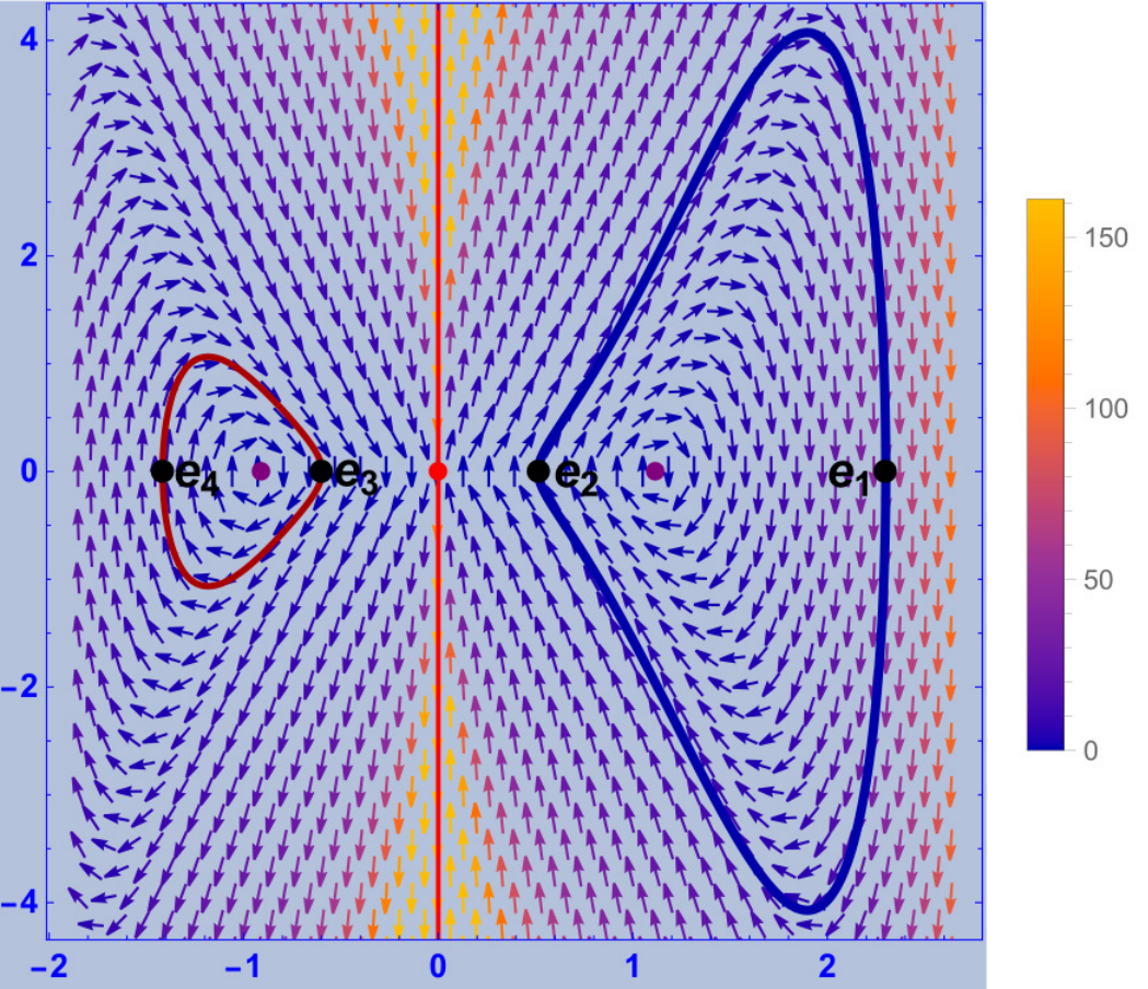

Example 2.6
The picture on the left of Figure 2 depicts the plot of the vector field , , thought of as a vector field defined on minus the -axis. The plot reproduces only the direction of the vector field and the legend specifies the magnitude. The blue and red curves are the reduced phase curves contained in the negative and positive half-planes (dark red) and (blue). The value of the constant is . The origin (the red point) is the isolated singular point of the phase curve. The two points colored in purple are the two zeroes of . The picture on the right of Figure 2 reproduces the corresponding “standard” phase portrait. Figure 3 reproduces phase curves for and (left) and (right). When , the phase curve consists only of a singular point, the origin (in red). When the phase curve consists of two singular points, the origin and , one of the two zeroes of the vector field (in purple). These phase curves are “virtual” in the sense that are not originated from B-strings. When the phase curve has an isolated singular point (the origin) and a smooth reduced phase curve contained in the half-plane (colored in red). When , the phase curve has two singular points, the origin and the other zero of the vector field (colored in black) and a smooth connected component (colored in black) contained in the half-plane . When the phase curve has an isolated singular point (the origin) and two smooth connected components (colored in blue). One contained in the half-plane and the other one in the half-plane .
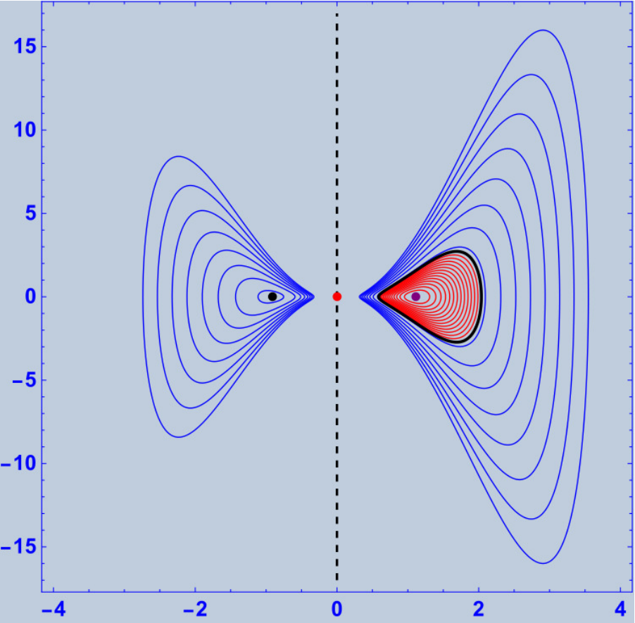
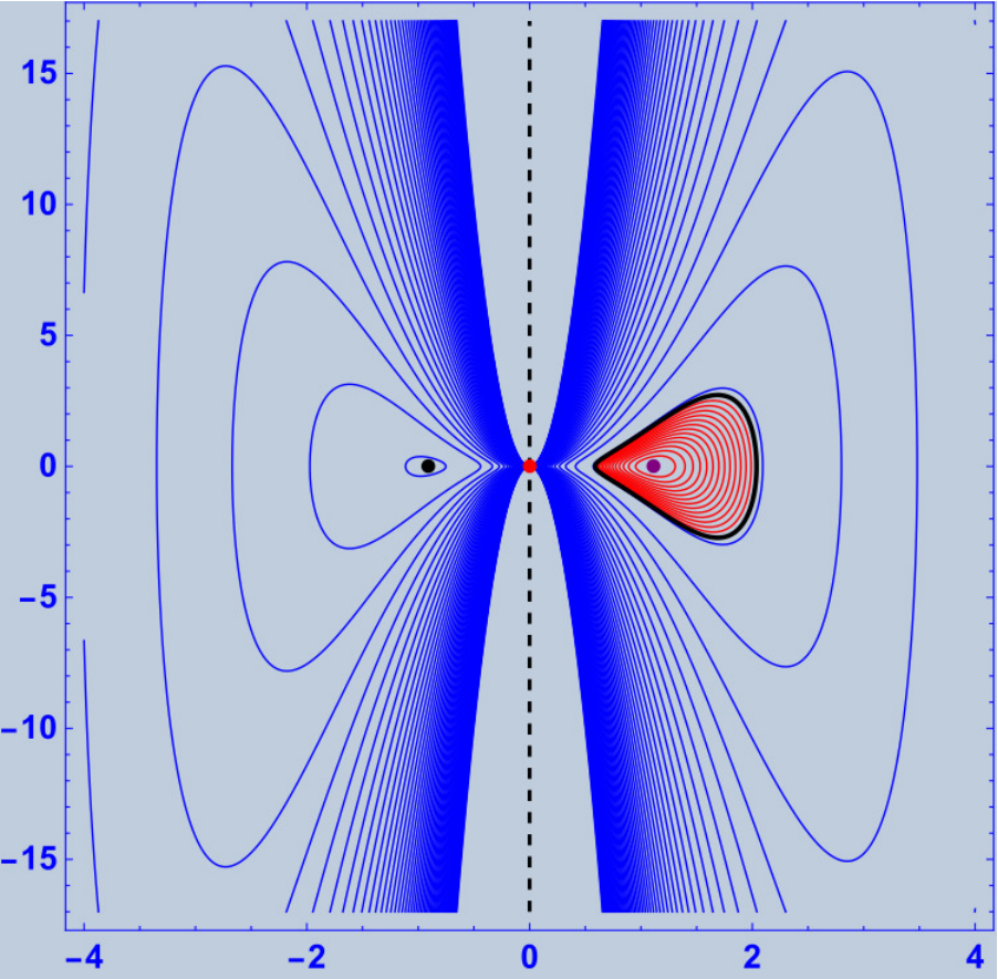
Remark 2.7
Proposition 2.4 proves that, up to equivalence, there exists a one parameter family of B-curves, depending on the constant of integration . It turns out that this constant of integration can be described in terms of the Lagrange multiplier and the largest root of the polynomial . Indeed, as shown above, this polynomial has two positive roots, which we denote by . Then, it follows from that
| (7) |
From this relation we can assume that B-curves depend on and and we can consider these parameters as the fundamental ones. In addition, the -invariant of a critical curve can be built inverting a function involving incomplete elliptic integrals of the third kind, the Jacobi’s amplitude and the Jacobi’s sn-function, with parameters that depend on and . Consequently, also the least period of can be written in terms of complete elliptic integrals of the first and third kind (we refer to the first part of Appendix A for the explicit formulae).
The set of equivalence classes of B-curves is in one-to-one correspondence with the plane domain , where was defined in Remark 2.1 as the only positive solution of .
Theorem 2.8
For every , the map is bijective.
Proof. The proof is a straightforward consequence of the existence and uniqueness of solutions for ordinary differential equations. For each and fixed, we get a unique from (7). Note that for fixed the relation (7) between and is bijective. Then, there exists a unique, up to translation of the arc-length parameter, solution of (4), denoted by . From the Fundamental Theorem for Spherical Curves, this geometric invariant uniquely determines a convex spherical curve , up to rigid motions. In conclusion, the curve is unique, up to equivalence.
In order to treat the B-curves, it is convenient to fix a suitable representative for each equivalence class. Let and be the unique solution of (4) such that , where denotes the least period of . Consider to be the unique B-curve with curvature such that
| (8) |
We call , obtained as above, the standard B-curve with parameters and .
Remark 2.9
It is not restrictive to focus exclusively on standard B-curves and, hence, from now on we implicitly assume that the B-curves in consideration are in their standard form.
We finish this section by formulating the closure condition for a B-curve in terms of the monodromy map. For a B-curve we define the (spherical) Frenet frame field along as the map where denotes the usual vector cross product of . The map is called the monodromy.
Theorem 2.10
The monodromy is a continuous function of and . Moreover, is a B-string if and only if has finite order.
Proof. Let and consider a B-curve (in its standard form). Since is a solution of (4), it also satisfies (2), together with the initial conditions and . Therefore, is a real-analytic function of and , and so is . On the other hand, satisfies
| (9) |
where
and for
Consequently, is also a real-analytic function of and .
The least period of can be written in terms of complete elliptic integrals of the first and third kind (see Part I of Appendix A). It then follows from the properties of these integrals that is a continuous function which is real-analytic on i.e., the complement of the zero locus of the real-analytic function . Thus, is also a continuous function and real-analytic on .
Finally, since is periodic with least period , we conclude from (2) that for every ,
This finishes the proof.
Remark 2.11
Observe that the order of the monodromy is, precisely, the wave number of .
3 Integrability by Quadratures and Existence of B-Strings
In this section we give the parameterization of B-curves in terms of just one quadrature and prove the main theorems of the paper. The parameterization we will obtain in this section is, essentially, the one of Theorem 1.1. Observe that, locally, the ordinary differential equation determining can be used to make a change of variable in and so this parameterization depends on just one quadrature.
We begin by defining a curve in the plane domain . The exceptional locus is the smooth curve defined by the equation
| (10) |
It is easy to check that this exceptional curve is contained in . We say that the parameters are exceptional if they belong to . Moreover, for any , the cubic equation (10) has a unique positive root , which may be explicitly computed. The function is real-analytic and is the graph of (see Figure 7). For convenience, if we will define .
We next introduce some functions which will play an essential role on the parameterization of B-curves. Let be defined by
where is the least period of and is the indicator function of , i.e., is zero everywhere but at the points in which case . We then define the angular function
| (11) |
and the radial and height functions, respectively,
| (12) | |||||
| (13) |
From these definitions, some basic features of these functions can be deduced:
- 1.
The height functions are periodic (with least period ) and even. They have a minimum at and a maximum at . (See Figure 4.)
Figure 4: The graph of the height function for and . In this picture we show the portion of the graph on the interval . - 2.
The radial functions have two different qualitative behaviors depending on whether or not:


Figure 5: The graphs of the radial functions for: and (left); and, and (right). In the left figure we take the portion of the graph on the interval , while in the right one we are showing the graph on the interval . - 3.
The angular functions are arithmetic quasi-periodic (with quasi-period ) and odd. In the interval , possesses an inflection point at with . However, their qualitative behavior depends on whether or :
- (a)
If , in the same interval, has exactly two critical points, an absolute minimum somewhere between and an absolute maximum in . These functions are increasing from the minimum to the maximum and they tend to as . (See Figure 6, Left.)
- (b)
If , then is strictly decreasing and it tends to as . (See Figure 6, Right.)


Figure 6: The graphs of the angular functions for: and (left); and, and (right). The black segment represents the jump of the quasi-periodic function. If the length of the segment is a rational multiple of , the critical curve is periodic (see Theorem 3.3). In this pictures we show the portion of the graph on the interval . - (a)
We have now all the necessary information to prove the parameterization of B-curves (the following result corresponds to Theorem 1.1 in the Introduction).
Theorem 3.1
Let where is defined in Remark 2.1, and be a solution of the Cauchy problem
where is the quartic polynomial defined in (5) and is the least period of . Then, is a positive periodic function. Moreover, define the curve
where , and are the height, radial and angular functions introduced above, (11)-(13). Then, is the B-curve with parameters , in its standard form.
Proof. The first part of the statement was already proven in previous section. It remains to prove that is the B-curve with parameters . For simplicity, we will omit the subscripts and throughout this proof.
We first note that for every the function
is real-analytic. In fact, if is not exceptional, then . Note that is exceptional if and only if and . Thus, in this case
This implies that the angular function is real-analytic. By construction, so is the height function .
We next distinguish between the cases where is exceptional or not.
Suppose first that is not exceptional. Then, as shown above holds and, hence, is a real-analytic spherical curve. Moreover, since , we have
Computing the derivative we get
and . Here we have used the conservation law (4) to simplify above expression. Hence, is an arc-length parameterized spherical curve. Then, computing the second order derivative of , and using the Euler-Lagrange equation (2) and the conservation law (4) to simplify the expression, we obtain that
from which we conclude that the geodesic curvature of is either or . In what follows, we will discard the second case. From above computations we also deduce that
This implies
A straightforward computation yields
and, hence, . That is and is an arc-length parameterized curve with curvature and the same initial conditions of the (standard) B-curve. Consequently, both of them coincide.
Finally, we treat the case where is exceptional. In this case vanishes on and is positive on . By definition,
where .
It is then clear that is continuous and real-analytic away from the discrete set . On the set we can argue as in the non-exceptional case to prove that is an arc-length parameterized spherical curve with and such that
We next prove that is of class on . By construction, , for any , where is a rotation around the -axis. Hence, it suffices to show that is of class at . Note that the first component of is everywhere real-analytic. Since is a real-analytic function, the second and third components of are of class at if and only if the function
is of class at . Recall that and that, in the exceptional case . Thus, is continuous at . Moreover, on the left of we have
where , and are the roots of the polynomial , (5). Therefore,
While, on the right of ,
and so
This implies that
Consequently, is an arc-length parameterized spherical curve of class . Let be the standard B-curve with parameters and . Then, both and are arc-length parameterized spherical curves with the same curvature and the same initial conditions, and . Since is real-analytic and is of class and real-analytic on , we may conclude that .
More precisely, let and be the (spherical) Frenet frame fields along and , respectively. By construction, is continuous and real-analytic on , while is real-analytic everywhere. Then there exists a continuous map such that . On , and are both solutions of the linear system
Thus, is constant on . By continuity, one concludes that is constant everywhere. Moreover, since , we obtain that is the identity. This proves that .
Remark 3.2
A B-curve passes through the pole of the unit-sphere if and only if the parameters are exceptional, i.e., if or, equivalently, if . Moreover, the B-curve passes through the pole, precisely, whenever .
The jump of the B-curve with parameters is defined by
| (14) |
The curve is periodic if and only if is a rational multiple of . (See Figure 6.)
The jump function can be seen as a period map in the following way. Let be the stabilizer of the vector . From Theorem 3.1 it follows that the monodromy map is -valued. Then, since is contractible and is continuous, there exist continuous functions such that
We say that is a period map. The period map is unique and . Keeping in mind that is real-analytic on the open set , that and the integrand are real-analytic on , we deduce that the period maps are real-analytic on .
We now introduce the strictly increasing real-analytic function given by
| (15) |
where is the (unique) positive solution of (3). This function will arise when analyzing the asymptotic behavior of .
We next prove the second main result of the paper, which shows the existence of periodic B-curves, i.e., B-strings (this result corresponds to Theorem 1.2 in the Introduction).
Theorem 3.3
Let . Then, there exists an unbounded countable set such that a B-curve with parameters and is periodic if and only if . In other words, for every there exists a B-string with Lagrange multiplier and monodromy
The rational number is the characteristic number of the B-string.
Proof. In order to show the existence of B-strings, we need to analyze the asymptotic behavior of the jump function (for simplicity, we will omit the subscript )
This is a rather standard integral that can be solved in terms of complete elliptic integrals of the first and third kind (for details, see Appendix A). Moreover, by the properties of these elliptic integrals we obtain that is real-analytic on the following sets:
and (see Figure 7 for the plot of these regions). However, the jump function is not real-analytic on since it has a jump discontinuity on the exceptional locus (see Remark 3.4).
We next obtain the limits of as the parameter approaches the boundaries of its domain, i.e., . The proof of the following limits is just a technical computation involving the decomposition of as the sum of three complete elliptic integrals. For the sake of clarity we simply state the limits here, while we postpone the proof to Appendix A.
We begin with the limit when . In this case, for every we have
where is, precisely, the function introduced in (15). On the other hand, we have the following limits when , depending on the sign of ,
if , and
if .
Finally, let be the period maps such that and . Then, there exists a such that . From above limits, and contains the open interval . This concludes the proof.
As mentioned in the previous proof, the function has a jump discontinuity on , i.e., when . Consequently, it is convenient to regularize this function in order to work with a continuous function. Let us define the regularized jump function by
| (16) |
In terms of , a B-curve with parameters is closed, i.e., a B-string, if and only if , where is a rational number of the type for relatively prime natural numbers . The rational number is the characteristic number of the B-string, while the natural number is its wave number.
From Theorem 3.3 we conclude that for any pair of relatively prime natural numbers and satisfying
there exists a B-string with multiplier and characteristic number .
Remark 3.4
Numerical experiments strongly support the ansatz that the regularized jump function is a real-analytic period map for the -Bernoulli’s bending variational problem. In addition, for every the function is a strictly increasing diffeomorphism. This experimental fact would lead to the following conclusions (which are stronger than those of Theorem 3.3):
- 1.
For every and there exists a unique B-string with multiplier such that . In particular, B-strings with multiplier are in one-to-one correspondence with the countable set .
- 2.
The wave number of is , and hence B-strings are not embedded (see Lemma 3.5 for the number of self-intersection points).
In the last part of this section we will prove Theorem 1.3. We first show a technical lemma regarding the number of points of self-intersection.
Lemma 3.5
Let be a B-string with multiplier and characteristic number . Assume also that . Then,
- 1.
The points and , are simple.
- 2.
If , then possesses, exactly, ordinary double points.
- 3.
If , then possesses, at least, points of self-intersection. The angular function has a unique absolute maximum at such that , and we have three different scenarios:
- (a)
Case . In this case the B-string has exactly ordinary double points.
- (b)
Case for some . In this case the B-string has exactly points of self-intersection.
- (c)
Case for some . In this case the B-string has exactly points of self-intersection.
- (a)
Proof. We begin by proving that the points and , are simple. Since , where is a rotation around the -axis (see previous Theorems 3.1 and 3.3) it suffices to show that and are simple. Consider . We exhibit that, if satisfies , then . The radial function reaches its maximum at , . Hence , for some integer . In addition, . Then, , . On the other hand, . This implies . Since and are relatively prime, we have , . Therefore, . But . Thus, and . Next, consider . The radial function reaches its minimum at , . Thus, if satisfies , then , for some integer . In addition, , mod , ie , . On the other hand, . Then, . Thus, , . Since , the only option is . This proves that .
To prove the other assertions, let and be the integers such that
| (17) |
whose existence is guaranteed because and are relatively prime.
Consider first that . The angular function is strictly decreasing on and while . Thus, for every there exists a unique such that . We are going to prove that, for every , is a multiple point. For this purpose, consider
The height and radial functions are even and periodic, with period . Then, and . Taking into account that is an odd function and using (17) we have
This implies that . It remains to prove that . By contradiction, suppose , then there exists a such that , but this is impossible because . We next prove that the points , and are distinct. Let , then
Since and are relatively prime, is an integer number if and only if is an integer multiple of . On the other hand, it is clear that . Hence, and so . This implies that .
Suppose now that , then . Since is strictly decreasing, we have . On the other hand, is also strictly decreasing on , so , for every .
In conclusion, , for every , and it then follows that the points , , are distinct. This proves that possesses, at least, points of self-intersection.
We finally conclude from the first assertion and from the fact that the angular function is strictly decreasing that the points constructed above are the only multiple points of .
In what follows, we analyze the case . Denote by the absolute minimum and absolute maximum, respectively, of on the closed interval . Then, for every there exists a unique such that . Then, arguing as in the case , we prove that , and are distinct multiple points of . However, contrary to the case , these may not be the only multiple points of since the angular function has a unique absolute maximum at such that , and we have three different scenarios:
- (a)
Case . In this case the B-string has exactly points of self-intersection. These points are the ones constructed above. (See Figure 11 of Subsection 5.4.)
- (b)
Case . In this case the B-string has exactly points of self-intersection. All of them are ordinary double points. The first multiple points are the ones constructed in the proof, while the others arise as the two solutions of the equations with . (See Figure 13 of Subsection 5.6.)
- (c)
Case . In this case the B-string has exactly points of self-intersection. The first are ordinary double points (as in previous case), while the remaining points are points of tangential self-intersection. More precisely, these points are, exactly, , . (See Figure 12 of Subsection 5.5.)
This finishes the proof.
A similar argument may be used to obtain the analogue result for the case , which we state in the following remark.
Remark 3.6
We are now in the right position to prove Theorem 1.3, which we state here in a more technical form.
Theorem 3.7
Let be a B-string with parameters and characteristic number . Then, the following conclusions hold true:
- 1.
The trajectory of is invariant by the group generated by the rotation around the -axis and is contained in the spherical region bounded by the planes and .
- 2.
If , then does not intersect the -axis. Moreover:
- (a)
If , is the linking number with the -axis (equipped with the upward orientation) and possesses, exactly, ordinary double points.
- (b)
If , is the linking number with the -axis (equipped with the upward orientation) and possesses, at least, points of self-intersection.
- (a)
- 3.
If , then intersects the -axis times and the moving point travels counter-clockwise around the -axis (equipped with the upward orientation). Moreover, is the turning number of the plane projection of to the plane .
Proof. The first assertion is trivial. In fact, the stabilizer of the trajectory of a B-string is the subgroup generated by the monodromy, that is the group generated by the rotation of an angle around the -axis. Moreover, from Theorem 3.1, it follows that
where is defined in (13). As customary in our proofs, we are avoiding to write the subscripts and , for simplicity in the expressions. Since , the trajectory of the curve is clearly contained in . Similarly, since , from the definition of , one also concludes that the trajectory of the curve lies in the spherical region bounded by the planes of the statement.
Suppose now that . In this case, the radial function defined in (12) is strictly positive and so the linking number is the winding number of around the origin, that is, the degree of the circle map
which is equal to
If , we have and, if , . This proves the second statement (the number of points of self-intersection follows from Lemma 3.5).
Finally, suppose that , then passes through the pole if and only if is a zero of the radial function . In other words, if and only if, . This implies that crosses the -axis when , i.e., times.
Recall that in this exceptional case
where is the characteristic number of , and we denote by . The plane projection of is the “polar” curve
The radial and angular functions satisfy and . Thus, if and is an odd integer, the least period of is , while if and is even, the least period of is . Similarly, if is odd, . Let and be the unit tangent and unit normal vector fields along . Then
This implies that
| (18) |
where is the continuous determination of such that . Considering the properties of the radial and angular functions, possesses jump discontinuities at the points , , and is real-analytic elsewhere. At the points of discontinuity we have
Consequently, is a quasi-periodic function with quasi-period such that . Then, we deduce the following properties from (18):
- 1.
If and is an odd integer, then , and ()
- 2.
If and is an even integer, then , and ()
- 3.
If is an odd integer, , and ()
This proves that the total curvature, i.e., the turning number of is , as claimed.
Remark 3.8
Theorem 3.7 implies that the geometry of a B-string is encoded by its projection onto an annular region (disc-type region if the B-string intersects the -axis) of the oriented plane through the origin and orthogonal to the symmetry axis. The multiple points of the B-string are projected onto the multiple points of the projected plane curve and, vice-versa, each multiple point of the projection gives rise to a multiple point of the string.
If , the projection is counter-clockwise oriented, while if is clockwise oriented. Its symmetry group is the same than the one of the B-string. If , the linking number of the string is the homotopy class of the projection, viewed as a plane curve of the annular region.
4 Theoretical Aspects
In this section we comment on the theoretical aspects behind Theorems 3.1, 3.3 and 3.7 and on the rich “hidden” geometry surrounding the -Bernoulli’s bending variational problem, which is typical of variational problems related to non-commutative completely integrable Hamiltonian contact systems ([25, 26, 29, 30, 37, 54]) and to Liouville integrable geometric variational problems ([41]).
4.1 The Phase Space
Let
be the Maurer-Cartan form of . Then, is a basis for the space of left-invariant -forms. Using the algorithmic procedure illustrated in [29, 31], the momentum space of the functional is the -dimensional submanifold of defined by the embedding
The restriction of the Liouville form of to is the -form
The -form has maximal rank and its characteristic line bundle is generated by the vector field
where is the trivialization of dual to the coframe . The integral curves of are the canonical lifts of the B-curves (not necessarily in their standard form) with multiplier , that is curves of the following type
where is an arc-length parameterized B-curve with multiplier , curvature and where is the derivative of with respect to the arc-length parameter. Thus, the problem has been reduced to the integration of the characteristic vector field of the -invariant -form .
4.2 The Moment Map
The moment map for the -action on is the restriction of the moment map for the -action on equipped with its standard symplectic form. So, we get
where
Using the Killing form we identify with , which is isomorphic to equipped with the Lie algebra structure defined by the usual vector cross product. Modulo these identifications, the moment map can be written as
By construction, is constant along the integral curves of . This implies that if is a B-curve with multiplier and parameter , then
is constant. Note that , where is the constant of integration defined in (7). The oriented line passing through the origin and parallel to is the axis of symmetry of . The element is the momentum of the B-curve and so the constant of integration is the length of the momentum. Identifying with and letting be the corresponding fundamental vector field of , then is the sum of the (adapted) Killing vector fields along which arise in the Lagrangian approach ([42]).
The momentum map has maximal rank at each point of and its image is the open set
where is defined in Remark 2.1.
If , the quartic polynomial
possesses exactly two distinct positive real roots, . The integral curves of with momentum are, precisely, the canonical lifts of B-curves with multiplier and parameter .
The (reduced) phase curve of is the connected component of the singular algebraic curve
contained in the half-plane . It turns out that is a smooth curve and is the affine part of a singular algebraic curve of . Such a curve is, in general, elliptic and it is rational if and only if either or and .
4.3 The Marsden-Weinstein Reduction and the Arnold Connection
Let . The (Marsden-Weinstein) reduced space of is the -dimensional torus . This torus is invariant by the action of the stabilizer and the vector field is tangent to .
The map is -invariant and gives, on , the structure of a principal circle bundle. The line bundle of spanned by defines a connection on the principal bundle .
4.4 Closure Conditions and Integrability by Quadratures
Let be the largest positive root of . Then, . Let be the (discrete) holonomy group of the connection, with reference point . We have that is isomorphic to the monodromy of a B-curve with multiplier and parameter . From a theoretical point of view, the closure condition for a critical curve can be rephrased as follows.
Remark 4.1
A B-curve with momentum is periodic if and only if is finite.
Let be a positively oriented orthogonal basis such that
and be the holonomy bundle of the connection passing through . Then:
- 1.
The map is a covering map with deck transformation group .
- 2.
If is finite, . Otherwise, .
- 3.
The set is an integral curve of and, hence, is a B-curve with multiplier and momentum .
We next explain how to find the parameterization of a B-curve given in Theorem 3.1. Let and
Assume that is a (periodic) solution to the Cauchy problem
We denote by the parameterization of the phase curve. Choose any cross section of . This amounts to find satisfying
Such a map can be easily found by elementary linear algebra. For instance,
satisfies above equation. Clearly, any other cross section is of the form
Parallel sections of the connection are solutions of
It follows from the expression of and , that is, precisely, a parallel section if and only if
Hence, the map is a parallel cross section and is the standard configuration of a B-curve with parameters exhibited in Theorem 3.1.
Let and (which is a countable set containing ). The function is a strictly increasing real-analytic diffeomorphism of onto where
Then, we may choose as a fundamental parameter and express and as functions of . Let be defined by (if , then , while if , we set ). Note that there exist countably many such that .
Remark 4.2
With this notation the results of Theorems 3.3 and 3.7 can be reformulated as follows:
- 1.
An arc-length parameterized curve is a B-string with multiplier if and only if
is constant and .
- 2.
For every such that , there exists a B-string with momentum . Two B-strings are equivalent if and only if their momenta have the same length.
- 3.
Let . Then, the stabilizer of a B-string with momentum is generated by the rotation around of an angle . Moreover:
- (a)
If , is the linking number of the B-string with the oriented axis . In this case, the B-string possesses, exactly, ordinary double points.
- (b)
If , the B-string turns counter-clockwise around and intersects this axis times. The turning number of the plane projection of the B-string to the oriented plane through the origin and orthogonal to is .
- (c)
If , is the linking number of the B-string with the axis . In this case, the B-string possesses, at least, points of self-intersection. (See Lemma 3.5 for more details about the intersection points.)
- (a)
Remark 4.3
Assuming the ansatz that is strictly increasing, then and, for every there exists a unique equivalence class of B-strings with multiplier such that .
5 Examples
In this section we will consider several examples which illustrate all the theoretical findings of previous sections.
5.1 Case :
In this example we consider a B-string with multiplier and characteristic number ( and ). Since the B-string is of negative type (i.e., ).
According to Theorems 3.3 and 3.7, the B-string has a counter-clockwise five-fold symmetry; its linking number with the (upward oriented) -axis is (which coincides with the winding number and the turning number of the plane projection), and it possesses ordinary double points. In Figure 8, we show the corresponding B-string, its plane projection and its associated phase curve, where we illustrate these properties.

5.2 Case (without ordinary double points):
In this example we consider an exceptional B-string with multiplier and characteristic number ( and ).
Observe in Figure 9 that, as stated in Theorems 3.3 and 3.7, the B-string possesses a counter-clockwise nine-fold symmetry, the turning number of the plane projection is and that it possesses a multiple point (at the pole ) of multiplicity . Observe that the largest natural number relatively prime with and such that is and so, we conclude from Remark 3.6, that this B-string has ordinary double points.

5.3 Case (with ordinary double points):
In this example we consider an exceptional B-string with multiplier and characteristic number ( and ).
In Figure 10 we can see that, as stated in Theorems 3.3 and 3.7, the B-string possesses a counter-clockwise nine-fold symmetry, the turning number of the plane projection is and that it possesses a multiple point (at the pole ) of multiplicity . Moreover, the B-string also possesses ordinary double points, since in this case the largest natural number relatively prime with and such that is (see Remark 3.6).

5.4 Case (with ordinary double points):
In this example we consider a B-string of positive type with multiplier and characteristic number ( and ). By positive type, we mean that holds.
Observe in Figure 11 that, as stated in Theorems 3.3 and 3.7, the B-string possesses a clockwise eight-fold symmetry, the winding number (also, the turning number) of the plane projection is and it possesses ordinary double points.

5.5 Case (with tangential double points):
In this example we consider a B-string of positive type with multiplier and characteristic number ( and ).
This B-string possesses a clockwise eleven-fold symmetry, the winding number (also, the turning number) of the plane projection is and it possesses ordinary double points and points of tangential self-intersection.

5.6 Case (with ordinary double points):
In this example we consider a B-string of positive type with multiplier and characteristic number ( and ).
Observe in Figure 13 that, as stated in Theorems 3.3 and 3.7, the B-string possesses a clockwise nine-fold symmetry, the winding number (also, the turning number) of the plane projection is and that it possesses ordinary double points, since .

Appendix A. The curvature of the Extrema and the Complete Elliptic Integral
This appendix has two parts. In the first one we will show how to build the -invariant from incomplete elliptic integrals of the third kind and how to compute its least period in terms of complete elliptic integrals. In the second part we will decompose the integral and compute its limits as approaches the boundaries of its domain.
Part I: The Curvature of the Extrema
Let and be the Legendre’s incomplete elliptic integrals of the first and third kind, defined as
and , be the corresponding complete elliptic integrals. Let be the Jacobi’s amplitude with parameter and the associated Jacobi’s elliptic function. For simplicity, we denote by
and
where and are the roots of the polynomial . Recall that and are functions of the fundamental parameters and . Let be the solution of (4) with and be its least period. By construction, is strictly increasing on and . Let be defined by
Then, from (4) it follows that . Since is even, this is enough to reconstruct on the whole real axis. Using and of [10], we obtain
where
Putting , we see that the least period of is
Figure 14 reproduces the graphs of the -function and of the -function on the intervals and , when , , , . The -function is evaluated via the Mathematica library of elliptic functions while the function is evaluated solving numerically (2) with initial conditions and . The black-dashed portion of the graph of on is obtained by symmetrizing the graph of with respect to the bisector of the first quadrant, showing that the two methods are in agreement with each other.


The -Bernoulli’s bending energy of a B-string can also be evaluated in terms of the wave number and complete elliptic integrals of the first kind as
Part II: The Complete Elliptic Integral
Using (4) to make a change of variable in the definition of , (14), we have
This integral can be solved in terms of complete elliptic integrals of the first and third kind.
For simplicity, we denote by
We then have
where is the indicator function of the exceptional locus and,
| (19) | |||||
| (20) | |||||
| (21) |
These formulas follow from three standard elliptic integrals. The first one (cf. 340.01 and 341.03 of [10]) is
The second elliptic integral (cf. 257 and 259 of [10]) is
where and are as above. The third relevant elliptic integral (cf. 257.39 and 259.04 of [10]) is
where , , and are as above, and
We begin proving that when approaches from the right. By construction we have that too, and, hence, it follows that
and
We now see that the coefficients in (19)-(21) tend to, respectively,
while
and
Finally, recalling that , using the above limits and (15) we conclude that
| (22) |
In what follows, we prove the limit when . This limit will depend on the sign of . More precisely, we will see that
and
In order to prove these limits we observe that, as , the following asymptotic estimates hold true:
and
| (23) |
Moreover, recall that as and so, in our case, we have
as . Combining this and the above estimates we conclude that
as . This proves the first limit.
For the other limits we need some basic properties of the complete elliptic integral of the third kind . Let and consider the function
This function is bounded below by and above by . In addition, for every and when , for every value of . Moreover, for every ,
where is the complete elliptic integral of the second kind. From this we infer that
From these properties we deduce the following facts:
- 1.
If is a smooth curve such that when and is an asymptote of as , then
- 2.
If is a smooth curve such that when and is an asymptote of as , then
Combining both things, it follows that as ,
In view of these properties, fix sufficiently large and consider the curves
From above estimates when , we have the following asymptotic behavior for ,
while for , it depends on the value of ,
Thus, and is an asymptote of as . Similarly, as . Hence, it follows from above facts that
when .
It is then clear, combining this and above estimates, that
This completes the proof about the claimed limits for when .
Appendix B. Closed -Elasticae in the Plane
We briefly comment about -elasticae in in order to clarify some assertions made in the Introduction. We begin with the non-existence of closed convex -elasticae other than circles. In the phase curves for convex -elasticae are the singular rational curves (see the picture on the left of Figure 16)
where . Then, following the general argument of the Introduction, is a solution of and is a periodic, regular parameterization of the smooth component of the phase curve lying in the positive half-plane .


Integrating by quadratures, the arc-length parameterization of a critical curve, up to rigid motions, is
Let be the least period of . Then,
On the other hand,
and
Hence
This implies that the trajectory of is invariant by the subgroup generated by a non-trivial translation along the -axis. In particular, it is unbounded.


Next we focus on the non-existence of non-convex critical curves with periodic curvature. In this case . By contradiction, suppose that is periodic and non-constant. Without loss of generality . Let , be the connected component of containing the origin. Since is not strictly positive, at least one among or is finite. Put . Then, is a parameterization of an open arc contained in (see the picture on the right of Figure 15; is represented in the black part). By construction, and, in addition, there exist such that on and on . Taking into account that is a solution of the Euler-Lagrange equation, is an integral curve of the vector field
Thus, cannot invert his motion along . Since is homeomorphic to , this implies that is a homeomorphism onto its image. Therefore, intersects the -axis at one point, namely at . Hence, on and on . Let and be the inverses of and respectively (see the picture on the left of Figure 16; the graph of is shown in black while the graph of in red). Then,
Consequently, can be extended to a function attaining its maximum at , strictly increasing on and strictly decreasing on (see the picture on the right of Figure 16) such that
This implies and , which is a contradiction.
Acknowledgements
The first author is partially supported by PRIN 2017 “Real and Complex Manifolds: Topology, Geometry and Holomorphic Dynamics” (protocollo 2017JZ2SW5-004) and by the GNSAGA of INDAM. The present research was also partially supported by MIUR grant “Dipartimenti di Eccellenza” 20182022, CUP: E11G18000350001, DISMA, Politecnico di Torino.
The authors would like to thank the referees for their valuable comments which have helped to improve the manuscript.
References
- [1]
- [2] J. Arroyo, M. Barros and O. J. Garay, Willmore-Chen Tubes on Homogeneous Spaces in Warped Product Spaces, Pac. J. Math. 188-2 (1999), 201–207.
- [3] J. Arroyo, O. J. Garay and J. J. Mencía, Closed Generalized Elastic Curves in , J. Geom. Phys. 48-2 (2003), 339–353.
- [4] J. Arroyo, O. J. Garay and A. Pámpano, Constant Mean Curvature Invariant Surfaces and Extremals of Curvature Energies, J. Math. Anal. App. 462 (2018), 1644–1668.
- [5] J. Arroyo, O. J. Garay and A. Pámpano, Delaunay Surfaces in , Filomat 33-4 (2019), 1191–1200.
- [6] M. Barros, A. Ferrández and P. Lucas, Conformal Tension in String Theories and M-Theory, Nuclear Phys. B 584 (2000), 719–748.
- [7] M. Barros, A. Ferrández, P. Lucas and M. A. Meroño, Willmore Tori and Willmore-Chen Submanifolds in Pseudo-Riemannian Spaces, J. Geom. Phys. 28 (1998), 45–66.
- [8] J. Bernoulli, Curvatura Laminae Elasticae, Acta Eruditorum Lipsiae (1694), 262–276.
- [9] W. Blaschke, Vorlesungen uber Differentialgeometrie und Geometrische Grundlagen von Einsteins Relativitatstheorie I-II: Elementare Differenntialgeometrie, Springer, (1921-1923).
- [10] P. F. Byrd and M. D. Friedman, Handbook of Elliptic Integrals for Engineers and Physicists, Springer-Verlag, Berlin, Gottingen, Heidelberg, (1954).
- [11] C. Bohle, G. P. Peters and U. Pinkall, Constrained Willmore Surfaces, Calc. Var. Partial Differential Equations 32 (2008), 263–277.
- [12] E. Calabi, P. J. Olver and A. Tannenbaum, Affine Geometry, Curve Flows, and Invariant Numerical Approximations, Adv. Math. 124 (1996), 154–196.
- [13] A. Calini and T. Ivey, Integrable Geometric Flows for Curves in the Pseudoconformal , J. Geom. Phys. 166 (2021), 104249.
- [14] A. Calini, T. Ivey and G. Marí-Beffa, Remarks on KdV-type Flows on Star-Shaped Curves, Phys. D 238-8 (2009) 788–797.
- [15] A. Calini, T. Ivey and G. Marí-Beffa, Integrable Flows for Starlike Curves in Centroaffine Space, SIGMA 9 (2013), 022.
- [16] P. B. Canham, The Minimum Energy of Bending as a Possible Explanation of the Biconcave Shape of the Human Red Blood Cell, J. Theor. Biol. 26-1 (1970), 61–76.
- [17] R. Capovilla, J. Guven and E. Rojas, Hamilton’s Equations for a Fluid Membrane: Axial Symmetry, J. Phys. A: Math. Gen. 38 (2005), 8201–10.
- [18] J. Cho, M. Pember and G. Szewieczek, Constrained Elastic Curves and Surfaces with Spherical Curvature Lines, arXiv: 2104.11058 [math.DG], (2021).
- [19] K. S. Chou and C. Qu, The KdV Equation and Motion of Plane Curves, J. Phys. Soc. Japan 70 (2001), 1912–1916.
- [20] K. S. Chou and C. Qu, Integrable Equations Arising from Motions of Plane Curves, Phys. D 162 (2002), 9–33.
- [21] K. S. Chou and C. Qu, Integrable Equations Arising from Motions of Plane Curves II, J. Nonlinear Sci. 13-5 (2003), 487–517.
- [22] L. Euler, De curvis elasticis. In: Methodus Inveniendi Lineas Curvas Maximi Minimive Propietate Gaudentes, Sive Solutio Problematis Isoperimetrici Lattissimo Sensu Accepti, Additamentum 1 Ser. 1, Vol. 24, Lausanne, (1744).
- [23] E. Evans, Bending Resistance and Chemically Induced Moments in Membrane Bilayers, Biophys. J. 14 (1974), 923–931.
- [24] T. Flash and A. A. Handzel, Affine Differential Geometry Analysis of Human Arm Movements, Biol. Cybern. 96-6 (2007), 577–601.
- [25] A. T. Fomenko and V. V. Trofimov, Geometric and Algebraic Mechanisms of the Integrability of Hamiltonian Systems on Homogeneous Spaces and Lie Algebras, Dinamical Systems, Vol. 7 Springer-Verlag, (1994).
- [26] H. Goldschmidt and S. Sternberg, The Hamilton-Cartan Formalism in the Calculus of Variations, Ann. Inst. Fourier 23 (1973), 203–267.
- [27] R. E. Goldstein and D. M. Petrich, The Korteweg-de Vries Hierarchy as Dynamics of Closed Curves in the Plane, Phys. Rev. Lett. 67 (1991), 3203.
- [28] R. E. Goldstein and D. M. Petrich, Solitons, Euler’ s Equation and Vortex Patch Dynamics, Phys. Rev. Lett. 69 (1992), 555.
- [29] J. D. E. Grant and E. Musso, Coisotropic Variational Problems, J. Geom. Phys. 50 (2004), 303–338.
- [30] V. Guillemin and S.Sternberg, Symplectic Techniques in Physics, Cambridge University Press, Cambridge, (1990).
- [31] P. A. Griffiths, Exterior Differential Systems and the Calculus of Variations, Progress in Mathematics, vol. 25, Boston, Birkhauser, (1982).
- [32] H. Hasimoto, A Soliton on a Vortex Filament, J. Fluid Mech. 51 (1972), 477–485.
- [33] H. Hasimoto, Motion of a Vortex Filament and its Relation to Elastica, J. Phy. Soc. Japan 31 (1971), 293–294.
- [34] W. Helfrich, Elastic Properties of Lipid Bilayers: Theory and Possible Experiments, Z. Natur. C 28 (1973), 693–703.
- [35] L. Hsu, Calculus of Variations via the Griffiths Formalism, J. Differential Geom. 36 (1992), 551–589.
- [36] G. Jensen, E. Musso and L. Nicolodi, The Geometric Cauchy Problem for the Membrane Shape Equation, J. Phys. A: Math. Theor. 47 (2014), 495201.
- [37] B. Jovanovic, Noncommutative Integrability and Action-Angle Variables in Contact Geometry, J. Symplectic Geom. 10-4 (2012), 535–561.
- [38] S. Kida, A Vortex Filament Moving without Changing of Form, J. Fluid Mech. 112 (1981), 397–409.
- [39] J. Langer and R. Perline, Curve Motion Inducing Modified Korteweg-de Vries Systems, Phys. Lett. A 239 (1998), 36–40.
- [40] J. Langer and R. Perline, Poisson Geometry of the Filament Equation, J. Nonlinear Sci. 1 (1991), 71–93.
- [41] J. Langer and D. A. Singer, Liouville Integrability of Geometric Variational Problems, Comment. Math. Helv. 69 (1994), 272–280.
- [42] J. Langer and D. A. Singer, The Total Squared Curvature of Closed Curves, J. Diff. Geom. 20 (1984), 1–22.
- [43] R. Levien, The Elastica: A Mathematical History, Technical Report No. UCB/EECS-2008-103, University of Berkeley.
- [44] R. López and A. Pámpano, Stationary Soap Films with Vertical Potentials, Nonlinear Anal. 215 (2022), 112661.
- [45] T. Miura and K. Yoshizawa, Complete Classification of Planar p-Elasticae, ArXiv: 2203.08535 [math.AP], (2022).
- [46] S. Montaldo, C. Oniciuc and A. Pámpano, Closed Biconservative Hypersurfaces in Spheres, J. Math. Anal. Appl. (2022), 126697.
- [47] S. Montaldo and A. Pámpano, On the Existence of Closed Biconservative Surfaces in Space Forms, to appear in Comm. Anal. Geom.
- [48] E. Musso, Variational Problems for Plane Curves in Centro Affine Geometry, J. Phys A: Math. Theor. 43 (2010), 1751–8113.
- [49] E. Musso, Congruence Curves of the Goldstein-Petrich Flows, Harmonic maps and Differential Geometry, Contemp. Math. Vol 542, Providence, 99–113, (2011).
- [50] E. Musso, Motions of Curves in the Projective Plane Inducing the Kaup-Kupershmidt Hierarchy, SIGMA 8 (2012), 030.
- [51] E. Musso and L. Nicolodi, Hamiltonian Flows on Null Curves, Nonlinearity 23 (2010), 2117.
- [52] E. Musso and F. Salis, The Cauchy-Riemann Strain Functional for Legendrian Curves in the 3-Sphere, Ann. Mat. Pura Appl. 199 (2020), 2395–2434.
- [53] K. Nakayama, H. Segur and M. Wadati, Integrability and the Motion of Curves, Phys. Rev. Lett. 69 (1992), 2603.
- [54] P. Ortega and T. Ratiu, Moment Maps and Hamiltonian Reductions, Progress in Mathematics, 222, Boston, Birkhauser, (2004).
- [55] A. Pámpano, Critical Tori for Mean Curvature Energies in Killing Submersions, Nonlinear Anal. 200 (2020), 112092.
- [56] U. Pinkall, Hopf Tori in , Invent. Math. 81 (1985), 379–386.
- [57] U. Pinkall, Hamiltonian Flows on the Space of Star-Shaped Curves, Results Math. 27 (1995), 328–332.
- [58] D. Raviv and R. Kimmel, Affine Invariant Geometry for Non-Rigid Shapes, Int. J. Comput. Vis. 111-1 (2015), 1–11.
- [59] Y. Soliman, A. Chern, O. Diamanti, F. Knoppel, U. Pinkall and P. Schroeder, Constrained Willmore Surfaces, ACM Trans. Graph. 40-4 (2021), 112.
- [60] C. Truesdell, The Rational Mechanics of Flexible or Elastic Bodies: 1638–1788, Leonhard Euler, Opera Omnia, Birkhauser, (1960).
- [61] Z. C. Tu and Z. C. Ou-Yang, A Geometric Theory on the Elasticity of Bio-Membranes, J. Phys. A: Math. Gen. 37 (2004), 11407.
- [62] S. Verpoort, Curvature Functionals for Curves in the Equi-Affine Plane, Czechoslov. Math. J. 61 (2011), 419–435.
- [63] V. M. Vassilev, P. A. Djondjorov and I. M. Mladenov, Cylindrical Equilibrium Shapes of Fluid Membranes, J. Phys. A: Math. Theor. 41 (2008), 435201.
- [64]
Emilio MUSSO
Dipartimento di Scienze Matematiche (Department of Mathematical Sciences) - Politecnico di Torino, Corso Duca degli Abruzzi 24, I-10129 Torino, Italy
E-mail: emilio.musso@polito.it
Álvaro PÁMPANO
Department of Mathematics and Statistics, Texas Tech University, Lubbock, TX, 79409, USA
E-mail: alvaro.pampano@ttu.edu