On Polynomially Solvable Constrained Input Selections
for Fixed and Switched Linear Structured SystemsJournal: Elsevier
Abstract
This paper investigates two related optimal input selection problems for fixed (non-switched) and switched structured systems. More precisely, we consider selecting the minimum cost of inputs from a prior set of inputs, and selecting the inputs of the smallest possible cost with a bound on their cardinality, all to ensure system structural controllability. Those problems have attracted much attention recently; unfortunately, they are NP-hard in general. In this paper, it is found that, if the input structure satisfies certain ‘regularizations’, which are characterized by the proposed restricted total unimodulairty notion, those problems can be solvable in polynomial time via linear programming (LP) relaxations. Particularly, the obtained characterizations depend only on the incidence matrix relating the inputs and the source strongly connected components (SCC) of the system structure, irrespective of how the inputs actuate states within the same SCC. They cover all the currently known polynomially solvable cases (such as the dedicated input case), and contain many new cases unexploited in the past, among which the source-SCC separated input (SSSI) constraint is highlighted. Further, for switched systems, the obtained polynomially solvable condition (namely the joint SSSI constraint) does not require each of the subsystems to satisfy the SSSI constraint. We achieve these by first formulating those problems as equivalent integer linear programmings (ILPs), and then proving total unimodularity of the corresponding constraint matrices. This property allows us to solve those ILPs efficiently via LP-relaxation. We also discuss solutions obtained via LP-relaxation and LP-rounding in the general case. Several examples are given to illustrate the obtained theoretical results.
Keywords:
Structural controllability, input selection, switched system, linear programming, total unimodularity1 Introduction
Over the past decade, input/output (I/O) selections for a large-scale dynamic system to achieve certain performances have received considerable attention [1, 2, 3, 4]. Examples include estimation error minimization of the Kalman filter by sensor placement [5], stabilization by joint I/O selection and feedback design [6], achieving various performances related to controllability/observability [2, 3, 4, 7], etc. This paper is about I/O selections for controllability.
Broadly speaking, problems concerning I/O selections for controllability can be divided into two categories. The first one is selecting inputs to optimize some control energy-related metrics, such as the trace, determinant, or inverse of the minimum eigenvalue of the controllability Gramian [3, 4, 8]. One typical approach to some of those problems is exploiting the modular, submodular, or weak submodular structure of the corresponding optimization problems, which often leads to greedy algorithms with provable approximation guarantees [3]. The second one is to design certain ‘sparse’ inputs for ensuring controllability in the qualitative sense. Depending on what qualitative notion is adopted, this category can also be divided into two subclasses. When the purpose is to ensure controllability in the numerical sense, the minimum number of inputs needed has an analytical expression (i.e., being the maximum geometric multiplicity of the system state transition matrix) [9]. However, if the available input vectors are given a priori, this problem turns out to be NP-hard [2]. The other subclass is about structural controllability, an alternative notion of controllability in the generic sense [10], detailed as follows.
The problems of optimally selecting inputs to achieve structural controllability can be roughly classified into two classes, depending on the objectives. The first class of problems aims at determining the minimum number/cost of input links (typically, the sparsest input matrices) for structural controllability. When there is no constraint on the structure of the input configuration or all the available inputs are dedicated (i.e., each input can actuate at most one state variable), it has been shown that these problems can be solved in polynomial time by transforming them to some maximum matching problems [11, 12]. Recently, [13] extends the dedicated input constraint to the so-called source strongly-connected component (SCC) grouped constraint and shows that if the available inputs satisfy this constraint, then the aforementioned problems are polynomially solvable. Further, [14] shows that finding the sparsest interconnection structure (both among states and between inputs and states) for a system to be structurally controllable is NP-hard, if the available interconnections among states are given a priori.
The second class of problems intends to find the minimum number/cost of inputs (typically, the input matrices with the smallest number of columns) to achieve structural controllability. Note that compared to the first class of problems, selecting an input indicates all the input links incident to this input are selected simultaneously. It has been shown this problem has an analytical solution if there is no constraint on the input structure [1]. However, if the available inputs are given a priori (called the constrained input selection problem in this case), this problem is generally NP-hard [15]. Due to the NP-hardness, only very limited scenarios are known for this problem to be polynomially solvable, such as the dedicated input case in [11, 12]. For approximation, [15] reduces this problem to the set-cover problem for a special case, and [16] gives a flow-network based approximation algorithm.
In this paper, we advance the state of the art in searching polynomially solvable conditions for constrained input selection problems. More precisely, in addition to considering the problem of selecting the minimum cost of inputs from a given set to achieve system structural controllability, we also reinvestigate this problem by imposing an upper bound on the number of selected inputs. To our knowledge, no polynomial-time algorithms have been reported for these problems in the non-dedicated input case, except for some trivial cases (c.f., the system structure is strongly-connected). The initial idea of our study is that, since the addressed problems are NP-hard due to the fact that determining the minimum number of inputs to achieve input-reachability is NP-hard [15] (see also Section 3) , what happens for the class of systems where the latter problem is no longer intractable?
Main contributions: Starting from this point, we reveal if the input structure satisfies the so-called source-SCC separated input constraint (SSSI constraint), i.e., no inputs can actuate two different source-SCCs simultaneously, the addressed input selection problems can be solved in polynomial time. We further generalize this result, showing that if the input structure satisfies certain ‘regularizations’, which are characterized by the restricted total unimodularity (TU) notion introduced in this paper, those problems are polynomially solvable. The obtained conditions largely extend the currently known polynomially solvable ones, as they depend only on the connections between the inputs and the source-SCCs of the system structure, but irrespective of how each input actuates states within the same SCC. Those results are further extended to the switched systems for similar input selection problems. Particularly, a joint SSSI constraint is proposed, which does not require each subsystem to meet the SSSI constraint but preserves the polynomial solvability. Key to our results is first formulating the constrained input selection problems as equivalent integer linear programming (ILP) problems, and then proving that the corresponding constraint matrices are TU under the addressed conditions. This allows us to solve those ILPs efficiently by simply solving their linear programming (LP) relaxations. In this way, we provide an LP-based method for these problems with polynomial time complexity, conceptually different from the graph-theoretic ones. For the general case, we study solutions obtained via LP-relaxation and LP-rounding, resulting in some lower and upper bounds for the minimum cost input selection problem. In particular, the lower bound is tighter than the one obtained via the graph-theoretic method, while the upper bound has a provable approximation factor for a special case. We remark that the LP-based method has also been used in [13] for solving a different input selection problem from this paper. Relative to [13], the considered problems here are essentially NP-hard and more intricate as the set cover problem is embedded. The obtained polynomial solvability conditions are also wider than that in [13]. Partial results of this paper are scheduled to appear in [17]. While [17] only covers the SSSI constraint without proofs, this paper generalizes it to the restricted TU condition, provides the full proofs, and presents extensions to the switched systems as well as solutions in the general case.
The rest of this paper is organized as follows. Section 2 gives the problem formulations, and Section 3 provides some preliminaries in graph theory and structured systems. Section 4 gives the ILP formulations of the considered problems, while Section 5 presents the polynomially solvable conditions for the fixed (non-switched) systems. Solutions in the general case via LP-relaxation and LP-rounding are discussed in Section 6. Extensions to the switched systems are given in Section 7. Section 8 provides two illustrative examples. The last section concludes this paper.
Throughout this paper, for two vectors and , means entry-wisely. A vector is integral if every element is an integer. For an optimization problem , is called the feasible region, is called a feasible solution, the minimum of the objective on is called the optimal (objective) value, or optimum, while the for which the optimum is attained is an optimal solution. () denotes the matrix with all entries (). The set of positive integers is denoted as .
2 Problem formulations
Consider a linear-time invariant system as
| (1) |
in which , are the state variables and inputs, and , .
A structured matrix is a matrix with entries being either fixed zero or a free parameter. Denote the set of structured matrices by , where represents the free parameters. Let and be two structured matrices specifying the sparsity patterns of and , i.e., implies , and implies . In this way, is called a realization of .
Definition 1
[18] is said to be structurally controllable, if there is a realization of it that is controllable.
Controllability of system (1) is a generic property in the sense that, if is structurally controllable, then almost all of its realizations are controllable; otherwise, none is controllable [19]. Given and , let be the sub-matrix of consisting of columns indexed by . Assign a non-negative rational cost to each column of , representing the cost of activating the th input. We say is dedicated, if each column of has at most one nonzero entry. With the notations above, we first consider the following optimal input selection problem:
Problem : minimum cost input selection
| () |
That is, seeks to select the inputs from the prior input matrix with the minimum total cost to achieve structural controllability. Next, we consider the following problem by adding a cardinality upper bound to the number of inputs:
Problem : cardinality-constrained minimum cost input selection
| () |
In other words, intends to select the inputs with a bound on their cardinality and with the total cost as small as possible to ensure structural controllability. It may happen that the optimal solution to , denoted by , has a much larger cardinality than that to . Therefore, may be desirable, for example, when the activation of new inputs may be more expensive compared to increasing the input costs. Throughout this paper, without losing any generality, the following assumption is adopted, which is necessary for the feasibility of and .
Assumption 1
is structurally controllable.
Remark 1
A related problem to is selecting the set of inputs to achieve structural controllability with the smallest possible cost, meanwhile the cardinality is no more than any number of inputs ensuring system structural controllability, i.e., in equals the optimum of with unit input cost (i.e, ; denote this value by ). This problem is equivalent to the following one
| () |
where , with . Here, is the regularization parameter to penalize the cardinality of the solution, such that for any feasible solution with the cardinality larger than , its decrease in the cost (less than ) will not exceed the increase (at least ) caused by the cardinality penalty. Hence, is indeed a special case of .
Next, consider the following switched linear system
| (2) |
where is the state, is the piecewise continuous input, is the switching signal, is the number of the switching modes, and is called a subsystem (mode) of system (2). implies the subsystem is activated as the system realization at time instant , . We denote system (2) as the pair . System (2) is said to be controllable, if for any two states , there exists a finite , a switching signal and an input , such that and [20].
Similar to the above, let and be structured matrices specifying the sparsity patterns of and , , and we obtain a structured switched system corresponding to (2), denoted by . In this way, is called a realization of . We call the nonzero columns of the effective input vectors, and suppose there are effective input vectors in , . Without loss of generality, assume those effective input vectors locate at the first columns of . Then, we also use to denote system , where consists of the effective input vectors of .
Definition 2
[21] The pair is said to be structurally controllable, if there exists a realization that is controllable.
Controllability of the switched system (2) is again a generic property, characterized by structural controllability of . Similar to the non-switched case, assign a non-negative rational cost to the th column of , representing the cost of using the th input of the th mode, , . Corresponding to and , we consider the following two input selection problems for the switched system (2) to achieve structural controllability:
Problem : minimum cost switched input selection
| () |
Problem : cardinality-constrained minimum cost
switched input selection ( given)
| () |
It is known that is NP-hard in general [15]. Hence, is NP-hard (by setting , reduces to ), and so are with and (by setting , and reduce to and , respectively). Problems and differ from the input selection problem in [22], which imposes no cost, no prior constraint, and no cardinality upper bound on the available inputs. To our knowledge, except for some special cases (such as the dedicated input case), no polynomially solvable conditions for those problems have been reported.
Though the NP-hardness, in this paper we reveal that if the input structure satisfies certain ‘regularizations’, all the above-mentioned problems are polynomially solvable. Particularly, the obtained results are state-of-the-art, in the sense that they cover all the currently known polynomially solvable cases for those problems, including the dedicated input case, and contain many new cases unexploited in the past. Our main tool is the LP-relaxation, which also provides an alternative method for those problems apart from the traditional graph-theoretic one. We will also discuss the solutions obtained by LP-relaxation and LP-rounding in the general case.
3 Preliminaries
Some preliminaries in graph theory and structured systems are introduced for the subsequent derivations. These results are quite standard, and readers can refer to [18].
A directed graph (digraph) is denoted by , in which is the vertex set and is the edge set. A path in a digraph is a sequence of edges, in which the terminal vertex of the preceding edge is the starting vertex of the successive edge. If there is a path from vertex to vertex , we say is reachable from . A digraph is said to be strongly connected if any pair of its vertices are reachable from each other. An SCC of a digraph is its subgraph that is strongly connected, and no edges or vertices can be included in this subgraph without breaking the property of being strongly connected. We say a vertex connects with a subgraph, if there is an edge from this vertex to a vertex of this subgraph. A bipartite graph, denoted by , is a graph whose vertices can be partitioned into two disjoint parts and , such that no edges of have two end vertices within the same part. A matching of a bipartite graph is a set of edges, among which any two do not share a common end vertex. A vertex is matched w.r.t. a matching, if it is an end vertex of an edge in this matching. The maximum matching is the matching with as many edges as possible. A perfect matching of is a matching that matches every vertex of (implying ).
For , , the state digraph is , with the set of state vertices, and the set of state edges. The system digraph is with the input vertices and the input links (edges) . Moreover, the bipartite graph associated with is defined as , in which , are copies of , , , and . Define as .
Decompose into SCCs, and suppose the th SCC has a vertex set (, with being the number of SCCs). An SCC is called a source-SCC, if in , there is no incoming edge to vertices of this SCC from other SCCs; otherwise, it is called a non-source-SCC. Suppose there are source-SCCs in , with the set of their indices being , . A state vertex is said to be input-reachable, if it is reachable from an input vertex in . With those notions, the following lemma characterizes structural controllability.
Lemma 1 ([18])
is structurally controllable, if and only if the following two conditions hold simultaneously:
i) every state vertex is input-reachable;
ii) there is a maximum matching in so that every is matched.
4 ILP formulations of and
In this section, we formulate problems and as equivalent ILPs.
In our ILP formulations, we introduce two binary variables and , where . In a feasible solution to the corresponding ILPs, indicates the edge is in a particular maximum matching of , and means the contrary. For , means input is selected for the corresponding (), while the contrary. To present the ILP formulations, the source-SCC-input incidence matrix is introduced as follows: if for some , and if no such exists. In other words, if and only if input directly connects with the source-SCC . Let be the set of input links incident to , .
Proposition 1
Under Assumption 1, is equivalent to the following ILP in the sense that, for an optimal solution to , is an optimal solution to .
| () | ||||
| (3) | ||||
| (4) | ||||
| (5) | ||||
| (6) | ||||
| (7) | ||||
| (8) |
Proof: Let . Constraint (3) means every vertex of should be an end vertex of exactly one edge in , and (4) means each vertex of can be the end vertex of at most one edge in . Therefore, constraints (3), (4), and (7) make sure is a matching of that matches . Moreover, constraint (5) means each source-SCC is input-reachable. Constraint (6) ensures if an edge of is included in the maximum matching , then this input is selected (i.e., ). By Lemma 1, any feasible solution subject to constraints (3)-(8) corresponds to an input selection that makes the resulting system structurally controllable. It then follows immediately that and are equivalent.
Proposition 2
Under Assumption 1, is equivalent to the following ILP :
| () | ||||
| (9) | ||||
| (10) |
Again, any optimal solution to yields an optimal solution to .
Proof: Note constraint (9) ensures the number of selected inputs is no more than . Following a similar manner to the above analysis for , the equivalence between and is obtained.
Remark 2
Remark 3
From the proof of the equivalence between and , constraint (10) characterizes structural controllability. Hence, for a given , is feasible, if and only if is.
5 Polynomially Solvable and
This section provides conditions under which and are polynomially solvable. Our results show that, if the input structure satisfies certain ‘regularizations’, which are characterized by the source-SCC-input incidence matrix , irrespective of how the inputs connect vertices within each source-SCC or from the non-source-SCCs, then and can be solved in polynomial time via the corresponding LP-relaxations.
5.1 A polynomially solvable condition
It has been shown in [15] is NP-hard. This fact is also reflected by constraint (5). Note provided that has a perfect matching, the constraints of reduce to constraints (5) and (8), which is the ILP formulation of the NP-hard set cover problem [23].11 1 Given a finite set and a collection of its subsets , the set cover problem is to select the minimum number of elements from such that their union is exactly . A natural question is that, supposing for a certain specific class of systems associated with which optimizing subject to (5) and (8) can be implemented in polynomial time, can (as well as ) be solved efficiently? An already-known fact supporting the affirmative answer is that, if each available input is dedicated, then is polynomially solvable. Can we broaden the class of systems on which is polynomially solvable?
To this end, we introduce the following constraint, named source-SCC separated input constraint. We shall show, this constraint defines a large class of systems with which and are polynomially solvable.
Definition 3
(SSSI constraint) For in (1), it satisfies the SSSI constraint, if no input vertices can connect with two different source-SCCs simultaneously in .
Note the SSSI constraint only requires that two different source-SCCs do not receive input signals from the same input. It does not impose any restrictions on how the inputs connect state vertices within each SCC (including the source-SCC and the non-source-SCC). Additionally, an input can simultaneously connect with one source-SCC and multiple non-source-SCCs. Hence, the SSSI constraint describes a wider class of input structures than the source-SCC grouped input constraint introduced in [13] (the latter does not allow the existence of an input that simultaneously actuates a source-SCC and a non-source SCC). Particularly, the dedicated input structure is a special case of the SSSI constraint. A system that contains only one source-SCC automatically satisfies this constraint (a special case is that is strongly connected). See Fig. 1 for illustration of examples that satisfy the SSSI constraint.

Our first main results are as follows. The proofs are postponed to the next subsection.
Theorem 1
Suppose satisfies Assumption 1 and the SSSI constraint. Then, the following LP-relaxation of always has an integral optimal solution corresponding to the optimal solution of :
| () | ||||
| (11) | ||||
| (12) | ||||
| (13) |
Consequently, for satisfying the SSSI constraint, can be solved in polynomial time.
Theorem 2
Suppose satisfies Assumption 1 and the SSSI constraint. Then, the following LP-relaxation of always has an integral optimal solution corresponding to the optimal solution of , whenever is feasible.
| () | ||||
| (14) |
Again, for satisfying the SSSI constraint, can be solved in polynomial time.
In light of Theorems 1 and 2, and can be solved in polynomial time via solving the respective LP-relaxations whenever the SSSI constraint is met. Using off-the-shelf LP solvers, and can be solved in time [24], where is the number of decision variables in those LPs, and is the number of input bits, with and being integral.22 2 When a non-integral optimal solution is found by an LP solver, an integral optimal solution can always be determined from it by computing the involved Hermite normal form in time [25], where is the number of decision variables, is the exponent of matrix multiplication, and means logarithmic factors in the are omitted; see [23, Coro 5.3b, Theo 16.2] for details. On the other hand, it seems unclear how to extend the graph-theoretic methods in [11, 12] to the non-dedicated input case even with the SSSI constraint.
The SSSI constraint defines a class of input structures where the source-SCCs may have certain autonomy (independence) so that they do not receive control signals/commands from the same input. In many practical network systems with geographically distributed subsystems, such as the power networks and ecological networks [4, 26], the dense interactions within subsystems correspond to strongly connected subgraphs. As subsystems are often geographically isolated, they cannot be directly affected by the same input. Hence, such network systems may satisfy the SSSI constraint. Other systems that may exhibit such an input structure may also be found in social networks, political networks, influence networks, etc. For example, in political networks, the source-SCCs may correspond to different parties and the non-source-SCCs to voters without explicit partisans (non-party members), while the inputs correspond to the ideologies. It is often the case that different parties are influenced by distinct ideologies, leading to polarization [27], while the non-party members are more tolerant of different ideologies. In social networks, the source-SCCs could represent groups that are separated by genders, families, countries, or even ideologies, such that different source-SCCs (serving as the decision groups) may not be influenced by the same input [28, 1].
Remark 4
To our knowledge, has seldom been considered before, and no prior work has reported polynomially solvable conditions for , except for the dedicated input case and the case that is strongly connected [29, 16]. As for approximation algorithms, [29] reduced to the minimum set cover problem under the assumption that has a perfect matching. A flow-network based algorithm was proposed in [16] for , with the approximation factor equaling one plus the maximum number of source-SCCs that an input connects with simultaneously. When applied to systems satisfying the SSSI constraint, this algorithm only achieves a -approximation factor without optimality guarantee.
5.2 Analysis
This subsection gives the proofs of Theorems 1 and 2. Our main idea is to prove that, the constraints matrices of and under the SSSI constraint are both TU.
Definition 4 (TU [30])
A matrix is TU if its every square submatrix has determinant , or .
Lemma 2 ([31])
For a polyhedron , if is TU, then is integral (i.e., every vertex or extreme point of is integral) for any integral .
According to the fundamental theorem of LP, every optimal solution of an LP (if exists) is either a vertex of its feasible polyhedron (i.e., feasible region), or lies on a face of optimal solutions (i.e., being a convex combination of its vertices that are the optimal solutions) [32]. From Lemma 2, for an LP with being TU, it always has integral optimal solutions for any integral and all rational whenever the optimum exists and is finite [31]. It immediately follows that the ILP with being TU can be solved efficiently by simply solving its corresponding LP-relaxation . Particularly, this implementation has polynomial time complexity for solving the original ILP (see [23, Theo 16.2] and footnote 2).
Given , let , . Rewrite and . Associated with we construct two matrices and for and , respectively as follows:
| (15) |
| (16) |
where represents the vertices in edge , and . It is clear that, in constructing , the first item corresponds to constraints (3) and (4) of , the second item to constraint (5), while the third and fourth items to constraint (6) (see (21) for the aggregated equation of those constraints). In addition, of corresponds to constraint (9).

The following proposition characterizes the TU property of and with the SSSI constraint, which is crucial to our results.
Proposition 3
Suppose satisfies the SSSI constraint. Then, both matrices and are TU.
There are many different characterizations for TU matrices (see [23, Chap 19]). Our proof relies on the following Ghouila-Houri’s characterization of TU.
Lemma 3
([23, (iv) of Theorem 19.3]) A integral matrix is TU, if and only if each set can be divided into two disjoint subsets and such that
| (17) |
Proof of Proposition 3: We first prove the TU of . For the ease of description, suppose corresponding to the respective constraints of , the rows of are indexed by , , , , and , and columns are indexed by , and ; see Fig. 2 for illustration. We shall prove that every square submatrix of is TU by induction. For the beginning with , is certainly TU since each entry of is among . Suppose this claim is true for all submatrices (). Consider an arbitrary submatrix of . If contains a zero column, then . If contains a column that has only one nonzero entry, then , where is the submatrix of after deleting the respective row and column of that nonzero entry. Hence, we only need to consider the case where each column of has at least two nonzero entries. This case will be divided into two subcases, detailed as follows.
Subcase i: does not contain rows indexed by (corresponding to constraint (6)). Since every column of contains at most one nonzero entry with the SSSI constraint, must consist of rows and columns indexed by subsets of and , respectively. Notice that is bipartite with bipartitions and , and every column of contains exactly nonzero entries. We can always partition the rows of into two parts and , such that each contains exactly one in each of its columns. Consequently, for each column of . By Lemma 3, is TU.
Subcase ii: contains some rows indexed by subsets of . Without harming generality, assume contains rows indexed by , . Since each column indexed by contains at most two nonzero entries, must contain rows indexed by the first rows of and columns indexed by (as otherwise there exists a column of that does not have two nonzero entries). Let us partition rows of into disjoint sets from the top down, such that is a subset of , is of , is of , is of the first rows of , and (note some sets may be empty). Suppose further in the rows of indexed by and columns indexed by , the nonzero columns are indexed by (thus ). The remaining columns of are indexed by . With those partitions, it can be verified that for each column ,
| (18) |
which comes from the fact that , , there is exactly one with (by the definition of and recalling that each edge of is incident to exactly one vertex of and one vertex of (or )), and that each column of with rows indexed by and column by has at least one and at most two ’s. Similarly, for each column ,
| (19) |
which is due to the fact that, there are exactly two ’s in the column of indexed by and rows indexed by , and for (note the row indexed by with columns indexed by is the same as the row indexed by with columns indexed by , , leading to ). In addition, for each column ,
| (20) |
which is because in the column of indexed by , there are exactly two ’s in the rows indexed by , and all the other rows are zeros. By Lemma 3, is TU.
Hence, by induction, we conclude that is TU.
We now prove the TU of . We still do this by induction. For the beginning, every submatrix of is certainly TU. Assume that every submatrix of is TU (). Let be a submatrix of . Similar to the above analysis, we only need to show is TU subject to the constraint that each of its columns has at least two nonzero entries. Since we have proven is TU, it suffices to show each that contains elements from the last row of is TU. From the above analysis in subcase ii, if every column of indexed by contains at least two nonzero entries, then there is an assignment of signs for rows of with columns indexed by subsets of , such that their sum is a row vector with entries in , in which the rows indexed by the subset of (i.e., ) have sign . Moreover, for the columns of indexed by a subset of , let us assign ’s to the signs of rows corresponding to subsets of and , as well as . Then, the sum of those signed rows is a vector with entries in . This is because each entry is the sum of exactly one and at least one (at most two ’s). Hence, by Lemma 3, is TU. By induction, we know is TU.
Proof of Theorem 1: As analyzed above, it suffices to prove that the constraint matrix of is TU. To this end, rewrite the constraints of as
| (21) |
where consists of rows of corresponding to constraint (3). Since is TU from Proposition 3, upon defining , is also TU. This is because, any square submatrix that contains elements from the last rows of must have a determinant , where is the submatrix of after deleting the respective rows and columns of the elements in the last rows of . As is obtained from by duplicating its rows (with negative signs), is certainly TU by definition. The required statement follows directly from the TU of .
5.3 Generalization of SSSI constraint
In this subsection, we extend the SSSI constraint to a general algebraic condition on the source-SCC-input incidence matrix , namely, the restricted TU introduced in this paper, which allows each input to connect with multiple source-SCCs while preserving the polynomial solvability.
Definition 5
(Restricted TU) The matrix is said to be restrictedly TU, if is TU. Equivalently, each set can be divided into two disjoint subsets and , such that
| (22) |
Remark 5
Theorem 3
Suppose satisfies Assumption 1 and the associated is restrictedly TU. Then, the LP-relaxations and both have integral optimal solutions. That is, and then can be solved in polynomial time via solving the respective and .
Proof: Similar to the proof of Theorems 1 and 2, it suffices to show that and defined in (15) and (16) are both TU under the restricted TU of . Again, we achieve this by showing that every submatrix of is TU via induction for . The beginning case with is certainly true. Now assume the claim holds for some (). Let be a submatrix of . Based on the proof of Proposition 3, it is enough to consider the case where each column of contains at least two nonzero entries. Following the analysis in subcase ii, let us change to the indices indexing the rows of that are contained in , and definitions of the remaining and remain unchanged. For each column of indexed by an element of , it is obvious that the equalities (18) and (19) hold, since . For each column of , by Definition 5, can be partitioned into , such that
| (23) |
By changing in (20) to the left-hand side of (23), we get that the right-hand side of (20) is in ( could appear because it may happen that ). Consequently, is TU by Lemma 3. This leads to the TU of .
We are to show is TU. We still resort to induction. Suppose every submatrix of is TU for some . To demonstrate the case with , since is TU as proved above, it suffices to prove that every submatrix of that contains sub-columns of the last row is TU. Denote such a matrix by . Similarly, only the case that each column of contains at least two nonzero entries needs to be considered. For the submatrix of obtained by removing its last row, let be defined in the same way as in the proof for under the restricted TU condition. And by assumption, there is a partition such that (23) holds. We declare that, for each column of , it holds
| (24) |
Indeed, for each column of indexed by an element of , (24) holds because of the same reasoning as (18) and (19), noting . And for each column of indexed by a subset of , due to (23) and , the left-hand side of (24) is the sum of exactly one , and at most two ’s. Hence, the submatrix is TU, which indicates is TU by induction.
Theorem 3 reveals, although and are NP-hard in general, provided that the source-SCC-input incidence matrix satisfies certain ‘regularizations’, irrespective of how each input connects vertices within the same source-SCC or vertices belonging to (different) non-source SCCs, those problems can be solved in polynomial time. According to [23, Theo 20.3], the TU of a given matrix can be tested in time . This means the restricted TU of can be verified in time . Hence, in practice, one could first check the restricted TU of . If the answer is yes, then the optimal solutions to the associated and can be determined efficiently.
TU matrices can be fully characterized using the so-called network matrices combined with some basic operations (see [23, Theo 19.6]), which is closely related to certain graphical structures ([23, Page 276]). This means, the restricted TU on may correspond to some graphical characterizations of the input structure, which is left for future work. In the following, in addition to the SSSI constraint (which certainly satisfies the restricted TU condition, since the sum of any sub-rows of is a row vector with entries in ), we provide some extra easily-verified scenarios where the restricted TU condition is met (see Example 1 for illustrations), whose proofs are postponed to the appendix:
- 1.
Extended SSSI constraint: The source-SCCs could be partitioned into disjoint groups, with their indices being , , and . Each member in the same group has the same ‘input configuration’, that is, the inputs that connect with each source-SCC in the same group are the same. Mathematically, for the matrix defined in Section 4, upon letting for each and , we have for any , . It is easy to see, the SSSI constraint corresponds to that , . Additionally, the case that is a full matrix with all entries being nonzero also satisfies this constraint, with , , and for each .
- 2.
Row-monotone (column-monotone) constraint: We say a row (column) vector is non-decreasing, if , and non-increasing if . The source-SCC-input incidence matrix is said to satisfy the row-monotone (resp. column-monotone) constraint, if all of its rows (resp. columns) are either non-increasing or non-decreasing.
- 3.
Permutable row/column-monotone constraint: is said to satisfy the permutable row/column-monotone constraint, if after some row and column permutations, the obtained satisfies the row/column-monotone constraint.
Note all the above input constraints allow that, one input can actuate multiple state vertices belonging to different source-SCCs. Further, if is block-diagonal with each diagonal block satisfying the (permutable) row/column-monotone constraints, then is restrictedly TU.
Example 1
We provide some examples of that satisfy the constraints mentioned above. Consider matrices
It is easy to see, , and respectively satisfy the extended SSSI constraint, the column-monotone constraint, and the permutable column-monotone constraint. After some row and column permutations, is turned into a block-diagonal matrix with each diagonal block being row-monotone. Therefore, they are all restrictedly TU.

Example 2
Consider the system in [16], with the associated and given respectively in Figs. 3(a) and (b). From Fig. 3(a), contains two source-SCCs, with their vertex sets being and . The corresponding source-SCC-input matrix is
Since is row-monotone, it is certainly restrictedly TU. Indeed, given any positive cost to each input, it turns out that the and always have an integral optimal solution , implying the optimal solutions to and of this system are .
6 Solutions via LP-relaxation and LP-rounding: general case
In this section, we discuss solutions to obtained via the LP-relaxation and LP-rounding methods in the general case, i.e., without any restriction on . Particularly, we show that LP-relaxation can provide a tighter lower bound for than the one obtained via the graph-theoretic method. The LP-rounding method, on the other hand, provides an upper bound for , which possesses provable approximation guarantee for a special case.
Let be the minimum cost of input vertices that are matched in a maximum matching of . By Lemma 1, , which can be obtained via the weighted maximum matching algorithms in polynomial time, is a lower bound for . In the following, we show that LP-relaxation can provide a tighter lower bound for than .
Proposition 4
Suppose satisfies Assumption 1. Let be the optimal value of . Then is a lower bound of the optimal value of satisfying .
Proof: It is obvious that is a lower bound for since the integer constraint in is dropped. Next, it is shown that is the optimal value of the following problem
| () | ||||
| (25) |
Indeed, to minimize subject to (6), it must hold , . Hence, is equivalent to
| () | ||||
| (26) |
Since the constraint matrix of is TU (Proposition 3), has an integral optimal solution which corresponds to the maximum matching of with the minimum cost for the inputs (notice an integral solution means at most one edge from an input is involved). Note the optimum of is a lower bound for that of as constraint (5) is removed, proving that .
In what follows, we show a simple rounding technique can find feasible solutions to . And, this gives a -approximation for under the condition that has a perfect matching, with defined in the following:
| (27) |
In other words, is the maximum number of inputs that connect with a source-SCC simultaneously.
Proposition 5
Suppose satisfies Assumption 1. Let be an optimal solution to . Then, is a feasible solution to . Moreover, if has a perfect matching, then gives a factor -approximation for .
Proof: We first prove is feasible for . Let be obtained by setting if and otherwise . It is then obvious that constraint (5) is met for . Moreover, is a feasible point of the region subject to the constraints (3), (4), (6), (12), and (13), where in (6) should be replaced with for each (denote this region by ). According to Proposition 3, we know readily that the constraint matrix of is TU. Since contains a feasible point , it must contain integral extreme points for the variable , and denote one of them by . Then, is a feasible integral solution to . It yields that is feasible for .
We now prove the second claim using the primal-dual argument. Since has a perfect matching, must also be the optimal solution to the following problem
| () | ||||
| (28) | ||||
| (29) |
Indeed, if this is not true, then one can always find an optimal solution to , which is feasible for as constraints (3), (4), and (6) are met with , , by the existence of a perfect matching of . On the other hand, any optimal solution to gives a lower bound for the objective value of .
Denote the optimal objective value of by . Then clearly . The dual LP of is
| () | ||||
| (30) | ||||
| (31) |
Let be an optimal solution to . By the strong duality of LP (see [32, Chap 5.2.3]), we have
The primal complementary slackness condition (see [32, Chap 5.5]) yields
Hence, we obtain
where the last second inequality is due to (27), and the last equality to the strong duality. This ends the proof.
Remark 6
Proposition 5 indicates we can simply pick all the nonzero entries in an optimal solution to to get a feasible solution to . It is worth mentioning that a feasible solution can also be obtained via some graph-theoretic algorithms. Currently, we are not able to give an approximation bound for this LP-rounding based algorithm without the perfect matching condition. Combining Propositions 4 and 5 yields a lower and an upper bound for (recalling the lower bound is exact if is restrictedly TU).
7 Switched system case
In this section, we extend results in the previous sections to the switched systems, focusing on the polynomially solvable conditions of and . First, ILP formulations of and are given. Then, a joint SSSI constraint is proposed, under which it is shown and can be solved by the corresponding LP-relaxations. The restricted TU condition is also extended. Problems of selecting fixed inputs during the switching to achieve structural controllability are finally addressed and shown to be polynomially sovlable under the restricted TU condition.
For a structured matrix , its generic rank, denoted as , is defined to be the maximum rank it can achieve as a function of its free parameters. For two structured matrices , is a structured matrix satisfying if or , otherwise . Define , and . Let and be defined in the same way as in Section 3, i.e., , , , and . With these notations, the following lemma characterizes the structural controllability of the switched system (2).
Lemma 4
Decompose into SCCs, and suppose there are source-SCCs, and let be their indices. For the th mode, , the source-SCC-input incidence matrix is defined as if connects with the th source-SCC, otherwise . Furthermore, let . Associated with , define the bipartite graph , where the vertex set , , and . Let be the set of edges incident to in . By the relation between generic rank and the bipartite matching ([33, Prop 2.1.12]), it is readily known that condition i) of Lemma 4 is satisfied, if and only if has a matching with size .
Similar to Section 4, introduce binary variables and , and we can formulate and as equivalent ILPs.
Proposition 6
Suppose is structurally controllable. Problems and are equivalent to the following ILPs and , respectively, in the sense that, if is an optimal solution to the corresponding ILP (), then is the optimal solution to the corresponding .
| () | ||||
| (32) | ||||
| (33) | ||||
| (34) | ||||
| (35) | ||||
| (36) | ||||
| (37) |
| () | ||||
| (38) | ||||
| (39) |
Proof: Similar to the proof of Proposition 2, constraints (32), (33) and (36) ensure that there is a maximum matching that matches in . This means condition i) of Lemma 4 is met. Constraints (34) and (37) ensure that each source-SCC of is input-reachable. Furthermore, constraint (35) indicates that the input is selected if any edge of is contained in the maximum matching of associated with constraints (32), (33) and (36). Hence, both conditions of Lemma 4 are satisfied with the constraints (32)-(37). Additionally, constraint (39) yields that the cardinality constraint is met. Optimizing the objective functions of and certainly leads to the optimal solutions to and .
It is easy to see that, upon letting , constraint (39) will become redundant and reduces to , indicating is a special case of . As such, in what follows, we will focus on , and the obtained results are directly applied to .
Definition 6 (Joint SSSI constraint)
For in (2), it satisfies the joint SSSI constraint, if satisfies the SSSI constraint.
Notably, the joint SSSI constraint does not require each subsystem () to satisfy the SSSI constraint (see Example 4). This is because two vertices belonging to the same source-SCC in may come from different source-SCCs in . On the other hand, if each subsystem satisfies the SSSI constraint, will automatically satisfy the joint SSSI constraint, since the source-SCCs of must consist of unions of source-SCCs of .
Theorem 4
Suppose is structurally controllable and satisfies the joint SSSI constraint. If is feasible, then the following LP-relaxation of always has an integral optimal solution corresponding to the optimal solution to .
| () | ||||
| (40) | ||||
| (41) | ||||
| (42) |
Consequently, (as well as ) is polynomially solvable with the joint SSSI constraint.
To prove Theorem 4, as we have argued in Section 5, it suffices to demonstrate that the constraint matrix of is TU. To this end, associated with , let matrix be constructed in the same way as (16), in which is replaced with , with , with , and with , where . We have the following proposition, which yields Theorem 4.
Proposition 7
If satisfies the joint SSSI constraint, then the above constructed is TU.
Proof: Note that has the same structure as under the joint SSSI constraint (i.e., each column has at most one nonzero entry ). Hence, similar reasoning to the proof of Proposition 3 yields that is TU.
Following the spirit of Proposition 7 and Theorem 3, we have the following corollary to generalize Theorem 4.
Corollary 1
If satisfies the restricted TU condition, then both and can be solved in polynomial time via solving the respective LP relaxations of and .
Remark 7
Remarkably, the restricted TU of does not imply that, for each mode, the source-SCC-input incidence matrix associated with is restrictedly TU (although should be so for each ), nor the reverse, the latter of which is distinct from the joint SSSI constraint.
Finally, consider a switched system where the input structure is fixed during the switching, i.e., in (2) is replaced with a time-invariant . In other words, , recalling is the number of switching modes. Such a scenario may occur, for example, in networked systems with switching topologies but fixed inputs [34]. Denote the associated structured system of by . Corresponding to and , we consider two input selection problems for , that is, selecting the minimum cost of inputs , and selecting the minimum cost of inputs with a cardinality upper bound on , both to achieve structural controllability of , . Denote these problems as and , respectively. The following corollary reveals, and can be solved in polynomial time provided the source-SCC-input incidence matrix of is restrictedly TU, with defined above.
Corollary 2
If the source-SCC-input incidence matrix of is restrictedly TU, then and can be solved in polynomial time.
Proof: According to [20], is controllable, if and only if the controllability matrix defined as follows has full row rank:
Under the condition that , upon defining as , it is easy to see that . Hence, and can reduce to and with the newly defined . The proposed statement then follows directly from Corollary 1.
8 Illustrative examples

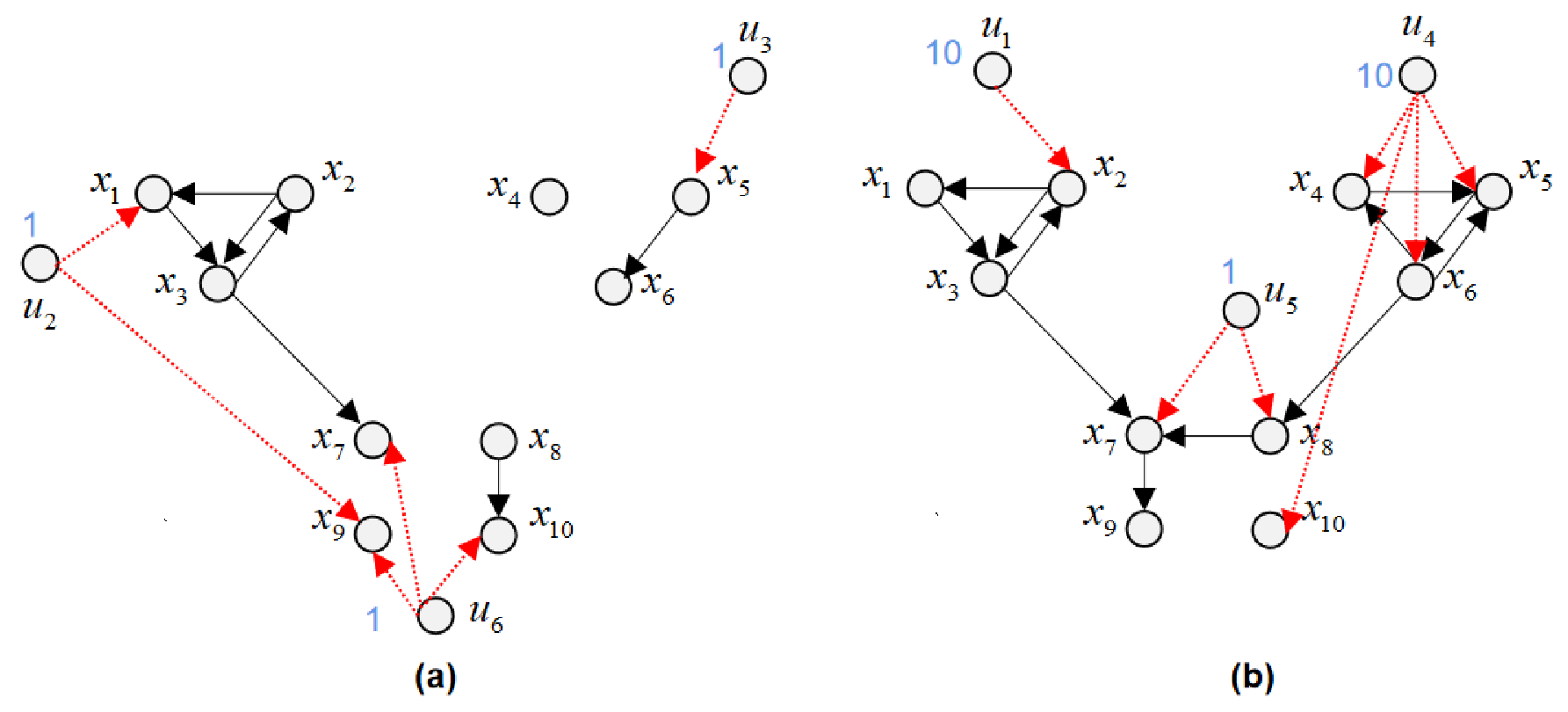
We provide two examples here to illustrate the effectiveness of the proposed methods.
Example 3
Consider system with its system digraph given in Fig. 4, which has inputs, states, and edges. The cost of inputs is . This system contains two source-SCCs, with and . Hence, . As no inputs connect with and simultaneously, the SSSI constraint is met. The corresponding matrix
Construct LPs and with decision variables , and .
Using the Matlab LP solver linprog to solve the LP associated with this system, we obtain , implying the optimum . This means the optimal solution is , and the corresponding minimum cost is . Remarkably, this result is consistent with the one obtained via the LP-rounding.
Next, we solve the LP with to obtain the integral optimal solution (see footnote 2 on how to obtain the integral solution from a fractional one). And we obtain , with the optimum . This means the optimal solution with a cardinality upper bound is , and the corresponding cost is . Finally, we set and then reduces to determining the minimum number of inputs to achieve structural controllability. We obtain for and otherwise. Hence, the minimum number of inputs for structural controllability is , with the optimal solution . If we consider the original input cost , this solution has cost , which can also be obtained by setting in .
Example 4
Consider a switched system with two switching modes. The system digraphs of subsystems and are given in Figs. 5(a) and (b), which implies . Let the cost of inputs be (i.e., the same as in Example 3). On the one hand, for subsystem , connects with the source-SCCs and , while for subsystem , connects with the source-SCCs and simultaneously. This indicates each subsystem does not satisfy the SSSI constraint. On the other hand, it is easy to check that the system digraph of the corresponding is exactly Fig. 4. Therefore, the whole system satisfies the joint SSSI constraint. By Theorem 4, we could adopt the LP-relaxations to solve and associated with this system.
To this end, let us build with . Solving yields with the corresponding cost . Hence, this minimum cost switched input selection with no more than inputs is that, selecting for subsystem and for subsystem . If we set , then solving returns the solution , with the cost . This implies, selecting for subsystem and for subsystem incurs the minimum cost with no more than inputs.
Comparing Examples 3 and 4, we find: 1) both for a fixed (non-switched) and a switched system, with a bigger cardinality upper bound, the cost of the obtained solution tends to be smaller. This highlights the significance of the cardinality-constrained minimum cost input selections and ; 2) even though the ‘union’ of subsystems (i.e., ) of the switched system is the same as the fixed system, the former tends to have smaller input costs for achieving structural controllability under the same cardinality constraint. This is consistent with the fact that switched systems are often more efficient (in terms of the number of inputs, control energy, etc.) to be controlled than the non-switched ones [35].
9 Conclusions
In this paper, we explore polynomially solvable conditions for the (cardinality-constrained) minimum cost input selection problems both for non-switched and switched structured systems. Though the NP-hardness in general, we reveal that if the input structure satisfies certain regulations, characterized by the restricted TU of the input-source-SCC incidence matrix, irrespective of the connections between each input and the states within the same source-SCC or from the non-source-SCCs, those problems are polynomially solvable via solving the corresponding LP-relaxations. A particular case is the SSSI constraint, which often emerges in some practical systems, and has been extended to the switched systems, resulting in the joint SSSI constraint. In the general case, we obtain some lower and upper bounds for the considered problems via LP-relaxation and LP-rounding. It is still unclear how to solve those problems using graph-theoretic algorithms under the addressed conditions, which could be the future work, perhaps with the help of the LP primal-dual algorithms [30].
Appendix: Proof of restricted TU
Proof of the extended SSSI constraint: Under this constraint, is a block-diagonal matrix. It suffices to show that every nonzero diagonal block of , which is a matrix with all entries being , denoted as , is restrictedly TU. Since every square submatrix of has a determinant being either (if the dimension is greater than ) or (if the dimension is ), is restrictedly TU by definition.
Proof of the row-monotone and column-monotone constraints: First, we show for any , the following matrix is restrictedly TU:
Since contains a row , it suffices to show is TU. Consider any square submatrix of . As is row-monotone and column-monotone, so is . Hence, either contains a zero column or two identical columns, or is upper triangular with all diagonal entries being . This means, , proving that is TU. Consequently, any sub-matrix of is restrictedly TU by definition. Now consider a row-monotone . If all rows of are non-decreasing, then each row must be a row of . Remove all the repeated rows from and do some row permutations on the resulted matrix, and we can obtain a matrix that is a sub-matrix of . Note as proved, is restrictedly TU. Since row (as well as column permutations) will not change the absolute value of determinants, and removing repeated rows will not affect the property of being restrictedly TU (by definition), it turns out that is restrictedly TU. The case that all rows of are non-increasing follows a similar way, and so does the case that is column-monotone.
Proof of the permutable row/column-monotone constraint: Since row and column permutations will not change the absolute value of determinants, the restricted TU follows directly from the fact that row (column)-monotone is restrictedly TU.
References
References
- [1] Y. Y. Liu, J. J. Slotine, A. L. Barabasi, Controllability of complex networks, Nature 48 (7346) (2011) 167–173.
- [2] A. Olshevsky, Minimal controllability problems, IEEE Transactions on Control of Network Systems 1 (3) (2014) 249–258.
- [3] T. H. Summers, F. L. Cortesi, J. Lygeros, On submodularity and controllability in complex dynamical networks, IEEE Transactions on Control of Network Systems 3 (1) (2016) 91–101.
- [4] F. Pasqualetti, S. Zampieri, F. Bullo, Controllability metrics, limitations and algorithms for complex networks, IEEE Transactions on Control of Network Systems 1 (1) (2014) 40–52.
- [5] H. Zhang, R. Ayoub, S. Sundaram, Sensor selection for kalman filtering of linear dynamical systems: Complexity, limitations and greedy algorithms, Automatica 78 (2017) 202–210.
- [6] S. A. Nugroho, A. F. Taha, N. Gatsis, T. H. Summers, R. Krishnan, Algorithms for joint sensor and control nodes selection in dynamic networks, Automatica 106 (2019) 124–133.
- [7] Y. Zhang, T. Zhou, Structural controllability of an NDS with LFT parameterized subsystems, IEEE Transactions on Automatic Control 64 (12) (2019) 4920–4935.
- [8] T. Ikeda, K. Kashima, Sparsity-constrained controllability maximization with application to time-varying control node selection, IEEE Control Systems Letters 2 (3) (2018) 321–326.
- [9] Y. Zhang, T. Zhou, Input matrix construction and approximation using a graphic approach, International Journal of Control 93 (7) (2020) 1577–1590.
- [10] C. Commault, J. M. Dion, Input addition and leader selection for the controllability of graph-based systems, Automatica 48 (2013) 3322–3328.
- [11] A. Olshevsky, Minimum input selection for structural controllability, in: American Control Conference, IEEE, 2015, pp. 2218–2223.
- [12] S. Pequito, S. Kar, A. P. Aguiar, Minimum cost input/output design for large-scale linear structural systems, Automatica 68 (2016) 384–391.
- [13] Y. Zhang, Y. Xia, Y. Zhan, A linear programming approach to the minimum cost sparsest input selection for structured systems, in: 2022 American Control Conference (ACC), IEEE, 2022, pp. 1453–1458.
- [14] Y. Zhang, T. Zhou, Minimal structural perturbations for controllability of a networked system: Complexities and approximations, International Journal of Robust and Nonlinear Control 29 (12) (2019) 4191–4208.
- [15] S. Pequito, S. Kar, A. P. Aguiar, On the complexity of the constrained input selection problem for structural linear systems, Automatica 62 (2015) 193–199.
- [16] S. Moothedath, P. Chaporkar, M. N. Belur, A flow-network-based polynomial-time approximation algorithm for the minimum constrained input structural controllability problem, IEEE Transactions on Automatic Control 63 (9) (2018) 3151–3158.
- [17] Y. Zhang, On constrained input selections for structured systems: Polynomially solvable cases, in: IEEE Conference on Decision and Control, IEEE, 2022, to appear.
- [18] J. M. Dion, C. Commault, J. Van DerWoude, Generic properties and control of linear structured systems: a survey, Automatica 39 (2003) 1125–1144.
- [19] C. T. Lin, Structural controllability, IEEE Transactions on Automatic Control 19 (3) (1974) 201–208.
- [20] Z. Sun, S. S. Ge, T. H. Lee, Controllability and reachability criteria for switched linear systems, Automatica 48 (5) (2002) 775–786.
- [21] X. Liu, H. Lin, B. M. Chen, Structural controllability of switched linear systems, Automatica 49 (12) (2013) 3531–3537.
- [22] S. Pequito, G. J. Pappas, Structural minimum controllability problem for switched linear continuous-time systems, Automatica 78 (2017) 216–222.
- [23] A. Schrijver, Theory of Linear and Integer Programming, John Wiley & Sons, 1998.
- [24] P. M. Vaidya, Speeding-up linear programming using fast matrix multiplication, in: 30th Annual Symposium on Foundations of Computer Science, IEEE, 1989, pp. 332–337.
- [25] G. Labahn, V. Neiger, W. Zhou, Fast, deterministic computation of the hermite normal form and determinant of a polynomial matrix, Journal of Complexity 42 (2017) 44–71.
- [26] J. Poggiale, From behavioural to population level: growth and competition, Mathematical and Computer Modelling 27 (4) (1998) 41–49.
- [27] C. H. G. Ferreira, F. M. Ferreira, B. de Sousa Matos, J. M. de Almeida, Modeling dynamic ideological behavior in political networks, The Journal of Web Science 7 (2019) 1–14.
- [28] A.-L. Barabási, R. Albert, Emergence of scaling in random networks, science 286 (5439) (1999) 509–512.
- [29] S. Assadi, S. Khanna, Y. Li, V. M. Preciado, Complexity of the minimum input selection problem for structural controllability, IFAC-PapersOnLine 48 (22) (2015) 70–75.
- [30] E. L. Lawler, Combinatorial Optimization: Networks and Matroids, Courier Corporation, 2001.
- [31] A. J. Hoffman, J. B. Kruskal, Integral boundary points of convex polyhedra, in: Linear Inequalities and Related Systems.(AM-38), Vol. 38,Chapter 13, Princeton University Press, 1956.
- [32] S. Boyd, S. P. Boyd, L. Vandenberghe, Convex Optimization, Cambridge university press, 2004.
- [33] K. Murota, Matrices and Matroids for Systems Analysis, Springer Science Business Media, 2009.
- [34] B. Hou, X. Li, G. Chen, Structural controllability of temporally switching networks, IEEE Transactions on Circuits and Systems I: Regular Papers 63 (10) (2016) 1771–1781.
- [35] A. Li, S. P. Cornelius, Y.-Y. Liu, L. Wang, A.-L. Barabási, The fundamental advantages of temporal networks, Science 358 (6366) (2017) 1042–1046.